The need for the Higgs boson in the Standard Model

Abstract

We review the role of the Higgs boson in preserving unitarity of the scattering amplitudes in the Standard Model (SM). We will look at the processes $\nu_{e}+\overline{\nu}_{e}\rightarrow W^{-}_{L}+W^{+}_{L}$, $W^{-}_{L}+W^{+}_{L}\rightarrow W^{-}_{L}+W^{+}_{L}$ and $e^{-}+e^{+}\rightarrow W^{-}_{L}+W^{+}_{L}$ for longitudinally polarized gauge bosons. Special emphasis will be put in using algebraic methods to evaluate the amplitudes and cross sections. This note is based on Lectures given at the IDPASC Schools at Udine (2012) and Braga (2014).

I Introduction

As we will be talking about cancellations, the conventions for the vertices of the SM are very important. So we will collect here all the necessary couplings for our purposes. We will also discuss the polarization vectors of the gauge bosons, particularly the longitudinal polarization vector and the implications of unitarity on the growth of the amplitudes with $\sqrt{s}$.

I.1 Gauge Boson Self-Couplings

\psfrag{p}{$p$}\psfrag{q}{$q$}\psfrag{k}{$k$}\psfrag{W1}{$W_{\alpha}^{-}$}\psfrag{W2}{$W_{\beta}^{+}$}\psfrag{A}{$A_{\mu}$}\includegraphics[width=65.04034pt]{itchome2009-Fig1.eps}	$-ie\left[g_{\alpha\beta}(p-k)_{\mu}+g_{\beta\mu}(k-q)_{\alpha}+g_{\mu\alpha}(q-p)_{\beta}\right]\equiv-ie\Gamma_{\alpha\beta\mu}(p,k,q)$
\psfrag{p}{$p$}\psfrag{q}{$q$}\psfrag{k}{$k$}\psfrag{W1}{$W_{\alpha}^{-}$}\psfrag{W2}{$W_{\beta}^{+}$}\psfrag{Z}{$Z_{\mu}$}\includegraphics[width=65.04034pt]{itchome2009-Fig2.eps}	$ig\cos\theta_{W}\left[g_{\alpha\beta}(p-k)_{\mu}+g_{\beta\mu}(k-q)_{\alpha}+g_{\mu\alpha}(q-p)_{\beta}\right]\equiv ig\Gamma_{\alpha\beta\mu}(p,k,q)$
\psfrag{W1}{$W_{\alpha}^{-}$}\psfrag{W2}{$W_{\beta}^{+}$}\psfrag{W3}{$W_{\mu}^{+}$}\psfrag{W4}{$W_{\nu}^{-}$}\includegraphics[width=65.04034pt]{itchome2009-Fig3.eps}	$ig^{2}\left[2g_{\alpha\nu}g_{\beta\mu}-g_{\alpha\mu}g_{\beta\nu}-g_{\alpha\beta}g_{\mu\nu}\right]$

Figure 1: Gauge boson self-couplings

where we have defined, for future convenience,

$$\Gamma_{\alpha\beta\mu}(p,k,q)\equiv\left[g_{\alpha\beta}(p-k)_{\mu}+g_{\beta\mu}(k-q)_{\alpha}+g_{\mu\alpha}(q-p)_{\beta}\right]$$ (1)

with the convention for the momenta and charge of the particle, given in the figure.

I.2 Gauge Couplings to Fermions

\psfrag{x1}{$\psi_{d,u}$}\psfrag{x2}{$\psi_{u,d}$}\psfrag{x3}{$\psi_{f}$}\psfrag{W}{$W^{\pm}_{\mu}$}\psfrag{Z}{$Z_{\mu}$}\psfrag{A}{$A_{\mu}$}\psfrag{v1}{$\displaystyle i\frac{g}{\sqrt{2}}\gamma_{\mu}\frac{1-\gamma_{5}}{2}$}\psfrag{v2}{$\displaystyle i\frac{g}{\cos\theta_{W}}\gamma_{\mu}\left(g_{V}^{f}-g_{A}^{f}\gamma_{5}\right)$}\psfrag{v3}{$\displaystyle-ieQ_{f}\gamma_{\mu}$}\includegraphics[width=455.24408pt]{ex-itc2008-Fig2.eps}

Figure 2: Gauge couplings to fermions

where

$$g_{V}^{f}=\frac{1}{2}T_{3}^{f}-Q_{f}\sin^{2}\theta_{W},\quad g_{A}^{f}=\frac{1}{2}T_{3}^{f}$$ (2)

Sometimes it is more useful to write these couplings in terms of the left and right projectors

$$P_{L}=\frac{1-\gamma_{5}}{2},\quad P_{R}=\frac{1+\gamma_{5}}{2},\quad$$ (3)

We get

$$g_{V}^{f}-g_{A}^{f}\gamma_{5}=g_{L}^{f}P_{L}+g_{R}^{f}P_{R}$$ (4)

where

$$g_{L}^{f}=g_{V}^{f}+g_{A}^{f}=T_{3}^{f}-Q_{f}\sin^{2}\theta_{W},\qquad g_{R}^{f}=g_{V}^{f}-g_{A}^{f}=-Q_{f}\sin^{2}\theta_{W}$$ (5)

I.3 Higgs Boson Couplings

Figure 3: Higgs boson couplings

I.4 Polarization Vectors

In many problems with massive gauge bosons we do not measure their polarization, and therefore we sum over all polarizations using the well known result,

$$\sum_{\lambda}\varepsilon^{\mu}(k,\lambda)\varepsilon^{*\nu}(k,\lambda)=-g^{\mu\nu}+\frac{k^{\mu}k^{\nu}}{M_{W}^{2}}$$ (6)

where we used the $W$ boson as an example. As we will be considering the case of longitudinal polarized gauge bosons, we have to review the expressions for the polarization vectors. Let us start with the case of longitudinal polarization. In the gauge boson rest frame (we consider here the case of the $W$, but similar expressions apply also for the case of the $Z$) where $p^{\mu}=(M_{W},0,0,0)$, the longitudinal polarization vector is

$$\varepsilon^{\mu}_{L}(p)=(0,0,0,1),\quad\hbox{satisfying}\quad\varepsilon_{L}(p)\cdot\varepsilon_{L}(p)=-1,\varepsilon_{L}(p)\cdot p=0\ .$$ (7)

In the frame where the gauge boson is moving with velocity $\vec{\beta}$ we have

$$\varepsilon^{\mu}_{L}(p)=(\gamma\beta,\gamma\hat{\beta})$$ (8)

where, as usually, $\vec{\beta}=\vec{p}/E$, $\gamma^{-1}=\sqrt{1-\beta^{2}}$ e $\hat{\beta}=\vec{\beta}/\beta$, verifying the invariant relations $\varepsilon_{L}(p)\cdot\varepsilon_{L}(p)=-1$ e $\varepsilon_{L}(p)\cdot p=0$. For $E\gg M_{W}$ we also have approximately

$$\varepsilon^{\mu}_{L}(p)\simeq\frac{p^{\mu}}{M_{W}}$$ (9)

We should notice that this relation is only approximate and can not be applied in all cases (the invariant relations are violated by terms of the order of $M_{W}^{2}/E^{2}$). In fact, one can easily show that a better approximation is

$$\varepsilon^{\mu}_{L}(p)=\frac{p^{\mu}}{M_{W}}+\frac{1}{2\gamma^{2}}\frac{Q^{\mu}}{M_{W}}+\cdots$$ (10)

where

$$Q^{\mu}=\left(-E,\vec{p}\right)$$ (11)

With this relation one can show that

$$\varepsilon_{L}(p)\cdot\varepsilon_{L}(p)=-1+\mathcal{O}\left(\frac{1}{\gamma^{4}}\right),\quad\varepsilon_{L}(p)\cdot p=0+\mathcal{O}\left(\frac{1}{\gamma^{4}}\right)$$ (12)

We will see below that, depending on the case, one can use the simpler Eq. (9), the more correct Eq. (10) or the exact expression in Eq. (8).

Now we consider the case of transverse polarized gauge bosons. Here we have in the frame where the gauge boson moves along the $z$ axis, that is, $p^{\mu}=E_{W}(1,0,0,\beta)$ that the two degrees of transverse polarization can be written as

$$\varepsilon^{\mu}_{T}=(0,\vec{\varepsilon}_{T_{1,2}})$$ (13)

where $\vec{\varepsilon}_{T_{1,2}}$ lie in the plane perpendicular to the $z$ axis. Any combination of linearly independent vectors will do, but there are obviously two preferred choices. The first one, corresponds to two linearly polarized perpendicular vectors,

$$\varepsilon^{\mu}_{T_{1}}=(0,1,0,0),\quad\varepsilon_{T_{1}}=(0,0,1,0)$$ (14)

and the other choice corresponds to helicity $\pm$,

$$\varepsilon^{\mu}_{\pm}=(0,\frac{1}{\sqrt{2}},\pm\frac{i}{\sqrt{2}},0)$$ (15)

satisfying the correct normalization conditions $\varepsilon(p)\cdot\varepsilon^{*}(p)=-1,\varepsilon(p)\cdot p=0$. Note that for the case of helicity vectors, as they are complex, we have to take the complex conjugate in the normalization condition. In real situations the gauge bosons will be moving along some direction $\vec{\beta}=\vec{k}/E_{W}$ with respect to some reference frame, usually defined by the incident particles. If we have the situation indicated in Fig. 4

\psfrag{x}{$x$}\psfrag{xp}{$x^{\prime}$}\psfrag{z}{$z$}\psfrag{zp}{$z^{\prime}$}\psfrag{t}{$\theta$}\psfrag{y}{$y=y^{\prime}$}\psfrag{k}{$\vec{k}$}\includegraphics[width=156.49014pt]{kingaugeboson.eps}

Figure 4: Kinematics of the gauge boson

then we will have for the two choices of polarization vectors,

$$\varepsilon^{\mu}(\lambda=\pm)=(0,\frac{1}{\sqrt{2}}\cos\theta,\pm\frac{i}{\sqrt{2}},-\frac{1}{\sqrt{2}}\sin\theta)$$ (16)

and

$$\varepsilon^{\mu}(\lambda=\vec{e}_{x})=(0,\cos\theta,0,-\sin\theta),\quad\varepsilon^{\mu}(\lambda=\vec{e}_{y})=(0,0,1,0)$$ (17)

We leave it for the reader to verify that using the definitions of Eqs. (8) and (16) or (17) we can reproduce the general result of the sum over all polarizations, Eq. (6). Also a more compact expression for the polarization vector, valid for all polarizations, can be shown to be given by quigg:1983 ,

$$\varepsilon^{\mu}=\left[\gamma(\vec{\beta}\cdot\vec{\varepsilon}),\vec{\varepsilon}+(\gamma-1)(\hat{\beta}\cdot\vec{\varepsilon})\hat{\beta}\right]$$ (18)

where $\vec{\varepsilon}$ is the polarization vector in the rest frame of the gauge boson.

I.5 Unitarity and Growth of the Amplitudes with $\sqrt{s}$

The last topic we want to discuss in this introduction is the behavior of the amplitudes with the growth of the center of mass energy. For these $1+2\rightarrow 3+4$ processes, it can be shown quigg:1983 , that the amplitudes for large values of $\sqrt{s}$ should, at most, be constant with the energy,

$$\lim_{\sqrt{s}\rightarrow\infty}\mathcal{M}=\hbox{constant.}$$ (19)

This in turn will imply that the cross sections given by romao:2016itc ,

$$\frac{d\sigma}{d\Omega}=\frac{1}{64\pi^{2}\,s}\ \frac{|\vec{p}_{\rm 3CM}|}{|\vec{p}_{\rm 1CM}|}\ \overline{|\mathcal{M}|}^{2}$$ (20)

will decrease for values of $\sqrt{s}\gg M$, where $M$ is any mass in the problem.

II The scattering $\nu_{e}+\overline{\nu}_{e}\rightarrow W^{+}_{L}+W^{-}_{L}$

As a first exercise on the structure of the SM we will look at the process

$$\nu_{e}(p_{1})+\overline{\nu}_{e}(p_{2})\rightarrow W^{+}_{L}(q_{1})+W^{-}_{L}(q_{2})$$ (21)

In the SM this process has the tree-level diagrams shown in Fig. 5.

\psfrag{n}{$\nu_{e}$}\psfrag{nb}{$\overline{\nu}_{e}$}\psfrag{Wp}{$W^{+}$}\psfrag{Wm}{$W^{-}$}\psfrag{e}{$e$}\psfrag{g}{$\gamma$}\psfrag{Z}{$Z$}\includegraphics{nuNuWLWL.eps}

Figure 5: Diagrams contributing to $\nu_{e}+\overline{\nu}_{e}\rightarrow W^{+}_{L}+W^{-}_{L}$.

The kinematics in the CM frame is given in Fig. 6, where $\theta_{\rm CM}$ is the scattering angle in the CM frame.

\psfrag{t}{$\theta_{\rm CM}$}\psfrag{p1}{$p_{1}$}\psfrag{p2}{$p_{2}$}\psfrag{q1}{$q_{1}$}\psfrag{q2}{$q_{2}$}\includegraphics{CMkinematics.eps}

Figure 6: CM kinematics.

which can be written as

$$\left\{\begin{array}[]{l}\displaystyle p_{1}=\frac{\sqrt{s}}{2}(1,0,0,1)\\[5.69054pt] \displaystyle p_{2}=\frac{\sqrt{s}}{2}(1,0,0,-1)\\[5.69054pt] \displaystyle q_{1}=\frac{\sqrt{s}}{2}(1,\beta\sin\theta_{\rm CM},0,\beta\cos\theta_{\rm CM})\\[5.69054pt] \displaystyle q_{2}=\frac{\sqrt{s}}{2}(1,-\beta\sin\theta_{\rm CM},0,-\beta\cos\theta_{\rm CM})\\[5.69054pt] \end{array}\right.$$ (22)

where $\beta$ is the velocity of the $W$ in the CM frame,

$$\beta=\sqrt{1-\frac{4M_{W}^{2}}{s}}$$ (23)

It is also important to write down the explicit expressions for the longitudinal polarization vectors. We have

$$\begin{array}[]{l}\displaystyle\varepsilon_{L}^{\mu}(q_{1})=\frac{\sqrt{s}}{2M_{W}}(\beta,\sin\theta_{\rm CM},0,\cos\theta_{\rm CM})\\[8.53581pt] \displaystyle\varepsilon_{L}^{\mu}(q_{2})=\frac{\sqrt{s}}{2M_{W}}(\beta,-\sin\theta_{\rm CM},0,-\cos\theta_{\rm CM})\\[8.53581pt] \end{array}$$ (24)

II.1 The Amplitudes

Let us begin by writing the amplitudes for the two diagrams. We have (in this case it is safe to neglect the electron mass in the propagator)

$$\mathcal{M}_{t}= -\frac{g^{2}}{2}\overline{v}(p_{2})\gamma_{\nu}(/{p}_{1}-/{q}_{1})\gamma_{\mu}u(p_{1})\frac{1}{t}\ \varepsilon^{\mu}_{L}(q_{1})\varepsilon^{\nu}_{L}(q_{2})$$

$$\mathcal{M}_{s}= -\frac{g^{2}}{2}\overline{v}(p_{2})\gamma_{\alpha}P_{L}u(p_{1})\left[-g^{\alpha\beta}+\frac{(p_{1}+p_{2})^{\alpha}(p_{1}+p_{2})^{\beta}}{M_{W}^{2}/c_{W}^{2}}\right]\frac{\Gamma_{\mu\nu\beta}(-q_{1},-q_{2},q_{1}+q_{2})}{s-M_{W}^{2}/c_{W}^{2}}\ \varepsilon^{\mu}_{L}(q_{1})\varepsilon^{\nu}_{L}(q_{2})$$

$$={} \frac{g^{2}}{2}\overline{v}(p_{2})\gamma^{\alpha}P_{L}u(p_{1})\frac{\Gamma_{\mu\nu\alpha}(-q_{1},-q_{2},q_{1}+q_{2})}{s-M_{W}^{2}/c_{W}^{2}}\ \varepsilon^{\mu}_{L}(q_{1})\varepsilon^{\nu}_{L}(q_{2})$$ (25)

where we have used the SM relation $M_{W}=M_{Z}c_{W}$ with $c_{W}=\cos\theta_{W}$ and, in the last step, we have used the Dirac equation and the fact that the neutrinos (in the SM) have no mass to simplify the numerator of the $Z$ propagator.

II.2 Unitarity and the cancellation of the bad behavior

We can convince ourselves easily that each of the amplitudes in Eq. (II.1) do not obey the constraint from unitarity, Eq. (19). To see that one has to understand that at high energy we have

$$\overline{v}(p_{2})u(p_{1})\propto\sqrt{s},\quad p_{i},q_{i}\propto\sqrt{s},\quad\varepsilon^{\mu}_{L}(q_{i})\propto\frac{\sqrt{s}}{M_{W}}$$ (26)

and therefore

$$\mathcal{M}_{t},\mathcal{M}_{s}\propto s$$ (27)

Then, unless there is a cancellation between the fastest growing terms with $\sqrt{s}$, we will have a problem. This cancellation comes about because gauge invariance of the theory forces the couplings to be related. To see this let us start by the simplest formula for the longitudinal polarization, Eq. (9). Using this relation we obtain

$$\mathcal{M}_{t}=\frac{1}{2M_{W}^{2}}\overline{v}(p_{2})/{q}_{2}P_{L}u(p_{1})+\mathcal{O}\left(1\right)\ .$$ (28)

which indeed shows that the amplitude grows with $s$. If we do the same for the s-channel diagram of the $Z$, we obtain,

$$\mathcal{M}_{s}={} \frac{1}{4M_{W}^{2}}\overline{v}(p_{2})/{q}_{1}P_{L}u(p_{1})-\frac{1}{4M_{W}^{2}}\overline{v}(p_{2})/{q}_{2}P_{L}u(p_{1})+\mathcal{O}\left(1\right)$$

$$= -\frac{1}{2M_{W}^{2}}\overline{v}(p_{2})/{q}_{2}P_{L}u(p_{1})+\mathcal{O}\left(1\right)$$ (29)

where we have used $q_{1}=-q_{2}+p_{1}+p_{2}$ and the Dirac equation for massless neutrinos. We therefore obtain,

$$\mathcal{M}=\mathcal{M}_{\nu}+\mathcal{M}_{Z}=\mathcal{O}\left(1\right)$$ (30)

in agreement with Eq. (19). It should be stressed that the cancellation depends on the relation between the couplings of different particles and these were dictated by gauge invariance.

II.3 Cross section

Let us calculate the cross section to display the effect of the cancellation. Writing, in an obvious notation,

$$|\mathcal{M}|^{2}=|\mathcal{M}_{t}|^{2}+|\mathcal{M}_{s}|^{2}+\left(\mathcal{M}_{t}\mathcal{M}_{s}^{*}+\mathcal{M}_{t}^{*}\mathcal{M}_{s}\right)$$ (31)

we get (see Appendix A.1 for an input file for the Mathematica package FeynCalc),

$$|\mathcal{M}_{t}|^{2}= -\frac{g^{4}\left(4M_{W}^{4}+st\right)^{2}\left[M_{W}^{4}-2M_{W}^{2}t+t(s+t)\right]}{4M_{W}^{4}t^{2}\left(s-4M_{W}^{2}\right)^{2}}$$

$$={} g^{4}\left[\sin^{2}\theta\ x^{2}+\sin^{2}\theta\ x-\cos^{2}\theta-\cos\theta+\mathcal{O}\left(x^{-1}\right)\right]$$ (32)

where we have defined $\displaystyle x=\frac{s}{4M_{W}^{2}}$ and the expansion is for $x\gg 1$. Similarly for the s-channel $Z$ exchange we get,

$$|\mathcal{M}_{s}|^{2}= -\frac{g^{4}\left(2M_{W}^{2}+s\right)^{2}\left(M_{W}^{4}-2M_{W}^{2}t+t(s+t)\right)}{4M_{W}^{4}\left(M_{Z}^{2}-s\right)^{2}}$$

$$={} g^{4}\left[\sin^{2}\theta\ x^{2}+\frac{M_{Z}^{2}\sin^{2}\theta}{2M_{W}^{2}}\ x+\frac{3M_{Z}^{4}\sin^{2}\theta}{16M_{W}^{4}}-\frac{3\sin^{2}\theta}{4}+\mathcal{O}\left(x^{-1}\right)\right]$$ (33)

and for the interference term

$$\left(\mathcal{M}_{t}\mathcal{M}_{s}^{*}+\mathcal{M}_{t}^{*}\mathcal{M}_{s}\right)={} \frac{g^{4}\left(8M_{W}^{10}+4M_{W}^{8}(s-4t)+2M_{W}^{6}t(s+4t)+5M_{W}^{4}s^{2}t+2M_{W}^{2}st^{3}+s^{2}t^{2}(s+t)\right)}{2M_{W}^{4}t\left(4M_{W}^{2}-s\right)\left(M_{Z}^{2}-s\right)}$$ (34)

$$={} g^{4}\left[-2\sin^{2}\theta\ x^{2}-\sin^{2}\theta\ x-\frac{M_{Z}^{2}\sin^{2}\theta}{2M_{W}^{2}}\ x+\cos\theta+1-\frac{M_{Z}^{4}\sin^{2}\theta}{8M_{W}^{4}}-\frac{M_{Z}^{2}\sin^{2}\theta}{4M_{W}^{2}}+\mathcal{O}\left(x^{-1}\right)\right]$$

One can see by looking at Eqs. (II.3), (II.3) and (34) that the terms proportional to $x^{2}$ and $x$ exactly cancel and that, at high energy the behavior is

$$|\mathcal{M}|^{2}=\frac{g^{4}\sin^{2}\theta\left(M_{Z}^{2}-2M_{W}^{2}\right)^{2}}{16M_{W}^{4}}+\mathcal{O}\left(x^{-1}\right)$$ (35)

consistent with Eq. (19). The behavior of the various terms is shown in Fig. 7.

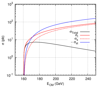
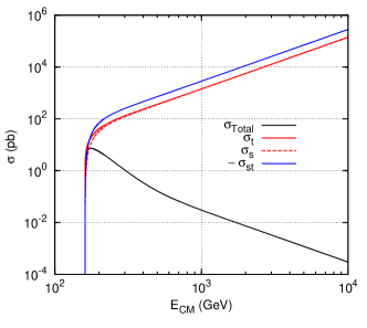
Figure 7: Cross section for the process $\nu_{e}+\overline{\nu}_{e}\rightarrow W^{+}_{L}+W^{-}_{L}$. Displayed are the total cross section (black), as well as the s-channel (red-dashed), t-channel (red) and the interference (blue). As the interference is negative we plot its absolute value. On the left panel the range of $\sqrt{s}$ is smaller to show the details at threshold. On the right panel the behavior at high energy $\sqrt{s}\gg M_{W}$, is already present. Notice the log scale on $\sqrt{s}$ on the right panel.

We leave as an exercise to the reader to check that introducing Eq. (35) in Eq. (20) one can reproduce the high energy behavior of the right panel of Fig. 7 with a relative error below $10^{-2}$ already for $\sqrt{s}=260$ GeV and below $10^{-4}$ for $\sqrt{s}=500$ GeV.

III The scattering of longitudinal gauge bosons: $W^{-}_{L}(p_{1})+W^{+}_{L}(p_{2})\rightarrow W^{-}_{L}(q_{1})+W^{+}_{L}(q_{2})$

The next process that we will consider is the scattering of longitudinal $W^{\pm}_{L}$.

$$W^{-}_{L}(p_{1})+W^{+}_{L}(p_{2})\rightarrow W^{-}_{L}(q_{1})+W^{+}_{L}(q_{2})$$ (36)

where the momenta are as indicated and the subscript $L$ means that the gauge bosons $W^{\pm}$ are longitudinally polarized. In the SM this process has seven tree-level diagrams shown in Fig. 8.

\psfrag{h}{$h$}\psfrag{Wm}{$W^{-}$}\psfrag{Wp}{$W^{+}$}\psfrag{gZ}{$\gamma,Z$}\includegraphics[width=433.62pt]{WLWLWLWL.eps}

Figure 8: Diagrams contributing to $W^{-}_{L}+W^{+}_{L}\rightarrow W^{-}_{L}+W^{+}_{L}$.

with the kinematics,

$$\left\{\begin{array}[]{l}\displaystyle p_{1}=\frac{\sqrt{s}}{2}(1,0,0,\beta)\\[5.69054pt] \displaystyle p_{2}=\frac{\sqrt{s}}{2}(1,0,0,-\beta)\\[5.69054pt] \displaystyle q_{1}=\frac{\sqrt{s}}{2}(1,\beta\sin\theta_{\rm CM},0,\beta\cos\theta_{\rm CM})\\[5.69054pt] \displaystyle q_{2}=\frac{\sqrt{s}}{2}(1,-\beta\sin\theta_{\rm CM},0,-\beta\cos\theta_{\rm CM})\\[5.69054pt] \end{array}\right.\qquad\left\{\begin{array}[]{l}\displaystyle\varepsilon_{L}(p_{1})=\frac{\sqrt{s}}{2M_{W}}(\beta,0,0,1)\\[5.69054pt] \displaystyle\varepsilon_{L}(p_{2})=\frac{\sqrt{s}}{2M_{W}}(\beta,0,0,-1)\\[5.69054pt] \displaystyle\varepsilon_{L}(q_{1})=\frac{\sqrt{s}}{2M_{W}}(\beta,\sin\theta_{\rm CM},0,\cos\theta_{\rm CM})\\[5.69054pt] \displaystyle\varepsilon_{L}(q_{2})=\frac{\sqrt{s}}{2M_{W}}(\beta,-\sin\theta_{\rm CM},0,-\cos\theta_{\rm CM})\\[5.69054pt] \end{array}\right.$$ (37)

where, as before, $\beta=\sqrt{1-4M_{W}^{2}/s}$. Notice that the invariant relations of the type $\varepsilon_{L}(p_{1})\cdot\varepsilon_{L}(p_{1})=-1$ and $\varepsilon_{L}(p_{1})\cdot p_{1}=0$ are verified for all cases. We will see that this case is very interesting, because not only the gauge structure is necessary for the amplitudes to have the correct behavior, as in the previous case, but also the Higgs boson is fundamental.

III.1 The Amplitudes

Let us denote, in an obvious notation, the amplitudes as

$$\mathcal{M}=\mathcal{M}_{\gamma+Z}^{s}+\mathcal{M}_{\gamma+Z}^{t}+\mathcal{M}_{4W}+\mathcal{M}_{H}^{s+t}$$ (38)

We have then,

$$\mathcal{M}_{\gamma}^{s}={} \frac{g^{2}s_{W}^{2}}{s}\ \epsilon_{L}^{\alpha}(p_{1})\epsilon_{L}^{\beta}(p_{2})\epsilon_{L}^{\gamma}(q_{1})\epsilon_{L}^{\delta}(q_{2})\ \Gamma_{\alpha,\beta,\mu}(p_{1},p_{2},-p_{1}-p_{2})\Gamma_{\delta,\gamma,\nu}(-q_{2},-q_{1},p_{1}+p_{2})\ g^{\mu\nu}$$

$$\mathcal{M}_{Z}^{s}={} \frac{g^{2}c_{W}^{2}}{s-M_{W}^{2}/c_{W}^{2}}\ \epsilon_{L}^{\alpha}(p_{1})\epsilon_{L}^{\beta}(p_{2})\epsilon_{L}^{\gamma}(q_{1})\epsilon_{L}^{\delta}(q_{2})\ \Gamma_{\alpha,\beta,\mu}(p_{1},p_{2},-p_{1}-p_{2})\Gamma_{\delta,\gamma,\nu}(-q_{2},-q_{1},p_{1}+p_{2})$$

$$\hskip 2.84526pt\times\left[g^{\mu\nu}-\frac{(p_{1}+p_{2})^{\mu}(p_{1}+p_{2})^{\nu}}{M_{W}^{2}/c_{W}^{2}}\right]$$

$$\mathcal{M}_{\gamma}^{t}={} \frac{g^{2}s_{W}^{2}}{t}\ \epsilon_{L}^{\alpha}(p_{1})\epsilon_{L}^{\beta}(p_{2})\epsilon_{L}^{\gamma}(q_{1})\epsilon_{L}^{\delta}(q_{2})\ \Gamma_{\alpha,\gamma,\mu}(p_{1},-q_{1},q_{1}-p_{1})\Gamma_{\delta,\beta,\nu}(-q_{2},p_{2},q_{2}-p_{2})\ g^{\mu\nu}$$

$$\mathcal{M}_{Z}^{t}={} \frac{g^{2}c_{W}^{2}}{t-M_{W}^{2}/c_{W}^{2}}\ \epsilon_{L}^{\alpha}(p_{1})\epsilon_{L}^{\beta}(p_{2})\epsilon_{L}^{\gamma}(q_{1})\epsilon_{L}^{\delta}(q_{2})\ \Gamma_{\alpha,\gamma,\mu}(p_{1},-q_{1},q_{1}-p_{1})\Gamma_{\delta,\beta,\nu}(-q_{2},p_{2},q_{2}-p_{2})$$

$$\hskip 2.84526pt\times\left[g^{\mu\nu}-\frac{(p_{1}-q_{1})^{\mu}(p_{1}-q_{1})^{\nu}}{M_{W}^{2}/c_{W}^{2}}\right]$$ (39)

$$\mathcal{M}_{4W}={} g^{2}\ \epsilon_{L}^{\alpha}(p_{1})\epsilon_{L}^{\beta}(p_{2})\epsilon_{L}^{\gamma}(q_{1})\epsilon_{L}^{\delta}(q_{2})\ \left[2g_{\alpha\delta}\,g_{\beta\gamma}-g_{\alpha\beta}\,g_{\delta\gamma}-g_{\alpha\gamma}\,g_{\delta\beta}\right]$$

$$\mathcal{M}_{H}^{s}={} -\frac{g^{2}M_{W}^{2}}{s-M_{H}^{2}}\ \epsilon_{L}^{\alpha}(p_{1})\epsilon_{L}^{\beta}(p_{2})\epsilon_{L}^{\gamma}(q_{1})\epsilon_{L}^{\delta}(q_{2})\ g_{\alpha\beta}\,g_{\gamma\delta}$$

$$\mathcal{M}_{H}^{t}={} -\frac{g^{2}M_{W}^{2}}{t-M_{H}^{2}}\ \epsilon_{L}^{\alpha}(p_{1})\epsilon_{L}^{\beta}(p_{2})\epsilon_{L}^{\gamma}(q_{1})\epsilon_{L}^{\delta}(q_{2})\ g_{\alpha\gamma}\,g_{\beta\delta}$$

where we have introduced the shorthand notation $s_{W}^{2}=\sin^{2}\theta_{W}$, $c_{W}^{2}=\cos^{2}\theta_{W}$, and made use of the SM relations $M_{W}=c_{W}M_{Z}$ and $e=gs_{W}$. If we insert the high energy behavior of $\epsilon_{L}$, Eq. (9), we see that the amplitudes can grow potentially as $s^{2}$ or even $s^{3}$ in the case of the diagrams where there is a $Z$ exchange. Therefore it is clear that the approximation of Eq. (9) is not enough. So, we start by calculating the amplitudes with no approximation, making use of Eq. (8) and of the CM kinematics of Fig. 6. We get,

$$\mathcal{M}_{\gamma}^{s}= \frac{g^{2}s_{W}^{2}}{4M_{W}^{4}s}\left(2M_{W}^{2}+s\right)^{2}\left(4M_{W}^{2}-s-2t\right)$$

$$\mathcal{M}_{Z}^{s}= \frac{g^{2}\,c_{W}^{2}}{4M_{W}^{4}\left(s-M_{W}^{2}/c_{W}^{2}\right)}\left(2M_{W}^{2}+s\right)^{2}\left(4M_{W}^{2}-s-2t\right)$$

$$\mathcal{M}_{\gamma}^{t}= \frac{g^{2}s_{W}^{2}}{4M_{W}^{4}t\left(s-4M_{W}^{2}\right)^{2}}\left[\vbox to12.0pt{}256M_{W}^{10}-64M_{W}^{8}(4s+t)+16M_{W}^{6}s(5s+14t)-4M_{W}^{4}s\left(2s^{2}+21st+20t^{2}\right)\right.$$

$$\hskip 85.35826pt\left.\vbox to12.0pt{}+8M_{W}^{2}s^{2}t(s+3t)-s^{2}t^{2}(2s+t)\right]$$

$$\mathcal{M}_{Z}^{t}= \frac{g^{2}c_{W}^{2}}{4M_{W}^{4}\left(s-4M_{W}^{2}\right)^{2}\left(t-M_{W}^{2}/c_{W}^{2}\right)}\left[\vbox to12.0pt{}256M_{W}^{10}-64M_{W}^{8}(4s+t)+16M_{W}^{6}s(5s+14t)-4M_{W}^{4}s\left(2s^{2}+21st+20t^{2}\right)\right.$$

$$\hskip 142.26378pt\left.\vbox to12.0pt{}+8M_{W}^{2}s^{2}t(s+3t)-s^{2}t^{2}(2s+t)\right]$$ (40)

$$\mathcal{M}_{4W}= \frac{g^{2}s}{4M_{W}^{4}\left(s-4M_{W}^{2}\right)^{2}}\left[\vbox to12.0pt{}-64M_{W}^{6}+48M_{W}^{4}(s+t)-4M_{W}^{2}s(3s+7t)+s\left(s^{2}+4st+t^{2}\right)\right]$$

$$\mathcal{M}_{H}^{s}= -g^{2}\frac{\left(s-2M_{W}^{2}\right)^{2}}{4M_{W}^{2}\left(s-M_{H}^{2}\right)}$$

$$\mathcal{M}_{H}^{t}= -g^{2}\,\frac{\left(-8M_{W}^{4}+2M_{W}^{2}s+st\right)^{2}}{4\left(t-M_{H}^{2}\right)\left(M_{W}s-4M_{W}^{3}\right)^{2}}$$

III.2 Unitarity and the cancellation of the bad behavior

By inspection, we see that for $\sqrt{s}\gg M_{W}$ the first five amplitudes grow as $s^{2}$ and the last two (from the Higgs exchange) as $s$. So if we define, as before, the dimensionless variable $x=s/(4M_{W}^{2})$, for $x\gg 1$ we should be able to write all amplitudes in the form

$$\mathcal{M}_{i}=A_{i}x^{2}+B_{i}x+C_{i}+\mathcal{O}(1/x)\ .$$ (41)

The results for these coefficients are summarized in Table 1.

	$A_{i}$	$B_{i}$	$C_{i}$
$\mathcal{M}_{\gamma}^{s}$	$-g^{2}4s_{W}^{2}\cos\theta$	$0$	$g^{2}3s_{W}^{2}\cos\theta$
$\mathcal{M}_{Z}^{s}$	$-g^{2}4c_{W}^{2}\cos\theta$	$-g^{2}\cos\theta$	$g^{2}\left[3\cos\theta\ c_{W}^{2}-\displaystyle\frac{\cos\theta}{4c_{W}^{2}}\right]$
$\mathcal{M}_{\gamma}^{t}$	$g^{2}\,s_{W}^{2}\left(\vbox to10.0pt{}-\cos^{2}\theta-2\cos\theta+3\right)$	$g^{2}\,8s_{W}^{2}\cos\theta$	$\displaystyle\frac{g^{2}s_{W}^{2}}{\cos\theta-1}\left(\vbox to10.0pt{}-2\cos^{2}\theta-\cos\theta-1\right)$
$\mathcal{M}_{Z}^{t}$	$g^{2}\,c_{W}^{2}\left(\vbox to10.0pt{}-\cos^{2}\theta-2\cos\theta+3\right)$	$g^{2}\left(8\cos\theta c_{W}^{2}-\displaystyle\frac{\cos\theta}{2}-\displaystyle\frac{3}{2}\right)$	$\displaystyle\frac{g^{2}}{\cos\theta-1}\left[\vbox to10.0pt{}-2\cos^{2}\theta c_{W}^{2}-\frac{\cos^{2}\theta}{2}-\cos\theta c_{W}^{2}-\frac{\cos\theta}{4c_{W}^{2}}\right.$
			$\left.\vbox to12.0pt{}+3\cos\theta-c_{W}^{2}-\frac{3}{4c_{W}^{2}}+\displaystyle\frac{3}{2}\right]$
$\mathcal{M}_{4W}$	$g^{2}\left(\vbox to10.0pt{}\cos^{2}\theta+6\cos\theta-3\right)$	$g^{2}\left(2-6\cos\theta\right)$	$0$
$\displaystyle\sum_{\gamma Z}$	$0$	$g^{2}\displaystyle\frac{1+\cos\theta}{2}$	$g^{2}3\cos\theta+\cdots$
$\mathcal{M}_{H}^{s}$	$0$	$-g^{2}$	$g^{2}\left(1-\displaystyle\frac{M_{H}^{2}}{4M_{W}^{2}}\right)$
$\mathcal{M}_{H}^{t}$	$0$	$g^{2}\left(\displaystyle\frac{1}{2}-\displaystyle\frac{\cos\theta}{2}\right)$	$-g^{2}\left[\displaystyle\frac{1+\cos\theta}{2}+\displaystyle\frac{M_{H}^{2}}{4M_{W}^{2}}\right]$
$\displaystyle\sum_{\gamma ZH}$	$0$	$0$	$\not=0$

Table 1: Coefficients $A_{i}$, $B_{i}$ and $C_{i}$ (see text for an explanation).

We see that the terms proportional to $x^{2}$ cancel among the first five diagrams involving only the gauge bosons, but that the term proportional do $x$ remains after we sum over the gauge part. So, if we consider only a gauge theory of intermediate gauge bosons, we are in trouble. This trouble can be traced back to the fact that with mass the gauge invariance is lost, and the theory is inconsistent if the diagrams involving the Higgs boson field are not taken in account. In conclusion, again the Higgs boson is crucial to make the SM consistent.

III.3 Cross section

As, in this case, the amplitudes are pure c-numbers with no spinor part, the cross section is simply obtained by summing all the amplitudes and taking the absolute value of the result to obtain $\mathcal{M}|^{2}$. The cancellation of the bad high energy behavior is shown in Fig. 9. As it is well known, there is a pole in the t-channel of the photon. To avoid that we cut in the scattering angle. Shown are the plots for two cases, $\theta_{\rm min}=1^{\circ},10^{\circ}$. The cancellation is clear in both cases.

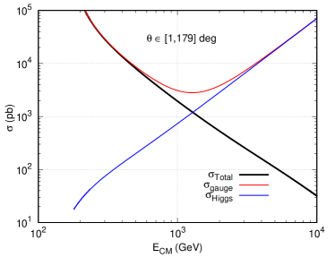
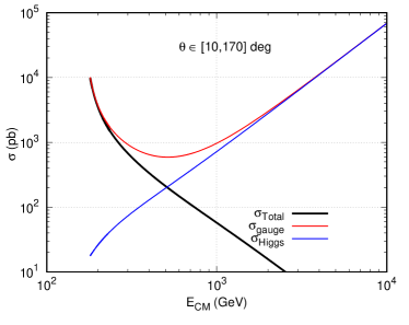
Figure 9: Cross section for $W^{-}_{L}+W^{+}_{L}\rightarrow W^{-}_{L}+W^{+}_{L}$. Shown are the contribution of the gauge diagrams (red), the contribution from the Higgs (blue) and the total cross section (black). The sum of the amplitudes from the gauge part have the opposite sign from those from the Higgs (not visible in the Fig, because we are plotting cross sections) forcing the cross section to decrease. On the left panel we consider $\theta_{\rm min}=1^{\circ}$ while in the right panel we take $\theta_{\rm min}=10^{\circ}$.

IV The scattering $e^{-}+e^{+}\rightarrow W^{-}_{L}+W^{+}_{L}$

As a last example of the importance of the Higgs boson for the consistency of the SM we consider the process,

$$e^{-}(p_{1})+e^{+}(p_{2})\rightarrow W^{-}_{L}(q_{1})+W^{+}_{L}(q_{2})$$ (42)

Compared to other two, this process has the advantage of not being an academic problem, it has in fact already been tested at the LEP experiments. In the SM this process has four tree-level diagrams shown in Fig. 10.

\psfrag{h}{$h$}\psfrag{n}{$\nu_{e}$}\psfrag{Wp}{$W^{-}$}\psfrag{Wm}{$W^{+}$}\psfrag{e}{$e^{-}$}\psfrag{p}{$e^{+}$}\psfrag{g}{$\gamma$}\psfrag{z}{$Z$}\includegraphics{eEWLWL.eps}

Figure 10: Diagrams contributing to $e^{-}+e^{+}\rightarrow W^{-}_{L}+W^{+}_{L}$.

to which correspond the the following kinematics,

$$\left\{\begin{array}[]{l}\displaystyle p_{1}=\frac{\sqrt{s}}{2}(1,0,0,\beta_{e})\\[5.69054pt] \displaystyle p_{2}=\frac{\sqrt{s}}{2}(1,0,0,-\beta_{e})\\[5.69054pt] \displaystyle q_{1}=\frac{\sqrt{s}}{2}(1,\beta\sin\theta_{\rm CM},0,\beta\cos\theta_{\rm CM})\\[5.69054pt] \displaystyle q_{2}=\frac{\sqrt{s}}{2}(1,-\beta\sin\theta_{\rm CM},0,-\beta\cos\theta_{\rm CM})\\[5.69054pt] \end{array}\right.\qquad\left\{\begin{array}[]{l}\displaystyle\varepsilon_{L}(q_{1})=\frac{\sqrt{s}}{2M_{W}}(\beta,\sin\theta_{\rm CM},0,\cos\theta_{\rm CM})\\[5.69054pt] \displaystyle\varepsilon_{L}(q_{2})=\frac{\sqrt{s}}{2M_{W}}(\beta,-\sin\theta_{\rm CM},0,-\cos\theta_{\rm CM})\\[5.69054pt] \end{array}\right.$$ (43)

where, as before, $\beta=\sqrt{1-4M_{W}^{2}/s}$ and, (we keep $m_{e}\not=0$), $\beta_{e}=\sqrt{1-4m_{e}^{2}/s}$.

IV.1 The Amplitudes

We start by writing the amplitudes for the four diagrams. As the Higgs coupling to the electrons is proportional to the electron mass, we expect, from the other examples, that for sufficiently high energy there will be a piece of the first three diagrams proportional to $m_{e}$ that will increase with energy. Therefore, we are not making any approximation with regard to $m_{e}$, and we should keep it in the calculations. We get

$$\mathcal{M}_{\nu}^{t}= -\frac{g^{2}}{2t}\overline{v}(p_{2})\gamma_{\nu}P_{L}\left(/{p}_{1}-/{q}_{1}\right)\gamma_{\mu}P_{L}u(p_{1})\ \epsilon_{L}^{\mu}(q_{1})\epsilon_{L}^{\nu}(q_{2})$$

$$\mathcal{M}_{\gamma}^{s}= -\frac{g^{2}s_{W}^{2}}{s}\overline{v}(p_{2})\gamma^{\alpha}u(p_{1})\ \Gamma_{\nu\mu\alpha}(-q_{2},-q_{1},q_{1}+q_{2})\ \epsilon_{L}^{\mu}(q_{1})\epsilon_{L}^{\nu}(q_{2})$$

$$\mathcal{M}_{Z}^{s}= -\frac{g^{2}}{s-M_{W}^{2}/c_{W}^{2}}\left[-g_{\alpha\beta}+\frac{Q^{\alpha}Q^{\beta}}{M_{W}^{2}/c_{W}^{2}}\right]\overline{v}(p_{2})\gamma^{\beta}\left(g_{L}P_{L}+g_{R}P_{R}\right)u(p_{1})\ \Gamma_{\nu\mu\alpha}(-q_{2},-q_{1},q_{1}+q_{2})\ \epsilon_{L}^{\mu}(q_{1})\epsilon_{L}^{\nu}(q_{2})$$

$$\mathcal{M}_{H}^{s}= \frac{g^{2}m_{e}}{2}\frac{1}{s-M_{H}^{2}}\ \overline{v}(p_{2})u(p_{1})\ g_{\mu\nu}\ \epsilon_{L}^{\mu}(q_{1})\epsilon_{L}^{\nu}(q_{2})$$ (44)

where we have defined $Q=p_{1}+p_{2}$, and made use again of the SM relations like $e=gs_{W}$. If we neglect for the moment $m_{e}$ this process is very much like the neutrino scattering studied in section II. Using Eq. (26) one can convince ourselves that the first three amplitudes are proportional to $s$ for $\sqrt{s}\gg m_{e},M_{W}$. However we should be careful, because the Higgs exchange diagram is proportional to $m_{e}\sqrt{s}$ and that these terms, although sub-leading, will be important for sufficiently high energy.

IV.2 Cancellation of bad high energy behavior

Let us now see how the cancellation of the bad high energy behavior is achieved in this case. One can check that it is enough to use the approximate formula of Eq. (9) to display the cancellation of the diagrams. With the help of FeynCalc we obtain

$$\mathcal{M}_{\nu}= \frac{g^{2}}{2M_{W}^{2}}\ \left[\vbox to12.0pt{}-\overline{v}(p_{2})/{q}_{1}P_{L}u(p_{1})-m_{e}\overline{v}(p_{2})P_{L}u(p_{1})\right]+\mathcal{O}(1/x)$$

$$\mathcal{M}_{\gamma}= \frac{g^{2}s_{W}^{2}}{M_{W}^{2}}\ \overline{v}(p_{2})/{q}_{1}\left(P_{L}+P_{R}\right)u(p_{1})+\mathcal{O}(1/x)$$

$$\mathcal{M}_{Z}= -\frac{g^{2}s_{W}^{2}}{M_{W}^{2}}\ \overline{v}(p_{2})/{q}_{1}\left(P_{L}+P_{R}\right)u(p_{1})+\frac{g^{2}}{2M_{W}^{2}}\ \overline{v}(p_{2})/{q}_{1}P_{L}u(p_{1})$$

$$+\frac{g^{2}}{4M_{W}^{2}}\ m_{e}\left[\vbox to12.0pt{}\overline{v}(p_{2})P_{L}u(p_{1})-\overline{v}(p_{2})P_{R}u(p_{1})\right]+\mathcal{O}(1/x)$$

$$\mathcal{M}_{H}= \frac{g^{2}}{4M_{W}^{2}}\ m_{e}\left[\vbox to12.0pt{}\overline{v}(p_{2})P_{L}u(p_{1})+\overline{v}(p_{2})P_{R}u(p_{1})\right]+\mathcal{O}(1/x)$$ (45)

and therefore

$$\mathcal{M}_{\nu}+\mathcal{M}_{\gamma}+\mathcal{M}_{Z}=-\frac{g^{2}}{4M_{W}^{2}}\ m_{e}\left[\vbox to12.0pt{}\overline{v}(p_{2})P_{L}u(p_{1})+\overline{v}(p_{2})P_{R}u(p_{1})\right]+\mathcal{O}(1/x)=-\mathcal{M}_{H}$$ (46)

Hence the Higgs boson exchange is needed to cancel the contribution of the amplitude that grows like $\displaystyle\frac{m_{e}\sqrt{s}}{M_{W}^{2}}$.

IV.3 Cross section

To evaluate the cross section it is simpler to write the total amplitude as

$$\mathcal{M}=g^{2}\overline{v}(p_{2})\Gamma_{\mu\nu}u(p_{1})\ \epsilon_{L}^{\mu}(q_{1})\epsilon_{L}^{\nu}(q_{2}),\qquad\Gamma_{\mu\nu}=\sum_{i}\Gamma^{i}_{\mu\nu}$$ (47)

where the $\Gamma^{i}_{\mu\nu}$ are

$$\Gamma_{\mu\nu}^{\nu t}= -\frac{1}{2t}\gamma_{\nu}P_{L}\left(/{p}_{1}-/{q}_{1}\right)\gamma_{\mu}P_{L}u(p_{1})$$

$$\Gamma_{\mu\nu}^{\gamma s}= -\frac{s_{W}^{2}}{s}\gamma^{\alpha}\Gamma_{\nu\mu\alpha}(-q_{2},-q_{1},q_{1}+q_{2})$$

$$\Gamma_{\mu\nu}^{Zs}= -\frac{1}{s-M_{W}^{2}/c_{W}^{2}}\left[-g_{\alpha\beta}+\frac{Q^{\alpha}Q^{\beta}}{M_{W}^{2}/c_{W}^{2}}\right]\gamma^{\beta}\left(g_{L}P_{L}+g_{R}P_{R}\right)\Gamma_{\nu\mu\alpha}(-q_{2},-q_{1},q_{1}+q_{2})$$

$$\Gamma_{\mu\nu}^{Hs}= \frac{m_{e}}{2}\frac{1}{s-M_{H}^{2}}g_{\mu\nu}$$ (48)

With this notation the differential cross section is given by Eq. (20) where

$$|\mathcal{M}|^{2}=\frac{1}{4}\text{Tr}\left[(/{p}_{2}-m_{e})\Gamma(/{p}_{1}+m_{e})\overline{\Gamma}\right]$$ (49)

where $\overline{\Gamma}=\gamma^{0}\Gamma^{\dagger}\gamma^{0}$. With the help of FeynCalc (see Appendix LABEL:ap:eEWLWL), we evaluate three cases, namely neutrino cross section, the contribution from the sum of the neutrino and gauge bosons, and finally the total cross section including the Higgs boson diagram. We get,

$$|\mathcal{M}_{\nu}|^{2}= -\frac{g^{4}}{16M_{W}^{4}t^{2}\left(s-4M_{W}^{2}\right)^{2}}\left[\vbox to12.0pt{}m_{e}^{8}s^{2}-2m_{e}^{6}s\left(4M_{W}^{4}+M_{W}^{2}s+2st\right)+m_{e}^{4}\left(16M_{W}^{8}+16M_{W}^{6}s+M_{W}^{4}s(s+24t)\right.\right.$$

$$\hskip 85.35826pt\left.\left.\vbox to12.0pt{}+2M_{W}^{2}s^{2}t+s^{2}t(s+6t)\right)-2m_{e}^{2}\left(16M_{W}^{10}+4M_{W}^{8}s+8M_{W}^{6}st+4M_{W}^{4}st(s+3t)\right.\right.$$

$$\hskip 85.35826pt\left.\left.\vbox to12.0pt{}-M_{W}^{2}s^{2}t^{2}+s^{2}t^{2}(s+2t)\right)+\left(4M_{W}^{4}+st\right)^{2}\left(M_{W}^{4}-2M_{W}^{2}t+t(s+t)\right)\right]$$

$$|\mathcal{M}_{\gamma}|^{2}= -\frac{g^{4}s_{W}^{4}}{2M_{W}^{4}s^{2}}\left(2M_{W}^{2}+s\right)^{2}\left[\vbox to12.0pt{}m_{e}^{4}+m_{e}^{2}\left(2M_{W}^{2}-s-2t\right)+M_{W}^{4}-2M_{W}^{2}t+t(s+t)\right]$$

$$|\mathcal{M}_{Z}|^{2}= \frac{g^{4}c_{W}^{4}}{32M_{W}^{4}\left(M_{W}^{2}-c_{W}^{2}s\right)^{2}}\left(2M_{W}^{2}+s\right)^{2}\left[-2m_{e}^{4}\left(8s_{W}^{4}-4s_{W}^{2}+1\right)+m_{e}^{2}\left(4\left(-8M_{W}^{2}s_{W}^{4}+4M_{W}^{2}s_{W}^{2}+8s_{W}^{4}t\right.\right.\right.$$

$$\hskip 85.35826pt\left.\left.\left.-4s_{W}^{2}t+t\right)+s\left(1-4s_{W}^{2}\right)^{2}\right)-2\left(8s_{W}^{4}-4s_{W}^{2}+1\right)\left(M_{W}^{4}-2M_{W}^{2}t+t(s+t)\right)\right]$$

$$\mathcal{M}_{\nu}\mathcal{M}_{\gamma}^{*}= \mathcal{M}_{\nu}^{*}\mathcal{M}_{\gamma}$$

$$= \frac{g^{4}s_{W}^{2}}{8M_{W}^{4}st\left(4M_{W}^{2}-s\right)}\left[\vbox to12.0pt{}m_{e}^{6}s\left(2M_{W}^{2}+s\right)+m_{e}^{4}\left(2M_{W}^{2}+s\right)\left(4M_{W}^{4}-4M_{W}^{2}s-3st\right)+m_{e}^{2}s\left(6M_{W}^{6}\right.\right.$$

$$\hskip 85.35826pt\left.\left.+M_{W}^{4}(3s+4t)+2M_{W}^{2}t(2s+3t)+st(s+3t)\right)-8M_{W}^{10}-4M_{W}^{8}(s-4t)\right.$$

$$\hskip 85.35826pt\left.\vbox to12.0pt{}-2M_{W}^{6}t(s+4t)-5M_{W}^{4}s^{2}t-2M_{W}^{2}st^{3}-s^{2}t^{2}(s+t)\right]$$

$$\mathcal{M}_{\nu}\mathcal{M}_{Z}^{*}= \mathcal{M}_{\nu}^{*}\mathcal{M}_{Z}$$

$$= -\frac{g^{4}c_{W}^{2}\left(2M_{W}^{2}+s\right)}{16M_{W}^{4}t\left(4M_{W}^{2}-s\right)\left(M_{W}^{2}-c_{W}^{2}s\right)}\left[\vbox to12.0pt{}m_{e}^{6}\left(s-2ss_{W}^{2}\right)+m_{e}^{4}\left(-8M_{W}^{4}s_{W}^{2}+M_{W}^{2}s\left(8s_{W}^{2}-3\right)+3s\left(2s_{W}^{2}-1\right)t\right)\right.$$

$$\hskip 85.35826pt\left.+m_{e}^{2}\left(4M_{W}^{6}+M_{W}^{4}\left(-6ss_{W}^{2}+2s+4t\right)+M_{W}^{2}s\left(1-4s_{W}^{2}\right)t-s\left(2s_{W}^{2}-1\right)t(s+3t)\right)\right.$$

$$\hskip 85.35826pt\left.\vbox to12.0pt{}+\left(2s_{W}^{2}-1\right)\left(4M_{W}^{8}-8M_{W}^{6}t+M_{W}^{4}t(5s+4t)-2M_{W}^{2}st^{2}+st^{2}(s+t)\right)\right]$$

$$\mathcal{M}_{\gamma}\mathcal{M}_{Z}^{*}= \mathcal{M}_{\gamma}^{*}\mathcal{M}_{Z}$$

$$= -\frac{g^{4}c_{W}^{2}s_{W}^{2}\left(4s_{W}^{2}-1\right)\left(2M_{W}^{2}+s\right)^{2}\left[\vbox to12.0pt{}m_{e}^{4}+m_{e}^{2}\left(2M_{W}^{2}-s-2t\right)+M_{W}^{4}-2M_{W}^{2}t+t(s+t)\right]}{8M_{W}^{4}s\left(M_{W}^{2}-c_{W}^{2}s\right)}$$

$$|\mathcal{M}_{H}|^{2}= -\frac{g^{4}m_{e}^{2}\left(4m_{e}^{2}-s\right)\left(s-2M_{W}^{2}\right)^{2}}{32M_{W}^{4}\left(M_{H}^{2}-s\right)^{2}}$$

$$\mathcal{M}_{\nu}\mathcal{M}_{H}^{*}= \mathcal{M}_{\nu}^{*}\mathcal{M}_{H}$$

$$= -\frac{g^{4}m_{e}^{2}\left(2M_{W}^{2}-s\right)\left[\vbox to12.0pt{}m_{e}^{4}s+m_{e}^{2}\left(4M_{W}^{4}-3M_{W}^{2}s-2st\right)-4M_{W}^{6}+2M_{W}^{4}(s+2t)-3M_{W}^{2}st+st(s+t)\right)}{16M_{W}^{4}t\left(M_{H}^{2}-s\right)\left(s-4M_{W}^{2}\right]}$$

$$\mathcal{M}_{\gamma}\mathcal{M}_{H}^{*}= \mathcal{M}_{\gamma}^{*}\mathcal{M}_{H}=\frac{g^{4}m_{e}^{2}s_{W}^{2}\left(2M_{W}^{2}-s\right)\left(2M_{W}^{2}+s\right)\left(2m_{e}^{2}+2M_{W}^{2}-s-2t\right)}{8M_{W}^{4}s\left(s-M_{H}^{2}\right)}$$

$$\mathcal{M}_{Z}\mathcal{M}_{H}^{*}= \mathcal{M}_{Z}^{*}\mathcal{M}_{H}=\frac{g^{4}c_{W}^{2}m_{e}^{2}\left(4s_{W}^{2}-1\right)\left(2M_{W}^{2}-s\right)\left(2M_{W}^{2}+s\right)\left(2m_{e}^{2}+2M_{W}^{2}-s-2t\right)}{32M_{W}^{4}\left(s-M_{H}^{2}\right)\left(M_{W}^{2}-c_{W}^{2}s\right)}$$ (50)

and the total $|\mathcal{M}|^{2}$ is given by

$$|\mathcal{M}|^{2}= |\mathcal{M}_{\nu}|^{2}+|\mathcal{M}_{\gamma}|^{2}+|\mathcal{M}_{Z}|^{2}+|\mathcal{M}_{H}|^{2}+\left(\mathcal{M}_{\nu}\mathcal{M}_{\gamma}^{*}+\mathcal{M}_{\nu}^{*}\mathcal{M}_{\gamma}\right)+\left(\mathcal{M}_{\nu}\mathcal{M}_{Z}^{*}+\mathcal{M}_{\nu}^{*}\mathcal{M}_{Z}\right)+\left(\mathcal{M}_{\gamma}\mathcal{M}_{Z}^{*}+\mathcal{M}_{\gamma}^{*}\mathcal{M}_{Z}\right)$$

$$+\left(\mathcal{M}_{\nu}\mathcal{M}_{H}^{*}+\mathcal{M}_{\nu}^{*}\mathcal{M}_{H}\right)+\left(\mathcal{M}_{\gamma}\mathcal{M}_{H}^{*}+\mathcal{M}_{\gamma}^{*}\mathcal{M}_{H}\right)+\left(\mathcal{M}_{Z}\mathcal{M}_{H}^{*}+\mathcal{M}_{Z}^{*}\mathcal{M}_{H}\right)$$ (51)

All these complicated expressions were obtained with the package FeynCalc for Mathematica (see Appendix LABEL:ap:eEWLWL for details). We manipulate the expressions using the functions TeXForm for LaTeX output and FortranForm for the Fortran output. In this way we minimize the errors of handling complicated expressions. The results for the cross section are shown on Fig. 11. On the left panel it is shown the total cross section for $e^{-}+e^{+}\rightarrow W^{-}_{L}+W^{+}_{L}$ (black). Also shown are the $\nu$ exchange cross section (red) and the sum of the $\nu$ exchange with the s-channel exchange of gauge bosons (magenta). We see that it does not differ, for this energy range, from the total cross section. On the right panel it is shown the LEP result for $e^{-}+e^{+}\rightarrow W^{-}+W^{+}$. Notice that on the right panel all the polarizations of the W are considered. As, for these energies, the dominant contribution is from the transverse polarized $W$’s, the numbers can not be directly compared. However, the cancellation of the bad behavior is clear.

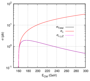
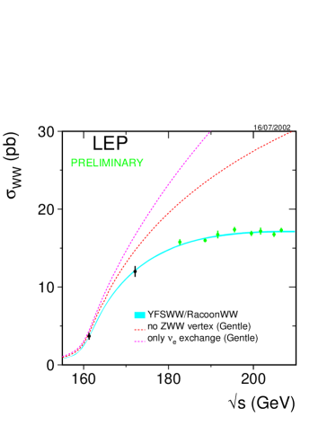
Figure 11: On the left panel it is shown the total cross section for $e^{-}+e^{+}\rightarrow W^{-}_{L}+W^{+}_{L}$ (black). Also shown are the $\nu$ exchange cross section (red) and the sum of the $\nu$ exchange with the s-channel exchange of gauge bosons (magenta). On the right panel it is shown the LEP result for $e^{-}+e^{+}\rightarrow W^{-}+W^{+}$.

At these energies the contribution of the diagrams involving the Higgs boson is very small, due to the smallness of the cross section the electron mass and can be completed neglected at LEP energies. One can estimate that the importance of the Higgs boson diagrams will show up when

$$\frac{m_{e}\sqrt{s}}{M_{W}^{2}}\simeq 1,\rightarrow\sqrt{s}\simeq 10^{7}\text{GeV}$$ (52)

an energy completely outside the reach of man-made accelerators. However, from the consistency point of view, the cancellation of the bad behavior at those energies should be there. This is shown in Fig. 12. Here we show the contribution of the various pieces to the cross section of the process $e^{-}+e^{+}\rightarrow W^{-}_{L}+W^{+}_{L}$. The total cross section is shown in black, the neutrino exchange in red and the sum of the neutrino with the gauge bosons in magenta. In blue is the contribution from the Higgs boson exchange. We see that for high enough energy, $\sqrt{s}\simeq M_{W}^{2}/m_{e}\simeq 10^{7}$ GeV, the Higgs boson contribution is crucial to avoid the cross section to be constant. If the electron mass was not so small, the effect would be seen much earlier as in the case of $W^{-}_{L}+W^{+}_{L}\rightarrow W^{-}_{L}+W^{+}_{L}$.

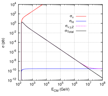
Figure 12: Various contributions to the cross section $e^{-}+e^{+}\rightarrow W^{-}_{L}+W^{+}_{L}$ at very high energy. See text for details.

IV.4 Other Polarizations of the $W$’s

As a last exercise let us calculate the cross sections for various final polarizations of the $W$ bosons. First, let us look at the total cross sections for the various possibilities. This is shown in Fig. 13, confirming what we said before concerning the relative importance of the various polarizations. On the right panel of that figure we show LEP results for comparison.

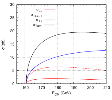
Figure 13: Cross section $e^{-}+e^{+}\rightarrow W^{-}+W^{+}$ for various polarizations of the final $W$ bosons. See text for details.

One can also learn something from the angular distributions of the differential cross sections. These are shown in Fig. 14 for two values of the center of mass energy, the first one close to threshold, the second one close to the maximum of the cross section.

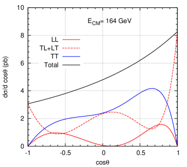
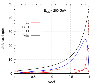
Figure 14: Angular dependence of the differential cross section for two values of the center of mass energy.

The more relevant fact is that the cross section is peaked in the forward direction and this feature increases with increasing beam energy. The other relevant piece of information has to do with the fact that for $\theta=0$, meaning the $W^{-}$ in the same direction as the incident electron, both the TT and LL differential cross section vanish, while the TL+LT has a maximum. This can be understood as follows. Due to the (V-A) nature of the charged current interaction, the electron will have helicity $-1/2$ while the positron helicity $+1/2$, resulting in a total helicity $-1$ in the direction of the electron. So if the $W$ bosons are produced in the same direction their total helicity must be $-1$ and that can only be achieved if one is transverse and the other longitudinal polarization, more precisely,

$$W^{-}(\lambda=-1),W^{+}(\lambda=0),\quad\text{or}\quad W^{+}(\lambda=+1),W^{-}(\lambda=0)$$ (53)

IV.5 Precision and speed: Mathematica, FORM and Fortran

In the previous discussion the more experienced reader should have been a bit puzzled. To make the point, let us enlarge the plot of Fig. 12. This is shown in the left panel of Fig. 15.

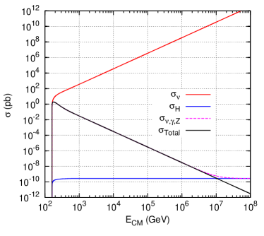
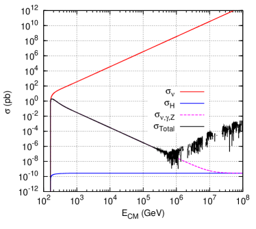
Figure 15: left panel: Same as in Fig. 12 but with a larger scale.

We see that for $\sqrt{s}=10^{7}$ GeV the cancellation has to be achieved better than one part in $10^{20}$. For numerical calculations in double precision in C or Fortran this is a problem. How come that we could achieve this precision without resorting to quadrupole precision?. The key to the answer lies in the fact that our formula for the total cross section already has the bad behaviour cancelled before we insert it into the Fortran program. This is achieved with Mathematica. One could think that this makes Mathematica a better choice to make the calculation of $|\mathcal{M}|^{2}$. However Mathematica is quite slow when compared with, for instance, FORM. For this problem in an Intel Core-2 at 2.56 MHz, it takes close to 350 s. The same problem with FORM takes less than 7 s, a factor of 50!. For larger problems, one has to use FORM. The problem with FORM is that has poor capabilities for simplifying expressions. So with FORM we can get (in 7 s) a Fortran output that is the sum of the all the contributions to $|\mathcal{M}|^{2}$ without great simplification. If we use this output we get the situation in the right panel of Fig. 15. The precision problems appear exactly where they should, at 1 part in $10^{13}$. But we can get the best of both programs, we can use FORM to evaluate the traces and input it into Mathematica to simplify the expressions and make a Fortran output. In this way we can get the same result as with Mathematica with a total time of around 20 s instead of 350 s! The whole process can be automatized ctqft:2007 .

V Conclusions

We have discussed the importance of the Higgs boson in making the SM consistent. We have used symbolic calculations with the package FeynCalc for Mathematica. The programs can be found at the web page in Ref.ctqft:2007 .

Appendix A Inputs for FeynCalc

A.1 $\nu_{e}+\overline{\nu}_{e}\rightarrow W^{+}_{L}+W^{-}_{L}$

We show here the code for the package FeynCalc that was used in section II.

(******************************** Program nunuWLWL.m ************************************* This program evaluates the amplitudes and cross section for the process

nu + nubar -¿ W^+_L + W^-_L

Author: Jorge C. Romão email: jorge.romao@ist.utl.pt ********************************* Program nunuWLWL.m ************************************) Remove[”Global‘*”]

dm[mu_] := DiracMatrix[mu] dm[5] := DiracMatrix[5] ds[p_] := DiracSlash[p] mt[mu_, nu_] := MetricTensor[mu, nu] fv[p_, mu_] := FourVector[p, mu] epsilon[a_, b_, c_, d_] := LeviCivita[a, b, c, d] id[n_] := IdentityMatrix[n] sp[p_, q_] := ScalarProduct[p, q] li[mu_] := LorentzIndex[mu] prop[p_, m_] := ds[p] + m

PVL[Q_,mu_]:= FourVector[Q,mu]

V[a_,b_,mu_,p_,k_,q_]:=mt[a,b] fv[p-k,mu] + mt[b,mu] fv[k-q,a] +  mt[mu,a] fv[q-p,b] PL=dm[7] PR=dm[6]

(* Functions *) TakeLimit=Function[exp, aux1=exp /. highenergy; aux2= aux1 /. x-¿1/z;  aux3=Normal[Series[aux2,z,0,0]]; aux4=Expand[aux3 /. z-¿1/x]]

CoefA=Function[exp,Coefficient[TakeLimit[exp],x,2]] CoefB=Function[exp,Coefficient[TakeLimit[exp],x,1]] CoefC=Function[exp,Coefficient[TakeLimit[exp],x,0]]

WriteMandel=Function[exp, TmpAux1 = exp /. onshell;  TmpAux2=Simplify[TmpAux1 /.ct]; Simplify[TmpAux2 /. beta-¿Sqrt[1-4 MW^2/s]]] ;

WriteTeX=Function[exp, TmpAux1 = WriteMandel[exp]; TmpAux2=TeXForm[TmpAux1]]

(* incoming: p1=nu, p2=nubar outgoing: q1=W+, q2=W- *)

onshell1=sp[p1,p1]-¿0,sp[p2,p2]-¿0,sp[q1,q1]-¿MW^2,sp[q2,q2]-¿MW^2 onshell2=sp[Q1,q1]-¿0,sp[Q2,q2]-¿0 onshell3=sp[Q1,p1]-¿s/4/MW (beta - cteta),sp[Q1,p2]-¿s/4/MW (beta + cteta), sp[Q1,q2]-¿s/2/MW beta,sp[Q2,p1]-¿s/4/MW (beta + cteta), sp[Q2,p2]-¿s/4/MW (beta - cteta),sp[Q2,q1]-¿s/2/MW beta onshell4=sp[Q1,Q1]-¿-1,sp[Q2,Q2]-¿-1 onshell5=sp[Q1,Q2]-¿s/4/MW^2 (beta^2 +1) onshell=Flatten[onshell1,onshell2,onshell3,onshell4,onshell5]

(****************************************************************************************) mandel=sp[p1,p2]-¿ s/2,sp[q1,q2]-¿ (s -2 MW^2)/2, sp[p1,q1]-¿ (MW^2 -t)/2, sp[p2,q2]-¿ ( MW^2-t)/2, sp[p1,q2]-¿ (s+t- MW^2)/2,sp[p2,q1]-¿ (s+t- MW^2)/2

highenergy=s-¿4 MW^2 x,t-¿ MW^2 (1 - 2 x (1- Sqrt[(1 -1/x)] cteta)),beta-¿Sqrt[1-1/x] weakangle=sw^2-¿1 -cw^2

ct = Part[Solve[t == MW^2 - s/2*(1 - beta*cteta), cteta], 1]

ampsZ= - 1/2 PVL[Q1,mu] PVL[Q2,nu] Spinor[-p2] . dm[a] . PL . Spinor[p1] V[mu,nu,b,-q1,-q2,q1+q2] (-mt[a,b] + fv[p1+p2,a] fv[p1+p2,b]/MW^2)/(s-MW^2/cw^2)

MsZ = Simplify[DiracSimplify[Contract[ampsZ] /. onshell] /. mandel]

ampNeu= - 1/2 Spinor[-p2] . dm[nu] . PL . prop[p1-q1,0] . dm[mu] . PL . Spinor[p1] PVL[Q1,mu] PVL[Q2,nu] 1/t

MtNeu= Simplify[DiracSimplify[Contract[ampNeu] /. onshell] /. mandel]

diracsub1=DiracGamma[Momentum[Q1]]-¿1/MW DiracGamma[Momentum[q1]], DiracGamma[Momentum[Q2]]-¿1/MW DiracGamma[Momentum[q2]];

diracsub2=Spinor[-Momentum[p2], 0, 1] . (DiracGamma[Momentum[q1]]/MW) . DiracGamma[7] . Spinor[Momentum[p1], 0, 1]-¿ 1/MW Spinor[-Momentum[p2], 0, 1] . DiracGamma[Momentum[q1]] . DiracGamma[7] . Spinor[Momentum[p1], 0, 1],Spinor[-Momentum[p2], 0, 1] . (DiracGamma[Momentum[q2]]/MW) . DiracGamma[7] . Spinor[Momentum[p1], 0, 1]-¿ 1/MW Spinor[-Momentum[p2], 0, 1] . DiracGamma[Momentum[q2]] . DiracGamma[7] . Spinor[Momentum[p1], 0, 1];

diracsub3=DiracGamma[Momentum[q2]]-¿DiracGamma[Momentum[p1+p2-q1]]

MsZaux1= MsZ /. diracsub1 MsZaux2= Simplify[MsZaux1 /. diracsub2] MsZaux3= MsZaux2 /. highenergy MsZaux4= MsZaux3 /. x-¿1/z MsZaux5= Normal[Series[MsZaux4,z,0,1]]

MtNeuaux1 = DiracSimplify[MtNeu /. diracsub1] MtNeuaux2 = MtNeuaux1 /. onshell MtNeuaux3 = MtNeuaux2 /. highenergy MtNeuaux4 = MtNeuaux3 /. x-¿1/z MtNeuaux5 = Normal[Series[MtNeuaux4,z,0,1]]

Mtotal= Simplify[MsZaux5 + MtNeuaux5]

MHighEnergy:= Simplify[DiracSimplify[Mtotal /. diracsub3] /. z-¿1/x]

Print[”1) High Energy Behaviour of the Amplitudes: x=s/(4 MW^2) ,

$$CurlyPhi](-p2).(\text{Gamma]CenterDot]q1).Gamma]7.CurlyPhi](p1)goeslikes"]Print["MHighEnergy=",MHighEnergy]{boxedverbatim}(∗∗∗∗∗∗∗∗∗∗∗∗∗∗∗∗∗∗∗∗∗∗∗∗∗∗∗∗∗∗∗}$$

References

- (1) C. Quigg, Gauge theories of strong, weak and alectromagnetic interactions (Addison-Wesley, New York, 1983).
- (2) J. C. Romão, Introdução à Teoria do Campo (IST, 2016), Available online at http://porthos.ist.utl.pt/ftp/textos/itc.pdf.
- (3) J. C. Romao, http://porthos.ist.utl.pt/CTQFT/ .
- (4) http://www.idpasc.lip.pt/ .