Study of GRB light curve decay indices in the afterglow phase

Abstract

In this work we study the distribution of temporal power-law decay indices, $\alpha$, in the Gamma Ray Burst (GRB) afterglow phase, fitted for $176$ GRBs (139 long GRBs, 12 short GRBs with extended emission and 25 X-Ray Flashes (XRFs)) with known redshifts. These indices are compared with the temporal decay index, $\alpha_{W}$, derived with the light curve fitting using the Willingale et al. [2007] model. This model fitting yields similar distributions of $\alpha_{W}$ to the fitted $\alpha$, but for individual bursts a difference can be significant. Analysis of ($\alpha$, $L_{a}$) distribution, where $L_{a}$ is the characteristic luminosity at the end of the plateau, reveals only a weak correlation of these quantities. However, we discovered a significant regular trend when studying GRB $\alpha$ values along the Dainotti et al. [2008] correlation between $L_{a}$ and the end time of the plateau emission in the rest frame, $T_{a}^{*}$, hereafter LT correlation. We note a systematic variation of the $\alpha$ parameter distribution with luminosity for any selected $T_{a}^{*}$. We analyze this systematics with respect to the fitted LT correlation line, expecting that the presented trend may allow to constrain the GRB physical models. We also attempted to use the derived correlation of $\alpha(T_{a})$ versus $L_{a}(T_{a})$ to diminish the luminosity scatter related to the variations of $\alpha$ along the LT distribution, a step forward in the effort of standardizing GRBs. A proposed toy model accounting for this systematics applied to the analyzed GRB distribution results in a slight increase of the LT correlation coefficient.

12pt,pra,apsrevtex4-1

1. Introduction

Gamma Ray Bursts (GRBs) with their powerful emission processes are observed up to high redshifts, $z>9$ [Cucchiara et al. , 2011]. A significant progress in studying GRB observations has been the advent of Swift satellite [Gehrels et al. , 2004], which has revealed a more complex behavior of the light curves [O’Brien et al. , 2006, Nousek et al. , 2006, Zhang et al. , 2006, Sakamoto et al. , 2007] than in the past. There are several emission models proposed in the literature providing predictions for characteristic GRB light curve features. Well known is the model of Meszaros [1998], Meszaros & Rees [1999], Meszaros [2006], consisting of jet internal shocks generating the GRB prompt phase emission and external shocks of the GRB expanding fireball generating the afterglow emission.

In the present paper we study distributions of the GRB afterglow parameters versus light curve temporal decay indices $\alpha$, for the power-law decay observed in the afterglow phase, with the X-ray luminosity $L_{a}$. We analyze an extended sample of 176 GRBs with known redshifts observed by Swift from January 2005 to July 2014. In the presented analysis we use the LT correlation [Dainotti et al. , 2008], updated in Dainotti et al. [2010, 2011a, 2013a, 2015a], between the derived characteristic afterglow plateau luminosity, $L_{a}$, and time, $T_{a}^{*}$ (an index * indicates the GRB rest frame quantity). An attempt to study similar afterglow properties was presented by Gendre et al. [2008]. They analyzed the “late” light curve properties at the time of 1 day after the burst to reveal existence of grouping the GRB luminosities into two groups which also differ in their redshift distributions. In their study they noted relations among some GRB parameters, in particular a non-trivial distribution of X-ray spectral indices versus the light curve temporal decay indices, but no dependence of these indices on the GRB luminosity. In addition, prompt-afterglow correlations have been studied by Dainotti et al. [2011b, 2015b], Margutti et al. [2013] and Grupe et al. [2013].

Importance of the present study results also from the fact that the afterglow LT correlation has already been the object of theoretical modeling either via accretion [Kumar et al. , 2008, Lindner et al. , 2010, Cannizzo & Gehrels , 2009, Cannizzo et al. , 2011], via a magnetar model [Dall’Osso et al. , 2011, Bernardini et al. , 2011, Rowlinson & O’Brien , 2012, Rowlinson et al. , 2013, 2014, Rea et al. , 2015] or energy injection [Sultana et al. , 2013, Leventis et al. , 2014, van Eerten , 2014a, b] and there were attempts to apply it as a cosmological tool [Cardone et al. , 2009, 2010, Dainotti et al. , 2013b, Postnikov et al. , 2014]. Here, we extend the LT correlation study looking into its possible dependence on the additional physical parameter $\alpha$ characterizing the afterglow light curve.

Below, in Section 2 we introduce the data set analyzed in this study. In Section 3 we describe the performed observational data analysis and the derived distributions of decay indices $\alpha$. The analysis reveals a weak correlation for $\alpha$ and $L_{a}$, but a significant systematic trend along the correlated ($L_{a}$, $T_{a}^{*}$) distribution. In Section 4 we present final discussion and conclusions. We shortly consider physical interpretation of the $\alpha$ distribution. Then, we preliminary explore a new possibility of using GRBs as cosmological standard candles, illustrated with a proposed toy model involving scaling GRB afterglow luminosity to the selected standard $\alpha_{0}$.

The fitted slopes and normalization parameters of the correlations presented in this paper are derived using the D’Agostini [2005] method. The $\Lambda$CDM cosmology applied here uses the parameters $H_{0}=71\ km\ s^{-1}\ Mpc^{-1}$, $\Omega_{\Lambda}=0.73$ and $\Omega_{M}=0.27$ .

2. Data Sample

Below, we analyze distribution of afterglow light curve decay indices, $\alpha$, for the data set of 176 GRBs with known redshifts, observed by Swift from January 2005 to July 2014. Within this sample we consider separately subsamples of 139 long GRBs, 25 X-Ray Flashes (XRFs), 12 short GRBs with extended emission. The sample of 164 long GRBs and XRFs is also considered together as a single sample.

As described in Dainotti et al. [2013a], all the analyzed light curves were fitted using an analytic functional form proposed by Willingale et al. [2007]. The considered sample was chosen from all Swift GRBs with known redshifts by selecting only those events which allowed a reliable afterglow fitting. The fits provided physical parameters for the GRB afterglows, including its characteristic luminosity and time, $L_{a}$ and $T_{a}^{*}$, at the end of the afterglow plateau phase, and the power-law temporal decay index, $\alpha_{W}$, for the afterglow decaying phase. The fitted indices $\alpha_{W}$ are influenced by the requirement of the best global light curve fitting for the considered analytic model. Therefore, we decided to apply a different procedure for the derivation of the temporal decay index $\alpha$ to be used in the following analysis, intended to provide a more accurate fit of the light curve power-law decay part immediately after the plateau. In each GRB we selected the afterglow light curve section with a power-law and we performed the $\chi^{2}$ fitting of $\alpha$ in such a range, as presented in the ON LINE MATERIAL including a set of figures for all GRBs showing the performed fits and providing the fitting parameters in the table. We compared these parameters with those by Evans et al. [2009] and the ones quoted in the Swift Burst Analyser (http://www.swift.ac.uk/burst_-analyser/), having nearly the same $\alpha$ values in the majority of cases. However, also significant differences are found in individual cases due to the different time ranges considered for the fits.

The applied procedure allowed to remove all clear deviations of the power-law from the fitting due to flares and non-uniformities in the observational data. In the case of a break in the decaying part of the light curve, a value of $\alpha$ was fitted to the brighter/earlier part of the light curve. We have to note that in some rare cases it was impossible to decide if the first part of the light curve can be considered the decaying part, or still a steep plateau phase, and the presented fits can be disputed. We decided to use all derived data in the analysis and correlations studied in this paper, leaving possibility of some particular data selection and/or rejecting some events from the analysis to the future study.

Comparison of the $\alpha$ and $\alpha_{W}$ distributions in Fig. 1 shows that both measured decay indices have similar distributions, but differences for individual fitted values can be significant. The parameters of the Gaussian fits for both presented distributions are: a mean value $\mu\left(\alpha\right)=1.40$ with standard deviation $\sigma\left(\alpha\right)=0.46$ for our power-law fitting compared to $\mu\left(\alpha_{W}\right)=1.45$ and $\sigma\left(\alpha_{W}\right)=0.45$ for the Willingale model fitting. The P-value of the T-test between these two distributions is 0.89, indicating no statistically significant differences between the two distributions.

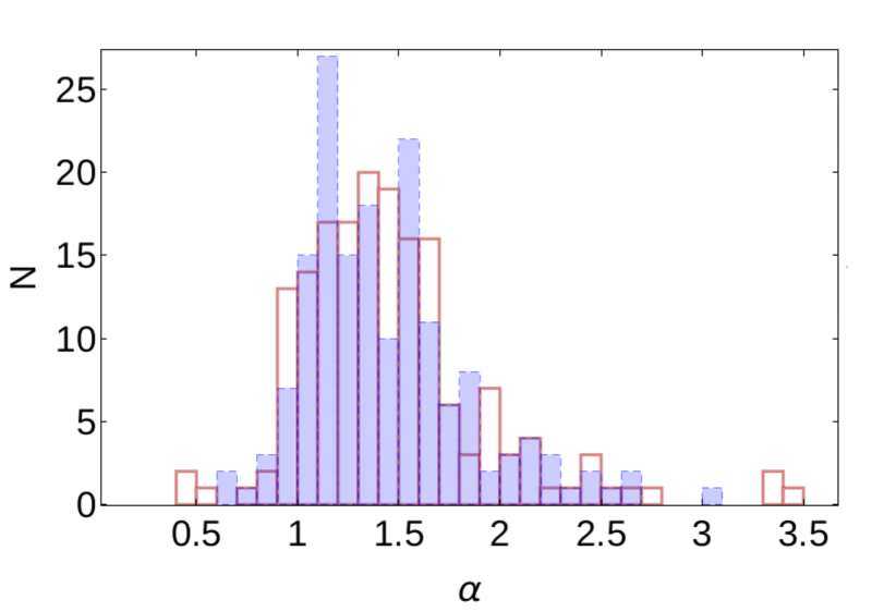
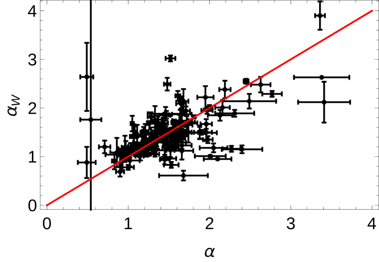
Figure 1.— Comparision of the derived indices $\alpha$ and $\alpha_{W}$. Upper panel: histograms of fitted $\alpha$ (solid red line) and $\alpha_{W}$ (shaded area). Bottom panel: the $\alpha_{W}$ versus $\alpha$ distribution. The red line $\alpha=\alpha_{W}$ is provided for reference.

3. Analysis of the afterglow decay light curves

By adopting the analyzed subsample of long GRBs+XRFs, systematic trends in the ($\log L_{a}$, $\alpha$) distribution can be studied. As presented in Fig. 2, there is an indication that these quantities are (weakly) correlated. However, scatter of points around the correlation line is substantial and the derived Spearman [Spearman , 1904] correlation coefficient $\rho=0.17$ is small. The fitted correlation line is $\log L_{a}$ = $0.30\,\alpha$ + $47.20$, showing that on average faster light curve decay seems to occur for GRBs with higher luminosities. However, here we stress again, the trend is weak in this highly scattered distribution. The same analysis using the long GRBs subsample only leads to a slightly weaker correlation with $\rho=0.14$ and $P=10^{-4}$.

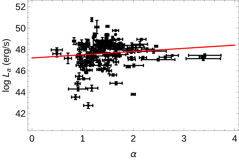
Figure 2.— Distribution of $\log L_{a}$ versus $\alpha$ for the long GRBs+XRFs subsample. The line presents a fitted weak correlation.

It should be noted that the large scatter of the GRB luminosity distribution can not be due only to the fitting method used for its derivation. Significant contribution to this scatter must result from the very nature of the GRB sources, possibly modified by the explosion geometry.

In the attempt to evaluate the trend in Fig. 2 we decided to compare distributions of $\alpha$ plotted for three luminosity ranges with equal numbers of GRBs: a low luminosity range – $\log L_{a}<47.25$, a medium range – $47.25<\log L_{a}<48.2$ , and a high range – $\log L_{a}>48.2$. Normalized cumulative distributions function $CDF$ ( $CDF(x)\equiv\sum_{0}^{x}(1/N)$, where summing includes all GRBs with $\alpha<x$ and $N$ is the number of GRBs in the considered sample) approximates the cumulative probability function in the $\alpha$ space. Below, in Fig. 3 we present these functions in the 3 analyzed luminosity ranges for the whole GRBs sample, as well as for long GRBs, short GRBs and XRFs subsamples. Comparison of the red and blue CDF distributions presented in Fig. 3 convincingly (maybe less convincingly for the short subsample) supports the existence of the ($\log L_{a}$, $\alpha$) correlation. The same systematics for all analyzed GRB samples with lower luminosity events show tendency to slower light curve decay. The most luminous GRBs (blue lines) seem to grow faster to unity with their smaller $\alpha$ scatter. This result is also confirmed by the Kolmogorov-Smirnov (KS) test. The test applied for low (red line) and high (blue line) luminosity GRB distributions along the $\alpha$ coordinate (Fig. 4) shows that it is highly unlikely, with $P=0.01$, that both distributions are drawn randomly from the same population. As regards the XRFs and short GRBs subsamples, the available number of elements is too low for establishing reliable statistical results, however the distributions of brighter GRBs seem to show the same tendency to be centered at higher $\alpha$ values than the dimmer ones.

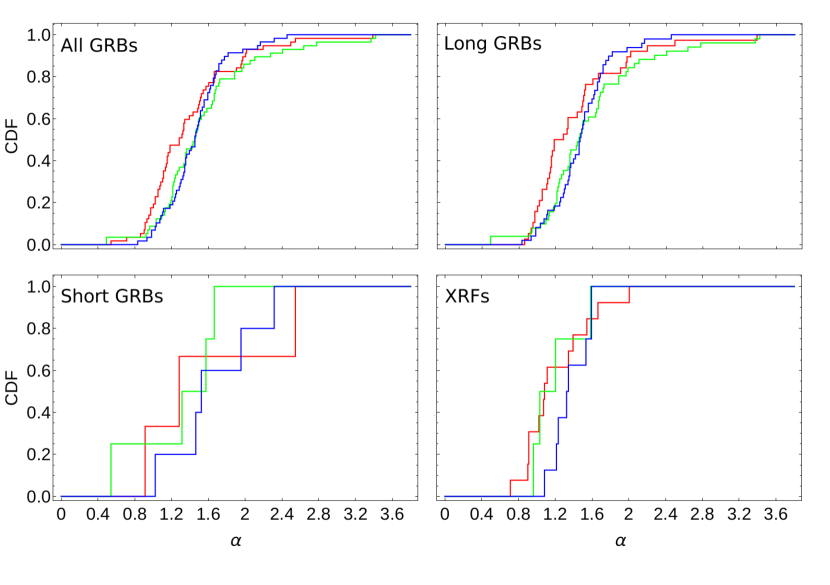
Figure 3.— Normalized cumulative distribution functions, $CDF$, versus $\alpha$ for the analyzed GRB subsamples in 3 considered luminosity ranges: $\log L_{a}<47.25$ (red), $47.25<\log L_{a}<48.2$ (green) and $\log L_{a}>48.2$ (blue).

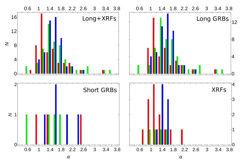
Figure 4.— GRB distributions of $\alpha$ for the analyzed subsamples in 3 considered luminosity ranges: $\log L_{a}<47.25$ (red), $47.25<\log L_{a}<48.2$ (green) and $\log L_{a}>48.2$ (blue). In each $\Delta\alpha$ bin the data for the different luminosity ranges are plotted as (shifted within the considered bin) separate color bars.

There is no well understood universal recipe yet for differentiating the physical properties of the GRB source from observational data, but the existence of $\log L_{a}$ versus $\log T_{a}^{*}$ correlation reflects the presence of $\sim$ uniformly varying properties of GRB progenitor in the plateau phase. If these properties would be the GRB progenitor mass and/or its angular momentum, then different external medium profiles could be expected around the exploding massive star, where the afterglow related shock propagates. Therefore, it may be expected to detect more clear dependence between the afterglow luminosity and the $\alpha$ index for GRBs analyzed within a limited range of $T_{a}^{*}$. To proceed, in analogy to the above analysis for selected luminosity ranges, we study relative distributions of GRB subsamples along the LT distribution in three ranges of the decay index: the “slowly” decaying light curves with $0.53<\alpha<1.23$, the “intermediate” ones with $1.23<\alpha<1.54$ and the “fast” decaying light curves with $1.54<\alpha<3.41$. With such selection each subsample has the same size.

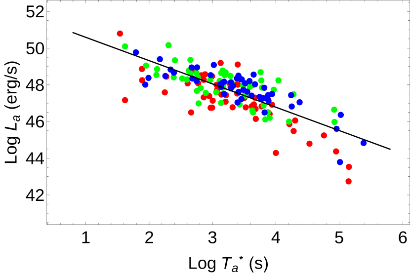
Figure 5.— Distribution of the long GRBs+XRFs subsample on the ($\log L_{a}$, $\log T_{a}^{*}$) plane for the three selected $\alpha$ subsamples: $0.53<\alpha<1.23$ (red), $1.23<\alpha<1.54$ (green) and $1.54<\alpha<3.41$ (blue). The black line represents the LT correlation line fitted for all presented GRBs.

Inspection of Fig. 5, presenting the considered long GRBs+XRFs $\alpha$-subsamples distributed along the LT correlation line, clearly reveals separation among these distributions. This behavior is also well visible in the normalized cumulative distribution functions plotted in Fig. 6. In particular, in Fig. 6 the considered samples (all, long GRBs and long GRBs+XRFs) are presented with respect to the ratio of the GRB afterglow luminosity $L_{a}(T_{a}^{*})$ to the respective luminosity $L_{LT}(T_{a}^{*})$ at the fitted correlation line: in the logarithmic scale $\log(L_{a}/L_{LT})$ = $\log L_{a}$ - $\log L_{LT}$ . A significant trend between the relative luminosity, $\log(L_{a}/L_{LT})$, and $\alpha$ is visible in Fig. 7, leading, e.g. to negligible KS probability, $P=1.4\times 10^{-6}$, that the low and high $\alpha$ subsamples are randomly drawn from a single GRB population.

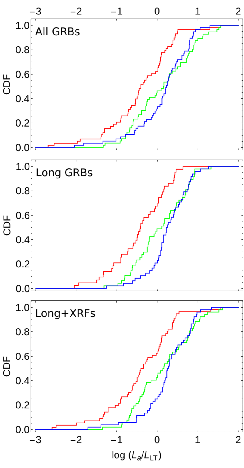
Figure 6.— Normalized cumulative distributions function $CDF$ versus $\log(L_{a}/L_{LT})$ for the analyzed GRB subsamples in 3 considered $\alpha$ ranges: $0.53<\alpha<1.23$ (red), $1.23<\alpha<1.54$ (green) and $1.54<\alpha<3.41$ (blue).

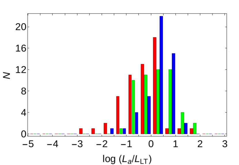
Figure 7.— Distributions of $\log(L_{a}/L_{LT})$ for the long GRBs+XRFs subsamples, for the three $\alpha$ ranges: $0.53<\alpha<1.23$ (red), $1.23<\alpha<1.54$ (green) and $1.54<\alpha<3.41$ (blue).

In Fig. 8 we present the distribution of $\log(L_{a}/L_{LT})$ versus the $\alpha$ index for the long GRBs+XRFs subsample. A linear fit for this distribution is

$$\log L_{a}-\log L_{LT}=(0.49\pm 0.17)\,\alpha-(0.70\pm 0.25)\quad,$$ (1)

with Spearman correlation coefficient $\rho=0.36$, and the probability for random occurrence $P=10^{-10}$. Using the long GRB subsample only, the correlation has a slightly smaller slope (0.42) with $\rho=0.36$ and $P=7.7\times 10^{-10}$. This correlation shows the observed tendency – with respect to the LT correlation line – for higher afterglow luminosity to have steeper light curve decay.

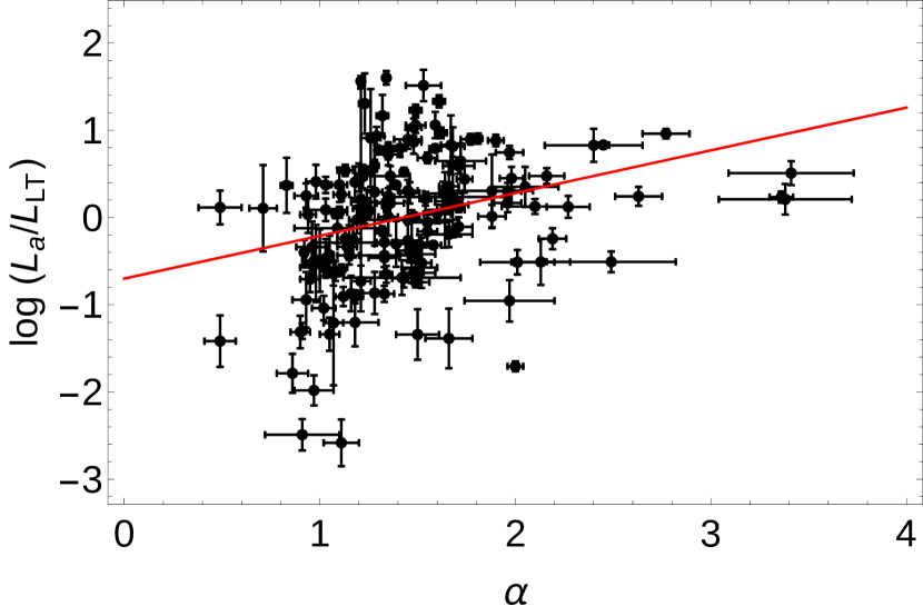
Figure 8.— Distribution of the long GRBs+XRFs subsample on the ($\alpha$, $\log(L_{a}/L_{LT})$) plane. The red line presents the fitted correlation (See Eq. 1).

To better evaluate the errors of the parameters fitted for the analyzed GRB sample, we decided to perform an additional statistical analysis using the Monte Carlo modeling of the data with $3\cdot 10^{4}$ simulations in each case. For each GRB we consider parameters $L_{a}$, $T_{a}^{*}$, and $\alpha$ to have Gaussian distributions around the fitted values, with the distribution width given by the respective 1 $\sigma$ uncertainty. Then, we randomly selected from the considered GRB sample - using a bootstrap procedure - the samples to be analyzed, where each GRB parameter was drawn from the respective Gaussian distribution. For each randomly created data sample we derived the correlation coefficient and the correlation slope by fitting the respective correlation $\log(L_{a}/L_{LT})$ vs. $\alpha$. As presented in the upper panels of Fig. 9, the simulations fully confirm reality of the derived correlation. We find that within the measurement errors existing correlation coefficient should be approximately between $0.2<\rho<0.5$ (mean value 0.35) and the fitted $\log(L_{a}/L_{LT})$ vs. $\alpha$ correlation should have an inclination $0.3<a<0.5$ (mean value 0.41), in agreement with the fitted errors in Eq. (1).

Using similar simulations as above, it can also be independently checked the possibility of randomly obtaining the studied $\log(L_{a}/L_{LT})$ vs. $\alpha$ correlation if no systematic relation of $\alpha$ in respect to $L_{a}$ and $T_{a}^{*}$ exists. We performed such analysis by randomly drawing samples using the procedure above, again within the bootstrap scheme, but with separately drawing pairs of parameters $L_{a}$ and $T_{a}^{*}$ from the GRB sample, and the $\alpha$ values from the sample of these values for the considered GRBs. Such procedure removes any correlation between $\alpha$ and other GRB parameters in the sample and shows that the possibility of randomly obtaining the correlation coefficient found in the real data is negligible (Fig. 9, lower panels).

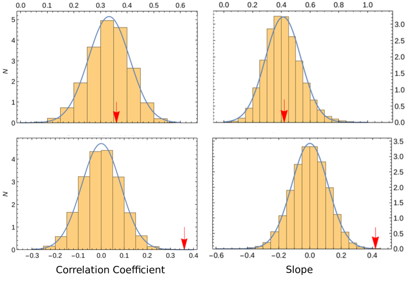
Figure 9.— The results of the Monte Carlo simulations for the long subsample: the normalized distributions of the correlation coefficient $\rho$ and the slope $a$ of the $\log(L_{a}/L_{LT})$ vs. $\alpha$ correlation for bootstrapped simulations including random data scatter within the measurement error ranges (upper panels) and the analogous distributions with the $\alpha$ parameters separately randomly drawn from the sample (lower panels). With red arrows we indicated values obtained in the above analysis of the original data.

4. Final discussion and Conclusions

Analysis of the fitted afterglow power-law temporal decay indices for the subsample of long GRBs+XRFs reveals a weak trend towards a steeper decay phase for higher afterglow luminosity $L_{a}$. The trend turns into a significant correlation if we consider GRB afterglow luminosity scaled to the one expected from the fitted LT correlation, for a given GRB afterglow plateau end time $T_{a}^{*}$. As different $T_{a}^{*}$ values result from varying properties of the GRB sources, the present analysis can be used to get new insight into physical nature of such sources.

4.1. Theoretical models

It is worth to note the attempts in the literature to provide physical interpretation of $\log L_{a}$ versus $\alpha$ relation. We can refer to such model presented by Hascoet et al. [2014] (see also Genet et al. [2007]) in order to relate the considered $\alpha$ parameter to the microphysics of the reverse shock emission. In the model of Hascoet et al. the energy deposition rate, ${\dot{E}}_{T}$, in the GRB afterglow, varied in time ‘$t$’ with a power-law dependence on the Lorentz gamma factor, $\Gamma(t)$:

$${\dot{E}}_{\rm T}(\Gamma(t))=\left\{\begin{array}[]{cl}{\dot{E}}_{*}\left(\frac{\Gamma(t)}{\Gamma_{*}}\right)^{-q}\ \ \ {\rm for}\ \ \Gamma(t)>\Gamma_{*}\\ {\dot{E}}_{*}\left(\frac{\Gamma(t)}{\Gamma_{*}}\right)^{q^{\,\prime}}\ \ \ {\rm for}\ \ \Gamma(t)<\Gamma_{*}\\ \end{array}\right.$$ (2)

where the energy scale ${\dot{E}}_{*}$ is determined by the total energy injected in the afterglow phase; $q$ and $q^{\,\prime}$ are the power-law indices for the time dependence of the energy injection rate. In this model the $q$ parameter constraints the shape of the plateau phase, while $q^{\,\prime}$ carries information about the light curve temporal decay index after the plateau. The characteristic value of $\Gamma_{*}$ sets the duration of the plateau. With the assumed power-law radial distribution of the medium surrounding the GRB progenitor, the Lorentz factor evolves as

$$\Gamma(t)=\Gamma_{*}\left(\frac{t}{T^{*}_{a}}\right)^{-\gamma},$$ (3)

where, e.g., $\gamma=3/8$ for a uniform medium and $\gamma=1/4$ for a stellar wind. Hascoet et al. derived the light curve temporal decay indices before ($\alpha_{1}$) and after ($\alpha_{2}$) the break at the end of the plateau phase as

$$\left\{\begin{array}[]{ll}\alpha_{1}=\gamma q-1\\ \alpha_{2}=-\gamma q^{\,\prime}-1\end{array}\right.$$ (4)

so that the flat plateau phase should be present for $q\approx 1/\gamma$, i.e. close to $q=8/3$ in the uniform medium and $q=4$ in the wind case. In the presented example Hascoet et al. [2014] considered the temporal decay index after the plateau $\alpha_{2}=-1.5$, leading to $q^{\,\prime}=1/(2\gamma)$ and the parameters of the central engine energy deposition in the late afterglow stage $q^{\,\prime}=4/3$ and 2, for the uniform medium and the wind case, respectively. It should be noted that this example uses the $\alpha_{2}$ value very close to the mean value of our distribution, $\alpha_{mean}=1.4\pm 0.3$, as visible in the upper panel of Fig. 1.

We should remark here that the observed large scatter in the $\alpha$ distribution seems to be difficult to be explained only by variations of the source radial density profile, influencing the shock propagation. Therefore, we consider the present discussion only as an example of the study based on the $\alpha$ parameter measurements.

4.2. GRB standardization

As the second aspect of the present study, we consider a possible usage of the measured afterglow light curve $\alpha$ for physically differentiating the observed GRBs. E.g., the revealed $\log(L_{a}/L_{LT})$ versus $\alpha$ correlation can be used to search for the procedure which could enable the standardization of GRBs and eventually to reveal a new cosmological standard candle. As an illustrative toy model, for such approach we introduce a procedure for GRBs resembling the one used for the standardization of SN Ia light curves by using the so called Phillips relation between the peak magnitude and the “stretching parameter” [Phillips , 1993]. In an attempt to scale GRBs with different temporal decay indices $\alpha$ to the standard source properties, we define the standard GRB as the one characterized by the value of the temporal decay index $\alpha_{0}=1.4$, approximately the mean value of the distribution presented in Fig. 1. Further, we postulate that the expected “standardized” GRB luminosity, $L_{a,0}$, can be derived using its measured decay index $\alpha$ and by scaling it to $\alpha_{0}$ using Eq. 1:

$$\log L_{a,0}=\log L_{a}+0.49\,(\alpha_{0}-\alpha)\quad.$$ (5)

This procedure applied for all the events in the analyzed subsample of long GRBs+XRFs results in only a slight increase in the LT correlation coefficient absolute value, from $\rho=-0.72$ for the original ($\log L_{a}$, $\log T_{a}^{*}$) data to $\rho_{0}=-0.76$ for the modified distribution ($\log L_{a,0}$, $\log T_{a}^{*}$). When using the long GRBs subsample only the increase in the correlation coefficient is even smaller. This increase in the correlation coefficient is obtained by the fits for quite different shapes of the afterglow light curves and thus different quality of available GRB parameters $L_{a}$, $T_{a}^{*}$ and $\alpha$. More detailed analysis of this standardization procedure, with careful consideration of the afterglow light curves for the selected events, is in progress now.

Acknowledgements. This work made use of data supplied by the UK Swift Science Data Centre at the University of Leicester. The work of RDV and MO was supported by the Polish National Science Centre through the grant DEC-2012/04/A/ST9/00083. M.G.D is grateful to the Marie Curie Program, because the research leading to these results has received funding from the European Union Seventh FrameWork Program (FP7-2007/2013) under grant agreement N 626267.

References

- Bevington & Robinson [2003] Bevington, P.R., & Robinson, D.K. (2003), Data reduction and error analysis for the physical sciences, 3rd ed. New York: McGraw-Hill.
- Bernardini et al. [2011] Bernardini, M.G., Margutti, R., Chincarini, G., Guidorzi, C., & Mao, J. (2011), Gamma-ray burst long lasting X-ray flaring activity, A&A, 526, A27.
- Cannizzo & Gehrels [2009] Cannizzo, J.K., & Gehrels, N. (2009), A New Paradigm for Gamma-ray Bursts: Long-term Accretion Rate Modulation by an External Accretion Disk, ApJ, 700, 1047.
- Cannizzo et al. [2011] Cannizzo, J.K., Troja, E., & Gehrels, N. (2011), Fall-back Disks in Long and Short Gamma-Ray Bursts, ApJ, 734, 35.
- Cardone et al. [2009] Cardone, V.F., Capozziello, S., & Dainotti, M.G. (2009), An updated gamma-ray bursts Hubble diagram, MNRAS, 400, 775.
- Cardone et al. [2010] Cardone, V.F., Dainotti, M.G., Capozziello, S., & Willingale, R. (2010), Constraining cosmological parameters by gamma-ray burst X-ray afterglow light curves, MNRAS, 408, 1181.
- Cucchiara et al. [2011] Cucchiara, A., Levan, A. J., Fox, D. B., Tanvir, N. R., Ukwatta, T. N., Berger, E., Krhler, T., Kpc Yoldas, A., Wu, X. F., Toma, K., Greiner, J., Olivares, F. E., Rowlinson, A., Amati, L., Sakamoto, T., Roth, K., Stephens, A., Fritz, Alexander, Fynbo, J. P. U., Hjorth, J., Malesani, D., Jakobsson, P., Wiersema, K., O’Brien, P. T., Soderberg, A. M., Foley, R. J., Fruchter, A. S., Rhoads, J., Rutledge, R. E., Schmidt, B. P., Dopita, M. A., Podsiadlowski, P., Willingale, R., Wolf, C., Kulkarni, S. R., D’Avanzo, P. (2001), A Photometric Redshift of for GRB 090429B, ApJ, 736, 7.
- D’Agostini [2005] D’Agostini, G. (2005), Fits, and especially linear fits, with errors on both axes, extra variance of the data points and other complications, arXiv:physics/0511182 [physics.data-an].
- Dainotti et al. [2008] Dainotti, M.G., Cardone, V.F., & Capozziello, S. (2008), A time- luminosity correlation for -ray bursts in the X-rays, MNRAS, 391, L79.
- Dainotti et al. [2010] Dainotti, M.G., Willingale, R., Capozziello, S., Cardone, V.F., & Ostrowski, M. (2010), Discovery of a Tight Correlation for Gamma-ray Burst Afterglows with ”Canonical” Light Curves, ApJ, 722, L215.
- Dainotti et al. [2011a] Dainotti, M.G., Cardone, V.F., Capozziello, S., Ostrowski, M., & Willingale, R. (2011a), Study of Possible Systematics in the L*X-T*a Correlation of Gamma-ray Bursts, ApJ, 730, 135.
- Dainotti et al. [2011b] Dainotti, M.G., Ostrowski, M., & Willingale, R. (2011b), Towards a standard gamma-ray burst: tight correlations between the prompt and the afterglow plateau phase emission, MNRAS, 418, 2202.
- Dainotti et al. [2013a] Dainotti, Maria Giovanna, Petrosian, Vahe’, Singal, Jack, & Ostrowski, Michal (2013a), Determination of the Intrinsic Luminosity Time Correlation in the X-Ray Afterglows of Gamma-Ray Bursts, ApJ, 774, 157.
- Dainotti et al. [2013b] Dainotti, M.G., Cardone, V.F., Piedipalumbo E., & Capozziello, S. (2013b), Slope evolution of GRB correlations and cosmology, MNRAS, 436, 82.
- Dainotti et al. [2015a] Dainotti, M. G., Del Vecchio, R., Nagataki, S., Capozziello, S. (2015a), Selection Effects in Gamma-Ray Burst Correlations: Consequences on the Ratio between Gamma-Ray Burst and Star Formation Rates, ApJ, 800, 31.
- Dainotti et al. [2015b] Dainotti, M, Petrosian, V., Willingale, R., O’Brien, P., Ostrowski, M., & Nagataki, S. (2015b), Luminosity-time and luminosity-luminosity correlations for GRB prompt and afterglow plateau emissions, MNRAS, 451, 3898.
- Dall’Osso et al. [2011] Dall’Osso, S., Stratta, G., Guetta, D., Covino, S., De Cesare, G., & Stella, L. (2011), Gamma-ray bursts afterglows with energy injection from a spinning down neutron star, A&A, 526, A121.
- Evans et al. [2009] Evans, P.A., Beardmore, A.P., Page, K.L., Osborne, J.P., O’Brien, P.T., Willingale, R., Starling, R.L.C., Burrows, D.N., Godet, O., Vetere, L., Racusin, J., Goad, M.R., Wiersema, K., Angelini, L., Capalbi, M., Chincarini, G., Gehrels, N., Kennea, J.A., Margutti, R., Morris, D.C., Mountford, C.J., Pagani, C., Perri, M., Romano, P., & Tanvir, N. (2009), Methods and results of an automatic analysis of a complete sample of Swift-XRT observations of GRBs, MNRAS, 397, 1177.
- Gehrels et al. [2004] Gehrels et al. (2004), The Swift Gamma-Ray Burst Mission, ApJ, 611, 1005.
- Gendre et al. [2008] Gendre, B., Galli, A. and Boër, M. (2008), X-ray afterglow light curves: toward a standard candle?, ApJ, 683, 620.
- Genet et al. [2007] Genet, F., Daigne, F., & Mochkovitch, R. (2007), Can the early X-ray afterglow of gamma-ray bursts be explained by a contribution from the reverse shock?, MNRAS, 381, 732.
- Grupe et al. [2013] Grupe, D., Nousek, J.A., Veres, P., Zhang, B.B., & Gehrels, N. (2013), Evidence for New Relations between Gamma-Ray Burst Prompt and X-Ray Afterglow Emission from 9 Years of Swift, ApJS, 209, 20.
- Hascoet et al. [2014] Hascoet, R., Daigne, F. & Mochkovitch R. (2014), The prompt-early afterglow connection in gamma-ray bursts: implications for the early afterglow physics, MNRAS, 442, 20.
- Ioka & Nakamura [2001] Ioka, K., & Nakamura, T. (2001), Peak Luminosity-Spectral Lag Relation Caused by the Viewing Angle of the Collimated Gamma-Ray Bursts, ApJ, 554, L163.
- Kumar et al. [2008] Kumar, P., Narayan, R., & Johnson, J.L. (2008), Properties of Gamma-Ray Burst Progenitor Stars, Science, 321, 376.
- Leventis et al. [2014] Leventis, K., Wijers, R.A.M.J., & van der Horst, A.J. (2014), The plateau phase of gamma-ray burst afterglows in the thick-shell scenario, MNRAS, 437, 2448.
- Lindner et al. [2010] Lindner, C.C., Milosavljević, M., Couch, S.M., & Kumar, P. (2010), Collapsar Accretion and the Gamma-Ray Burst X-Ray Light Curve, ApJ, 713, 800.
- Margutti et al. [2013] Margutti, R., Zaninoni, E., Bernardini, M.G., Chincarini, G., Pasotti, F., Guidorzi, C., Angelini, L., Burrows, D. N., Capalbi, M., Evans, P. A., Gehrels, N., Kennea, J., Mangano, V., Moretti, A., Nousek, J., Osborne, J.P., Page, K.L., Perri, M., Racusin, J., Romano, P., Sbarufatti, B., Stafford, S., & Stamatikos, M. (2013), The prompt-afterglow connection in gamma-ray bursts: a comprehensive statistical analysis of Swift X-ray light curves, MNRAS, 428, 729.
- Meszaros [1998] Mészáros, P. (1998), Theoretical models of gamma-ray bursts, American Institute of Physics Conference Series, Gamma-Ray Bursts 4th Hunstville Symposium, 428, 647.
- Meszaros [2006] Mészáros, P. (2006), Gamma-ray bursts, Reports on Progress in Physics, 69, 2259.
- Meszaros & Rees [1999] Meszaros, P. & Rees, M.J. (1999), GRB 990123: reverse and internal shock flashes and late afterglow behaviour, MNRAS, 306, L39.
- Nousek et al. [2006] Nousek, J. et al. (2006), Evidence for a Canonical Gamma-Ray Burst Afterglow Light Curve in the Swift XRT Data, ApJ, 642,389.
- O’Brien et al. [2006] O’Brien, P.T., Willingale, R., Osborne, J. et al. (2006), The Early X-Ray Emission from GRBs, ApJ, 647, 1213.
- Phillips [1993] Phillips, M. M. (1993), The absolute magnitudes of Type IA supernovae, ApJ, 413, L105.
- Postnikov et al. [2014] Postnikov, S., Dainotti, M.G., Hernandez, X., & Capozziello, S. (2014), Nonparametric Study of the Evolution of the Cosmological Equation of State with SNeIa, BAO, and High-redshift GRBs, ApJ, 783, 126.
- Rea et al. [2015] Rea, N., Gullón, M., Pons, J. A., Perna, R., Dainotti, M.G., Miralles, J. A.. & Torres, D. F. (2015), Constraining the GRB-Magnetar Model by Means of the Galactic Pulsar Population, ApJ, 813, 92.
- Rowlinson & O’Brien [2012] Rowlinson, A., & O’Brien, P. (2012), Energy injection in short GRBs and the role of magnetars, Gamma-Ray Bursts 2012 Conference (GRB 2012), 100.
- Rowlinson et al. [2013] Rowlinson, A., O’Brien, P.T., Metzger, B.D., Tanvir, N.R., & Levan, A.J. (2013), Signatures of magnetar central engines in short GRB light curves, MNRAS, 430, 1061.
- Rowlinson et al. [2014] Rowlinson, A., Gompertz, B.P., Dainotti, M.G., O’Brien, P.T., Wijers, R.A.M.J., & van der Horst, A.J. (2014), Constraining properties of GRB magnetar central engines using the observed plateau luminosity and duration correlation, MNRAS, 443, 1779.
- Sakamoto et al. [2007] Sakamoto, T., Hill, J., Yamazaki, R. et al. (2007), Evidence of Exponential Decay Emission in the Swift Gamma-Ray Bursts, ApJ, 669, 1115.
- Spearman [1904] Spearman, C. (1904), The proof and measurement of association between two things, Amer. J. Psychol., 15, 72.
- Sultana et al. [2013] Sultana, J., Kazanas, D., & Mastichiadis, A. (2013), The Supercritical Pile Gamma-Ray Burst Model: The GRB Afterglow Steep Decline and Plateau Phase, ApJ, 779, 16.
- van Eerten [2014a] van Eerten, H. (2014), Self-similar relativistic blast waves with energy injection, MNRAS, 442, 3495.
- van Eerten [2014b] van Eerten, H.J. (2014), Gamma-ray burst afterglow plateau break time-luminosity correlations favour thick shell models over thin shell models, MNRAS, 445, 2414.
- Willingale et al. [2007] Willingale, R., O’Brien, P.T., Osborne, J.P., Godet, O., Page, K.L., Goad, M.R., Burrows, D.N., Zhang, B., Rol, E., Gehrels, N., & Chincarini, G. (2007), Testing the Standard Fireball Model of Gamma-Ray Bursts Using Late X-Ray Afterglows Measured by Swift, ApJ, 662, 1093.
- Willingale et al. [2010] Willingale, R., Genet, F., Granot, J., & O’Brien, P. T. (2010), The spectral-temporal properties of the prompt pulses and rapid decay phase of gamma-ray bursts, MNRAS, 403, 1296.
- Yamazaki et al. [2002] Yamazaki, R., Ioka, K., & Nakamura, T. (2002) X-Ray Flashes from Off-Axis Gamma-Ray Bursts, ApJ, 571, L31.
- Zhang et al. [2006] Zhang et al. (2006), Physical Processes Shaping Gamma-Ray Burst X-Ray Afterglow Light Curves: Theoretical Implications from the Swift X-Ray Telescope Observations, ApJ, 642, 354.