Stability Analysis and Design of
Momentum-based Controllers for Humanoid Robots

Abstract

Envisioned applications for humanoid robots call for the design of balancing and walking controllers. While promising results have been recently achieved, robust and reliable controllers are still a challenge for the control community dealing with humanoid robotics. Momentum-based strategies have proven their effectiveness for controlling humanoids balancing, but the stability analysis of these controllers is still missing. The contribution of this paper is twofold. First, we numerically show that the application of state-of-the-art momentum-based control strategies may lead to unstable zero dynamics. Secondly, we propose simple modifications to the control architecture that avoid instabilities at the zero-dynamics level. Asymptotic stability of the closed loop system is shown by means of a Lyapunov analysis on the linearized system’s joint space. The theoretical results are validated with both simulations and experiments on the iCub humanoid robot.

I INTRODUCTION

Humanoid robotics is doubtless an emerging field of engineering. One of the reasons accounting for this interest is the need of conceiving systems that can operate in places where humans are forbidden to access. To this purpose, the scientific community has paid much attention to endowing robots with two main capabilities: locomotion and manipulation. At the present day, the results shown at the DARPA Robotics Challenge are promising, but still far from being fully reliable in real applications. Stability issues of both low and high level controllers for balancing and walking were among the main contributors to robot failures. A common high-level control strategy adopted during the competition was that of regulating the robot’s momentum, which is usually referred to as momentum-based control. This paper presents numerical evidence that momentum-based controllers may lead to unstable zero dynamics and proposes a modification to this control scheme that ensures asymptotic stability.

Balancing controllers for humanoid robots have long attracted the attention of the robotic community [1, 2]. Kinematic and dynamic controllers have been common approaches for ensuring a stable robot behavior for years [3],[4]. The common denominator of these strategies is considering the robot attached to ground, which allows one for the application of classical algorithms developed for fixed-based manipulators.

At the modeling level, the emergence of floating-base formalisms for characterizing the dynamics of multi-body systems has loosened the assumption of having a robot link attached to ground [5]. At the control level, instead, one of the major complexities when dealing with floating base systems comes from the robot’s underactuation. In fact, the underactuation forbids the full feedback linearization of the underlying system [6]. The lack of actuation is usually circumvented by means of rigid contacts between the robot and the environment, but this requires close attention to the forces the robot exerts at the contact locations. If not regulated appropriately, uncontrolled contact forces may break the contact, and the robot control becomes critical [7],[8].

Contact forces/torques, which act on the system as external wrenches, have a direct impact on the rate-of-change of the robot’s momentum. Indeed, the time derivative of the robot’s momentum equals the net wrench acting on the system. Furthermore, since the robot’s linear momentum can be expressed in terms of the center-of-mass velocity, controlling the robot’s momentum is particularly tempting for ensuring both robot and contact stability (see, e.g.,  [9] for proper definition of contact stability).

Several momentum-based control strategies have been implemented in real applications [10],[11],[12]. The essence of these strategies is that of controlling the robot’s momentum while guaranteeing stable zero-dynamics. The latter objective is often achieved by means of a postural task, which usually acts in the null space of the control of the robot’s momentum [13],[14],[15]. These two tasks are achieved by monitoring the contact wrenches, which are ensured to belong to the associated feasible domains by resorting to quadratic programming (QP) solvers [7],[8],[16]. The control of the zero-dynamics can also be used to control the robot joint configuration [15].

The control of the linear momentum is exploited to stabilize a desired position for the robot’s center of mass. In contrast, the choice of desired values for the robot angular momentum is still unclear [17]. Hence, control strategies that neglect the control of the robot’s angular momentum have also been implemented [18]. Controlling both the robot linear and angular momentum, however, is particularly useful for determining the contact torques, and it has become a common torque-controlled strategy for dealing with balancing and walking humanoids. Controlling also the angular momentum results in a more human-like behavior and better response to perturbations [19],[20].

To the best of the authors’ knowledge, the stability analysis of momentum-based control strategies in the contexts of floating base systems is still missing. The contribution of this paper goes along this direction by considering a humanoid robot standing on one foot, and is then twofold. First, we present numerical evidence that classical momentum-based control strategies may lead to unstable zero dynamics, thus meaning that classical postural tasks are not sufficient in these cases. The main cause of this instability is the lack of orientation correction terms at the angular momentum level: we show that correction terms of the form of angular momentum integrals are sufficient for ensuring asymptotic stability of the closed loop system, which is proved by means of a Lyapunov analysis. The postural control, however, is modified with respect to (w.r.t.) state-of-the-art choices. The validity of the presented controller is tested both in simulation and on the humanoid robot iCub.

This paper is organized as follows. Section II introduces the notation, the system modeling, and also recalls a classical momentum-based control strategy. Section III presents numerical results showing that momentum based control strategies for humanoid robots may lead to unstable zero dynamics. Section IV presents a modification of the momentum based control strategy for which stability and convergence can be proven. Section V discusses the numerical and experimental validation of the proposed approach. Conclusions and perspectives conclude the paper.

II BACKGROUND

II-A Notation

• $\mathcal{I}$ denotes an inertial frame, with its $z$ axis pointing against the gravity. The constant $g$ denotes the norm of the gravitational acceleration.

• $e_{i}\in\mathbb{R}^{m}$ is the canonical vector, consisting of all zeros but the $i$-th component that is equal to one.

• Given two orientation frames $A$ and $B$, and two vectors $\prescript{A}{}{p},\prescript{B}{}{p}\in\mathbb{R}^{3}$ expressed in these orientation frames, the rotation matrix $\prescript{A}{}{R}_{B}$ is such that $\prescript{A}{}{p}=\prescript{A}{}{R}_{B}\prescript{B}{}{p}$.

• Let $S(x)\in\mathbb{R}^{3\times 3}$ be the skew-symmetric matrix such that $S(x)y=x\times y$, where $\times$ is the cross product operator in $\mathbb{R}^{3}$.

• Given a function $f(x,y)\mathrel{\mathop{\mathchar 58\relax}}\mathbb{R}^{n}\times\mathbb{R}^{m}\rightarrow\mathbb{R}^{p}$, the partial derivative of $f(\cdot)$ w.r.t. the variable $x$ is denoted as $\partial_{x}f(x,y)=\frac{\partial f(x,y)}{\partial x}\in\mathbb{R}^{p\times n}$.

II-B Modelling

It is assumed that the robot is composed of $n+1$ rigid bodies, called links, connected by $n$ joints with one degree of freedom each. We also assume that the multi-body system is free floating, i.e. none of the links has an a priori constant pose with respect to the inertial frame. The robot configuration space can then be characterized by the position and the orientation of a frame attached to a robot’s link, called base frame $\mathcal{B}$, and the joint configurations. Thus, the configuration space is defined by $\mathbb{Q}=\mathbb{R}^{3}\times SO(3)\times\mathbb{R}^{n}$. An element of $\mathbb{Q}$ is then a triplet $q=(\prescript{\mathcal{I}}{}{p}_{\mathcal{B}},\prescript{\mathcal{I}}{}{R}_{\mathcal{B}},q_{j})$, where $(\prescript{\mathcal{I}}{}{p}_{\mathcal{B}},\prescript{\mathcal{I}}{}{R}_{\mathcal{B}})$ denotes the origin and orientation of the base frame expressed in the inertial frame, and $q_{j}$ denotes the joint angles. It is possible to define an operation associated with the set $\mathbb{Q}$ such that this set is a group. Given two elements $q$ and $\rho$ of the configuration space, the set $\mathbb{Q}$ is a group under the following operation: $q\cdot\rho=(p_{q}+p_{\rho},R_{q}R_{\rho},q_{j}+{\rho}_{j}).$

Furthermore, one easily shows that $\mathbb{Q}$ is a Lie group. Then, the velocity of the multi-body system can be characterized by the algebra $\mathbb{V}$ of $\mathbb{Q}$ defined by: $\mathbb{V}=\mathbb{R}^{3}\times\mathbb{R}^{3}\times\mathbb{R}^{n}$. An element of $\mathbb{V}$ is then a triplet $\nu=(^{\mathcal{I}}\dot{p}_{\mathcal{B}},^{\mathcal{I}}\omega_{\mathcal{B}},\dot{q}_{j})=(\text{v}_{\mathcal{B}},\dot{q}_{j})$, where ${}^{\mathcal{I}}\omega_{\mathcal{B}}$ is the angular velocity of the base frame expressed w.r.t. the inertial frame, i.e. ${}^{\mathcal{I}}\dot{R}_{\mathcal{B}}=S(^{\mathcal{I}}\omega_{\mathcal{B}})^{\mathcal{I}}{R}_{\mathcal{B}}$.

We also assume that the robot is interacting with the environment exchanging $n_{c}$ distinct wrenches. The application of the Euler-Poincaré formalism [21, Ch. 13.5] to the multi-body system yields the following equations of motion:

$${M}(q)\dot{{\nu}}+{C}(q,{\nu}){\nu}+{G}(q)=B\tau+\sum_{k=1}^{n_{c}}{J}^{\top}_{\mathcal{C}_{k}}f_{k}$$ (1)

where ${M}\in\mathbb{R}^{n+6\times n+6}$ is the mass matrix, ${C}\in\mathbb{R}^{n+6\times n+6}$ is the Coriolis matrix, ${G}\in\mathbb{R}^{n+6}$ is the gravity term, $B=(0_{n\times 6},1_{n})^{\top}$ is a selector matrix, $\tau\in\mathbb{R}^{n}$ is a vector representing the actuation joint torques, and $f_{k}\in\mathbb{R}^{6}$ denotes the $k$-th external wrench applied by the environment on the robot. We assume that the application point of the external wrench is associated with a frame $\mathcal{C}_{k}$, attached to the link on which the wrench acts, and has its $z$ axis pointing in the direction of the normal of the contact plane. Then, the external wrench $f_{k}$ is expressed in a frame whose orientation is that of the inertial frame $\mathcal{I}$, and whose origin is that of $\mathcal{C}_{k}$, i.e. the application point of the external wrench $f_{k}$. The Jacobian ${J}_{\mathcal{C}_{k}}={J}_{\mathcal{C}_{k}}(q)$ is the map between the robot’s velocity ${\nu}$ and the linear and angular velocity ${}^{\mathcal{I}}\text{v}_{\mathcal{C}_{k}}\mathrel{\mathop{\mathchar 58\relax}}=(^{\mathcal{I}}\dot{p}_{\mathcal{C}_{k}},^{\mathcal{I}}\omega_{\mathcal{C}_{k}})$ of the frame $\mathcal{C}_{k}$, i.e. ${}^{\mathcal{I}}\text{v}_{\mathcal{C}_{k}}={J}_{\mathcal{C}_{k}}(q){\nu}.$ The Jacobian has the following structure:

$${J}_{\mathcal{C}_{k}}(q) = \begin{bmatrix}{J}_{\mathcal{C}_{k}}^{b}(q)&{J}_{\mathcal{C}_{k}}^{j}(q)\end{bmatrix}$$ ∈ R^6×n+6, (2a)

$${J}_{\mathcal{C}_{k}}^{b}(q) = \begin{bmatrix}1_{3}&-S(\prescript{\mathcal{I}}{}{p}_{\mathcal{C}_{k}}-\prescript{\mathcal{I}}{}{p}_{\mathcal{B}})\\ 0_{3\times 3}&1_{3}\\ \end{bmatrix}$$ ∈ R^6×6 . (3a)

Lastly, it is assumed that holonomic constraints act on System (1). These constraints are of the form $c(q)=0$, and may represent, for instance, a frame having a constant pose w.r.t. the inertial frame. In the case where this frame corresponds to the location at which a contact occurs on a link, we represent the holonomic constraint as ${J}_{\mathcal{C}_{k}}(q)\nu{=}0.$

II-C Block-Diagonalization of the Mass Matrix

This section recalls a new expression of the equations of motion (1). In particular, the next lemma presents a change of coordinates in the state space $(q,{\nu})$ that transforms the system dynamics (1) into a new form where the mass matrix is block diagonal, thus decoupling joint and base frame accelerations. The obtained equations of motion are then used in the remaining of the paper.

Lemma 1.

The proof is given in [22]. Consider the equations of motion given by (1) and the mass matrix partitioned as following

$$M=\begin{bmatrix}M_{b}&M_{bj}\\ M_{bj}^{\top}&M_{j}\end{bmatrix}$$

with $M_{b}\in\mathbb{R}^{6\times 6}$, $M_{bj}\in\mathbb{R}^{6\times n}$ and $M_{j}\in\mathbb{R}^{n\times n}$. Perform the following change of state variables:

$$q\mathrel{\mathop{\mathchar 58\relax}}={q},~{}~{}\bar{\nu}\mathrel{\mathop{\mathchar 58\relax}}=T(q){\nu},$$ (3b)

with

$$T \mathrel{\mathop{\mathchar 58\relax}}= \begin{bmatrix}\prescript{c}{}{X}_{\mathcal{B}}&\prescript{c}{}{X}_{\mathcal{B}}{M}^{-1}_{b}{M}_{bj}\\ 0_{n\times 6}&1_{n}\end{bmatrix},$$ (4a)

$$\prescript{c}{}{X}_{\mathcal{B}} \mathrel{\mathop{\mathchar 58\relax}}= \begin{bmatrix}1_{3}&-S(\prescript{\mathcal{I}}{}{p}_{c}-\prescript{\mathcal{I}}{}{p}_{\mathcal{B}})\\ 0_{3\times 3}&1_{3}\end{bmatrix}$$ (5a)

where the superscript $c$ denotes the frame with the origin located at the center of mass, and with orientation of $\mathcal{I}$. Then, the equations of motion with state variables $(q,\hskip 0.03009pt\hbox to0.0pt{\leavevmode\hbox{$\nu$}\hss}{\hskip-0.03009pt\leavevmode\hbox{$\overline{\hbox{}}$}})$ can be written in the following form

$$\hbox to0.0pt{\hskip 2.89581pt\leavevmode\hbox{$\overline{\hbox{}}$}\hss}{\leavevmode\hbox{$M$}}(q)\dot{\hskip 0.03009pt\hbox to0.0pt{\leavevmode\hbox{$\nu$}\hss}{\hskip-0.03009pt\leavevmode\hbox{$\overline{\hbox{}}$}}}+\hbox to0.0pt{\hskip 1.43123pt\leavevmode\hbox{$\overline{\hbox{}}$}\hss}{\leavevmode\hbox{$C$}}(q,\hskip 0.03009pt\hbox to0.0pt{\leavevmode\hbox{$\nu$}\hss}{\hskip-0.03009pt\leavevmode\hbox{$\overline{\hbox{}}$}})\hskip 0.03009pt\hbox to0.0pt{\leavevmode\hbox{$\nu$}\hss}{\hskip-0.03009pt\leavevmode\hbox{$\overline{\hbox{}}$}}+\hbox to0.0pt{\hskip 1.43123pt\leavevmode\hbox{$\overline{\hbox{}}$}\hss}{\leavevmode\hbox{$G$}}=B\tau+\sum_{i=1}^{n_{c}}\hbox to0.0pt{\hskip 0.75346pt\leavevmode\hbox{$\overline{\hbox{}}$}\hss}{\leavevmode\hbox{$J$}}^{\top}_{\mathcal{C}_{i}}f_{i},$$ (6)

with

$$\hbox to0.0pt{\hskip 2.89581pt\leavevmode\hbox{$\overline{\hbox{}}$}\hss}{\leavevmode\hbox{$M$}}(q) = T^{-\top}{M}T^{-1}=\begin{bmatrix}\hbox to0.0pt{\hskip 2.89581pt\leavevmode\hbox{$\overline{\hbox{}}$}\hss}{\leavevmode\hbox{$M$}}_{b}(q)&0_{6\times n}\\ 0_{n\times 6}&\hbox to0.0pt{\hskip 2.89581pt\leavevmode\hbox{$\overline{\hbox{}}$}\hss}{\leavevmode\hbox{$M$}}_{j}(q_{j})\end{bmatrix},$$ (7a)

$$\hbox to0.0pt{\hskip 1.43123pt\leavevmode\hbox{$\overline{\hbox{}}$}\hss}{\leavevmode\hbox{$C$}}(q,\hskip 0.03009pt\hbox to0.0pt{\leavevmode\hbox{$\nu$}\hss}{\hskip-0.03009pt\leavevmode\hbox{$\overline{\hbox{}}$}}) = T^{-\top}({M}\dot{T}^{-1}+{C}T^{-1}),$$ (8a)

 $$\overline{\hbox{}} G = T^{-\top}{G}=mge_{3},$$ (9a)

$$\hbox to0.0pt{\hskip 0.75346pt\leavevmode\hbox{$\overline{\hbox{}}$}\hss}{\leavevmode\hbox{$J$}}_{\mathcal{C}_{i}}(q) = {J}_{\mathcal{C}_{i}}(q)T^{-1}=\begin{bmatrix}\hbox to0.0pt{\hskip 0.75346pt\leavevmode\hbox{$\overline{\hbox{}}$}\hss}{\leavevmode\hbox{$J$}}_{\mathcal{C}_{i}}^{b}(q)&\hbox to0.0pt{\hskip 0.75346pt\leavevmode\hbox{$\overline{\hbox{}}$}\hss}{\leavevmode\hbox{$J$}}_{\mathcal{C}_{i}}^{j}(q_{j})\end{bmatrix},$$ (10a)

$$\hbox to0.0pt{\hskip 2.89581pt\leavevmode\hbox{$\overline{\hbox{}}$}\hss}{\leavevmode\hbox{$M$}}_{b}(q) =\begin{bmatrix}m1_{3}&0_{3\times 3}\\ 0_{3\times 3}&I(q)\end{bmatrix},\hbox to0.0pt{\hskip 0.75346pt\leavevmode\hbox{$\overline{\hbox{}}$}\hss}{\leavevmode\hbox{$J$}}_{\mathcal{C}_{i}}^{b}(q){=}\begin{bmatrix}1_{3}&{-}S(p_{\mathcal{C}_{i}}{-}\prescript{\mathcal{I}}{}{p}_{c})\\ 0_{3\times 3}&1_{3}\\ \end{bmatrix}$$

where $m$ is the mass of the robot and $I$ is the inertia matrix computed with respect to the center of mass, with the orientation of $\mathcal{I}$.

The above lemma points out that the mass matrix of the transformed system (6) is block diagonal, i.e. the transformed base acceleration is independent from the joint acceleration. More precisely, the transformed robot’s velocity $\nu$$\overline{\hbox{}}$ is given by $\hskip 0.03009pt\hbox to0.0pt{\leavevmode\hbox{$\nu$}\hss}{\hskip-0.03009pt\leavevmode\hbox{$\overline{\hbox{}}$}}=\begin{pmatrix}{}^{\mathcal{I}}\dot{p}_{c}^{\top}&{}^{\mathcal{I}}\omega_{c}^{\top}&\dot{q}_{j}^{\top}\end{pmatrix}^{\top}$ where ${}^{\mathcal{I}}\dot{p}_{c}$ is the velocity of the center-of-mass of the robot, and ${}^{\mathcal{I}}\omega_{c}$ is the so-called average angular velocity[24],[25],[26]. Hence, Eq. (6) unifies what the specialized robotic literature usually presents with two sets of equations: the equations of motion of the free floating system and the centroidal dynamics when expressed in terms of the average angular velocity. For the sake of correctness, let us remark that defining the average angular velocity as the angular velocity of the multi-body system is not theoretically sound. In fact, the existence of a rotation matrix $R(q)\in SO(3)$ such that $\dot{R}(q)R^{\top}(q)=S(^{\mathcal{I}}\omega_{c})$, i.e. the integrability of ${}^{\mathcal{I}}\omega_{c}$, is still an open issue.

Observe also that the gravity term  $\overline{\hbox{}}$$G$ is constant and influences the acceleration of the center-of-mass only. This is a direct consequence of (3b)-(4a) and of the property that $G(q)=Mge_{3}$, with $e_{3}\in\mathbb{R}^{n+6}$.

Remark 1.

In the sequel, we assume that the equations of motion are given by  (6), i.e. the mass matrix is block diagonal. As an abuse of notation but for the sake of simplicity, we hereafter drop the overline notation.

II-D A classical momentum-based control strategy

This section recalls a classical momentum-based control strategy when implemented as a two-layer stack-of-task. We assume that the objective is the control of the robot momentum and the stability of the zero dynamics.

Recall that the configuration space of the robot evolves in a group of dimension $n+6$. Hence, besides pathological cases, when the system is subject to a set of holonomic constraints of dimension $k$, the configuration space shrinks into a space of dimension $n+6-k$. The stability analysis of the constrained system may then require to determine the minimum set of coordinates that characterize the evolution of the constrained system. This operation is, in general, far from obvious because of the topology of the group $\mathbb{Q}$.

Now, in the case the holonomic constraint is of the form $T(q)=\text{constant}$, with $T(q)\in\mathbb{R}^{3}\times SO(3)$, i.e. a robot link has a constant position-and-orientation w.r.t. the inertial frame, one gets rid of the topology related problems of $\mathbb{Q}$ by relating the base frame $\mathcal{B}$ and the constrained frame. In this case, the minimum set of coordinates belongs to $\mathbb{R}^{n}$ and can be chosen as the joint variables $q_{j}$. In light of the above, we make the following assumption.

Assumption 1.

Only one frame associated with a robot link has a constant position-and-orientation with respect to the inertial frame.

Without loss of generality, it is assumed that the only constrained frame is that between the environment and one of the robot’s feet. Consequently, one has:

$$\sum_{k=1}^{n_{c}}{J}^{\top}_{\mathcal{C}_{k}}f_{k}={J}^{\top}(q)f,$$ (11)

where $J(q)\in\mathbb{R}^{6\times n+6}$ is the Jacobian of a frame attached to the foot’s sole in contact with the environment, and $f\in\mathbb{R}^{6}$ the contact wrench. Differentiating the kinematic constraint

$$J(q)\nu=\begin{bmatrix}J_{b}&J_{j}\end{bmatrix}\nu=0$$ (12)

associated with the contact, yield

$$\begin{bmatrix}J_{b}&J_{j}\end{bmatrix}\begin{bmatrix}\dot{\text{v}}_{\mathcal{B}}\\ \ddot{q}_{j}\end{bmatrix}+\begin{bmatrix}\dot{J}_{b}&\dot{J}_{j}\end{bmatrix}\begin{bmatrix}\text{v}_{\mathcal{B}}\\ \dot{q}_{j}\end{bmatrix}=0.$$ (13)

II-D1 Momentum control

Thanks to the results presented in Lemma 1, the robot’s momentum $H\in\mathbb{R}^{6}$ is given by $H=M_{b}\text{v}_{\mathcal{B}}$. The rate-of-change of the robot momentum equals the net external wrench acting on the robot, which in the present case reduces to the contact wrench $f$ plus the gravity wrench. To control the robot momentum, it is assumed that the contact wrench $f$ can be chosen at will. Note that given the particular form of (6), the first six rows correspond to the dynamics of the robot’s momentum, i.e.

$$\frac{\operatorname{d\!}}{\operatorname{d\!}t}(M_{b}{\text{v}_{\mathcal{B}}}) = J_{b}^{\top}f-mge_{3}=\dot{H}(f)$$ (14)

where ${H}\mathrel{\mathop{\mathchar 58\relax}}=(H_{L},H_{\omega})$, with $H_{L},H_{\omega}\in\mathbb{R}^{3}$ linear and angular momentum, respectively. The control objective can then be defined as the stabilization of a desired robot momentum $H^{d}$. Let us define the momentum error as follows $\tilde{H}=H-H^{d}$. The control input $f$ in Eq. (14) is chosen so as

$$\dot{H}(f) = \dot{H}^{*}\mathrel{\mathop{\mathchar 58\relax}}=\dot{H}^{d}-K_{p}\tilde{H}-K_{i}I_{\tilde{H}}$$ (15a)

$$\dot{I}_{\tilde{H}} = \tilde{H}$$ (16a)

where $K_{p},K_{i}\in\mathbb{R}^{6\times 6}$ are two symmetric, positive definite matrices. It is important to note that a classical choice for the matrix $K_{i}$ consists in [11],[27]:

$$K_{i}=\begin{pmatrix}K^{L}_{i}&0_{3\times 3}\\ 0_{3\times 3}&0_{3\times 3}\end{pmatrix},$$ (17)

i.e. the integral correction term at the angular momentum level is equal to zero, while the positive definite matrix $K^{L}_{i}~{}\in~{}\mathbb{R}^{3\times 3}$ is used for tuning the tracking of a desired center-of-mass position when the initial conditions of the integral in (15a) are properly set.

Assumption 1 implies that the contact wrench satisfying Eq. (15a) can be chosen as

$$f=J_{b}^{-\top}\left(\dot{H}^{*}+mge_{3}\right).$$ (18)

Now, to determine the control torques that instantaneously realize the contact force given by (18), we use the dynamic equations (6) along with the constraints (13), which yield

$$\tau=\Lambda^{\dagger}(JM^{-1}(h-J^{\top}f)-\dot{J}\nu)+N_{\Lambda}\tau_{0}$$ (19)

where $\Lambda=J_{j}M_{j}^{-1}\in\mathbb{R}^{6\times n}$, $N_{\Lambda}\in\mathbb{R}^{n\times n}$ is the nullspace projector of $\Lambda$, $h\in\mathbb{R}^{n+6}$ is the vector containing both the Coriolis and gravity terms and $\tau_{0}\in\mathbb{R}^{n}$ is a free variable.

II-D2 Stability of the zero dynamics

The stability of the zero dynamics is usually attempted by means of a so called “postural task”, which exploits the free variable $\tau_{0}$. A classical state-of-the-art choice for this postural task consists in: $\tau_{0}=h_{j}-J_{j}^{\top}f-K^{j}_{p}(q_{j}-q_{j}^{d})-K^{j}_{d}\dot{q}_{j}$, where $h_{j}-J_{j}^{\top}f$ compensates for the nonlinear effect and the external wrenches acting on the joint space of the system. Hence, the (desired) input torques that are in charge of stabilizing both a desired robot momentum $H_{d}$ and the associated zero dynamics are given by

$$\tau = \Lambda^{\dagger}(JM^{-1}(h-J^{\top}f)-\dot{J}\nu)+N_{\Lambda}\tau_{0}$$ (20a)

$$f = J_{b}^{-\top}\left(\dot{H}^{*}+mge_{3}\right)$$ (21a)

$$\tau_{0} = h_{j}-J_{j}^{\top}f-K^{j}_{p}(q_{j}-q_{j}^{d})-K^{j}_{d}\dot{q}_{j}$$ (22a)

We present below numerical results showing that (20a) with $K_{i}$ as (17) may lead to unstable zero dynamics.

III NUMERICAL EVIDENCE OF UNSTABLE ZERO DYNAMICS

III-A Simulation Environments

Two different simulation setups have been exploited to perform the numerical validation. In both cases, we simulate the humanoid robot iCub with 23 DoFs [28].

III-A1 Custom setup

It is in charge of integrating the dynamics (6) when it is subject to the constraint (13). We parametrize $SO(3)$ by means of a quaternion representation $\mathcal{Q}\in\mathbb{R}^{4}$. The resulting state space system, which is integrated through time, is then: $\chi\mathrel{\mathop{\mathchar 58\relax}}=(p_{\mathcal{B}},\mathcal{Q},q_{j},\dot{p}_{\mathcal{B}},\omega_{\mathcal{B}},\dot{q}_{j})$, and its derivative is given by $\dot{\chi}=(\dot{p}_{\mathcal{B}},\dot{\mathcal{Q}},\dot{q}_{j},\dot{\nu})$

The constraints (13), as well as $|\mathcal{Q}|=1$, are then enforced during the integration phase, and additional correction terms have been added [29]. The system evolution is then obtained by integrating the constrained dynamical system with the numerical integrator MATLAB ode15s.

III-A2 Gazebo setup

The Gazebo simulator [30] is the other simulation setup used for our tests. Of the different physic engines that can be used with Gazebo, we chose the Open Dynamics Engine (ODE). Differently from the previous simulation environment, Gazebo allows one for more flexibility. Indeed, we only have to specify the model of the robot, and the constraints arise naturally while simulating. Furthermore, Gazebo integrates the dynamics with a fixed step semi-implicit Euler integration scheme. Another advantage of using Gazebo w.r.t. the custom integration scheme previously presented consists in the ability to test in simulation the same control software used on the real robot.

III-B Unstable Zero Dynamics

To show that the momentum-based control strategies may lead to unstable zero dynamics, we control the linear momentum of the robot so as to follow a desired center of mass trajectory, i.e. a sinusoidal reference along the $y$ coordinate with amplitude $0.05\mathrm{m}$ and frequency $0.3\mathrm{Hz}$. The reference $q^{d}_{j}$ is set equal to its joint initial value, i.e. $q^{d}_{j}=q_{j}(0)$.

III-B1 Tests on the robot balancing on one foot in the custom simulation setup

we present simulation results obtained by applying the control laws (20a) with $K_{i}$ as in (17). It is assumed that the left foot is attached to ground, and no other external wrench applies to the robot.

Figure 3 shows typical simulation results of the convergence to zero of the robot’s momentum error, thus meaning that the wrench (18) ensures the stabilization of ${\tilde{H}}$ towards zero. Figure 3, instead, depicts the joint position error norm $|q_{j}-q^{d}_{j}|$. This figure shows that the norm of the joint angles increases while the robot’s momentum is kept equal to zero, which is a classical behavior of unstable zero dynamics.

III-B2 Tests when the robot balances on two feet in the Gazebo simulation setup

Tests on the stability of the zero dynamics have been carried out also in the case the robot stands on both feet. The main difference between the control algorithm running in this case and that in (20a) resides in the choice of contact forces and in the holonomic constraints acting on the system. More precisely, the contact wrench $f$ is now a twelve dimensional vector, and composed of the contact wrenches $f_{L},f_{R}\in\mathbb{R}^{6}$ between the floor and left and right feet, respectively. Hence, $f=\begin{bmatrix}f_{L},f_{R}\end{bmatrix}\in\mathbb{R}^{12}$. Also, let $J_{L},J_{R}\in\mathbb{R}^{6\times n+6}$ denote the Jacobian of two frames associated with the contact locations of the left and right foot, respectively. Then, $J=\begin{bmatrix}J^{\top}_{L},J^{\top}_{R}\end{bmatrix}^{\top}\in\mathbb{R}^{12\times n+6}$. By assuming that the contact wrenches can still be used as virtual control input in the dynamics of the robot’s momentum $\dot{H}$ in  (14), one is left with a six-dimensional redundancy of the contact wrenches to impose ${H}(f)=\dot{H}^{*}$. We use this redundancy to minimize the joint torques. In the language of Optimization Theory, the above control objectives can be formulated as follows.

$$f^{*} = \operatorname*{argmin}_{f}|\tau^{*}(f)|$$ (29a)

$$s.t.$$

$$Cf<b$$

$$\dot{H}(f)=\dot{H}^{*}$$

$$\tau^{*}(f)=\operatorname*{argmin}_{\tau}|\tau(f)-\tau_{0}(f)|$$

$$\quad s.t.$$

$$\quad\quad\ \dot{J}(q,\nu)\nu+J(q)\dot{\nu}=0$$

$$\quad\quad\ \dot{\nu}=M^{-1}(B\tau+J^{\top}(q)f{-}h(q,\nu))$$

$$\quad\quad\ \tau_{0}=h_{j}-J_{j}^{\top}f{-}K^{j}_{p}(q_{j}-q_{j}^{d}){-}K^{j}_{d}\dot{q}_{j}\yesnumber$$

Note that the additional constraint (29a) ensures that the desired contact wrenches $f$ belong to the associated friction cones. Once the optimum $f^{*}$ has been determined, the input torques $\tau$ are obtained by evaluating the expression (29a), i.e.

$$\tau=\tau^{*}(f^{*})\yesnumber$$ (30)

Figure 3 depicts a typical behavior of the joint position error norm ${|q_{j}-q^{d}_{j}|}$ when the above control algorithm is applied. It is clear from this figure that the instability of the zero dynamics is observed also in the case where the robot stands on two feet.

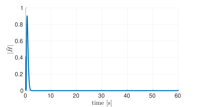
Figure 1: Time evolution of the robot’s momentum error when standing on one foot and when the control law (20a) is applied. Simulation run with the custom environment.

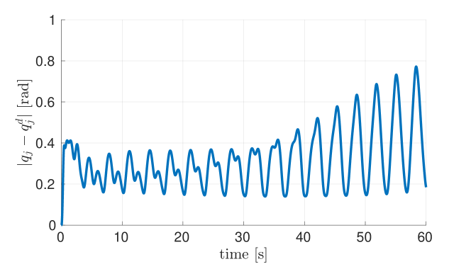
Figure 2: Time evolution of the norm of the position error $|q_{j}-q^{d}_{j}|$ when the robot is standing on one foot and when the control law (20a) is applied. Simulation run with the custom environment.

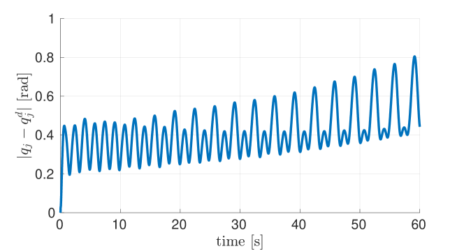
Figure 3: Time evolution of the norm of the position error $|q_{j}-q^{d}_{j}|$ when the robot is standing on two feet and when the control law (29a)- (30) is applied. Simulation run with the Gazebo environment.

IV CONTROL DESIGN

To circumvent the problems related to the stability of the zero dynamics discussed in the previous section, we propose a modification of the control laws (20a) that allows us to show stable zero dynamics of the constrained, closed loop system. The following results exploit the so-called centroidal-momentum-matrix $J_{G}(q)\in\mathbb{R}^{6\times n+6}$, namely the mapping between the robot velocity $\nu$ and the robot’s momentum $H$: $H=J_{G}(q)\nu.$ Now, observe that thanks to the results of Lemma 1 one has ${J}_{G}(q)=\begin{bmatrix}M_{b}&0_{6\times n}\end{bmatrix}$. Then, observe that when Assumption 1 is satisfied, Eq. (12) allows us to write the robot’s momentum linearly w.r.t. the robot’s joint velocity, i.e. $H=\bar{J}_{G}(q_{j})\dot{q}_{j},$ where $\bar{J}_{G}(q_{j})\in\mathbb{R}^{6\times n}$ is: ˇ

$$\bar{J}_{G}(q_{j}) \mathrel{\mathop{\mathchar 58\relax}}= \begin{bmatrix}{J}_{G}^{L}(q_{j})\\ {J}_{G}^{\omega}(q_{j})\end{bmatrix}=-M_{b}J^{-1}_{b}J_{j},$$ (31)

and ${J}_{G}^{L}(q_{j}),{J}_{G}^{\omega}(q_{j})\in\mathbb{R}^{3\times n}$. In light of the above, the following result holds.

Lemma 2.

Assume that Assumption 1 holds, and that the robot possesses more than six degrees of freedom, i.e. $n\geq 6$. In addition, assume also that $H_{d}=0$. Let

$$(q_{j},\dot{q}_{j}) = (q^{d}_{j},0)$$ (32)

denote the equilibrium point associated with the constrained, closed loop system and assume that the matrix $\Lambda=J_{j}(q)M^{-1}_{j}(q)$ is full row rank in a neighborhood of (32). Apply the control laws (20a) with

$$\dot{I}_{\tilde{H}} = \begin{bmatrix}{J}_{G}^{L}(q_{j})\\ {J}_{G}^{\omega}(q^{d}_{j})\end{bmatrix}\dot{q}_{j}$$ (33)

$$K_{i} > 0,\quad K^{j}_{p}=\hbox to0.0pt{\hskip 2.10416pt\leavevmode\hbox{$\overline{\hbox{}}$}\hss}{\leavevmode\hbox{$K$}}^{j}_{p}N_{\Lambda}M_{j},\quad K^{j}_{d}=\hbox to0.0pt{\hskip 2.10416pt\leavevmode\hbox{$\overline{\hbox{}}$}\hss}{\leavevmode\hbox{$K$}}^{j}_{d}N_{\Lambda}M_{j},$$ (34)

where $\hbox to0.0pt{\hskip 2.10416pt\leavevmode\hbox{$\overline{\hbox{}}$}\hss}{\leavevmode\hbox{$K$}}^{j}_{p},\hbox to0.0pt{\hskip 2.10416pt\leavevmode\hbox{$\overline{\hbox{}}$}\hss}{\leavevmode\hbox{$K$}}^{j}_{d}\in\mathbb{R}^{n\times n}$ are two constant, positive definite matrices. Then, the equilibrium point (32) of the constrained, closed loop dynamics is asymptotically stable.

The proof is in Appendix. Lemma 2 shows that the asymptotic stability of the equilibrium point (32) of the constrained, closed loop dynamics can be ensured by modifying the integral correction terms, and by modifying the gains of the postural task. As a consequence, the asymptotic stability of the equilibrium point (32) implies that the zero dynamics are locally asymptotically stable.

The fact that the gain matrix $K_{i}$ must be positive definite conveys the necessity of closing the control loop with orientation terms at the angular momentum level. In fact, some authors intuitively close the angular momentum loop by using the orientation of the robot’s torso [7].

The proof of Lemma 2 exploits the fact that the minimum coordinates of the robot configuration space when Assumption 1 holds is given by the joint angles $q_{j}$. The analysis focuses on the closed loop dynamics of the form $\ddot{q}_{j}=f({q}_{j},\dot{q}_{j})$ which is then linearized around the equilibrium point (32). By means of a Lyapunov analysis, one shows that the equilibrium point is asymptotically stable. One of the main technical difficulties when linearizing the equation $\ddot{q}_{j}=f({q}_{j},\dot{q}_{j})$ comes from the fact that the closed loop dynamics depends on the integral of the robot momentum, i.e.

$${I}_{\tilde{H}}(t) = {I}_{\tilde{H}}(0)+\int_{0}^{t}\begin{bmatrix}{J}_{G}^{L}(q_{j}(s))\\ {J}_{G}^{\omega}(q^{d}_{j})\end{bmatrix}\dot{q}_{j}(s)\operatorname{d\!}s$$ (35)

The partial derivative of ${I}_{\tilde{H}}(t)$ w.r.t. the state $(q_{j},\dot{q}_{j})$ is, in general, not obvious because the matrix ${J}_{G}^{L}(q_{j})$ may not be integrable. Let us observe, however, that the first three rows of $\dot{I}_{\tilde{H}}(t)$ correspond to the velocity of the center-of-mass times the robot’s mass when expressed in terms of the minimal coordinates $q_{j}$, i.e. ${J}_{G}^{L}(q_{j})\dot{q}_{j}=m\dot{x}_{c}$, with $\dot{x}_{c}\in\mathbb{R}^{3}$ the velocity of the robot’s center-of-mass. Clearly, this means that ${J}_{G}^{L}(q_{j})$ is integrable, and that

$$\partial_{q_{j}}{I}_{\tilde{H}} = \begin{bmatrix}{J}_{G}^{L}(q_{j})\\ {J}_{G}^{\omega}(q^{d}_{j})\end{bmatrix}\quad\quad\partial_{\dot{q}_{j}}{I}_{\tilde{H}}=0$$ (36)

Remark 2.

Lemma 2 suggests that applying the control laws (20a) with the control gains as (34) can still guarantee stability and convergence of the equilibrium point. First, observe that the main difference between the variable $I_{\tilde{H}}$ governed by the two expressions (16a) and (33) resides only in the last three equations. Then, more importantly, note that the momentum $H$ when Assumption 1 holds can be expressed as follows $H=\bar{J}_{G}(q_{j}^{d})\dot{q}_{j}+\emph{o}(q_{j}-q^{d}_{j},\dot{q}_{j})$ which implies that

$$\int_{0}^{t}H\operatorname{d\!}s = \bar{J}_{G}(q_{j}^{d})(q_{j}-{q}_{j}^{d})+\int_{0}^{t}\emph{o}(q_{j}-q^{d}_{j},\dot{q}_{j})\operatorname{d\!}s$$

As a consequence, the linear approximations of the integrals $I_{\tilde{H}}$ governed by (16a) and (33) coincide when

$$\lim_{(q_{j}{-}q^{d}_{j},\dot{q}_{j})\to 0}\frac{|\int_{0}^{t}\emph{o}(q_{j}-q^{d}_{j},\dot{q}_{j})\operatorname{d\!}s|}{|(q_{j}{-}q^{d}_{j},\dot{q}_{j})|}=0$$ (37)

Under the above assumption (37), the linear approximation of the control laws (20a) when evaluated with (16a) and (33) coincide, and stability and convergence of the equilibrium point $(q^{d}_{j},0)$ can still be proven.

V SIMULATIONS AND EXPERIMENTAL RESULTS

This section shows simulation and experimental results obtained by applying the control laws (20a)-(34) and (29a)-(30)-(34). To show the improvements of the control modification in Lemma 2, we apply the same reference signal of Section III, which revealed unstable zero dynamics. Hence, the desired linear momentum is chosen so as to follow a sinusoidal reference on the center of mass. Also, control gains are kept equal to those used for the simulations presented in Section III.

V-A Simulation results

Figures 5 – 5 show the norm of the joint errors $|q_{j}-q^{d}_{j}|$ when the robot stands on either one or two feet, respectively. Experiments on two feet have been performed to verify the robustness of the new control architecture. The simulations are performed both with the custom and Gazebo environment. As expected, the zero dynamics is now stable, and no divergent behavior of the robot joints is observed.

V-B Results on the iCub Humanoid Robot

We then went one step further and implemented the control algorithm  (29a)-(30) with the modification presented in Lemma 2 on the real humanoid robot. The robotic platform used for testing is the iCub humanoid robot [28]. For the purpose of the proposed control law, iCub is endowed with $23$ degrees of freedom. A low level torque control loop, running at $1\mathrm{kHz}$, is responsible for stabilizing any desired torque reference signal.

Figures 7 – 7 show the joint position error $|q_{j}-q^{d}_{j}|$ and the center of mass error. Though the center of mass does not converge to the desired value, all signals are bounded, and the control modification presented in Lemma 2 does not pose any barrier for the implementation of the control algorithm (29a)- (30) on a real platform.

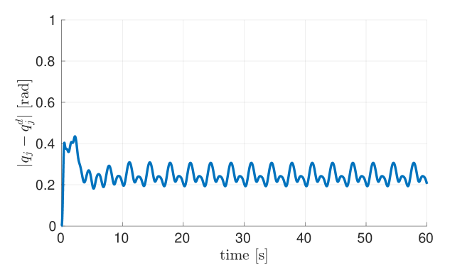
Figure 4: Time evolution of the norm of the position error $|q_{j}-q^{d}_{j}|$ when the robot is standing on one foot and when the control law (20a)–(34)–(33) is applied. Simulation run with the custom environment.

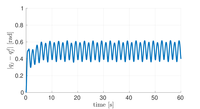
Figure 5: Time evolution of the norm of the position error $|q_{j}-q^{d}_{j}|$ when the robot is standing on two feet and when the control law (29a)–(30)–(34)–(33) is applied. Simulation run with the Gazebo environment.

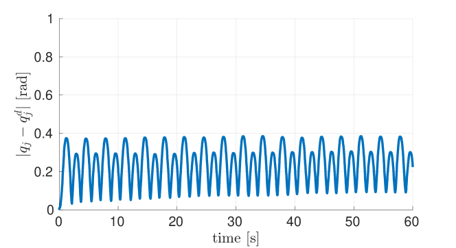
Figure 6: Time evolution of the position error norm $|q_{j}-q^{d}_{j}|$ when the robot is standing on two feet and when the laws (29a)–(30)–(34)–(33) are applied. Experiment run on the humanoid robot iCub.

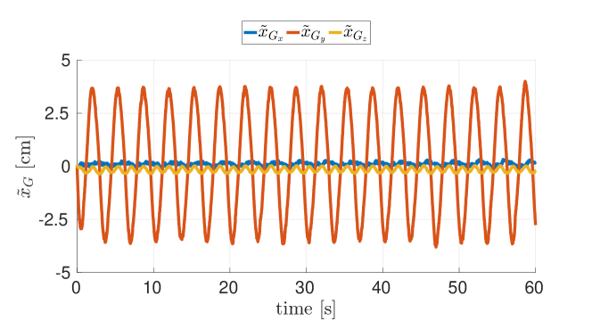
Figure 7: Time evolution of robot center-of-mass errors $\tilde{x}_{G}$ when the robot stands on two feet and when the laws (29a)–(30)–(34)–(33) are applied. Experiment run on the humanoid robot iCub.

VI CONCLUSIONS AND FUTURE WORKS

Momentum-based controllers are an efficient control strategy for performing balancing and walking tasks on humanoids. In this paper, we presented numerical evidence that a stack-of-task approach to this kind of controllers may lead to an instability of the zero dynamics. In particular, to ensure stability, it is necessary to close the loop with orientation terms at the momentum level. We show a modification of state-of-the-art momentum based control strategies that ensure asymptotic stability, which was shown by performing Lyapunov analysis on the linearization of the closed loop system around the equilibrium point. Simulation and experimental tests validate the presented analysis.

The stack-of-task approach strongly resembles a cascade of dynamical systems. It is the authors’ opinion that the stability of the whole system can be proved by using the general framework of stability of interconnected systems. A critical point needed to prove the stability of constrained dynamical system is to define the minimum set of coordinates identifying its evolution. This can be straightforward in case of one contact, but the extension to multiple contacts is not trivial and must be considered carefully.

APPENDIX: proof of Lemma 2

As described in Section IV the proof is composed of two steps. First, we linearize the constrained closed loop dynamics around the equilibrium $(q_{j}^{d},0)$. Then, by means of Lyapunov analysis, we show that the equilibrium point is asymptotically stable.

VI-1 Linearization

Consider that Assumption 1 holds, and that we apply the control laws (20a)-(33) with the gains as (34). The closed loop joint space dynamics of system (6) constrained by (13) is given by the following equation:

$$M_{j}\ddot{q}_{j}+h_{j}-J_{j}^{\top}f=\tau$$ (38)

Now, rewrite (20a) as follows: $\tau=\Lambda^{+}(\Lambda(h_{j}-J_{j}^{\top}f)+J_{b}M_{b}^{-1}(h_{b}-J_{b}^{\top}f)-\dot{J}\nu)+N_{\Lambda}\tau_{0}$. Therefore, Eq. (38) can be simplified into:

$$\ddot{q}_{j}=M_{j}^{-1}(\Lambda^{+}(J_{b}M_{b}^{-1}(h_{b}-J_{b}^{\top}f)-\dot{J}\nu)-N_{\Lambda}u_{0})$$ (39)

where $u_{0}=K^{j}_{p}(q_{j}-q_{j}^{d})+K^{j}_{d}\dot{q}_{j}$, while $h_{b}=C_{b}\nu_{b}+C_{bj}\dot{q}_{j}+mge_{3}$, and $C_{b}\in\mathbb{R}^{6\times 6}$, $C_{bj}\in\ \mathbb{R}^{6\times n}$, $C_{jb}\in\ \mathbb{R}^{n\times 6}$, $C_{j}\in\ \mathbb{R}^{n\times n}$ are obtained from the following partition of the Coriolis matrix:

$$C = \begin{bmatrix}C_{b}&C_{bj}\\ C_{jb}&C_{j}\end{bmatrix}$$

Substituting (18) into (39) and grouping together the terms that are linear with respect of joint velocity yield:

$$\ddot{q}_{j}=-M_{j}^{-1}\left[\Lambda^{\dagger}(J_{b}M_{b}^{-1}\dot{H}^{*}+\Gamma\dot{q}_{j})+N_{\Lambda}u_{0}\right]$$ (40)

where $\Gamma=\dot{J}_{j}-J_{b}M_{b}^{-1}C_{bj}+(J_{b}M_{b}^{-1}C_{b}-\dot{J}_{b})J_{b}^{-1}J_{j}$.
Define the state $x$ as $x\mathrel{\mathop{\mathchar 58\relax}}=\begin{bmatrix}x_{1}^{\top}&x_{2}^{\top}\end{bmatrix}^{\top}=\begin{bmatrix}q_{j}^{\top}-q^{d\top}_{j}&\dot{q}_{j}^{\top}\end{bmatrix}^{\top}.$ Since $H^{d}\equiv 0$, the linearized dynamical system about the equilibrium point $(q_{j}^{d},0)$ is given by

$$\dot{x}=\begin{bmatrix}\partial_{q_{j}}\dot{x}_{1}&\partial_{\dot{q}_{j}}\dot{x}_{1}\\ \partial_{q_{j}}\dot{x}_{2}&\partial_{\dot{q}_{j}}\dot{x}_{2}\end{bmatrix}x=\begin{bmatrix}0_{n\times n}&1_{n}\\ A_{1}&A_{2}\end{bmatrix}x$$ (41)

To find the matrices $A_{1},A_{2}\in\mathbb{R}^{n\times n}$, one has to evaluate the following partial derivatives

$$\partial_{y}\ddot{q}_{j} = -\sum_{i=1}^{6}\partial_{y}(M_{j}^{-1}\Lambda^{\dagger}J_{b}M_{b}^{-1}e_{i})e_{i}^{\top}\dot{H}^{*}-M_{j}^{-1}N_{\Lambda}\partial_{y}u_{0}$$

$$-\sum_{i=1}^{n}\partial_{y}(M_{j}^{-1}N_{\Lambda}e_{i})e_{i}^{\top}u_{0}-M_{j}^{-1}\Lambda^{\dagger}J_{b}M_{b}^{-1}\partial_{y}\dot{H}^{*}$$

with $y=\{q_{j},\dot{q}_{j}\}$. Note that $\dot{H}^{*}=0$ and $u_{0}=0$ when evaluated at $q_{j}=q_{j}^{d}$ and $\dot{q}_{j}=0$. We thus have to compute only the partial derivatives of $\dot{H}^{*}$ and $u_{0}$. The latter is trivially given by $\partial_{q_{j}}u_{0}=\hbox to0.0pt{\hskip 2.10416pt\leavevmode\hbox{$\overline{\hbox{}}$}\hss}{\leavevmode\hbox{$K$}}^{j}_{p}N_{\Lambda}M_{j}$ and $\partial_{\dot{q}_{j}}u_{0}=\hbox to0.0pt{\hskip 2.10416pt\leavevmode\hbox{$\overline{\hbox{}}$}\hss}{\leavevmode\hbox{$K$}}^{j}_{d}N_{\Lambda}M_{j}$. The former can be calculated via Eq. (36). In light of the above we obtain the expressions of the matrices in (41):

$$A_{1} = -M_{j}^{-1}\Lambda^{\dagger}J_{b}M_{b}^{-1}K_{i}M_{b}J_{b}^{-1}J_{j}-M_{j}^{-1}N_{\Lambda}\hbox to0.0pt{\hskip 2.10416pt\leavevmode\hbox{$\overline{\hbox{}}$}\hss}{\leavevmode\hbox{$K$}}^{j}_{p}N_{\Lambda}M_{j}$$

$$A_{2} = -M_{j}^{-1}\Lambda^{\dagger}J_{b}M_{b}^{-1}K_{p}M_{b}J_{b}^{-1}J_{j}-M_{j}^{-1}N_{\Lambda}\hbox to0.0pt{\hskip 2.10416pt\leavevmode\hbox{$\overline{\hbox{}}$}\hss}{\leavevmode\hbox{$K$}}^{j}_{d}N_{\Lambda}M_{j}.$$

VI-2 Proof of Asymptotic Stability

Consider now the following Lyapunov candidate:

$$V(x) {=} \frac{1}{2}\left[{x}_{1}^{\top}M_{j}^{\top}Q_{1}M_{j}{x}_{1}{+}x_{2}^{\top}M_{j}^{\top}Q_{2}M_{j}x_{2}\right]$$

where $M_{j}=M_{j}(q_{j}^{d})$, and

$$Q_{1} \mathrel{\mathop{\mathchar 58\relax}}=\Lambda^{\top}J_{b}^{-\top}M_{b}^{\top}K_{i}M_{b}J_{b}^{-1}\Lambda+N_{\Lambda}\hbox to0.0pt{\hskip 2.10416pt\leavevmode\hbox{$\overline{\hbox{}}$}\hss}{\leavevmode\hbox{$K$}}_{p}^{j}N_{\Lambda}$$

$$Q_{2} \mathrel{\mathop{\mathchar 58\relax}}=\Lambda^{\top}J_{b}^{-\top}M_{b}^{\top}M_{b}J_{b}^{-1}\Lambda+N_{\Lambda}$$

calculated at ${x}_{1}=0$, $x_{2}=0$. $V$ is a properly defined candidate, in fact $V=0\iff x=0$ and is positive definite otherwise. Indeed, $Q_{1}$ can be rewritten in the following way:

$$Q_{1}= \begin{bmatrix}\Lambda^{\top}&N_{\Lambda}\end{bmatrix}\begin{bmatrix}J_{b}^{-\top}M_{b}^{\top}K_{i}M_{b}J_{b}^{-1}&0\\ 0&\hbox to0.0pt{\hskip 2.10416pt\leavevmode\hbox{$\overline{\hbox{}}$}\hss}{\leavevmode\hbox{$K$}}_{p}^{j}\end{bmatrix}\begin{bmatrix}\Lambda\\ N_{\Lambda}\end{bmatrix}.$$

and, because $\Lambda$ and $N_{\Lambda}$ are orthogonal $Q_{1}$ is positive definite. The same reasoning can be applied to $Q_{2}$.

We can now consider the time derivative of $V$:

$$\dot{V} = {x}_{1}^{\top}M_{j}^{\top}Q_{1}M_{j}x_{2}+x_{2}^{\top}M_{j}^{\top}Q_{2}M_{j}\dot{x}_{2}$$

$$= -x_{2}^{\top}M_{j}^{\top}(\Lambda^{\top}J_{b}^{-\top}M_{b}^{\top}K_{p}M_{b}J_{b}^{-1}\Lambda$$

$$+N_{\Lambda}K^{j}_{d}N_{\Lambda})M_{j}x_{2}\leq 0.$$

The stability of the equilibrium point $x=0$ associated with the linear system (41) thus follows. To prove the asymptotic stability of the equilibrium point $x=0$, which implies its asymptotic stability when associated with the nonlinear system (40), we have to resort to LaSalle’s invariance principle. Let us define the invariant set $S\mathrel{\mathop{\mathchar 58\relax}}=\{x\mathrel{\mathop{\mathchar 58\relax}}\dot{V}(x)=0\}$ that implies $S=\{({x}_{1},0)\}$. It is easy to verify that the only trajectory starting in $S$ and remains in $S$ is given by ${x}_{1}=0$ thus proving LaSalle’s principle. As a consequence, the equilibrium point $x=0\Rightarrow(q_{j},\dot{q}_{j})=(q_{j}^{d},0)$ is asymptotically stable.

References

- [1] S. Caux, E. Mateo, and R. Zapata, “Balance of biped robots: special double-inverted pendulum,” Systems, Man, and Cybernetics, 1998. 1998 IEEE International Conference on, 1998.
- [2] K. Hirai, M. Hirose, Y. Haikawa, and T. Takenaka, “The development of Honda humanoid robot,” Robotics and Automation, 1998. Proceedings. 1998 IEEE International Conference on, 1998.
- [3] S. Hyon, J. Hale, and G. Cheng, “Full-body compliant human-humanoid interaction: Balancing in the presence of unknown external forces,” Robotics, IEEE Transactions on, Oct 2007.
- [4] Q. Huang, K. Kaneko, K. Yokoi, S. Kajita, T. Kotoku, N. Koyachi, H. Arai, N. Imamura, K. Komoriya, and K. Tanie, “Balance control of a biped robot combining off-line pattern with real-time modification,” Robotics and Automation, 2000. Proceedings. ICRA ’00. IEEE International Conference on, 2000.
- [5] R. Featherstone, Rigid Body Dynamics Algorithms. Secaucus, NJ, USA: Springer-Verlag New York, Inc., 2007.
- [6] J. A. Acosta and M. Lopez-Martinez, “Constructive feedback linearization of underactuated mechanical systems with 2-DOF,” Decision and Control, 2005 and 2005 European Control Conference. CDC-ECC ’05. 44th IEEE Conference on, 2005.
- [7] C. Ott, M. Roa, and G. Hirzinger, “Posture and balance control for biped robots based on contact force optimization,” in Humanoid Robots (Humanoids), 2011 11th IEEE-RAS International Conference on, Oct 2011, pp. 26–33.
- [8] P. Wensing and D. Orin, “Generation of dynamic humanoid behaviors through task-space control with conic optimization,” in Robotics and Automation (ICRA), 2013 IEEE International Conference on, May 2013, pp. 3103–3109.
- [9] F. Nori, S. Traversaro, J. Eljaik, F. Romano, A. Del Prete, and D. Pucci, “iCub whole-body control through force regulation on rigid noncoplanar contacts,” Frontiers in Robotics and AI, vol. 2, no. 6, 2015.
- [10] B. Stephens and C. Atkeson, “Dynamic balance force control for compliant humanoid robots,” in Intelligent Robots and Systems (IROS), 2010 IEEE/RSJ International Conference on, Oct 2010, pp. 1248–1255.
- [11] A. Herzog, L. Righetti, F. Grimminger, P. Pastor, and S. Schaal, “Balancing experiments on a torque-controlled humanoid with hierarchical inverse dynamics,” in Intelligent Robots and Systems (IROS 2014), 2014 IEEE/RSJ International Conference on, Sept 2014, pp. 981–988.
- [12] T. Koolen, S. Bertrand, G. Thomas, T. de Boer, T. Wu, J. Smith, J. Englsberger, and J. Pratt, “Design of a momentum-based control framework and application to the humanoid robot atlas,” International Journal of Humanoid Robotics, vol. 13, p. 34, March 2016.
- [13] L. Righetti, J. Buchli, M. Mistry, and S. Schaal, “Inverse dynamics control of floating-base robots with external constraints: A unified view,” IEEE International Conference on Robotics and Automation, May 2011.
- [14] ——, “Control of legged robots with optimal distribution of contact forces,” in Humanoid Robots (Humanoids), 2011 11th IEEE-RAS International Conference on, Oct 2011, pp. 318–324.
- [15] J. Nakanish, M. Mistry, and S. Schaal, “Inverse Dynamics Control with Floating Base and Constraints,” Robotics and Automation, 2007 IEEE International Conference on, pp. 1942 – 1947, 2007.
- [16] M. Hopkins, R. Griffin, A. Leonessa, B. Lattimer, and T. Furukawa, “Design of a compliant bipedal walking controller for the darpa robotics challenge,” in Humanoid Robots (Humanoids), 2015 IEEE-RAS 15th International Conference on, Nov 2015, pp. 831–837.
- [17] P.-B. Wieber, Holonomy and Nonholonomy in the Dynamics of Articulated Motion. Berlin, Heidelberg: Springer Berlin Heidelberg, 2006, pp. 411–425. [Online]. Available: http://dx.doi.org/10.1007/978-3-540-36119-0˙20
- [18] M. Liu and V. Padois, “Reactive whole-body control for humanoid balancing on non-rigid unilateral contacts,” Intelligent Robots and Systems (IROS), 2015 IEEE/RSJ International Conference on, pp. 3981 – 3987, 2015.
- [19] A. Hofmann, M. Popovic, and H. Herr, “Exploiting angular momentum to enhance bipedal center-of-mass control,” Robotics and Automation. ICRA ’09. IEEE International Conference on. 2009, 2009.
- [20] H. Herr and M. Popovic, “Angular momentum in human walking,” Journal of Experimental Biology, vol. 211, no. 4, pp. 467–481, 2008.
- [21] J. E. Marsden and T. S. Ratiu, Introduction to Mechanics and Symmetry: A Basic Exposition of Classical Mechanical Systems. Springer Publishing Company, Incorporated, 2010.
- [22] S. Traversaro, D. Pucci, and F. Nori, “On the base frame choice in free-floating mechanical systems and its connection to “centroidal” dynamics,” Submitted to Humanoid Robots (Humanoids), 2016 IEEE-RAS International Conference on, 2016. [Online]. Available: https://traversaro.github.io/preprints/changebase.pdf
- [23] J. E. Marsden and J. Scheurle, “The reduced euler-lagrange equations,” Fields Institute Comm, vol. 1, pp. 139–164, 1993.
- [24] J. Jellinek and D. Li, “Separation of the energy of overall rotation in any n-body system,” Physical review letters, vol. 62, no. 3, p. 241, 1989.
- [25] H. Essén, “Average angular velocity,” European journal of physics, vol. 14, no. 5, p. 201, 1993.
- [26] D. Orin, A. Goswami, and S.-H. Lee, “Centroidal dynamics of a humanoid robot,” Autonomous Robots, 2013.
- [27] S.-H. Lee and A. Goswami, “Ground reaction force control at each foot: A momentum-based humanoid balance controller for non-level and non-stationary ground,” in Intelligent Robots and Systems (IROS), 2010 IEEE/RSJ International Conference on, Oct 2010, pp. 3157–3162.
- [28] G. Metta, L. Natale, F. Nori, G. Sandini, D. Vernon, L. Fadiga, C. von Hofsten, K. Rosander, M. Lopes, J. Santos-Victor, A. Bernardino, and L. Montesano, “The iCub humanoid robot: An open-systems platform for research in cognitive development,” Neural Networks, vol. 23, no. 8–9, pp. 1125 – 1134, 2010, social Cognition: From Babies to Robots.
- [29] S. Gros, M. Zanon, and M. Diehl, “Baumgarte stabilisation over the SO(3) rotation group for control,” 2015 54th IEEE Conference on Decision and Control (CDC), pp. 620–625, December 2015.
- [30] N. Koenig and A. Howard, “Design and use paradigms for gazebo, an open-source multi-robot simulator,” Intelligent Robots and Systems, 2004. (IROS 2004). Proceedings. 2004 IEEE/RSJ International Conference on, pp. 2149 – 2154, 2004.