Quark ACM with topologically generated gluon mass

Abstract

We investigate the effect of a small, gauge-invariant mass of the gluon on the anomalous chromomagnetic moment of quarks (ACM) by perturbative calculations at one loop level. The mass of the gluon is taken to have been generated via a topological mass generation mechanism, in which the gluon acquires a mass through its interaction with an antisymmetric tensor field $B_{\mu\nu}$. For a small gluon mass $(<10$ MeV), we calculate the ACM at momentum transfer $q^{2}=-M_{Z}^{2}$. We compare those with the ACM calculated for the gluon mass arising from a Proca mass term. We find that the ACM of up, down, strange and charm quarks vary significantly with the gluon mass, while the ACM of top and bottom quarks show negligible gluon mass dependence. The mechanism of gluon mass generation is most important for the strange quarks ACM, but not so much for the other quarks. We also show the results at $q^{2}=-m_{t}^{2}$. We find that the dependence on gluon mass at $q^{2}=-m_{t}^{2}$ is much less than at $q^{2}=-M_{Z}^{2}$ for all quarks.

I Introduction

The anomalous chromomagnetic moment (ACM) of quarks does not yet have a precise experimental bound. As the Large Hadron Collider (LHC) climbs new peaks of luminosity and energy, it opens new windows on precision QCD Bernreuther:2015yna , which should allow investigations into the anomalous couplings such as the ACM Franzosi:2015osa .

The ACM of light quarks can be calculated in nonperturbative QCD Kochelev:1996pv ; Kochelev:2013zoa ; Kochelev:2013csa ; Chang:2010hb . However, perturbative calculations of this quantity has received little attention so far, mainly because perturbative calculations in QCD do not make sense at very low energies. Since the QCD coupling constant diminishes rapidly with increasing energy, precision measurements are needed to measure the ACM at large momentum transfer. Although some bounds on top quark ACM have been provided by early theoretical analyses using a general effective Lagrangian with an anomalous coupling Rindani:2015vya ; Martinez:1996cy ; Martinez:2001qs ; Martinez:2007qf ; Gaitan:2015aia ; Hioki:2009hm ; Hioki:2010zu ; Kamenik:2011dk ; Biswal:2012dr ; Choudhury:2012np ; Labun:2012ra ; Degrande:2012gr ; Ayazi:2013cba ; Hioki:2013hva ; Hesari:2014hva , the only experimental analysis so far was done by the CMS collaboration last year CMS:2014bea .

Another quantity not known very precisely, thus requiring more investigation, is the mass of the gluon. Gluons are taken to be massless in QCD essentially because color symmetry is unbroken as far as we know – there is no spontaneous symmetry breaking in QCD. However, thus far experiments have failed to find a stringent bound on the mass of the gluon Beringer:1900zz . Theoretical analyses regarding gluon mass have provided us with estimates varying over a large range, from a few MeV to several hundred MeV Cornwall:1981zr ; Aguilar:2009ke ; Parisi:1980jy ; Field:2001iu ; Yndurain:1995uq ; Nussinov:2010jg . However, if gluons are indeed massive particles, all gluons must have the same mass, since one gluon cannot be distinguished from another if the SU(3) global symmetry is unbroken. There are different ways for a gluon to be massive without symmetry breaking Cornwall:1981zr ; Curci:1976bt ; deBoer:1995dh , the topological mass generation mechanism Allen:1991gb ; Hwang:1995er ; Lahiri:1996dm ; Lahiri:2001uc is one of them.

In a previous paper Choudhury:2014lna , a small Proca mass was considered for the gluon, so that all gluons had the same mass, and the anomalous chromomagnetic moment of each quark was calculated perturbatively. However, those results can be relevant only if the gluon is massive either via the Proca model, which is known to be unitary but non-renormalizable Curci:1976bt ; deBoer:1995dh , or gets a dynamically generated mass, in which case the mass is likely to go to zero at higher energies Cornwall:1981zr where perturbation calculations make any sense. The other possibility is to use the topological mass mechanism, which does not break the symmetry, thus giving the same mass to all gluons, and may have the additional virtue of being unitary and renormalizable Hwang:1995er ; Lahiri:1996dm ; Lahiri:2001uc . In this paper we present a perturbative calculation of the anomalous chromomagnetic moment of quarks, assuming a small, topologically generated, gauge-invariant mass for the gluon.

The quark-gluon interaction term which corresponds to the anomalous chromomagnetic moment is given by

$$ig\bar{\psi}\sigma_{\mu\nu}T^{a}\psi\,F_{2}(q^{2})q^{\nu}G^{\mu a}\,.$$ (1)

The coefficient $F_{2}(q^{2})$ is the ACM of the quark at momentum transfer $q$. We will calculate this term in perturbation theory at one loop, assuming a small mass for the gluon. Since QCD is a strongly coupled theory at low energies, the ACM cannot be calculated perturbatively for $q^{2}=0$, but only at sufficiently large momentum transfer. We will give numerical results for $q^{2}=-M_{Z}^{2}$ as well as for $q^{2}=-m_{t}^{2}$ .

As mentioned above, a topological mass generation mechanism will be taken to be responsible for the mass of the gluon. This mechanism involves an antisymmetric tensor field $B_{\mu\nu}$ coupled to the field strength $F_{\mu\nu}$ of the gluon field through a $B\wedge F$ coupling. A Lagrangian which implements this is

$${\cal L}=-\frac{1}{4}F_{\mu\nu}^{a}F^{a\mu\nu}+\frac{1}{12}H^{a}_{\mu\nu\lambda}H^{a\mu\nu\lambda}+\frac{M}{4}\epsilon^{\mu\nu\rho\lambda}F^{a}_{\mu\nu}B^{a}_{\rho\lambda}\,,$$ (2)

where $F_{\mu\nu}$ is the field strength tensor of the gluon field $G_{\mu}$, and $H_{\mu\nu\lambda}=D_{[\mu}B_{\nu\lambda]}$ is the field strength of the antisymmetric tensor field $B^{a}_{\mu\nu}$. The gluon mass $M$ is a free parameter of the theory.

This Lagrangian is invariant under local $SU(3)$ gauge transformations

$$G_{\mu} \rightarrow UG_{\mu}U^{-1}-\frac{i}{g}\partial_{\mu}UU^{-1},$$ (3)

$$B_{\mu\nu} \rightarrow UB_{\mu\nu}U^{-1}\,.$$ (4)

For the quantization of the gauge fields we add two gauge fixing terms,

$${\cal L}_{GF}=-\frac{1}{2\xi}(\partial_{\mu}G^{\mu}_{a})^{2}-\frac{1}{2\eta}(D_{\mu}B^{\mu\nu}_{a})^{2}\,.$$ (5)

While the first of these two terms fixes the gauge for SU(3) transformations, the role of the second term is somewhat more complicated. There is a higher gauge transformation for the $B$ field, under $B_{\mu\nu}\to B_{\mu\nu}+D_{[\mu}\Lambda_{\nu]}$ , which can be implemented in the Lagrangian by use of an auxiliary field Hwang:1995er ; Lahiri:1996dm ; Lahiri:2001uc . This additional gauge transformation is fixed by the second term. We have not shown the auxiliary field because its couplings do not appear in the one-loop diagrams responsible for the ACM.

The propagators of the gluon and the tensor field $B_{\mu\nu}$ can now be calculated. Ignoring the mixed quadratic term for the moment, we find the propagators

$$i\Delta^{\mu\nu,ab} =-\frac{i}{k^{2}}\left(g^{\mu\nu}-(1-\xi)\dfrac{k^{\mu}k^{\nu}}{k^{2}}\right)\delta^{ab},$$ (6)

$$i\Delta^{\mu\nu,\rho\lambda;ab} =\frac{i}{k^{2}}\left(g^{\mu[\rho}g^{\lambda]\nu}-(1-\eta)\dfrac{k^{\mu}k^{[\lambda}g^{\rho]\nu}-k^{\nu}k^{[\lambda}g^{\rho]\mu}}{k^{2}}\right)\delta^{ab}\,.$$ (7)

The $BF$ interaction term contains a quadratic derivative interaction between the two fields, as well as a cubic interaction. The vertices for these interactions are shown in Fig. 1 and Fig. 1. The vertex rule corresponding to the 2-point vertex diagram is

$$iV^{ab}_{\mu\nu,\lambda}=-M\epsilon_{\mu\nu\lambda\rho}k^{\rho}\delta^{ab}\,.$$ (8)

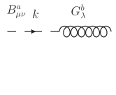
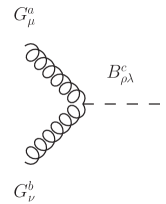
Figure 1: (a) The two-point $G-B$ vertex ; (b) the cubic $G-G-B$ vertex

The 2-point vertex corresponds to an off-diagonal mixing term between the gluon and the $B$ fields. The ‘effective’ bare propagator of the gluon field is obtained by summing over the series of gluon propagators containing all possible insertions of the $B$ propagator via the 2-point vertex, as shown in Fig. 2. The result is

$$iD_{\mu\nu}=-i\dfrac{g_{\mu\nu}-k_{\mu}k_{\nu}/k^{2}}{k^{2}-M^{2}+i\epsilon}+i\xi\dfrac{k_{\mu}k_{\nu}}{k^{4}}\,,$$ (9)

showing the presence of a pole in the propagator, corresponding to a mass $M$ . We will see below that the terms proportional to $k_{\mu}k_{\nu}$ will not contribute in the ACM calculations, as all internal gluon lines couple to a conserved current at least at one end.

Figure 2: Bare gluon propagator by summing over all possible insertions of the $B$ propagator

The three-point vertex of Fig. 1 contributes to the one-loop diagrams for the ACM. The vertex rule for this diagram is

$$iV^{ab}_{\mu,\nu,\lambda\rho}=-igMf^{bca}\epsilon_{\mu\nu\lambda\rho}\,.$$ (10)

There are two more vertices involving the $B$ field, coming from the $H^{2}$ term in the Lagrangian. These two are shown in Fig. 3 and Fig. 3, and the corresponding vertex rules are

$$iV^{abc}_{\mu,\lambda\rho,\sigma\tau}=gf^{abc}\left[(p-q)_{\mu}g_{\lambda[\sigma}g_{\tau]\rho}+\left(p+q/{\eta}\right)_{[\sigma}g_{\tau][\lambda}g_{\rho]\mu}-\left(q+p/{\eta}\right)_{[\lambda}g_{\rho][\sigma}g_{\tau]\mu}\right]\,,$$ (11)

and

$$iV^{abcd}_{\mu,\nu,\lambda\rho,\sigma\tau} = ig^{2}\left[f_{ace}f_{bde}\left(g_{\mu\nu}g_{\lambda[\sigma}g_{\tau]\rho}+g_{\mu[\sigma}g_{\tau]g[\lambda}g_{\rho]\nu}-\frac{1}{\eta}g_{\mu[\lambda}g_{\rho][\sigma}g_{\tau]\nu}\right)\right.$$ (12)

$$\qquad+\left.f_{ade}f_{bce}\left(g_{\mu\nu}g_{\lambda[\sigma}g_{\tau]\rho}+g_{\mu[\lambda}g_{\rho]g[\sigma}g_{\tau]\nu}-\frac{1}{\eta}g_{\mu[\sigma}g_{\tau]g[\lambda}g_{\rho]\nu}\right)\right].\qquad\,$$

Only the three-point vertex will contribute to the 1-loop diagrams for the ACM.

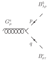
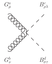
Figure 3: (a) $GBB$ vertex and (b) $GGBB$ vertex, from $\dfrac{1}{12}H^{a}_{\mu\nu\lambda}H^{a\mu\nu\lambda}$

There are of course other contributions to the ACM that we have to take into account. Let us list all the relevant 1-loop diagrams.

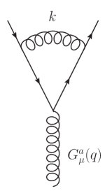
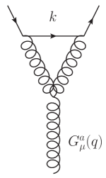
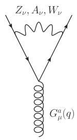
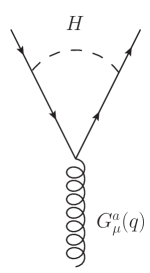
Figure 4: Strong and electroweak contributions to the ACM of a quark: strong contribution: (a) QED-like diagram; (b) purely non-Abelian contribution; weak contributions: (c) gauge boson exchange; (d) Higgs boson exchange.

The ACM of quarks receives contributions from both strong and weak processes at one loop order. Fig. 4 shows the diagrams corresponding to strong and weak contributions. The new three-point vertices coming from topological mass generation give rise to some more diagrams which contribute to the gluon ACM. These new diagrams are shown in Fig. 5.

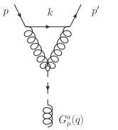
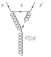
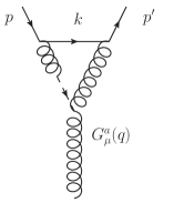
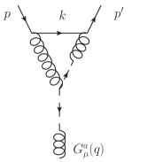
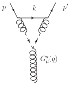
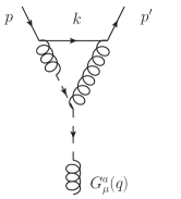
Figure 5: Topological contribution to the ACM of a quark.

Since $B$ does not couple to quarks directly, the contribution of the diagrams in Fig. 5 may be thought of as a correction to the diagram in Fig. 4. We can calculate this conveniently by first removing the quark lines from each of the diagrams in Fig. 5 and then adding together the remaining parts. The resulting effective topological three-gluon vertex can be written as

$$V^{abc}(\bar{p},\bar{q},\bar{r}) = \frac{gM^{2}f^{abc}}{\bar{p}^{2}\bar{q}^{2}\bar{r}^{2}}\left[36\bar{q}^{2}\bar{r}^{2}\left(\bar{p}_{\mu}g_{\nu\lambda}-\bar{p}_{\lambda}g_{\mu\nu}\right)+36\bar{p}^{2}\bar{q}^{2}\left(\bar{r}_{\nu}g_{\mu\lambda}-\bar{r}_{\mu}g_{\lambda\nu}\right)+36\bar{p}^{2}\bar{r}^{2}\left(\bar{q}_{\lambda}g_{\mu\nu}-\bar{q}_{\nu}g_{\lambda\mu}\right)\right.$$

$$\qquad+8\bar{q}^{2}\left[(\bar{r}-\bar{p})_{\mu}\bar{r}_{\nu}\bar{p}_{\lambda}-2\bar{p}_{\mu}\bar{r}_{\nu}\bar{r}_{\lambda}+2\bar{r}_{\mu}\bar{p}_{\nu}\bar{p}_{\lambda}+(\bar{r}\cdot\bar{p})\{(\bar{p}-\bar{r})_{\mu}g_{\lambda\nu}-2\bar{p}_{\nu}g_{\lambda\mu}+2\bar{r}_{\lambda}g_{\mu\nu}\}\right]$$

$$\qquad+8\bar{p}^{2}\left[(\bar{q}-\bar{r})_{\nu}\bar{r}_{\mu}\bar{q}_{\lambda}-2\bar{q}_{\mu}\bar{r}_{\nu}\bar{q}_{\lambda}+2\bar{r}_{\mu}\bar{q}_{\nu}\bar{r}_{\lambda}+(\bar{q}\cdot\bar{r})\{-(\bar{q}-\bar{r})_{\nu}g_{\lambda\mu}-2\bar{r}_{\lambda}g_{\mu\nu}+2\bar{q}_{\mu}g_{\lambda\nu}\}\right]$$

$$\qquad\left.+8\bar{r}^{2}\left[(\bar{p}-\bar{q})_{\lambda}\bar{p}_{\mu}\bar{q}_{\nu}-2\bar{p}_{\mu}\bar{p}_{\nu}\bar{q}_{\lambda}+2\bar{q}_{\mu}\bar{q}_{\nu}\bar{p}_{\lambda}+(\bar{p}\cdot\bar{q})\{(\bar{q}-\bar{p})_{\lambda}g_{\mu\nu}-2\bar{q}_{\mu}g_{\lambda\nu}-2\bar{p}_{\nu}g_{\lambda\mu}\}\right]\right]\,,$$

where all momenta are directed towards the vertex. This $V^{abc}$ is added to the usual three-gluon vertex, and the total is used to calculate Fig. 4.

II Calculations

We substitute $\bar{p}=p-k$ , $\bar{q}=-q$ and $\bar{r}=k-p^{\prime}$ in the total effective vertex given in Eq. (LABEL:vertex.topo), and thus calculate the total contribution of all the diagrams in Fig. 5 to the vertex function. We can write the total contribution of the ‘topological’ terms to the vertex function as

$$\Gamma_{\mu} =-36iM^{2}\alpha_{s}\pi\left[\Gamma^{(1)}_{\mu}+\Gamma^{(2)}_{\mu}+\Gamma^{(3)}_{\mu}+\frac{2}{9}\Gamma^{(4)}_{\mu}+\frac{2}{9}\Gamma^{(5)}_{\mu}+\frac{2}{9}\Gamma^{(6)}_{\mu}\right]\,.$$ (14)

The superscripts on the $\Gamma_{\mu}$ on the right hand side of Eq. (14) correspond to the successive terms on the right hand side of Eq. (LABEL:vertex.topo). Using the relation

$$T_{ji^{\prime}}^{c}T_{i^{\prime}i}^{b}f^{abc}=-\frac{i}{4}T_{ji}^{a}\,,$$ (15)

we can write the different components of this equation as

$$\Gamma^{(1)}_{\mu} =\int\dfrac{d^{4}k}{(2\pi)^{4}}\dfrac{(p-k)_{\mu}\gamma_{\lambda}(\hbox to0.0pt{\hbox to5.52084pt{\hfil/\hfil}\hss}k+m)\gamma^{\lambda}-(\hbox to0.0pt{\hbox to5.03125pt{\hfil/\hfil}\hss}p-\hbox to0.0pt{\hbox to5.52084pt{\hfil/\hfil}\hss}k)(\hbox to0.0pt{\hbox to5.52084pt{\hfil/\hfil}\hss}k+m)\gamma_{\mu}}{(k^{2}-m^{2})[(k-p)^{2}-M^{2}][(k-p^{\prime})^{2}-M^{2}](k-p)^{2}}\,,$$ (16)

$$\Gamma^{(2)}_{\mu} =\int\dfrac{d^{4}k}{(2\pi)^{4}}\dfrac{\gamma_{\mu}(\hbox to0.0pt{\hbox to5.52084pt{\hfil/\hfil}\hss}k+m)(\hbox to0.0pt{\hbox to5.52084pt{\hfil/\hfil}\hss}k-\,/\kern-6.00006pt{p^{\prime}})-\gamma_{\lambda}(\hbox to0.0pt{\hbox to5.52084pt{\hfil/\hfil}\hss}k+m)\gamma^{\lambda}(k-p^{\prime})_{\mu}}{(k^{2}-m^{2})[(k-p)^{2}-M^{2}][(k-p^{\prime})^{2}-M^{2}](k-p^{\prime})^{2}}\,,$$ (17)

$$\Gamma^{(3)}_{\mu} =\frac{1}{q^{2}}\int\dfrac{d^{4}k}{(2\pi)^{4}}\dfrac{\gamma_{\mu}(\hbox to0.0pt{\hbox to5.52084pt{\hfil/\hfil}\hss}k+m)\hbox to0.0pt{\hbox to5.00002pt{\hfil$q$\hfil}\hss}/-\hbox to0.0pt{\hbox to5.00002pt{\hfil$q$\hfil}\hss}/(\hbox to0.0pt{\hbox to5.52084pt{\hfil/\hfil}\hss}k+m)\gamma_{\mu}}{(k^{2}-m^{2})[(k-p)^{2}-M^{2}][(k-p^{\prime})^{2}-M^{2}]q^{2}}\,,$$ (18)

$$\Gamma^{(4)}_{\mu} =\int\dfrac{d^{4}k}{(2\pi)^{4}}\dfrac{1}{(k^{2}-m^{2})[(k-p)^{2}-M^{2}][(k-p^{\prime})^{2}-M^{2}](k-p)^{2}(k-p^{\prime})^{2}}$$

$$\qquad\times\left[-(\hbox to0.0pt{\hbox to5.52084pt{\hfil/\hfil}\hss}k-\hbox to0.0pt{\hbox to5.03125pt{\hfil/\hfil}\hss}p)(\hbox to0.0pt{\hbox to5.52084pt{\hfil/\hfil}\hss}k+m)(\hbox to0.0pt{\hbox to5.52084pt{\hfil/\hfil}\hss}k-\hbox to0.0pt{\hbox to6.57124pt{\hfil/\hfil}\hss}p^{\prime})(2k-p-p^{\prime})_{\mu}+2(k-p)_{\mu}(\hbox to0.0pt{\hbox to5.52084pt{\hfil/\hfil}\hss}k-\hbox to0.0pt{\hbox to6.57124pt{\hfil/\hfil}\hss}p^{\prime})(\hbox to0.0pt{\hbox to5.52084pt{\hfil/\hfil}\hss}k+m)(\hbox to0.0pt{\hbox to5.52084pt{\hfil/\hfil}\hss}k-\hbox to0.0pt{\hbox to6.57124pt{\hfil/\hfil}\hss}p^{\prime})\right.$$

$$\qquad+2(k-p^{\prime})_{\mu}(\hbox to0.0pt{\hbox to5.52084pt{\hfil/\hfil}\hss}k-\hbox to0.0pt{\hbox to5.03125pt{\hfil/\hfil}\hss}p)(\hbox to0.0pt{\hbox to5.52084pt{\hfil/\hfil}\hss}k+m)(\hbox to0.0pt{\hbox to5.52084pt{\hfil/\hfil}\hss}k-\hbox to0.0pt{\hbox to5.03125pt{\hfil/\hfil}\hss}p)-(k-p^{\prime})\cdot(k-p)\{2(\hbox to0.0pt{\hbox to5.52084pt{\hfil/\hfil}\hss}k-\hbox to0.0pt{\hbox to6.57124pt{\hfil/\hfil}\hss}p^{\prime})(\hbox to0.0pt{\hbox to5.52084pt{\hfil/\hfil}\hss}k+m)\gamma_{\mu}$$

$$\qquad\left.-\gamma_{\lambda}(\hbox to0.0pt{\hbox to5.52084pt{\hfil/\hfil}\hss}k+m)\gamma^{\lambda}(2k-p-p^{\prime})_{\mu}+2\gamma_{\mu}(\hbox to0.0pt{\hbox to5.52084pt{\hfil/\hfil}\hss}k+m)(\hbox to0.0pt{\hbox to5.52084pt{\hfil/\hfil}\hss}k-\hbox to0.0pt{\hbox to5.03125pt{\hfil/\hfil}\hss}p)\}\right]\,,$$ (19)

$$\Gamma^{(5)}_{\mu} =\frac{1}{q^{2}}\int\dfrac{d^{4}k}{(2\pi)^{4}}\dfrac{\gamma_{\lambda}(\hbox to0.0pt{\hbox to5.52084pt{\hfil/\hfil}\hss}k+m)\gamma_{\nu}g^{\nu\nu^{\prime}}g^{\lambda\lambda^{\prime}}}{(k^{2}-m^{2})[(k-p)^{2}-M^{2}][(k-p^{\prime})^{2}-M^{2}](k-p^{\prime})^{2}}$$

$$\qquad\times[q_{\lambda^{\prime}}(k-p^{\prime})_{\mu}(k+p-2p^{\prime})_{\nu^{\prime}}-2(k-p^{\prime})_{\nu^{\prime}}q_{\lambda^{\prime}}q_{\mu}-2q_{\nu^{\prime}}(k-p^{\prime})_{\lambda^{\prime}}(k-p^{\prime})_{\mu}$$

$$\qquad-q\cdot(k-p^{\prime})\{g_{\mu\lambda^{\prime}}(p+k-2p^{\prime})_{\nu^{\prime}}-2g_{\mu\nu^{\prime}}(k-p^{\prime})_{\lambda^{\prime}}-2g_{\lambda^{\prime}\nu^{\prime}}q_{\mu}\}]\,,$$ (20)

$$\Gamma^{(6)}_{\mu} =\frac{1}{q^{2}}\int\dfrac{d^{4}k}{(2\pi)^{4}}\dfrac{\gamma_{\lambda}(\hbox to0.0pt{\hbox to5.52084pt{\hfil/\hfil}\hss}k+m)\gamma_{\nu}g^{\nu\nu^{\prime}}g^{\lambda\lambda^{\prime}}}{(k^{2}-m^{2})[(k-p)^{2}-M^{2}][(k-p^{\prime})^{2}-M^{2}](k-p)^{2}}$$

$$\qquad\times[-(k-p)_{\mu}q_{\nu^{\prime}}(k-2p+p^{\prime})_{\lambda^{\prime}}-2q_{\mu}(k-p)_{\lambda^{\prime}}q_{\nu^{\prime}}-2q_{\lambda^{\prime}}(k-p)_{\nu^{\prime}}(k-p)_{\mu}$$

$$\qquad+q\cdot(k-p)\{g_{\mu\nu^{\prime}}(k+p^{\prime}-2p)_{\lambda^{\prime}}-2g_{\lambda^{\prime}\mu}(k-p)_{\nu^{\prime}}-2g_{\nu^{\prime}\lambda^{\prime}}q_{\mu}\}]\,.$$ (21)

The calculation of the contributions from these terms to the ACM are given in the Appendix. Adding Eqs. (29), (32), (44) and (45), we get

$$F^{TM}_{2}({q^{2}=-M_{Z}^{2}}) =\dfrac{M^{2}\alpha_{s}}{m^{2}\pi}\left[2\int\limits_{0}^{1}d\zeta_{1}\!\int\limits_{0}^{1-\zeta_{1}}d\zeta_{2}\int\limits_{0}^{1-\zeta_{1}-\zeta_{2}}d\zeta_{3}\,\dfrac{\zeta_{1}(\frac{9}{4}\zeta_{1}+\zeta_{3})}{\left[\zeta_{1}^{2}+\zeta_{3}(1-\zeta_{1}-\zeta_{3})\frac{M_{Z}^{2}}{m^{2}}+(\zeta_{2}+\zeta_{3})\frac{M^{2}}{m^{2}}\right]^{2}}\right.$$

$$\qquad-\int\limits_{0}^{1}d\zeta_{1}\int\limits_{0}^{1-\zeta_{1}}d\zeta_{2}\int\limits_{0}^{1-\zeta_{1}-\zeta_{2}}d\zeta_{3}\int\limits_{0}^{1-\zeta_{1}-\zeta_{2}-\zeta_{3}}d\zeta_{4}$$

$$\qquad\times\dfrac{\zeta_{1}(1-2\zeta_{1})\{\zeta_{1}^{2}+(\zeta_{2}+\zeta_{3})(1-\zeta_{1}-\zeta_{2}-\zeta_{3})\frac{M_{Z}^{2}}{m^{2}}-\zeta_{1}^{3}\frac{M_{Z}^{2}}{m^{2}}+3\zeta_{1}(\zeta_{2}+\zeta_{4})\}}{\left[\zeta_{1}^{2}+(\zeta_{2}+\zeta_{3})(1-\zeta_{1}-\zeta_{2}-\zeta_{3})\frac{M_{Z}^{2}}{m^{2}}+(\zeta_{2}+\zeta_{4})\frac{M^{2}}{m^{2}}\right]^{3}}$$

$$\qquad\left.-\frac{9M_{Z}^{2}}{2m^{2}}\int\limits_{0}^{1}d\zeta_{1}\int\limits_{0}^{1-\zeta_{1}}d\zeta_{2}\dfrac{\zeta_{1}}{\zeta_{1}^{2}+\zeta_{2}(1-\zeta_{1}-\zeta_{2})\frac{M_{Z}^{2}}{m^{2}}+(1-\zeta_{1})\frac{M^{2}}{m^{2}}}\right]\,.$$ (22)

This is the contribution due to the topological mass mechanism, i.e., due to the diagrams in Fig. 5. To this we need to add the contributions due to the strong and the weak interactions. The calculations for both of these are exactly as given in Choudhury:2014lna . The contribution of the diagram in Fig. 4 to a quark of mass $m$ is

$$F^{\tiny(\ref{fig.qed})}_{2}(q^{2}=-M_{Z}^{2})=-\dfrac{\alpha_{s}}{12\pi m}\int\limits_{0}^{1}d\zeta_{3}\int\limits_{0}^{1-\zeta_{3}}d\zeta_{2}\dfrac{(1-\zeta_{3})\zeta_{3}}{(1-\zeta_{3})^{2}+(1-\zeta_{2}-\zeta_{3})\zeta_{2}\left(\frac{M_{Z}}{m}\right)^{2}+\zeta_{3}\left(\frac{M}{m}\right)^{2}}\,,$$ (23)

and that of the diagram in Fig. 4 is

$$F_{2}^{\tiny(\ref{fig.3g})}(q^{2}=-M_{Z}^{2})=\dfrac{\alpha_{s}}{8\pi m}\int\limits_{0}^{1}d\zeta_{3}\int\limits_{0}^{1-\zeta_{3}}d\zeta_{2}\,\dfrac{(1-\zeta_{3})\zeta_{3}}{\zeta_{3}^{2}+(1-\zeta_{2}-\zeta_{3})\zeta_{2}(\frac{M_{Z}}{m})^{2}+(1-\zeta_{3})\left(\frac{M}{m}\right)^{2}}\,.$$ (24)

Table 1: Electroweak contribution to $4mF_{2}(q^{2}=-M_{Z}^{2})$ of each quark

Quark	$Z$	$A$	$W$	$H$	Total
u	$1.29\times 10^{-12}$	$29.79\times 10^{-12}$	$-4.41\times 10^{-12}$	$0$	$26.67\times 10^{-12}$
d	$5.50\times 10^{-12}$	$30.18\times 10^{-12}$	$-4.41\times 10^{-12}$	$0$	$31.27\times 10^{-12}$
c	$3.98\times 10^{-7}$	$36.91\times 10^{-7}$	$-0.48\times 10^{-7}$	$0$	$40.41\times 10^{-7}$
s	$0.22\times 10^{-8}$	$0.82\times 10^{-8}$	$-4.82\times 10^{-8}$	$0$	$-3.78\times 10^{-8}$
t	$25.66\times 10^{-4}$	$10.57\times 10^{-4}$	$-2.87\times 10^{-4}$	$149.91\times 10^{-4}$	$183.27\times 10^{-4}$
b	$4.16\times 10^{-6}$	$7.14\times 10^{-6}$	$-98.72\times 10^{-6}$	$0.03\times 10^{-6}$	$-87.39\times 10^{-6}$

Table 2: Electroweak contribution to $4mF_{2}(q^{2}=-m_{t}^{2})$ of each quark

Quark	$Z$	$A$	$W$	$H$	Total
u	$0.98\times 10^{-12}$	$8.87\times 10^{-12}$	$-3.30\times 10^{-12}$	$0$	$26.55\times 10^{-12}$
d	$4.05\times 10^{-12}$	$9.03\times 10^{-12}$	$-3.30\times 10^{-12}$	$0$	$9.78\times 10^{-12}$
c	$3.01\times 10^{-7}$	$11.92\times 10^{-7}$	$-0.36\times 10^{-7}$	$0$	$14.57\times 10^{-7}$
s	$1.58\times 10^{-9}$	$2.53\times 10^{-9}$	$-36.25\times 10^{-9}$	$0$	$-32.14\times 10^{-9}$
t	$24.54\times 10^{-4}$	$9.64\times 10^{-4}$	$-2.88\times 10^{-4}$	$140.72\times 10^{-4}$	$172.02\times 10^{-4}$
b	$3.06\times 10^{-6}$	$2.43\times 10^{-6}$	$-99.23\times 10^{-6}$	$0.02\times 10^{-6}$	$-93.72\times 10^{-6}$

The weak contributions to $4mF_{2}$ at scale $M_{Z}$ and at scale $m_{t}$ are shown for each quark in Table 1 and Table 2 respectively. In both of these tables, any number which is smaller by at least a factor of $10^{-3}$ than the largest number in the same row has been set to zero. The factor of $4m$ is conventional, as the quantity $4mF_{2}$ is dimensionless. The total value of $4mF_{2}(q^{2}=-M_{Z}^{2})$ for each quark is plotted against gluon mass in Fig. 6. For comparison, we have also plotted the same quantity for each quark when the gluon mass is taken to come from a Proca term, as was calculated in Choudhury:2014lna . These are shown as dotted lines in these plots.

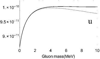
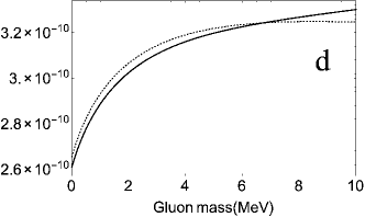
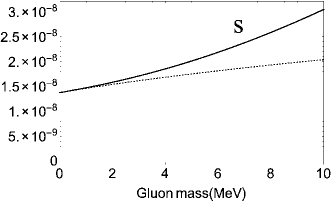
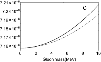
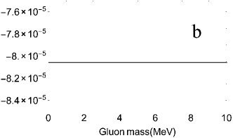
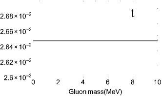
Figure 6: $4mF_{2}$ of quarks at $q^{2}=-M^{2}_{Z}$ ; continuous lines represent dependence on topologically generated gluon mass; dotted lines represent dependence on gluon mass coming from a Proca term.

Finally, in Fig. 7 we have plotted $4mF_{2}$ for each quark, at both the scales $m_{t}$ and $M_{Z}$, against topologically generated gluon mass.

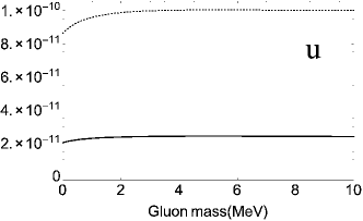
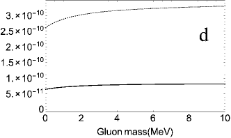
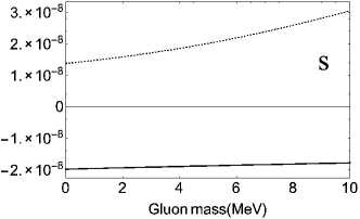
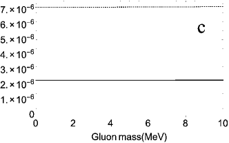
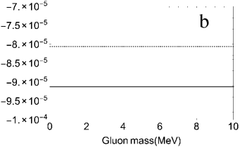
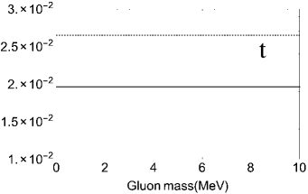
Figure 7: $4mF_{2}$ of quarks ; continuous lines represent dependence on topologically generated gluon mass at $q^{2}=-m^{2}_{t}$ ; dotted lines represent dependence on gluon mass at $q^{2}=-M^{2}_{z}$ .

III Results and Discussions

In this paper we have considered a specific model of gauge-invariant mass generation, namely the topologically massive gauge theory, and calculated the anomalous chromomagnetic moment $F_{2}(q^{2})\,,$ at the energy scale $M_{Z}$ as well as at $m_{t}$ . Looking at Fig. 6 we see that gluon mass dependence of the ACM is the most prominent for the strange quark. As the gluon mass is increased from 0 to 10 MeV, the dimensionless quantity $4mF_{2}(q^{2}=-M_{Z}^{2})$ varies by more than $100\%$ for the $s$-quark when the gluon mass is topologically generated. For a Proca mass term this variation is only about $42\%$. On the other hand, for the top and bottom quarks the mass dependence of the ACM is negligible over this mass range, irrespective of the mechanism responsible for mass generation (for the $b$ quark the variation is about 0.1%, for the $t$ quark even less). Among the heavy quarks, the charm quark shows approximately $0.5\%$ variation, almost the same for both topological and Proca mass terms. For the up and down quarks, the ACM varies by about 20 – 25% when the gluon mass is varied over 0 – 10 MeV, and is higher for the topological mass term by about 2% at the top of the range.

Next we take a look at Fig. 7. Here we have plotted the dimensionless quantity $4mF_{2}$ of quarks at two different values of $q^{2}$ for the same range of topologically generated gluon mass. We have plotted $4mF_{2}$ at the scale $m_{t}$ as continuous lines, and $4mF_{2}$ at the scale $M_{Z}$ as dotted lines, against gluon mass between 0 and 10 MeV. From these plots, we see that the gluon mass dependence of $4mF_{2}$ is more pronounced at $q^{2}=-M^{2}_{Z}$ than at $q^{2}=-m^{2}_{t}$ for the light quarks like up, down and strange. For the top and bottom quarks, the gluon mass dependence is negligible for both the energy scales $q^{2}=-M_{Z}^{2}$ and $q^{2}=-m_{t}^{2}$ although the actual values of the ACM are largely different at the two energy scales.

What we can conclude from all this is that the ACM of the light quarks have significant, and possibly observable, dependence on gluon mass, irrespective of how the mass is generated. As higher energies and luminosities become accessible to the LHC, precision measurements of the anomalous chromomagnetic moments of quarks should become possible. While a measurement of the top quark ACM is unlikely to constrain the gluon mass, data for other quarks will be able to put bounds on the mass of the gluon.

Appendix A Calculations

This section contains some details of the calculations for Eq. (16)-(21). Let us start with $\Gamma^{(1)}_{\mu}$  as given in Eq. (16). We can write it in the form

$$\Gamma^{(1)}_{\mu}=3!\int\limits_{0}^{1}d\zeta_{1}\int\limits_{0}^{1}d\zeta_{2}\int\limits_{0}^{1}d\zeta_{3}\int\limits_{0}^{1}d\zeta_{4}\int\dfrac{d^{4}k}{(2\pi)^{4}}\delta(1-\zeta_{1}-\zeta_{2}-\zeta_{3}-\zeta_{4})$$

$$\times\dfrac{N^{(1)}_{\mu}(k+\zeta_{2}p^{\prime}+(\zeta_{3}+\zeta_{4})p)}{[k^{2}-(\zeta_{2}+\zeta_{3}+\zeta_{4})^{2}m^{2}+\zeta_{2}(\zeta_{3}+\zeta_{4})q^{2}+(-\zeta_{1}+\zeta_{2}+\zeta_{3}+\zeta_{4})m^{2}-(\zeta_{2}+\zeta_{3})M^{2}]^{4}}\,,$$ (25)

where we have defined

$$N_{\mu}^{(1)}(k)=(p-k)_{\mu}\gamma_{\lambda}(\hbox to0.0pt{\hbox to5.52084pt{\hfil/\hfil}\hss}k+m)\gamma^{\lambda}-(\hbox to0.0pt{\hbox to5.03125pt{\hfil/\hfil}\hss}p-\hbox to0.0pt{\hbox to5.52084pt{\hfil/\hfil}\hss}k)(\hbox to0.0pt{\hbox to5.52084pt{\hfil/\hfil}\hss}k+m)\gamma_{\mu}\,.$$ (26)

Similarly, we can write $\Gamma^{(2)}_{\mu}$ as

$$\Gamma^{(2)}_{\mu}=3!\int\limits_{0}^{1}d\zeta_{1}\int\limits_{0}^{1}d\zeta_{2}\int\limits_{0}^{1}d\zeta_{3}\int\limits_{0}^{1}d\zeta_{4}\int\dfrac{d^{4}k}{(2\pi)^{4}}\delta(1-\zeta_{1}-\zeta_{2}-\zeta_{3}-\zeta_{4})$$

$$\times\dfrac{N^{(2)}_{\mu}(k+\zeta_{2}p+(\zeta_{3}+\zeta_{4})p^{\prime})}{[k^{2}-(\zeta_{2}+\zeta_{3}+\zeta_{4})^{2}m^{2}+\zeta_{2}(\zeta_{3}+\zeta_{4})q^{2}+(-\zeta_{1}+\zeta_{2}+\zeta_{3}+\zeta_{4})m^{2}-(\zeta_{2}+\zeta_{3})M^{2}]^{4}}\,,$$ (27)

with

$$N_{\mu}^{(1)}(k)=\gamma_{\mu}(\hbox to0.0pt{\hbox to5.52084pt{\hfil/\hfil}\hss}k+m)(\hbox to0.0pt{\hbox to5.52084pt{\hfil/\hfil}\hss}k-\,/\kern-6.00006pt{p^{\prime}})-\gamma_{\lambda}(\hbox to0.0pt{\hbox to5.52084pt{\hfil/\hfil}\hss}k+m)\gamma^{\lambda}(k-p^{\prime})_{\mu}\,.$$ (28)

Not all terms of this expression will contribute to $F_{2}$. Keeping only the relevant terms of $N_{\mu}^{(1)}(k)$ and $N_{\mu}^{(2)}(k)$ , we find that the sum of the contributions from $\Gamma^{(1)}_{\mu}$ and $\Gamma^{(2)}_{\mu}$ is

$$F^{(1)+(2)}_{2}(q^{2})=\frac{i}{8\pi^{2}m^{3}}\int\limits_{0}^{1}d\zeta_{1}\int\limits_{0}^{1-\zeta_{1}}d\zeta_{2}\int\limits_{0}^{1-\zeta_{1}-\zeta_{2}}d\zeta_{3}\dfrac{\zeta_{1}^{2}}{\left[\zeta_{1}^{2}-\zeta_{2}(1-\zeta_{1}+\zeta_{2})\frac{q^{2}}{m^{2}}-(\zeta_{2}+\zeta_{3})^{2}\frac{M^{2}}{m^{2}}\right]^{2}}\,.$$ (29)

Next we consider $\Gamma^{(3)}_{\mu}$. We can write it as

$$\Gamma^{(3)}_{\mu} =\frac{2}{q^{2}}\int\limits_{0}^{1}d\zeta_{1}\int\limits_{0}^{1}d\zeta_{2}\int\limits_{0}^{1}d\zeta_{3}\int\dfrac{d^{4}k}{(2\pi)^{4}}\delta(1-\zeta_{1}-\zeta_{2}-\zeta_{3})$$

$$\qquad\times\dfrac{N_{\mu}^{(3)}(k+\zeta_{2}p+\zeta_{3}p^{\prime})}{[k^{2}-(\zeta_{2}+\zeta_{3})^{2}m^{2}+\zeta_{2}\zeta_{3}q^{2}+(-\zeta_{1}+\zeta_{2}+\zeta_{3})m^{2}-(\zeta_{2}+\zeta_{3})M^{2}]^{3}}\,,$$ (30)

where we have written

$$N_{\mu}^{(3)}(k)=\gamma_{\mu}(\hbox to0.0pt{\hbox to5.52084pt{\hfil/\hfil}\hss}k+m)\hbox to0.0pt{\hbox to5.00002pt{\hfil$q$\hfil}\hss}/-\hbox to0.0pt{\hbox to5.00002pt{\hfil$q$\hfil}\hss}/(\hbox to0.0pt{\hbox to5.52084pt{\hfil/\hfil}\hss}k+m)\gamma_{\mu}.$$ (31)

The contribution for $\Gamma^{(3)}_{\mu}$ is easily calculated from this to be

$$F^{(3)}_{2}(q^{2})=\frac{i}{8\pi^{2}mq^{2}}\int\limits_{0}^{1}d\zeta_{1}\int\limits_{0}^{1-\zeta_{1}}d\zeta_{2}\dfrac{\zeta_{1}}{\zeta_{1}^{2}-(1-\zeta_{1}-\zeta_{2})\zeta_{2}\frac{q^{2}}{m^{2}}+(1-\zeta_{1})\frac{M^{2}}{m^{2}}}\,.$$ (32)

The remaining three $\Gamma$’s have long expressions. We will show the calculation of $\Gamma^{(4)}_{\mu}$ in some detail, showing only the final expression for the other two. We can write $\Gamma^{(4)}_{\mu}$ as

$$\Gamma^{(4)}_{\mu}=4!\int\limits_{0}^{1}d\zeta_{1}\int\limits_{0}^{1}d\zeta_{2}\int\limits_{0}^{1}d\zeta_{3}\int\limits_{0}^{1}d\zeta_{4}\int\limits_{0}^{1}d\zeta_{5}\int\dfrac{d^{5}k}{(2\pi)^{4}}\delta(1-\zeta_{1}-\zeta_{2}-\zeta_{3}-\zeta_{4}-\zeta_{5})$$

$$\times\dfrac{N_{\mu}^{(4)}\left(k+(\zeta_{2}+\zeta_{3})p+(\zeta_{4}+\zeta_{5})p^{\prime}\right)}{[k^{2}-(\zeta_{2}+\zeta_{3}+\zeta_{4}+\zeta_{5})^{2}m^{2}+(\zeta_{2}+\zeta_{3})(\zeta_{4}+\zeta_{5})q^{2}+(\zeta_{2}+\zeta_{3}+\zeta_{4}+\zeta_{5}-\zeta_{1})m^{2}-(\zeta_{2}+\zeta_{4})M^{2}]^{5}}\,,$$ (33)

where the function in the numerator is

$$N_{\mu}^{(4)}(k)= -(\hbox to0.0pt{\hbox to5.52084pt{\hfil/\hfil}\hss}k-\hbox to0.0pt{\hbox to5.03125pt{\hfil/\hfil}\hss}p)(\hbox to0.0pt{\hbox to5.52084pt{\hfil/\hfil}\hss}k+m)(\hbox to0.0pt{\hbox to5.52084pt{\hfil/\hfil}\hss}k-\hbox to0.0pt{\hbox to6.57124pt{\hfil/\hfil}\hss}p^{\prime})(2k-p-p^{\prime})_{\mu}+2(k-p)_{\mu}(\hbox to0.0pt{\hbox to5.52084pt{\hfil/\hfil}\hss}k-\hbox to0.0pt{\hbox to6.57124pt{\hfil/\hfil}\hss}p^{\prime})(\hbox to0.0pt{\hbox to5.52084pt{\hfil/\hfil}\hss}k+m)(\hbox to0.0pt{\hbox to5.52084pt{\hfil/\hfil}\hss}k-\hbox to0.0pt{\hbox to6.57124pt{\hfil/\hfil}\hss}p^{\prime})$$

$$+2(k-p^{\prime})_{\mu}(\hbox to0.0pt{\hbox to5.52084pt{\hfil/\hfil}\hss}k-\hbox to0.0pt{\hbox to5.03125pt{\hfil/\hfil}\hss}p)(\hbox to0.0pt{\hbox to5.52084pt{\hfil/\hfil}\hss}k+m)(\hbox to0.0pt{\hbox to5.52084pt{\hfil/\hfil}\hss}k-\hbox to0.0pt{\hbox to5.03125pt{\hfil/\hfil}\hss}p)-(k-p^{\prime})\cdot(k-p)\{2(\hbox to0.0pt{\hbox to5.52084pt{\hfil/\hfil}\hss}k-\hbox to0.0pt{\hbox to6.57124pt{\hfil/\hfil}\hss}p^{\prime})(\hbox to0.0pt{\hbox to5.52084pt{\hfil/\hfil}\hss}k+m)\gamma_{\mu}$$

$$-\gamma_{\lambda}(\hbox to0.0pt{\hbox to5.52084pt{\hfil/\hfil}\hss}k+m)\gamma^{\lambda}(2k-p-p^{\prime})_{\mu}+2\gamma_{\mu}(\hbox to0.0pt{\hbox to5.52084pt{\hfil/\hfil}\hss}k+m)(\hbox to0.0pt{\hbox to5.52084pt{\hfil/\hfil}\hss}k-\hbox to0.0pt{\hbox to5.03125pt{\hfil/\hfil}\hss}p)\}\,.$$ (34)

Changing variables from $k$ to $k+(\zeta_{2}+\zeta_{3})p+(\zeta_{4}+\zeta_{5})p^{\prime}\,,$ we can write the first term in Eq. (34) as

$$-(\hbox to0.0pt{\hbox to5.52084pt{\hfil/\hfil}\hss}k+\hbox to0.0pt{\hbox to5.28589pt{\hfil/\hfil}\hss}a-\hbox to0.0pt{\hbox to5.03125pt{\hfil/\hfil}\hss}p)(\hbox to0.0pt{\hbox to5.52084pt{\hfil/\hfil}\hss}k+\hbox to0.0pt{\hbox to5.28589pt{\hfil/\hfil}\hss}a+m)(\hbox to0.0pt{\hbox to5.52084pt{\hfil/\hfil}\hss}k+\hbox to0.0pt{\hbox to5.28589pt{\hfil/\hfil}\hss}a-\hbox to0.0pt{\hbox to6.57124pt{\hfil/\hfil}\hss}p^{\prime})\{2k+(2\zeta_{2}+2\zeta_{3}-1)p+(2\zeta_{3}+2\zeta_{4}-1)p^{\prime}\}_{\mu}\,,$$ (35)

where we have defined

$$a_{\mu}=(\zeta_{2}+\zeta_{3})p_{\mu}+(\zeta_{3}+\zeta_{4})p^{\prime}_{\mu}\,.$$ (36)

As before, we ignore terms in Eq. (35) which do not contribute to $F_{2}(q^{2})$. The relevant terms can then be written as

$$-\frac{1}{2}mk^{2}\left({3}(A+B)-2\right)b_{\mu}+mk^{2}(1-A-B)a_{\mu}$$

$$\qquad\qquad+(1-A-B)mb_{\mu}\left[\left((A+B)^{2}-1\right)m^{2}+(1-AB)q^{2}\right]\,,$$ (37)

where we have written

$$A=\zeta_{2}+\zeta_{3}\,,\qquad B=\zeta_{4}+\zeta_{5}\,,$$ (38)

and

$$b_{\mu}=(2A-1)p_{\mu}+(2B-1)p^{\prime}_{\mu}\,.$$ (39)

The second and third terms in Eq. (34), when added together, produce

$$2(\hbox to0.0pt{\hbox to5.52084pt{\hfil/\hfil}\hss}k-m)(k^{2}-m^{2})(2k-p-p^{\prime})\,.$$ (40)

After transforming from $k$ to $k+(\zeta_{2}+\zeta_{3})p+(\zeta_{4}+\zeta_{5})p^{\prime}$ , we can write the relevant terms in Eq. (40) as

$$-mk^{2}a_{\mu}(1-A-B) +mb_{\mu}[k^{2}\left((A+B)-2\right)$$

$$+m^{2}(1-A-B)^{2}(1+A+B)+AB(1-A-B)q^{2}]\,.$$ (41)

It is easy to see that the fourth and the last terms in Eq. (34) do not contribute. The relevant expression contributed by the fifth term of Eq. (34) are

$$[-2k^{2}-2m^{2}(1-A-B)^{2}+\left(AB+(A-1)(B-1)\right)q^{2}](A+B-2)mb_{\mu}\,.$$ (42)

Adding Eq. (35), (41) and (42)and their forms obtained by interchanging dummy variables $\zeta_{2}$, $\zeta_{4}$ and $\zeta_{3}$, $\zeta_{5}$, we get from $N_{\mu}^{(4)}(k)$ ,

$$\left[-3(1-A-B)mk^{2}-2(1-A-B)^{3}(2-A-B)m^{3}\right.$$

$$\qquad\left.+\left((1-A-B)^{3}+2AB(1-A-B)(2-A-B)\right)mq^{2}\right](p+p^{\prime})_{\mu}\,.$$ (43)

Using Gordon’s identity, we find that the contribution to $F_{2}(q^{2})$ from $\Gamma^{(4)}_{\mu}$ can be written as

$$F^{(4)}_{2}(q^{2})= -\dfrac{i}{8\pi^{2}m^{3}}\int\limits_{0}^{1}d\zeta_{1}\int\limits_{0}^{1}d\zeta_{2}\int\limits_{0}^{1}d\zeta_{3}\int\limits_{0}^{1}d\zeta_{4}\int\limits_{0}^{1}d\zeta_{5}\,\delta(1-\zeta_{1}-\zeta_{2}-\zeta_{3}-\zeta_{4}-\zeta_{5})$$

$$\times\left[\dfrac{3(1-\zeta_{2}-\zeta_{3}-\zeta_{4}-\zeta_{5})}{\left[(1-\zeta_{2}-\zeta_{3}-\zeta_{4}-\zeta_{5})^{2}-(\zeta_{2}+\zeta_{3})(\zeta_{4}+\zeta_{5})\frac{q^{2}}{m^{2}}+(\zeta_{2}+\zeta_{4})\frac{M^{2}}{m^{2}}\right]^{2}}\right.$$

$$+\dfrac{2(1-\zeta_{2}-\zeta_{3}-\zeta_{4}-\zeta_{5})^{3}(\zeta_{2}+\zeta_{3}+\zeta_{4}+\zeta_{5}-2)}{\left[(\zeta_{2}+\zeta_{3}+\zeta_{4}+\zeta_{5})^{2}-(\zeta_{2}+\zeta_{3})(\zeta_{4}+\zeta_{5})\frac{q^{2}}{m^{2}}-(\zeta_{2}+\zeta_{3}+\zeta_{4}+\zeta_{5}-\zeta_{1})+(\zeta_{2}+\zeta_{4})\frac{M^{2}}{m^{2}}\right]^{3}}$$

$$\left.+\dfrac{q^{2}}{m^{2}}\dfrac{(1-\zeta_{2}-\zeta_{3}-\zeta_{4}-\zeta_{5})\left[2(2-\zeta_{2}-\zeta_{3}-\zeta_{4}-\zeta_{5})(\zeta_{2}+\zeta_{3})(\zeta_{4}+\zeta_{5})+(1-\zeta_{2}-\zeta_{3}-\zeta_{4}-\zeta_{5})^{2}\right]}{\left[(\zeta_{2}+\zeta_{3}+\zeta_{4}+\zeta_{5})^{2}-(\zeta_{2}+\zeta_{3})(\zeta_{4}+\zeta_{5})\frac{q^{2}}{m^{2}}-(\zeta_{2}+\zeta_{3}+\zeta_{4}+\zeta_{5}-\zeta_{1})+(\zeta_{2}+\zeta_{4})\frac{M^{2}}{m^{2}}\right]^{3}}\right]\,.$$ (44)

We can calculate the contributions from $\Gamma^{(5)}_{\mu}$ and $\Gamma^{(6)}_{\mu}$ in a similar manner, and their sum has a fairly simple expression,

$$F^{(5)+(6)}_{2}(q^{2})= -\dfrac{i}{4\pi^{2}m^{3}}\int\limits_{0}^{1}d\zeta_{1}\int\limits_{0}^{1}d\zeta_{2}\int\limits_{0}^{1}d\zeta_{3}\int\limits_{0}^{1}d\zeta_{4}\,\delta(1-\zeta_{1}-\zeta_{2}-\zeta_{3}-\zeta_{4})$$

$$\times\dfrac{\zeta_{2}(\zeta_{2}+\zeta_{3}+\zeta_{4}-1)}{\left[(\zeta_{2}+\zeta_{3}+\zeta_{4})^{2}-\zeta_{2}(\zeta_{3}+\zeta_{4})\frac{q^{2}}{m^{2}}-(-\zeta_{1}+\zeta_{2}+\zeta_{3}+\zeta_{4})+(\zeta_{2}+\zeta_{3})\frac{M^{2}}{m^{2}}\right]^{2}}\,.$$ (45)

References

(1)
W. Bernreuther, D. Heisler and Z. G. Si,
A set of top quark spin correlation and polarization observables for the LHC: Standard Model predictions and new physics contributions,
arXiv:1508.05271 [hep-ph].
(2)
D. Buarque Franzosi and C. Zhang,
Phys. Rev. D 91, 114010 (2015).
(3)
N. I. Kochelev,
Phys. Lett. B 426, 149 (1998).
(4)
N. Kochelev and N. Korchagin,
Phys. Lett. B 729, 117 (2014).
(5)
N. Kochelev and N. Korchagin,
Phys. Rev. D 89, 034028 (2014).
(6)
L. Chang, Y. X. Liu and C. D. Roberts,
Phys. Rev. Lett. 106, 072001 (2011).
(7)
S. D. Rindani, P. Sharma and A. W. Thomas,
Polarization of top quark as a probe of its chromomagnetic and chromoelectric couplings in production at the Large Hadron Collider,
arXiv:1507.08385 [hep-ph].
(8)
Z. Hioki and K. Ohkuma,
Eur. Phys. J. C 65, 127 (2010).
(9)
Z. Hioki and K. Ohkuma,
Eur. Phys. J. C 71, 1535 (2011).
(10)
Z. Hioki and K. Ohkuma,
Phys. Rev. D 88, 017503 (2013).
(11)
J. F. Kamenik, M. Papucci and A. Weiler,
Phys. Rev. D 85, 071501 (2012).
(12)
R. Martínez and J. A. Rodríguez,
Phys. Rev. D 55, 3212 (1997).
(13)
R. Martínez and J. A. Rodríguez,
Phys. Rev. D 65, 057301 (2002).
(14)
R. Martinez, M. A. Perez and N. Poveda,
Eur. Phys. J. C 53, 221 (2008).
(15)
R. Gaitan, E. A. Garces, J. H. M. de Oca and R. Martinez,
Top quark Chromoelectric and Chromomagnetic Dipole Moments in a Two Higgs Doublet Model with CP violation,
arXiv:1505.04168 [hep-ph].
(16)
D. Choudhury and P. Saha,
JHEP 1208, 144 (2012)
(17)
L. Labun and J. Rafelski,
Higgs two-gluon decay and the top-quark chromomagnetic moment,
arXiv:1210.3150 [hep-ph].
(18)
C. Degrande, J. M. Gerard, C. Grojean, F. Maltoni and G. Servant,
JHEP 1207, 036 (2012)
[Erratum-ibid. 1303, 032 (2013)]
(19)
S. Y. Ayazi, H. Hesari and M. M. Najafabadi,
Phys. Lett. B 727, 199 (2013)
(20)
H. Hesari and M. Mohammadi Najafabadi,
Phys. Rev. D 91, 057502 (2015).
(21)
S. S. Biswal, S. D. Rindani and P. Sharma,
Phys. Rev. D 88, 074018 (2013)
(22)
CMS Collaboration [CMS Collaboration],
Search for Anomalous Top Chromomagnetic Dipole Moments from angular distributions in Dileptonic events at TeV with the CMS detector,
CMS-PAS-TOP-14-005 (2014).
(23)
J. Beringer et al. [Particle Data Group Collaboration],
Review of Particle Physics (RPP),
Phys. Rev. D 86, 010001 (2012) and
2013 partial update for the 2014 edition.
(24)
J. M. Cornwall,
Phys. Rev. D 26, 1453 (1982).
(25)
A. C. Aguilar and J. Papavassiliou,
Phys. Rev. D 81, 034003 (2010).
(26)
G. Parisi and R. Petronzio,
Phys. Lett. B 94, 51 (1980).
(27)
J. H. Field,
Phys. Rev. D 66, 013013 (2002).
(28)
F. J. Yndurain,
Phys. Lett. B 345, 524 (1995).
(29)
S. Nussinov and R. Shrock,
Phys. Rev. D 82, 034031 (2010).
(30)
G. Curci and R. Ferrari,
Nuovo Cim. A 32, 151 (1976).
(31)
J. de Boer, K. Skenderis, P. van Nieuwenhuizen and A. Waldron,
Phys. Lett. B 367, 175 (1996).
(32)
T. J. Allen, M. J. Bowick and A. Lahiri,
Mod. Phys. Lett. A 6, 559 (1991).
(33)
D. S. Hwang and C. Lee,
J. Math. Phys. 38, 30 (1997).
(34)
A. Lahiri,
Phys. Rev. D 55, 5045 (1997).
(35)
I. D. Choudhury and A. Lahiri,
Mod. Phys. Lett. A 30, 1550113 (2015).