A BP-MF-EP Based Iterative Receiver for Joint Phase Noise Estimation, Equalization and Decoding

Abstract

In this work, with combined belief propagation (BP), mean field (MF) and expectation propagation (EP), an iterative receiver is designed for joint phase noise (PN) estimation, equalization and decoding in a coded communication system. The presence of the PN results in a nonlinear observation model. Conventionally, the nonlinear model is directly linearized by using the first-order Taylor approximation, e.g., in the state-of-the-art soft-input extended Kalman smoothing approach (soft-in EKS). In this work, MF is used to handle the factor due to the nonlinear model, and a second-order Taylor approximation is used to achieve Gaussian approximation to the MF messages, which is crucial to the low-complexity implementation of the receiver with BP and EP. It turns out that our approximation is more effective than the direct linearization in the soft-in EKS with similar complexity, leading to significant performance improvement as demonstrated by simulation results.

I Introduction

Local oscillators, which provide a reference signal for time and frequency synchronization, are one of the key modules in a communication system. The instability of oscillators results in phase noise (PN), which may severely affect the system performance [1].

Various Bayesian and non-Bayesian approaches have been proposed to solve the PN problem. Bhatti et al. modelled the PN with a discrete cosine transform (DCT) expansion [2], where the DCT coefficients can be easily estimated. However, the DCT method is a non-Bayesian one, and it does not make use of the time dependence of the PN process. In Bayesian methods such as particle filter [3], Tikhonov parametric estimation [4], and extended Kalman smoothing (EKS) [5], PN is modelled as a Wiener process. The particle filtering method [3] needs to sample the posteriori probability density function (PDF) of continuous-valued PN variables, where a larger number of particles yields better performance at the cost of higher complexity. The Tikhonov parametrization method [4] (or called a von Mises distribution [6]) is an iterative method to deal with the presence of strong PN for AWGN channels. The intractable integral operation associated with continuous variables is circumvented by constraining the PDF to Tikhonov distribution. However, the work in [4] was focused on AWGN channel, and a straightforward extension to the inter-symbol interference (ISI) channel which is allowed by incorporating a MAP equalizer will lead to complexity growing exponentially with the channel memory length. In the soft input EKS (Soft-in EKS) method proposed in  [5], the nonlinear observation model is directly linearized by using the first order Taylor expansion. Soft-in EKS has been used in single-input single-output (SISO) and multiple-input multiple-output (MIMO) systems [5, 8, 9, 10].

Recently, the message passing techniques, such as belief propagation (BP) [11] and variational message passing (VMP) [12], have been widely used for iterative receivers design. BP is effective for discrete probability models and linear Gaussian models. A BP-based equalizer proposed in [13] has a linear complexity, which is much lower than that of the equalizer in [14]. The VMP method, also referred as mean filed (MF), is especially suitable for handling variables with exponential distributions. Recently, a unified message passing framework was proposed in [15], where BP and MF are merged to keep the virtues of BP and MF while avoid their drawbacks. It has been applied to joint channel estimation and decoding in orthogonal frequency division multiplexing (OFDM) system [16],[17] and single carrier frequency domain equalization (SC-FDE) system [18]. In addition, expectation propagation (EP)[19] has been used to achieve Gaussian approximation to non-Gaussian messages, and combined EP and BP has been applied to flat-fading or ISI channel equalization, e. g., in [20, 7] .

In this paper, with combined BP, MF and EP, we propose an iterative approach to joint PN estimation, equalization and decoding for a coded system over ISI channels. BP and EP are used to deal with the linear model for PN process and modulation and coding, while MF is used to handle the factor due to the nonlinear observation model. Furthermore, the non-Gaussian MF messages are approximated to be Gaussian by using the second-order Taylor expansion, which enables low-complexity implementation of the receiver with BP and EP. Our approximation is more effective than the direct linearization of the nonlinear model in the soft-in EKS [5], which is demonstrated by the significant performance gain of the proposed approach in terms of mean-square-error (MSE) of PN estimation and system bit-error-rate (BER) performance.

Notation-The superscriptions $(\cdot)^{\textrm{T}}$and $(\cdot)^{\text{H}}$denote the transpose and conjugate transpose, respectively. We use $\propto$ to denote equality of functions up to a scale factor, and use $\boldsymbol{I}_{N}$ to denote an $N\times N$ identity matrix. The real part of a complex quantity is denoted by $\Re[\cdot]$. The functions $\mathcal{N}(x;\hat{x},\sigma^{2}_{x})$ and $\mathcal{CN}(x;\hat{x},\sigma^{2}_{x})$ stand for real and proper complex Gaussian probability distributions with mean $\hat{x}$ and variance $\sigma^{2}_{x}$, respectively.

II System Model and Factor Graph Representation

We consider a coded communication system. An information bit sequence $\boldsymbol{b}=[b_{0},...,b_{N_{b}-1}]^{\textrm{T}}$ is encoded and interleaved, yielding an interleaved codeword $\boldsymbol{c}=[c_{0},...,c_{N_{c}-1}]^{\textrm{T}}$. Then sequence $\boldsymbol{c}$ is mapped to a symbol sequence $\boldsymbol{x}=[x_{0},...,x_{M-1}]^{\textrm{T}}$ which is transmitted over an ISI channel with coefficients $\boldsymbol{h}=[h_{L-1},...,h_{0}]^{\textrm{T}}$. The channel coefficients are assumed to be constant during each transmitted block and they are available to the receiver. By considering the effect of PN, the received baseband signal at time instant $k$, $(k=0,1,...,M+L-2)$, can be represented as[21]

$$y_{k}=e^{j\theta_{k}}\sum_{l=0}^{L-1}h_{l}x_{k-l}+n_{k}=e^{j\theta_{k}}\boldsymbol{h}^{\textrm{T}}\boldsymbol{s}_{k}+n_{k}$$ (1)

where $\boldsymbol{s}_{k}\triangleq[x_{k-L+1},...,x_{k}]^{\textrm{T}}$ with $x_{k}=0$ for $k<0$ and $k>M-1$, and $n_{k}$ is a sample of the complex Gaussian noise with variance $\sigma_{n}^{2}$. The phase $\theta_{k}$ represents the PN at time instant $k$, and the PN can be modelled as a random-walk (Wiener) process [4], [5]

$$\theta_{k}=\theta_{k-1}+\Delta\theta_{k}$$ (2)

where $\Delta\theta_{k}$ is a white real Gaussian process with distribution $\mathcal{N}(\Delta\theta_{k};0,\sigma^{2}_{\Delta})$, and $\theta_{0}$ is assumed to have a uniform distribution over $[0,2\pi)$. We define $\boldsymbol{\theta}=[\theta_{0},\theta_{1},...,\theta_{M+L-2}]^{\textrm{T}}$.

The joint probability of $\boldsymbol{b,c,x,s}$ and $\boldsymbol{\theta}$ with given observation $\boldsymbol{y}=[y_{0},y_{1},\dots,y_{M+L-2}]^{\textrm{T}}$ can be expressed as

$$p(\boldsymbol{b},\boldsymbol{c},\boldsymbol{x},\boldsymbol{s},\boldsymbol{\theta}|\boldsymbol{y})\propto \prod_{k=0}^{M+L-2}f_{y_{k}}(\boldsymbol{s}_{k},\theta_{k})f_{\boldsymbol{s}_{k}}(\boldsymbol{s}_{k},\boldsymbol{s}_{k-1},x_{k})$$

$$f_{\theta_{0}}\prod_{k=1}^{M+L-2}f_{\theta_{k}}(\theta_{k},\theta_{k-1})f_{\textrm{X}}(\boldsymbol{x},\boldsymbol{c},\boldsymbol{b})$$ (3)

where $f_{y_{k}}(\boldsymbol{s}_{k},\theta_{k})\triangleq p(y_{k}|\boldsymbol{s}_{k},\theta_{k})\propto\mathcal{CN}(y_{k};e^{j\theta_{k}}\boldsymbol{h}^{\textrm{T}}\boldsymbol{s}_{k},\sigma_{n}^{2})$ denotes the likelihood function of $\boldsymbol{s}_{k}$ and $\boldsymbol{\theta}_{k}$, $f_{\theta_{k}}(\theta_{k},\theta_{k-1})\triangleq p(\theta_{k}|\theta_{k-1})=\mathcal{N}(\theta_{k};\theta_{k-1},\sigma^{2}_{\Delta})$ is the conditional PDF of $\theta_{k}$ given $\theta_{k-1}$, and $f_{\textrm{X}}(\boldsymbol{x},\boldsymbol{c},\boldsymbol{b})$ denotes the mapping, interleaving and coding constraints. Function $f_{s_{k}}\left(\boldsymbol{s}_{k},\boldsymbol{s}_{k-1},x_{k}\right)$ represents the deterministic relationship between $\boldsymbol{s}_{k}$, $\boldsymbol{s}_{k-1}$ and $x_{k}$ which is given by $\boldsymbol{s}_{k}=\boldsymbol{G}\boldsymbol{s}_{k-1}+\boldsymbol{e}x_{k}$, where the $L\times L$ matrix $\boldsymbol{G}=[\boldsymbol{0}\ \boldsymbol{I}_{L-1};\ 0\ \boldsymbol{0}^{\textrm{T}}]$, the length-$L$ vector $\boldsymbol{e}=[\boldsymbol{0}^{\textrm{T}}\ 1]^{\textrm{T}}$, and $\boldsymbol{0}$ is a zero column vector with length $L-1$.

A factor graph representation of (3) is shown in Fig. 1, which will be employed to develop a combined BP-MF-EP based receiver to achieve joint PN estimation, equalization and decoding in next section.

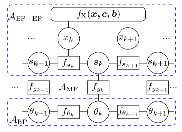
Figure 1: Factor-graph representation of the probabilistic model (3)

III Iterative Receiver Design with BP-MF-EP

Due to the presence of PN, the observation model in (1) is nonlinear. In EKS, the nonlinear model is directly linearized with the first order Taylor approximation. The nonlinear model is represented by the factors $\{f_{y_{k}},\forall k\}$ in Fig. 1. In this work, we use MF to handle the factors.

As shown in Fig. 1, we partition the graph into three parts: BP-EP subgraph, MF subgraph and BP subgraph. Accordingly, the factor nodes are classified into three disjoint sets: $\mathcal{A}_{\textrm{BP-EP}}\triangleq\{f_{s_{k}},f_{\textrm{X}};\forall k\}$, $\mathcal{A}_{\textrm{MF}}\triangleq\{f_{y_{k}};\forall k\}$ and $\mathcal{A}_{\textrm{BP}}\triangleq\{f_{\theta_{k}};\forall k\}$ with $\mathcal{A}_{\textrm{BP-EP}}\bigcap\mathcal{A}_{\textrm{MF}}\bigcap\mathcal{A}_{\textrm{BP}}=\emptyset$. In the following, we detail the messages updating in each subgraph.

III-A Message Passing in BP Subgraph

As shown in Fig. 1, message passing for PN estimation operates in the BP subgraph, where we need to calculate the forward and backward messages and the outgoing messages which are input to the MF subgraph.

We assume that the incoming messages from the MF subgraph are available, and they are Gaussian, i.e., we have $\{m_{f_{y_{k}}\to\theta_{k}}\left(\theta_{k}\right)\propto\mathcal{N}(\theta_{k};\hat{\theta}^{\downarrow}_{k},\sigma^{2}_{\theta^{\downarrow}_{k}}),\forall k\}$. The details on the calculations of the incoming messages are delayed to Section III-C. It is worth mentioning that, with the incoming Gaussian messages, all the messages running in the subgraph are Gaussian.

With the Gaussian message $m_{f_{\theta_{k-1}}\to\theta_{k-1}}(\theta_{k-1})$ $\propto\mathcal{N}(\theta_{k-1};\hat{\theta}^{\rightarrow}_{k-1},\sigma^{2}_{\theta_{k-1}^{\rightarrow}})$, the message from variable $\theta_{k-1}$ to factor $f_{\theta_{k}}$ is calculated as $n_{\theta_{k-1}\to f_{\theta_{k}}}(\theta_{k-1})=m_{f_{\theta_{k-1}}\to\theta_{k-1}}(\theta_{k-1})m_{f_{y_{k-1}}\to\theta_{k-1}}(\theta_{k-1})$. The forward message $m_{f_{\theta_{k}}\to\theta_{k}}(\theta_{k})$ reads

$$m_{f_{\theta_{k}}\to\theta_{k}}(\theta_{k}) \propto\int f_{\theta_{k}}(\theta_{k},\theta_{k-1})n_{\theta_{k-1}\to f_{\theta_{k}}}(\theta_{k-1})d\theta_{k-1}$$

$$\propto\mathcal{N}(\theta_{k};\hat{\theta}^{\rightarrow}_{k},\sigma^{2}_{\theta_{k}^{\rightarrow}}),$$ (4)

We assume that the initial phase noise $\theta_{0}$ is absorbed into the channel in the acquisition of the channel state information [8], so the initial message for the forward recursive process $\hat{\theta}_{0}=0,\sigma^{2}_{\theta_{0}}=0$.

Same to the forward messages, the backward message $m_{f_{\theta_{k+1}}\to\theta_{k}}(\theta_{k})\propto\mathcal{N}(\theta_{k};\hat{\theta}^{\leftarrow}_{k},\sigma^{2}_{\theta_{k}^{\leftarrow}})$.

According to [15], the outgoing messages input to the MF subgraph should be the belief of $\theta_{k}$, which can be calculated as

$$b(\theta_{k}) =m_{f_{y_{k}}\to\theta_{k}}(\theta_{k})m_{f_{\theta_{k}}\to\theta_{k}}(\theta_{k})m_{f_{\theta_{k+1}}\to\theta_{k}}(\theta_{k})$$

$$\propto\mathcal{N}(\theta_{k};\hat{\theta}_{k},\sigma^{2}_{\theta_{k}}),$$ (5)

where

$$\sigma^{-2}_{\theta_{k}}=\sigma^{-2}_{\theta_{k}^{\downarrow}}+\sigma^{-2}_{\theta_{k}^{\leftarrow}}+\sigma^{-2}_{\theta_{k}^{\rightarrow}}$$ (6)

$$\hat{\theta}_{k}=\sigma^{2}_{\theta_{k}}(\sigma^{-2}_{\theta_{k}^{\downarrow}}\hat{\theta}_{k}^{\downarrow}+\sigma^{-2}_{\theta_{k}^{\leftarrow}}\hat{\theta}_{k}^{\leftarrow}+\sigma^{-2}_{\theta_{k}^{\rightarrow}}\hat{\theta}_{k}^{\rightarrow}).$$ (7)

III-B Message Passing in BP-EP Subgraph

We assume that the incoming messages from the MF subgraph are available, and they are Gaussian. The calculations of the incoming messages will be detailed in Section III-C. So this subgraph involves the incoming Gaussian messages from the MF subgraph and discrete binary messages from the decoder. For this subgraph, we simply borrow the BP-EP algorithm developed in [7] where the use of EP produces Gaussian messages for ${x_{k}}$, which will in turn lead to Gaussian output messages in the BP-EP subgraph. We refer readers to  [7] for the details of the BP-EP algorithm.

With the BP-EP algorithm, we can calculate the messages $m_{f_{\boldsymbol{s}_{k}}\rightarrow\boldsymbol{s}_{k}}(\boldsymbol{s}_{k})\propto\mathcal{CN}(s_{k};\hat{\boldsymbol{s}}^{\rightarrow}_{k},\Sigma_{\boldsymbol{s}^{\rightarrow}_{k}})$ and $m_{f_{\boldsymbol{s}_{k+1}}\rightarrow\boldsymbol{s}_{k}}(\boldsymbol{s}_{k})\propto(s_{k};\hat{\boldsymbol{s}}^{\leftarrow}_{k},\Sigma_{\boldsymbol{s}^{\leftarrow}_{k}})$, which are all Gaussian.

According to [15], the outgoing messages are the belief of $\boldsymbol{s}_{k}$ denoted by $b(\boldsymbol{s}_{k})$, which are Gaussian again and can be expressed as

$$n_{\boldsymbol{s}_{k}\rightarrow f_{y_{k}}}(\boldsymbol{s}_{k}) \propto m_{f_{y_{k}}\rightarrow\boldsymbol{s}_{k}}(\boldsymbol{s}_{k})m_{f_{\boldsymbol{s}_{k}}\rightarrow\boldsymbol{s}_{k}}(\boldsymbol{s}_{k})m_{f_{\boldsymbol{s}_{k+1}}\rightarrow\boldsymbol{s}_{k}}(\boldsymbol{s}_{k})$$

$$\propto\exp\left\{-(\boldsymbol{s}_{k}-\hat{\boldsymbol{s}}_{k})^{\textrm{H}}\Sigma^{-1}_{\hat{\boldsymbol{s}}_{k}}(\boldsymbol{s}_{k}-\hat{\boldsymbol{s}}_{k})\right\}$$ (8)

where $m_{f_{y_{k}}\rightarrow\boldsymbol{s}_{k}}(\boldsymbol{s}_{k})$ is obtained by (15) and

$$\Sigma^{-1}_{\boldsymbol{s}_{k}}=\Sigma^{-1}_{\boldsymbol{s}^{\rightarrow}_{k}}+\Sigma^{-1}_{\boldsymbol{s}^{\uparrow}_{k}}+\Sigma^{-1}_{\boldsymbol{s}^{\leftarrow}_{k}}$$ (9)

$$\Sigma^{-1}_{\boldsymbol{s}_{k}}\hat{\boldsymbol{s}}_{k}=\Sigma^{-1}_{\boldsymbol{s}^{\rightarrow}_{k}}\hat{\boldsymbol{s}}^{\rightarrow}_{k}+\Sigma^{-1}_{\boldsymbol{s}^{\uparrow}_{k}}\hat{\boldsymbol{s}}^{\uparrow}_{k}+\Sigma^{-1}_{\boldsymbol{s}^{\leftarrow}_{k}}\hat{\boldsymbol{s}}^{\leftarrow}_{k}.$$ (10)

III-C Message Passing in the MF Subgraph

As shown by the middle part of the graph in Fig. 1, the MF subgraph consists of the observation factors $f_{y_{k}}$. We need to compute the outgoing messages to the BP-EP subgraph (BP subgraph) based on the incoming messages from the BP subgraph (BP-EP subgraph).

Assume that the incoming message $b(\boldsymbol{s}_{k})$ from the BP-EP subgraph is available. According to the rules [15] the outgoing messages to the BP subgraph can be computed as

$$m_{f_{y_{k}}\rightarrow\theta_{k}}(\theta_{k}) \propto\exp\left\{\int\log(f_{y_{k}}(\theta_{k},\boldsymbol{s}_{k}))b(\boldsymbol{s}_{k})d\boldsymbol{s}_{k}\right\}$$

$$\propto{\exp\left\{\Re[r_{k}e^{j\theta_{k}}]\right\}}$$ (11)

where $r_{k}\triangleq 2\sigma^{-2}_{n}y_{k}^{*}\boldsymbol{h}^{\textrm{T}}\hat{\boldsymbol{s}}_{k}$, and $\hat{\boldsymbol{s}}_{k}$ is the mean parameter vector of the Gaussian belief $b(\boldsymbol{s}_{k})$. Note that the message $m_{f_{y_{k}}\rightarrow\theta_{k}}(\theta_{k})$ yielded in (11) is no longer Gaussian. However, Gaussian messages are expected for the BP subgraph for PN estimation, which is crucial to its low complexity implementation. To achieve this, we use the second-order Taylor expansion of $\Re[r_{k}e^{j\theta_{k}}]$ at the estimate of ${\theta_{k}}$, i.e.,

$$m_{f_{y_{k}}\rightarrow\theta_{k}}(\theta_{k})$$

$$\approx\exp\left\{-\frac{1}{2}\Re[r_{k}e^{j\hat{\theta}_{k}}]\theta_{k}^{2}+\Re[r_{k}e^{j\hat{\theta}_{k}}(j+\hat{\theta}_{k})]\theta_{k}\right\}$$

$$\propto\mathcal{N}(\theta_{k};\hat{\theta}_{k}^{\downarrow},\sigma^{2}_{\theta_{k}^{\downarrow}})$$ (12)

where $\hat{\theta}_{k}$ denotes the mean of $\theta_{k}$ computed in (7), and

$$\sigma^{-2}_{\theta_{k}^{\downarrow}}=\Re[r_{k}e^{j\hat{\theta}_{k}}]$$ (13)

$$\sigma^{-2}_{\theta_{k}^{\downarrow}}\hat{\theta}^{\downarrow}_{k}=\Re[r_{k}e^{j\hat{\theta}_{k}}(j+\hat{\theta}_{k})].$$ (14)

It is noted that the Soft-in-EKS algorithm [5] uses the first-order Taylor expansion to locally linearize model (1) directly. In contrast, we use the second order Taylor series to approximate the MF message $m_{f_{y_{k}}\rightarrow\theta_{k}}(\theta_{k})$. It turns out that the performance of our algorithm is much better than that of the Soft-in-EKS algorithm, as demonstrated by simulation results.

Similarly, we also apply MF message update rules to the computation of the outgoing message $m_{f_{y_{k}}\rightarrow\boldsymbol{s}_{k}}(\boldsymbol{s}_{k})$ for the BP-EP subgraph

$$m_{f_{y_{k}}\to\boldsymbol{s}_{k}}(\boldsymbol{s}_{k}) =\exp\left\{\int\log(f_{y_{k}}(\theta_{k},\boldsymbol{s}_{k}))b(\theta_{k})d\theta_{k}\right\}$$

$$\propto\exp\left\{-\boldsymbol{s}_{k}^{\textrm{H}}\Sigma^{-1}_{\boldsymbol{s}^{\uparrow}_{k}}\boldsymbol{s}_{k}+2\Re[\boldsymbol{s}_{k}^{\textrm{H}}\Sigma_{\boldsymbol{s}^{\uparrow}_{k}}^{-1}\hat{\boldsymbol{s}}^{\uparrow}_{k}]\right\}$$ (15)

where

$$\Sigma^{-1}_{\hat{\boldsymbol{s}}^{\uparrow}_{k}}=\sigma_{n}^{-2}\boldsymbol{h}{\boldsymbol{h}}^{\textrm{T}}$$ (16)

$$\Sigma_{\boldsymbol{s}^{\uparrow}_{k}}^{-1}\hat{\boldsymbol{s}}^{\uparrow}_{k}=\sigma_{n}^{-2}\Re[\ y_{k}\langle e^{-j\theta_{k}}\rangle_{b(\theta_{k})}\boldsymbol{h}].$$ (17)

An approximation to the term $\langle e^{-j\theta_{k}}\rangle_{b(\theta_{k})}$ in (17) can be obtained by exploiting the second-order Taylor expansion, and it can be calculated as $\langle e^{-j\theta_{k}}\rangle_{b(\theta_{k})}\approx e^{-j\hat{\theta}_{k}}(1-0.5\sigma^{2}_{\theta_{k}})$.

III-D Message Passing Scheduling

The overall message passing schedule for joint PN estimation, equalization and decoding is summarized in Algorithm 1.

Algorithm 1 The combined BP-MF-EP Algorithm

1:input $\boldsymbol{y},\boldsymbol{h},\hat{\theta}_{0},\sigma^{2}_{\theta_{0}}$

2:initialize $n_{\theta_{0}\to f_{\theta_{1}}}(\theta_{0})$, $m_{f_{y_{k}}\rightarrow{\theta_{k}}}(\theta_{k}),\forall k$

3:for $i=1\to$Iteration do

4:    for $k=1\rightarrow M+L-2$, compute $m_{f_{\theta_{k}}\rightarrow\theta_{k}}(\theta_{k})$ using (III-A)

5:    for $k=M+L-3\rightarrow 1$, compute $m_{f_{\theta_{k+1}}\rightarrow\theta_{k}}(\theta_{k})$

6:    for all $k$: compute $n_{\theta_{k}\to f_{y_{k}}}(\theta_{k})$ using (III-A)

7:    for all $k$: compute $m_{f_{y_{k}}\rightarrow{\boldsymbol{s}_{k}}}(\boldsymbol{s}_{k})$ using (15)

8:    Run the BP-EP algorithm  [7] in the BP-EP subgraph

9:    for all $k$: update $n_{\boldsymbol{s}_{k}\to f_{y_{k}}}(\boldsymbol{s}_{k})$ using (III-B)

10:    for all $k$: update $m_{f_{y_{k}}\rightarrow{\theta_{k}}}(\theta_{k})$ using (12)

11:end for $i$

III-E Complexity Analysis

Note that the BP-EP algorithm in [7] is incorporated in both the Soft-in EKS method and the proposed BP-MF-EP method to handle ISI channels. Hence, both methods involve the computation of (III-B), which requires a complexity of $O(L^{3})$. We can also see that PN estimation in both the Soft-in EKS method and the BP-MF-EP method (i.e., the computation of (12) and the message passing in the BP subgraph shown in Fig.1) have similar complexity, which is in the order of $L$. From the above analysis, the BP-MF-EP method and the Soft-in EKS method have similar complexity.

IV SIMULATION RESULTS

In this section, we evaluate the performance of the proposed method and compare it with the Soft-in EKS method (where the BP-EP algorithm in [7] is incorporated to handle ISI channels) in terms of MSE for PN estimation and BER for the system performance. The system settings are as follows. The length of symbols in each frame is $1024$. A rate-1/2 nonsystematic convolutional code with generator $(23,35)_{8}$ is used to encode the bits sequence, and the coded sequence is permuted with a pseudo random interleaver. QPSK with Gray mapping is used. In simulations, the phase noise is generated using a Wiener process (2) with innovation variance $\sigma^{2}_{\Delta}=1\times 10^{-4}$ and the Proakis-C channel with coefficients $\boldsymbol{h}=[0.227,0.460,0.668,0.460,0.227]^{\textrm{T}}$ is used to examine the performance of the receiver. As in [Covalope2005_2], 5 pilot symbols are inserted every 256 symbols to make the iterative process bootstrap.

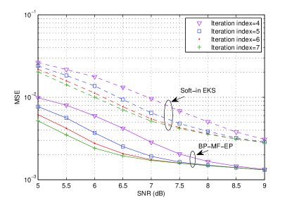
Figure 2: MSE performance of the phase noise estimation.

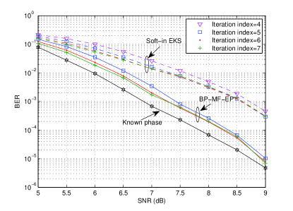
Figure 3: BER performance versus SNR.

We compare the MSE performance of the proposed algorithm with that of the Soft-in EKS algorithm for PN estimation. The results with different number of iterations are shown in Fig. 2. It can be seen that the proposed BP-MF-EP method significantly outperforms the Soft-in EKS method.

The comparisons of system BER performance are shown in Fig. 3, where the performance with known PN is also included for reference. It can be seen that considerable performance gains can be achieved by the proposed BP-MF-EP method compared to the Soft-in EKS method.

V CONCLUSIONS

In this paper we have proposed an iterative receiver for joint PN estimation, equalization and decoding based on combined BP, MF and EP. In particular, MF is used to tackle the factors due to the nonlinear observation model and the second-order Taylor expansion is used to achieve Gaussian approximation to the MF messages, which is crucial to the low complexity implementation of the receiver. The approximation is more effective than the direct local linearization of the observation model in the Soft-in EKS. As shown by the simulation results, the proposed method significantly outperforms the Soft-in EKS with similar complexity.

References

• [1] M. R. Khanzadi, D. Kuylenstierna, A. Panahi, T. Eriksson, and H. Zirath, “Calculation of the performance of communication systems from measured oscillator phase noise,” IEEE Trans. Circuits Syst. I, vol. 61, no. 5, pp. 1553 – 1565, May 2014.
• [2] J. Bhatti and M. Moeneclaey, “Iterative soft-decision-directed phase noise estimation from a DCT basis expansion,” in 2009 IEEE 20th International Symposium on Personal Indoor and Mobile Radio Communications, Sep. 2009, pp. 3228 – 3232.
• [3] F. Z. Merli and G. M. Vitetta, “A factor graph approach to the iterative detection of OFDM signals in the presence of carrier frequency offset and phase noise,” IEEE Trans. Wireless Commun., vol. 7, no. 3, pp. 868 – 877, Mar. 2008.
• [4] G. Colavolpe, A. Barbieri, and G. Caire, “Algorithms for iterative decoding in the presence of strong phase noise,” IEEE J. Select. Areas Commun., vol. 23, no. 9, pp. 1748 – 1757, Sep. 2005.
• [5] M. Nissilä and S. Pasupathy, “Adaptive iterative detectors for phase-uncertain channels via variational bounding,” IEEE Trans. Commun., vol. 57, no. 3, pp. 716 – 725, Mar. 2009.
• [6] M. Senst and G. Ascheid, “A combined belief propagation and mean field algorithm for soft carrier phase estimation,” 2011 8th International Symposium on Wireless Communication Systems, Aachen, 2011.
• [7] P. Sun, C. Zhang, Z. Wang, C. N. Manchón, and B. H. Fleury, “Iterative receiver design for ISI channels using combined belief- and expectationpropagation,” IEEE Signal Processing Lett., vol. 22, no. 10, pp. 1733 – 1737, Oct. 2015.
• [8] H. Mehrpouyan, A. A. Nasir, S. D. Blostein, T. Eriksson, G. K. Karagiannidis, and T. Svensson, “Joint estimation of channel and oscillator phase noise in MIMO systems,” IEEE Trans. Signal Processing, vol. 60, no. 9, pp. 4790 – 4807, Sep. 2012.
• [9] A. A. Nasir, H. Mehrpouyan, R. Schober, and Y. Hua, “Phase noise in MIMO systems: Bayesian Cramér-Rao bounds and soft-input estimation,” IEEE Trans. Signal Processing, vol. 61, no. 10, pp. 2675 – 2692, May 2013.
• [10] R. Krishnan, M. R. Khanzadi, L. Svensson, T. Eriksson, and T. Svensson, “Variational Bayesian framework for receiver design in the presence of phase noise in MIMO systems,” in 2012 IEEE Wireless Communications and Networking Conference (WCNC), Apr. 2012, pp. 347 – 352.
• [11] F. R. Kschischang, B. J. Frey, and H.-A. Loeliger, “Factor graphs and the sum-product algorithm,” IEEE Trans. Inform. Theory, vol. 47, no. 2, pp. 498 – 519, Feb. 2001.
• [12] J. Winn and C. M. Bishop, “Variational message passing,” Journal of Machine Learning Research, vol. 6, pp. 661 – 695, Dec. 2005.
• [13] G. Colavolpe, D. Fertonani, and A. Piemontese, “SISO detection over linear channels with linear complexity in the number of interferers,” IEEE Journal of selected topics in signal processing, vol. 5, no. 8, pp. 1475 – 1485, Dec. 2011.
• [14] R. Koetter, A. C. Singer, and M. Tücher, “Turbo equalization,” IEEE Signal Processing Mag., vol. 21, pp. 67 – 80, Jan. 2004.
• [15] E. Riegler, G. E. Kirkelund, C. N. Manchón, M.-A. Badiu, and B. H. Fleury, “Merging belief propagation and the mean field approximation: A free energy approach,” IEEE Trans. Inform. Theory, vol. 59, no. 1, pp. 588– 602, Jan. 2013.
• [16] M.-A. Badiu, G. E. Kirkelund, C. N. Manchón, E. Riegler, and B. H. Fleury, “Message-passing algorithms for channel estimation and decoding using approximate inference,” in IEEE Int. Symp. Inform. Theory (ISIT), Feb. 2012, pp. 2376 – 2380.
• [17] M. Badiu, C. N. Manchón, and B. H. Fleury, “Message-passing receiver architecture with reduced-complexity channel estimation,” IEEE Commun. Lett., vol. 17, no. 7, pp. 1404 – 1407, Jul. 2013.
• [18] C. Zhang, C. N. Manchón, Z. Wang, and B. H. Fleury, “Message-passing receivers for single carrier systems with frequency-domain equalization,” IEEE Signal Processing Lett., vol. 22, no. 4, pp. 404 – 407, Apr. 2015.
• [19] J. Hu, H.-A. Loeliger, J. Dauwels, and F. Kschischang, “A general computation rule for lossy summaries/messages with examples from equalization,” in Proc. 44th Allerton Conf. Communication, Control, and Computing, Sep. 2006, pp. 27 – 29.
• [20] Y. Qi and T. P. Minka, “Window-based expectation propagation for adaptive signal detection in flat-fading channels,” IEEE Trans. Commun., vol. 6, no. 1, pp. 348 – 355, Jan. 2007.
• [21] M. Nissilä and S. Pasupathy, “Joint estimation of carrier frequency offset and statistical parameters of the multipath fading channel,” IEEE Trans. Commun., vol. 54, no. 6, pp. 1038 – 1048, Jun. 2006.