Symmetry in Sphere-based Assembly Configuration Spaces

Abstract

Many remarkably robust, rapid and spontaneous self-assembly phenomena occurring in nature can be modeled geometrically, starting from a collection of rigid bunches of spheres. This paper highlights the role of symmetry in sphere-based assembly processes. Since spheres within bunches could be identical and bunches could be identical as well, the underlying symmetry groups could be of large order that grows with the number of participating spheres and bunches. Thus, understanding symmetries and associated isomorphism classes of microstates that correspond to various types of macrostates can significantly increase efficiency and accuracy, i.e., reduce the notorious complexity of computing entropy and free energy, as well as paths and kinetics, in high dimensional configuration spaces. In addition, a precise understanding of symmetries is crucial for giving provable guarantees of algorithmic accuracy and efficiency as well as accuracy vs. efficiency trade-offs in such computations. In particular, this may aid in predicting crucial assembly-driving interactions.

This is a primarily expository paper that develops a novel, original framework for dealing with symmetries in configuration spaces of assembling spheres, with the following goals. (1) We give new, formal definitions of various concepts relevant to the sphere-based assembly setting that occur in previous work, and in turn, formal definitions of their relevant symmetry groups leading to the main theorem concerning their symmetries. These previously developed concepts include, for example, (a) assembly configuration spaces, (b) stratification of assembly configuration space into configurational regions defined by active constraint graphs, (c) paths through the configurational regions, and (d) coarse assembly pathways. (2) We then demonstrate the new symmetry concepts to compute sizes and numbers of orbits in two example settings appearing in previous work. (3) Finally, we give formal statements of a variety of open problems and challenges using the new conceptual definitions.

1 Motivation

Supramolecular assembly is prevalent in nature, health-care and engineering, but poorly understood. The assembly starts with identical copies of structures drawn from a small number of types. Modeling these starting structures as rigid-bunches-of-spheres is well-suited to assembly processes driven by so-called short-range or hard sphere interaction potentials.

More formally, an input to a computational model of an assembly process is an assembly system consisting of the following.

• A collection of $k$ rigid molecular components belonging to a few types; a rigid component is specified as the set of positions of the centers of their constituent atoms, in a local coordinate system. In many cases, an atom could be the representation for the average position of a collection of atoms in an amino acid residue. Note that an assembly configuration is given by the positions and orientations of the entire set of $k$ rigid molecular components in an assembly system, relative to one fixed component. Since each rigid molecular component has six degrees of freedom, a configuration is a point in $6(k-1)$ dimensional Euclidean space.

• The pairwise component of the potential energy function of the assembly system, specified as a sum of potential energy terms between pairs of constituent atoms $i$ and $j$ in two different rigid components of the assembly system. The weak interaction between the rigid molecular components is captured by this potential energy function. The pairwise potential energy terms are, in turn, specified using pairwise potential energy functions similar to so-called Lennard-Jones potentials and Morse potentials [22]. The potential energy is a function of the distance $d_{i,j}$ between $i$ and $j$.

• A non-pairwise component of the potential energy function in the form of global potential energy terms that capture the tethers between the rigid components within a monomer, as well as other global potential energy terms that implicitly represent the solvent (water or lipid bilayer membrane) effect [47, 48, 36]. These are independent of particular pairs of atoms.

It is important to note that all the above potential energy terms are functions of the assembly configuration.

The formal conceptual framework we develop here is inspired by the following types of prediction questions.

• Input: the 3D descriptions of the rigid molecular components and their interactions (Section 2 describes how they are formally specified). Output: prediction of the final assembly structures and their likelihood.

• Input: as in the previous item, plus a 3D configuration of final assembled structure. Output: prediction of those interactions that are crucial for the assembly process to terminate in the given input assembly configuration.

• Input: as in the previous item. Output: prediction of minimal alterations of the building blocks or interactions that would significantly increase likelihood of the assembly process terminating in the given input assembly configuration.

• Input: as in the previous item, additionally more than one choice of final assembly configuration. Output: prediction of key events such as specific intermediate subassembly configuration choices during assembly that determine which one of the final assembly configuration is more likely to result.

Experimentally in vitro or vivo, these types of predictions about supramolecular assembly processes are difficult because of the remarkable rapidity, spontaneity and robustness of assembly processes. The prediction tasks highlight combinatorial explosion and thus insufficiency of experimentation (trying various possibilities) and guesswork, even with the help of known data on similar assemblies and biological knowledge about evolutionarily conserved structures. In addition, many of the current experimental methods are labor and resource-intensive, making blind alleys expensive in time and effort.

On the other hand, computer simulations guided by theoretical first principles and standard paradigms such as Monte Carlo(MC) or Molecular Dynamics(MD) are limited due to the reasons detailed in the next subsections.

1.1 Assembly Configurational Volume

Stability and binding affinity of subassemblies depend on free energy whose landscape in the case of assembly is heavily influenced by configurational entropy (volume measure of microstates corresponding to a macrostate; see [39]); this depends on accurate computation of configurational volumes by sampling, attempted by a long and distinguished series of methods [39, 3, 28, 29, 27, 43, 26, 63, 44]. Assembly configuration spaces are high dimensional, and the number of required samples is typically exponential in the dimension. Sampling on a high-dimensional ambient space grid typically means computing a large proportion of samples that lie outside any region of interest which is effectively of lower dimension, and these samples must be discarded. Not only are the relevant regions in the case of short-ranged potentials of effectively lower dimension, they are also geometrically/topologically complex, hence grid-based sampling in Cartesian space, as well as nonergodic methods like MC or MD, have to generate impractically dense sampling to accurately reflect the volume/measure ratios of these important, relatively low volume regions having complex geometry and topology. These methods do not exploit the abundance of symmetries of the landscape. They are used both for assembly processes, whose feasible regions are defined by one-sided pairwise distance equalities and inequalities between atom-centers, and folding processes, where the feasible regions are defined by pairwise distance equalities. The difference of complexity between the two is a litmus test for the limitations that are addressed by the Cayley configuration space approach taken by EASAL described in Section 1.5.

Conventional methods to compute the energy landscape of small clusters are based on searching for local minima [74, 21, 22]. Point group symmetrisation schemes [54, 77, 53] and local rigidification schemes [45, 62] have been exploited in global optimisation algorithms to gain computational efficiency.

Because of the complexity of the problem of dealing with the short range of interaction of hard spheres leading to narrow regions of lower potential energy, separated by vast flat parts, conventional local-minima based methods for energy landscape computation [74] are limited. These methods have the additional disadvantage of small perturbations to energy values requiring complete recomputation and also they do not deal well with the very flat landscape that is the signature of short-range potentials.

An alternative approach for short-range potentials is to consider the “sticky sphere limit” based on taking the limit as the range of interaction goes to zero [6, 70, 51]. In this limit, the energy landscape reduces to a collection of manifolds of different dimensions, glued together at their boundaries (formally, a Thom-Whitney stratification of real semi-algebraic sets), as described in theoretical models proposed independently and separately by Holmes-Cerfon et al. [33] in 2013 and by the first author’s research group [55, 56] in 2011.

The background provided in the remainder of this section recalls previously developed concepts for describing assembly configuration spaces. This motivates the conceptual framework for symmetry in assembly under short-ranged potentials given in Section 2.

1.2 Kinetics, Topology and Geometric complexity

Kinetics and transition rates between subassemblies also require an explicit understanding of the geometry, topology and multiple paths in the assembly configuration space. For cluster assemblies from spheres, there are a number of methods [4, 76, 8, 17, 42, 35, 34] to compute the entire configuration space of small molecules such as cyclo-octane [49, 37, 58]. Some methods from robotics and computational geometry [63], such as the probabilistic roadmap [2], effectively give bounds to approximate free energy without relying on MC or MD sampling. Starting from MC and MD samples, recent heuristic methods infer topology [23, 72, 46, 59], and use topology to guide dimensionality reduction [79]. Yet, most prevailing methods are unable to extract the topology in a sufficiently efficient and accurate manner as to be able to feasibly compute volume or path integrals (required for entropy or kinetics computations) even for small assemblies. Moreover even those prevailing methods that exploit symmetry in the configuration space to compute free energy and kinetics do not employ a formal and precise group-theoretic framework.

1.3 Recursive decomposition, Assembly trees, Combinatorial entropy

For larger, microscale assemblies, a direct study of the free energy and configurational entropy is computationally emphatically intractable. At these coarser scales, the primitives are stable subassemblies and transition rates (obtained from the computational tasks of the previous two subsections). Still, the combinatorial entropy of multiple pathways makes it difficult to isolate crucial combinations of assembly-driving interface interactions.

This issue has been addressed by the first author’s previous work on recursive decompositions [30, 31, 32] of larger assemblies into smaller subassemblies. This work introduces structures called assembly trees and the notion of combinatorial entropy, applied to model viral capsid assembly in [67].

While trees of various types have been used to model various processes related to assembly [18, 75], to the best of our knowledge, the assembly trees from [67] have a formal structure that is distinct from other tree representations of assembly pathways. In particular, non-root nodes of the assembly tree contain subassemblies, rather than configurations of the entire assembly system; and any pair of nodes that are incomparable (neither ancestor or child in the tree) are disjoint subassemblies, i.e, they do not contain any common rigid components; moreover, only rigid subassembly configurations are represented. In addition, the authors have taken the first steps towards precisely formalizing the effect of symmetries on a highly simplified version of assembly trees; specifically their orbits under the action of a fixed group of symmetries – called assembly pathways [13]. These concepts will be discussed in detail in Sections 2 and 3.

1.4 Symmetry in Chemistry

Since spheres within rigid bunches of an assembly system could be identical and bunches could be identical as well, the underlying symmetry groups could be of large order, that grows with the number of participating spheres and bunches. Therefore, all of the tasks in the previous three subsections can be significantly simplified by taking advantage of natural symmetries of the configuration space that arise due to identical assembling units, their symmetries, and symmetries of the final assembled structure. However, none of the prevailing methods discussed above computationally incorporates these symmetries. Group theory has been used to study the symmetry of molecules and molecular orbits  [16, 20, 14, 41] for a long time. The well-known Pólya enumeration theorem [57], which provides a method to find the number of orbits of a group action, is motivated by the problem of enumerating permutational isomers of a given molecular skeleton. Group theory is widely used in crystallography to describe crystallographic symmetry and classify crystal structures [1, 25]. Other applications include using the molecule symmetry group in studying molecular spectroscopy [15] and using generating functions in understanding nuclear spin statistics of nonrigid molecules [5]. However, most of these works only involve symmetry of individual structures. The literature is sparse in the context of symmetry in assembly systems or in configuration spaces.

1.5 EASAL: Efficient Atlasing and Search of Assembly Landscapes

A recent method of the first author, EASAL (efficient atlasing and search of assembly landscapes) [55, 56], formally addresses the issues highlighted in the first two subsections above: computation of configurational entropy and kinetics, via geometrization, stratification and convexification using Cayley parameterization of assembly configuration spaces. Geometrization and Stratification were also used later in [33] independently (as mentioned at the end of Section 1.1): the geometrization is achieved in [33] via a somewhat different process consistent with smooth potential energy functions, while the stratification is the standard Thom-Whitney stratification of semialgebraic sets as laid out in [55, 56].

On the other hand, Cayley convexification based on [68] is a unique feature of EASAL not present in [33], that makes it tractable to sample and compute entropy integrals over higher dimensional constant-potential-energy regions of the assembly configuration space. In addition Cayley convexification helps formalize and precisely explain the intuitively clear observation that assembly configuration spaces are significantly simpler geometrically and topologically than folding configuration spaces. The difference in complexity is especially stark when there are cycles of pairwise constraints between atom centers.

We describe the Geometrization and Stratification aspects of EASAL’s approach below. Stratification is explained in further detail in Section 2 and Cayley parameters for configuration spaces and convexification based on [68] are explained in Section 4.

1.5.1 Geometrization

The assembly configuration space is represented as a semi-algebraic set satisfying geometric constraints specified as distance inequalities between atom-centers. The short-range or hard sphere potential interaction is typically discretized to take different constant values on three intervals for the distance value $d_{i,j}$: $(0,r_{i,j})$, $(r_{i,j},r_{i,j}+\delta_{i,j})$, and $(r_{i,j}+\delta_{i,j},\infty).$ Typically, $r_{i,j}$, the so-called Van der Waal or steric radius, specifies ”forbidden” regions around atoms $i$ and $j.$ And $r_{i,j}+\delta_{i,j}$ is a distance where the attractive (electrostatic or other weak) forces between the two atoms is no longer strong (typically these forces decay as the reciprocal of some power of the distance $d_{i,j}$ between atom centers). Intuitively, the interval $(0,r_{i,j})$ is where the repulsive force highly dominates, and $(r_{i,j},r_{i,j}+\delta_{i,j})$ is where the attractive force and repulsive forces are balanced, and $(r_{i,j}+\delta_{i,j},\infty)$ is where neither force is strong. Over these 3 intervals respectively, the potential assumes a very high value, a very low value, and a medium value $m_{i,j}.$ All of these bounds for the intervals for $d_{i,j}$, as well as the values for the potential on these intervals, are specified as part of the input to the assembly model. These constants are specified for each pair of atoms $i$ and $j$, i.e., the subscripts are necessary. The interval with the low value is called the well. The Hard-Sphere potentials are defined solely by the Van der Waal’s forbidden distance constraint, $\delta_{i,j}=0$.

The information in the potential energy landscape can thus be geometrized, i.e., represented using assembly constraints, in the form of distance intervals. These constraints define feasible configurations. The set of feasible configurations is called the assembly configuration space. The active constraint regions of the configuration space are regions where at least one of the short-ranged inter-atom distances lies in the potential energy well, i.e, the interval $(r_{i,j},r_{i,j}+\delta_{i,j})$.

1.5.2 Stratification

The above geometrization of an assembly configuration space makes it natural to stratify an assembly configuration space into atlas of active constraint regions, More details are provided in Section 2 – see also Figure 7. The active constraint regions of the configuration space are regions where at least one of the inter-atom distances lies in the potential energy well. The active constraint regions are stratified by dimension into a topological Thom-Whitney complex, with the boundary region being one dimension smaller. The active constraint regions can be modeled as so-called convexifiable Cayley configuration spaces [68], a combinatorially definable concept by first labeling each region by its unique active constraint graph (see Section 2). A demo movie of EASAL is available at: http://www.cise.ufl.edu/research/SurfLab/EASALvideo.mpg. Standard algorithms can be employed for a fast computation of paths from one configuration to another in the atlas. However, the computation of entropy integrals over these paths poses several challenges.

1.6 Organization and Contribution

This is a primarily expository paper that develops a novel, original framework for dealing with symmetries in configuration spaces of assembling spheres under short ranged potentials. It is motivated by a longer-term goal to exploit natural symmetries using assembly trees and other concepts described in the previous sections, that have appeared in various avatars in the community, including our work on EASAL. Such an understanding of symmetries is essential for significantly reducing the complexity of the computation of configurational and combinatorial entropy as well as kinetics, since spheres within rigid bunches of an assembly system could be identical and bunches could be identical as well, giving underlying symmetry groups of large order, that grows with the number of participating spheres and bunches.

To this end, we develop a formal conceptual framework for assembly under short-ranged potentials, as assembly of rigid bunches of spheres. As different definitions of assembly macrostates are appropriate in different contexts, for example, depending on whether different copies of identical atoms or molecules are considered interchangeable or not, we carefully define and differentiate between congruence and isomorphism of configurations. We then show how symmetries of assembly configuration spaces arise due to: multiple copies of identical building blocks (in particular when these building blocks are rigid bunches of spheres), internal symmetries of building blocks, and the symmetries of the final assembled structure.

The organization of this paper is as following. In Section 2, we define the new conceptual framework for symmetry in assembly under short-ranged potentials (or assembly of rigid bunches of spheres) leading to the main Theorem 4. An application of some of these results on symmetry can be found in [56]. In Section 3, we illustrate one aspect of our approach [13] for computing combinatorial entropy using generating functions for counting the number and size of simplified assembly pathways (orbits of a symmetry group action on assembly trees). Note that while this simple example has a fixed group size, the method demonstrated applies also when the underlying symmetry group grows with the size of the system. In Section 4, open questions and directions are given.

2 Framework for Symmetry in Assembly

In this section, we define natural groups of symmetries acting on various previously defined objects related to symmetry that are described in the Introduction and later in this section. The four new groups we defined are the weak automorphism group, the strict congruence group, the strict order preserving isomorphism group and the strict permuted congruence group of an assembly configuration. We consider the action of these groups on various objects defined in previous literature on assembly and sketched in the introduction [55, 56, 66], such as assembly configuration space, active constraint regions, active constraint graphs, assembly paths and trees. These resulting symmetry classes will be used to formalize the main new Theorem 4 and two applications in Example 1 and Section 3, as well as open problems in the last section of this paper.

Let $X$ be a set under the action of a group $G$, and $x$ be any element of $X$. The orbit of $x$ under $G$ is the set $G(x)=\{\phi(x):\phi\in G\}$. An element $g$ of $G$ fixes $x$ if $g(x)=x$. The stabilizer subgroup $\mathit{stab}_{G}(x)$ of $x$ in $G$ is the group of all elements in $G$ that fix $x$, i.e.  $\mathit{stab}_{G}(x)=\{\phi\in G|\phi(x)=x\}$.

The following theorem from standard group theory can be used to determine the number of orbits and the size of orbits for various objects defined in this section. An explicit application of this theorem is shown in the next section.

Theorem 1.

Let $X$ be a set under the action of a group $G$. For all $x\in X$, the equalities

$$|G(x)|=|G|/|\mathit{stab}_{G}(x)|\qquad\text{(Orbit-Stabilizer theorem)}$$

and

$$|X/G|=\frac{1}{|G|}\sum_{\phi\in G}|X^{\phi}|\qquad\text{(Burnside's lemma)}$$

hold, where $|X/G|$ is the number of orbits of $X$, $X^{\phi}$ is the set $\{x\in X:\phi(x)=(x)\}$.

Different definitions of macrostates are appropriate in different contexts, for example, depending on whether different copies of identical atoms or molecules are considered interchangeable or not. For this reason we carefully define and differentiate between congruence and isomorphism of configurations.

In order to give a physically meaningful formalization of an assembly system under short-ranged potentials, we define the notion of a bunch, i.e., a rigid configuration of spheres of varying colors and radii.

2.1 A Bunch and its symmetries

Let $SE(3)$ denote the group of orientation preserving isometries of ${\mathbb{R}}^{3}$.

A bunch is a tuple $(P;\mathcal{C},r,\delta)$ where $P=(p_{1},p_{2},\ldots,p_{n})$ is an ordered set of points in ${\mathbb{R}}^{3}$, and $\mathcal{C},r,\delta$ are functions defining colored spheres centered at the points in $P$. Specifically, $\mathcal{C}:P\rightarrow C$ where $C$ is a finite set of “colors”, and $r,\delta:P\rightarrow{\mathbb{R}}^{+}$ such that the spheres are nonintersecting, i.e. $\|p_{i}-p_{j}\|_{2}\geq r(p_{i})+r(p_{j})$ for any $i\neq j$. The map $\delta$ is interpreted as the width of the annulus specified by the potential energy well and is used in the definition of an active constraint graph of an assembly configuration later in this section. For a bunch $B$, $P(B)$ is used to denote the point set $B$; similarly we have $\mathcal{C}(B),r(B)$ and $\delta(B)$.

Two bunches $B=(P;\mathcal{C},r,\delta)$ and $B^{\prime}=(P^{\prime};{\mathcal{C}}^{\prime},r^{\prime},\delta^{\prime})$ are isomorphic if there is an element $\phi$ of $SE(3)$ and a permutation $\pi\in S_{n}$, such that $\phi(p_{i})=p_{\pi(i)}^{\prime}$ for all $i$, where $n=|P|$, and $\phi$ preserves the color, radius and annulus of points. In this case with a slight abuse of notation, we write $B^{\prime}\in\phi(B)$, where $\phi(B)$ denotes the set of bunches that are isomorphic to $B$ under $\phi$ and some permutation in $S_{n}$. See Figure 1 for an example.

Two bunches $B=(P;\mathcal{C},r,\delta)$ and $B^{\prime}=(P^{\prime};{\mathcal{C}}^{\prime},r^{\prime},\delta^{\prime})$ are strictly isomorphic, if there is a permutation $\pi\in S_{n}$ such that $B$ and $B^{\prime}$ are isomorphic under $\pi$ and the identity element in $SE(3)$. The weak automorphism group of $B$, denoted $\mathit{Waut}(B)$, is the group of all permutations $\pi\in S_{n}$ that take $B$ to a strictly isomorphic $B^{\prime}$.

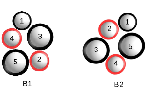
Figure 1: Two isomorphic bunches of 5 spheres

Two bunches $B=(P;\mathcal{C},r,\delta)$ and $B^{\prime}=(P^{\prime};{\mathcal{C}}^{\prime},r^{\prime},\delta^{\prime})$ are order preserving isomorphic or congruent, if there is a $\phi\in SE(3)$ such that $B$ and $B^{\prime}$ are isomorphic under $\phi$ and the identity permutation. In this case with a slight abuse of notation, we write $B^{\prime}=\phi(B)$.

We have the following observation that describes strict isomorphism using the notion of congruence.

Observation 2.

Two congruent bunches $B$ and $B^{\prime}$ are strictly isomorphic, if and only if $\tilde{P}=\tilde{P}^{\prime}$ where $\tilde{P}$ and $\tilde{P}^{\prime}$ denote the unordered point sets of $B$ and $B^{\prime}$ respectively, and for all $p\in P^{\prime}$, $\mathcal{C}^{\prime}(p)=\mathcal{C}(p)$, $r^{\prime}(p)=r(p)$, $\delta^{\prime}(p)=\delta(p)$.

2.2 An assembly configuration space and its symmetries

An assembly configuration is an ordered set $\mathcal{B}=(B_{1},B_{2}\ldots B_{k})$ where $B_{i}=(P_{i};\mathcal{C}_{i},r_{i},\delta_{i})$ is a bunch for all $i$, such that for all $i,j$ and all $x\in P_{i},\;y\in P_{j},\;x\neq y$, we have

$$\|x-y\|_{2}\geq r_{i}(x)+r_{j}(y)$$ (1 )

Two assembly configurations $\mathcal{B}=(B_{1},\ldots,B_{k})$ and $\mathcal{B}^{\prime}=(B_{1}^{\prime},\ldots,B_{k}^{\prime})$ are configurations of the same assembly system (see Section 1) if $B_{i}$ is congruent to $B_{\sigma(i)}^{\prime}$ for some permutation $\sigma\in S_{k}$, for all $i$. Notice that the congruence between bunches could be different for each $i$. The set of all assembly configurations of an assembly system is called an assembly configuration space. The assembly configuration space containing the assembly configuration $\mathcal{B}$ is denoted $\mathcal{A}(\mathcal{B})$, or simply $\mathcal{A}$ when the context is clear.

In the following discussion, we always restrict our universe to assembly configurations in the same assembly configuration space.

Two assembly configurations $\mathcal{B}=(B_{1},\ldots,B_{k})$ and $\mathcal{B}^{\prime}=(B_{1}^{\prime},\ldots,B_{k}^{\prime})$ are isomorphic if there is an element $\phi$ of $SE(3)$ (isomorphism between bunches) and a permutation $\sigma\in S_{k}$, such that for all $i$, $B_{\sigma(i)}^{\prime}$ is isomorphic to $B_{i}$ under $\phi$ and a permutation $\pi_{i}\in S_{n_{i}}$, where $n_{i}=|P_{i}|$.

Two assembly configurations $\mathcal{B}$ and $\mathcal{B}^{\prime}$ are strictly isomorphic, if there is a permutation $\sigma\in S_{k}$, such that for all $i$, $B_{\sigma(i)}^{\prime}$ is isomorphic to $B_{i}$ under the identity element in $SE(3)$ and a permutation $\pi_{i}\in S_{n_{i}}$, where $n_{i}=|P_{i}|$. Thus a strict isomorphism is a tuple of permutations $(\sigma,\pi_{1},\ldots,\pi_{k})$, where $\sigma\in S_{k}$ and $\pi_{i}\in S_{n_{i}}$. The weak automorphism group of $\mathcal{B}$, denoted $\mathit{Waut}(\mathcal{B})$, is the group of all such tuples $(\sigma,\pi_{1},\ldots,\pi_{k})$ that take $\mathcal{B}$ to a strictly isomorphic $\mathcal{B}^{\prime}$, with the group operation $(\sigma,\pi_{1},\ldots,\pi_{k})(\sigma^{\prime},\pi^{\prime}_{1},\ldots,\pi^{\prime}_{k})=(\sigma\sigma^{\prime},\pi_{1}\pi^{\prime}_{1},\ldots,\pi_{k}\pi^{\prime}_{k})$.

Note that all assembly configurations in the same assembly configuration space $\mathcal{A}$ have the same weak automorphism group. Thus we define the weak automorphism group of an assembly configuration space $\mathcal{A}$, denoted ${\mathit{Waut}\!_{\mathcal{A}}}$, to be the weak automorphism group of any assembly configuration $\mathcal{B}$ in $\mathcal{A}$.

Two assembly configurations $\mathcal{B}$ and $\mathcal{B}^{\prime}$ are congruent if there is an isomorphism $\phi\in SE(3)$ that preserves both the order of the bunches and the order of points within each bunch, i.e. for all $i$, $B_{i}^{\prime}$ is congruent to $B_{i}$ under $\phi$. Two assembly configurations $\mathcal{B}$ and $\mathcal{B}^{\prime}$ are strictly congruent if they are both congruent and strictly isomorphic. In general, we think of two strict congruent assembly configurations as the same. The strict congruence group of an assembly configuration $\mathcal{B}$ is the stabilizer of the set strictly congruent assembly configurations of $\mathcal{B}$ under ${\mathit{Waut}\!_{\mathcal{A}}}$. It is the stabilizer subgroup $\mathit{stab}_{{\mathit{Waut}\!_{\mathcal{A}}}}\mathcal{B}$ of the assembly configuration $\mathcal{B}$ under ${\mathit{Waut}\!_{\mathcal{A}}}$.

Two assembly configurations $\mathcal{B}$ and $\mathcal{B}^{\prime}$ are order preserving isomorphic if there is an isomorphism $\phi\in SE(3)$ that preserves the order of the bunches, i.e. for all $i$, $B_{i}^{\prime}$ is congruent to $\phi(B_{i})$. Two assembly configurations $\mathcal{B}$ and $\mathcal{B}^{\prime}$ are strictly order preserving isomorphic if they are both order preserving isomorphic and strictly isomorphic. The strict order preserving isomorphism group of an assembly configuration $\mathcal{B}$ is the stabilizer of the set of strictly order preserving isomorphic configurations of $\mathcal{B}$ under ${\mathit{Waut}\!_{\mathcal{A}}}$.

Two assembly configurations $\mathcal{B}$ and $\mathcal{B}^{\prime}$ are permuted-congruent if there is an isomorphism that preserves the order of points within each bunch, i.e. there is an element $\phi$ of $SE(3)$ and a permutation $\sigma\in S_{k}$, such that for all $i$, $B^{\prime}_{\sigma(i)}$ is congruent to $B_{i}$ under $\phi$. Two assembly configurations $\mathcal{B}$ and $\mathcal{B}^{\prime}$ are strictly permuted-congruent if they are both permuted-congruent and strictly isomorphic. The strict permuted congruence group of an assembly configuration $\mathcal{B}$ is the stabilizer of the set of permuted-congruent configurations of $\mathcal{B}$ under ${\mathit{Waut}\!_{\mathcal{A}}}$.

As an example, refer to Figure 2. The assembly configuration $\mathcal{B}_{1}$ consists of 3 congruent bunches. The assembly configuration $\mathcal{B}_{2}$ is obtained from $\mathcal{B}_{1}$ with a strict congruence $(\sigma,\pi_{1},\pi_{2},\pi_{3})$ induced by a rotation in $SE(3)$, where $\sigma=(1\;3)$, and $\pi_{i}=id$ for all $i$. The assembly configuration $\mathcal{B}_{3}$ is obtained from $\mathcal{B}_{1}$ with a strict permuted congruence $(\sigma,\pi_{1},\pi_{2},\pi_{3})$, where $\sigma$ is a cyclic permutation of the 3 bunches, and $\pi_{i}=id$ for all $i$. On the other hand, $\mathcal{B}_{4}$ is obtained from $\mathcal{B}_{1}$ with a strict isomorphism $(\sigma,\pi_{1},\pi_{2},\pi_{3})$, where $\sigma$ is a cyclic permutation of the 3 bunches, $\pi_{1}=(1\;2)$ and $\pi_{2}=\pi_{3}=id$.

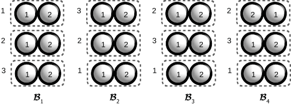
Figure 2: The assembly configuration $\mathcal{B}_{1}$ consists of 3 isomorphic bunches. $\mathcal{B}_{2}$ is obtained from $\mathcal{B}_{1}$ with a strict congruence, $\mathcal{B}_{3}$ is obtained from $\mathcal{B}_{1}$ with a strict permuted congruence, and $\mathcal{B}_{4}$ is obtained from $\mathcal{B}_{1}$ with a strict isomorphism that is neither a strict congruence, nor a strict permuted congruence, nor a strict order preserving isomorphism.

Figure 3 shows another example of four assembly configurations each containing two bunches. The strict congruence group $\mathit{stab}_{{\mathit{Waut}\!_{\mathcal{A}}}}\mathcal{B}$ of the assembly configuration $\mathcal{B}_{1}$ is of size 2 and contains those tuples $(\sigma,\pi_{1},\pi_{2})$, where $\pi_{1}\in\{id,(2\;4)\}$, $\sigma=id$, $\pi_{2}=id$. The weak automorphism group ${\mathit{Waut}\!_{\mathcal{A}}}$ of the assembly system is of size 4 and contains those tuples $(\sigma,\pi_{1},\pi_{2})$, where $\pi_{1}\in\{id,(2\;4),(3\;1),(2\;4)(3\;1)\}$, $\sigma=id$, $\pi_{2}=id$. All four strictly isomorphic assembly configurations are obtained by applying ${\mathit{Waut}\!_{\mathcal{A}}}$ to the assembly configuration $\mathcal{B}_{1}$. Notice that $\mathcal{B}_{2}$ and $\mathcal{B}_{1}$ ($\mathcal{B}_{4}$ and $\mathcal{B}_{3}$) are strictly congruent, while $\mathcal{B}_{3}$ and $\mathcal{B}_{1}$ are strictly order preserving isomorphic. The orbit of $\mathcal{B}_{1}$ under ${\mathit{Waut}\!_{\mathcal{A}}}$ is of size 2 and consists of $\mathcal{B}_{1}$ and $\mathcal{B}_{3}$.

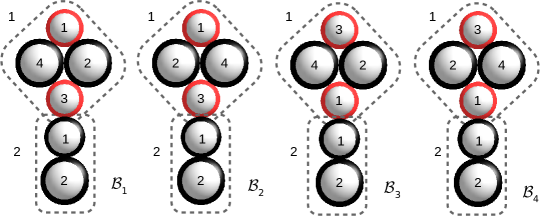
Figure 3: Four assembly configurations obtained by applying ${\mathit{Waut}\!_{\mathcal{A}}}$ on the assembly configuration $\mathcal{B}_{1}$. $\mathcal{B}_{2}$ is obtained from $\mathcal{B}_{1}$ with a congruence, while $\mathcal{B}_{3}$ is obtained from $\mathcal{B}_{1}$ with a strict order preserving isomorphism.

We have the following observations for alternative characterizations of strict congruence, strict order preserving isomorphism and strict permuted congruence of assembly configurations.

Observation 3.

Given two assembly configurations $\mathcal{B}=(B_{1},\ldots,B_{k})$ and $\mathcal{B}^{\prime}=(B_{1}^{\prime},\ldots,B_{k}^{\prime})$ in the same assembly configuration space,

1. $\mathcal{B}$ and $\mathcal{B}^{\prime}$ are strictly congruent if and only if they are congruent, and

   • $\mathcal{B}$ and $\mathcal{B}^{\prime}$ have the same unordered partition of the unordered point set into bunches, i.e. $\{\tilde{P_{1}},\ldots,\tilde{P_{k}}\}=\{\tilde{P^{\prime}_{1}},\ldots,\tilde{P^{\prime}_{k}}\}$, where $\tilde{P_{i}}$ is the unordered point set of the bunch $B_{i}$, and each point has same color, radius and annulus in $\mathcal{B}$ and $\mathcal{B}^{\prime}$.

2. $\mathcal{B}$ and $\mathcal{B}^{\prime}$ are strictly order preserving isomorphic if and only if they are order preserving isomorphic and satisfy the condition (*).

3. $\mathcal{B}$ and $\mathcal{B}^{\prime}$ are strictly permuted congruent if and only if they are permuted congruent and satisfy the condition (*).

2.3 Symmetries in active constraint graph and active constraint region

An active constraint graph $G(\mathcal{B})$ of an assembly configuration $\mathcal{B}=(B_{1},\ldots,B_{k})$ is a graph $(V,E)$, where the vertex set $V$ has one vertex for each point $p\in P_{1}\cup\ldots\cup P_{k}$, labeled by a tuple $(i,l)$, representing that the point $p$ appears as the $i^{th}$ point $p_{i}$ in the $l^{th}$ bunch $B_{l}$ of $\mathcal{B}$, and a vertex pair $\{x,y\}\in E$ if $x$ and $y$ lie in distinct bunches of $\mathcal{B}$ and

$$r(x)+r(y)\leq\|x-y\|_{2}\leq(r(x)+\delta(x))+(r(y)+\delta(y)).$$

An element $(\sigma,\pi_{1},\ldots,\pi_{k})$ of the weak automorphism group ${\mathit{Waut}\!_{\mathcal{A}}}$ of $\mathcal{B}$’s assembly configuration space $\mathcal{A}$ acts on $G(\mathcal{B})$ by taking the tuple $(i,l)$ to $(\pi_{l}(i),\sigma(l))$.

Two active constraint graphs $G_{1},G_{2}$ are isomorphic if there is a $\psi=(\sigma,\pi_{1},\ldots,\pi_{k})\in{\mathit{Waut}\!_{\mathcal{A}}}$ such that $\{x,y\}\in E(G_{1})\Longleftrightarrow\{\psi(x),\psi(y)\}\in E(G_{2})$. In this case we say $G_{1}\cong_{\psi}G_{2}$ or $\psi(G_{1})=G_{2}$.

The automorphism group of an active constraint graph $G$ is the group of elements $\psi\in{\mathit{Waut}\!_{\mathcal{A}}}$ such that $\psi(G)=G$, i.e. it is the stabilizer subgroup $\mathit{stab}_{\mathit{Waut}\!_{\mathcal{A}}}G$.

For example, Figure 4 shows all the non-isomorphic active constraint graphs with 12 edges of an assembly system consisting of 6 bunches, where all bunches are identical singleton spheres.

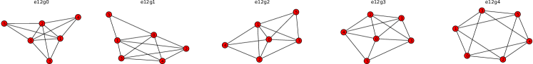
Figure 4: All non-isomorphic active constraint graphs with 12 edges of an assembly system of 6 bunches that are identical singleton spheres. The label on top is automatically generated by EASAL and specifies the orbit number of the shown active constraint graph.

Note: It is clear that $\mathit{stab}_{\mathit{Waut}\!_{\mathcal{A}}}{\mathcal{B}}\subseteq\mathit{stab}_{\mathit{Waut}\!_{\mathcal{A}}}G(\mathcal{B})$. Moreover, there are assembly configurations $\mathcal{B}$ such that $\mathit{stab}_{\mathit{Waut}\!_{\mathcal{A}}}{\mathcal{B}}\subsetneq\mathit{stab}_{\mathit{Waut}\!_{\mathcal{A}}}G(\mathcal{B})$, i.e. the strict congruence group of $\mathcal{B}$ does not have all the automorphisms of the corresponding active constraint graph. Refer to the assembly configuration $\mathcal{B}$ and its active constraint graph $G$ in Figure 5, where each bunch is a singleton sphere. The permutation $\sigma=(1\;2\;3)\in{\mathit{Waut}\!_{\mathcal{A}}}$ is contained in $\mathit{stab}_{\mathit{Waut}\!_{\mathcal{A}}}(G)$. However, it is not contained in the strict congruence group $\mathit{stab}_{\mathit{Waut}\!_{\mathcal{A}}}{\mathcal{B}}$ of the assembly configuration.

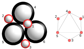
Figure 5: An assembly configuration whose automorphism group is strictly contained in that of the corresponding active constraint graph. Here the bunches are singleton spheres and bunches of the same color have the same $\mathcal{C}$, $r$ and $\delta$.

The full graph $G^{*}$ of an active constraint graph $G$ is obtained by adding edges to $G$ to make the set of vertices in each bunch into a clique.

An active constraint region $R_{G}$ of the assembly configuration space $\mathcal{A}$ contains all assembly configurations $\mathcal{B}$ with the active constraint graph $G(\mathcal{B})=G$. The action of elements of ${\mathit{Waut}\!_{\mathcal{A}}}$ on an active constraint region, and the stabilizer of an active constraint region in ${\mathit{Waut}\!_{\mathcal{A}}}$ are well-defined by the action of ${\mathit{Waut}\!_{\mathcal{A}}}$ on assembly configurations.

The following theorem gives containment and equality relations between stabilizer subgroups of an active constraint graph, an active constraint region and individual configurations in the active constraint region.

Theorem 4.

For an active constraint graph $G=G(\mathcal{B})$ of an assembly configuration space $\mathcal{A}$, it holds that

$$\mathit{stab}_{\mathit{Waut}\!_{\mathcal{A}}}{\mathcal{B}}\subseteq\mathit{stab}_{\mathit{Waut}\!_{\mathcal{A}}}G=\mathit{stab}_{\mathit{Waut}\!_{\mathcal{A}}}R_{G}$$

In addition, there exist active constraint graphs $G$ of assembly configuration spaces $\mathcal{A}$ where the above containment is strict, i.e.

$$\text{ for all }\mathcal{B}\text{ such that }G=G(\mathcal{B}),\quad\mathit{stab}_{\mathit{Waut}\!_{\mathcal{A}}}{\mathcal{B}}\subsetneq\mathit{stab}_{\mathit{Waut}\!_{\mathcal{A}}}G=\mathit{stab}_{\mathit{Waut}\!_{\mathcal{A}}}R_{G}$$

Proof.

(1) It is straightforward to see that $\mathit{stab}_{\mathit{Waut}\!_{\mathcal{A}}}{\mathcal{B}}\subseteq\mathit{stab}_{\mathit{Waut}\!_{\mathcal{A}}}G(\mathcal{B})$. We give an example to show the existence of $G$ where $\mathit{stab}_{\mathit{Waut}\!_{\mathcal{A}}}{\mathcal{B}}\subsetneq\mathit{stab}_{\mathit{Waut}\!_{\mathcal{A}}}G$ for any assembly configuration $\mathcal{B}$ of $G$. Refer to the assembly configuration in Figure 6, where each bunch is a singleton sphere. The permutation $\sigma=(1\;2\;3)$ is contained in the automorphism group $\mathit{stab}_{\mathit{Waut}\!_{\mathcal{A}}}G$ of the active constraint graph $G$. However, it is not contained in the strict congruence group of any corresponding assembly configuration, as the position of the sphere 6 is asymmetric with respect to $1,2,3$ in any assembly configuration of $G$. Thus $\mathit{stab}_{\mathit{Waut}\!_{\mathcal{A}}}{\mathcal{B}}\subsetneq\mathit{stab}_{\mathit{Waut}\!_{\mathcal{A}}}G$ for any assembly configuration $\mathcal{B}$ of $G$..

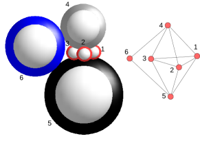
Figure 6: Any assembly configuration corresponding to the active constraint graph $G$ has its strict congruence group strictly contained in $\mathit{stab}_{\mathit{Waut}\!_{\mathcal{A}}}G$. Here the bunches are singleton spheres and bunches of the same color have the same $\mathcal{C}$, $r$ and $\delta$.

(2) $\mathit{stab}_{\mathit{Waut}\!_{\mathcal{A}}}G=\mathit{stab}_{\mathit{Waut}\!_{\mathcal{A}}}R_{G}$: from the definition of permutations in the weak automorphism group of the assembly configuration space, it follows that $\mathit{stab}_{\mathit{Waut}\!_{\mathcal{A}}}G\subseteq\mathit{stab}_{\mathit{Waut}\!_{\mathcal{A}}}R_{G}$. To show $\mathit{stab}_{\mathit{Waut}\!_{\mathcal{A}}}R_{G}\subseteq\mathit{stab}_{\mathit{Waut}\!_{\mathcal{A}}})$, consider any element $\psi\in\mathit{stab}_{\mathit{Waut}\!_{\mathcal{A}}}R_{G}$. For any assembly configuration $\mathcal{B}\in R_{G}$, if a pair of spheres $(x,y)$ are “touching” (i.e. they yield an edge in the corresponding active constraint graph), it must be the case that $(\psi(x),\psi(y))$ are also “touching” in $\psi(\mathcal{B})$, since $G(\mathcal{B})=G(\psi(\mathcal{B}))=G$. Similarly, $\psi$ must mapping “non-touching” pairs to “non-touching” pairs. Therefore $\psi\in\mathit{stab}_{\mathit{Waut}\!_{\mathcal{A}}}G$. ∎

Remark 1.

We expect the strict order preserving isomorphism group and the strict permuted congruence group of an assembly configuration $\mathcal{B}$ to lie between the strict congruence group $\mathit{stab}_{\mathit{Waut}\!_{\mathcal{A}}}\mathcal{B}$ and the automorphism group $\mathit{stab}_{\mathit{Waut}\!_{\mathcal{A}}}G$ of its active constraint graph. However, the containment relationship between these two groups is not clear.

2.4 Symmetries in stratification, assembly path and pathway

A stratification $\mathcal{S}(\mathcal{A})$ of the assembly configuration space $\mathcal{A}$ is a partition of the space into strata $\mathcal{X}_{i}$ of $\mathcal{A}$ that form a filtration $\emptyset\subset\mathcal{X}_{0}\subset\mathcal{X}_{1}\subset\ldots\subset\mathcal{X}_{m}=\mathcal{A}$, $m=6(n-1)$. Each $\mathcal{X}_{i}$ is a union of active constraint regions $R_{G}$, where the corresponding active constraint graph $G$ has $m-i$ independent edges, i.e. $m-i$ inequality constraints are active. Each active constraint graph $G$ is itself part of at least one, and possibly many, hence $l$-indexed, nested chains of the form $\emptyset\subset G^{l}_{0}\subset G^{l}_{1}\subset\ldots\subset G^{l}_{m-i}=G\subset\ldots\subset G^{l}_{m}$.

These induce corresponding reverse nested chains of active constraint regions $R_{G^{l}_{j}}$: $\emptyset\subset R_{G^{l}_{m}}\subset R_{G^{l}_{m-1}}\subset\ldots\subset R_{G^{l}_{m-i}}=R_{G}\subset\ldots R_{G^{l}_{0}}$. Note that here for all $l,j$, $R_{G^{l}_{m-j}}\subseteq\mathcal{X}_{j}$ is closed and $j$ dimensional. See Figure 7 for an example of assembly configuration space stratification.

Given two active constraint graphs $G_{i}$ and $G_{j}$, $R_{G_{i}}$ (resp. $G_{i}$) is a parent of $R_{G_{j}}$ (resp. $G_{j}$) (resp. $R_{G_{j}}$ is a child of $R_{G_{i}}$) if $G_{i}\subsetneq G_{j}$ and there does not exists an active constraint graph $G_{m}$ such that $G_{i}\subsetneq G_{m}\subsetneq G_{j}$. The parent-child relation provides a Hasse diagram of active constraint regions in the stratification of $\mathcal{A}$.

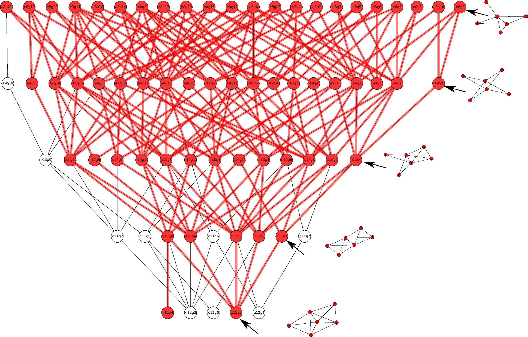
Figure 7: A fundamental region of the stratification for the assembly configuration space of the assembly configurations in Figure 4 of 6 bunches, with each bunch being a singleton sphere and all bunches identical. So ${\mathit{Waut}\!_{\mathcal{A}}}$ is the complete symmetric group of permutations of 6 elements, $S_{6}$. Each node shown is an orbit representative of an active constraint region corresponding to an active constraint graph. The grey part is those active constraint graphs (orbit representatives) whose corresponding constraint regions are empty. The example active constraint graph representatives on the right have arrows pointing to their regions in the stratification. The labels in the circles are unimportant: they are automatically generated and specify an orbit of an active constraint graph (example shown on right).

An assembly path from $G_{1}$ to $G_{m}$ in the stratification is a sequence $G_{1}\subsetneq G_{2}\subsetneq G_{3}\subsetneq\ldots\subsetneq G_{m}$ where $G_{i+1}$ is a child of $G_{i}$ for all $1\leq i\leq m$. A coarse assembly path from $G_{1}$ to $G_{m}$ in the stratification is a sequence $G_{1}\subsetneq G_{2}\subsetneq G_{3}\subsetneq\ldots\subsetneq G_{m}$ where $G^{*}_{i+1}$ has exactly one new rigid component $S$ not in $G^{*}_{i}$, with $S$ containing a set of two or more rigid components $S_{1}\ldots S_{m}$ of $G_{i}$. In addition, for all proper subsets $Q\subsetneq\{S_{1}\ldots S_{m}\}$ with $|Q|\geq 2$, the subgraphs of $G^{*}_{i+1}$ induced by $Q$ are not rigid. (The rigid components of a graph are the maximal rigid subgraphs. Two rigid components cannot intersect on more than two vertices. We refer the reader to combinatorial rigidity concepts in [24].)

For example, In Figure 7, the sequence of active constraint graphs on the right form an assembly path.

An assembly forest corresponding to a coarse assembly path from $G_{1}$ to $G_{m}$ is the unique forest where the leaves are the maximal rigid components of $G_{1}^{*}$. The internal nodes are the new rigid components $S$ occurring in some $G_{i+1}^{*}$ in the path. The children of $S$ are the set of rigid components $S_{1}\ldots S_{m}$ contained in $S$ that occur in $G_{i}^{*}$. The roots of the forest are the rigid components of $G_{m}^{*}$. An assembly tree is an assembly forest with only one root. See Figure 9 in Section 3 for examples of assembly trees [66, 13, 12].

A full (coarse) assembly path is an (coarse) assembly path from $G_{1}$ to $G_{m}$, where $G_{1}$ is the empty active constraint graph, and $G_{m}^{*}$ is a rigid active constraint graph. A (coarse) assembly path from primitives has the first property of the full assembly path, i.e. $G_{1}$ is the empty active constraint graph, but not the last property, i.e. $G_{m}$ can be any active constraint graph. The full assembly tree and assembly tree from primitives are also defined in this way.

A path between full active constraint graphs $G$ and $H$ where $G\nsubseteq H$ and $H\nsubseteq G$ is a sequence $G=G_{i},G_{i+1},G_{i+2},\ldots,G_{i+m}=H$, where any pair $G_{i+k}$ and $G_{i+k+1}$ are on some assembly path, and $G_{i+k}\subsetneq G_{i+k+1}$ if $k$ is even, $G_{i+k}\supsetneq G_{i+k+1}$ if $k$ is odd.

The fundamental domain of the stratification $\mathcal{S}(\mathcal{A})$ is the minimal sub stratification $\tilde{\mathcal{S}}(\mathcal{A})$ such that $\bigcup_{\pi\in{\mathit{Waut}\!_{\mathcal{A}}}}\pi(\tilde{\mathcal{S}}(\mathcal{A}))=\mathcal{S}(\mathcal{A})$, where $\pi$ acts on $\tilde{\mathcal{S}}(\mathcal{A})$ via its action on the active constraint regions (resp. active constraint graphs) of $\tilde{\mathcal{S}}(\mathcal{A})$. In other words the active constraint regions (resp. active constraint graphs) in $\tilde{\mathcal{S}}(\mathcal{A})$ are orbit representatives of active constraint regions (resp. active constraint graphs) under ${\mathit{Waut}\!_{\mathcal{A}}}$.

An assembly pathway is an orbit of an assembly tree under ${\mathit{Waut}\!_{\mathcal{A}}}$. The definition extends to full, and coarse assembly trees.

2.5 Example illustrating above symmetries

Some of the symmetry concepts defined here were used in [56] to efficiently compute path and higher dimensional region intervals in sphere-based assembly configuration spaces more efficiently reproducing and extending the results in [33]. We give a brief description here in the form of an example:

Example 1.

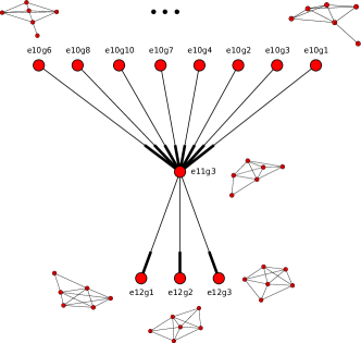
Figure 8: The neighbors of one active constraint graph in the Hasse diagram of the stratification for the assembly system in Figure 4

As an example, Figure 7 shows the Hasse diagram of the fundamental region of a stratification of an assembly system of 6 bunches that are identical singleton spheres considered first in [33]. Figure 8 shows an (orbit representative of an) active constraint graph of the system together with its parents and children in the Hasse diagram.

In addition, orbit representatives of paths help in improving efficiency of path integrals. in Figure 7, any path that goes down from the top of the diagram to the bottom is the orbit representative of an assembly path. In Figure 8, the sequence $e10q6\subsetneq e11g3\subsetneq e12g2$ is the orbit representative of an assembly path but not a coarse assembly path, as none of $e11g3$’s rigid components contains two or more rigid components of $e10g6$. On the other hand, the sequence $e10q6\subsetneq e12g2$ is the orbit representative of a coarse assembly path.

3 Enumerating Simple Assembly Pathways

In this section, we consider the action of the strict congruence group of a single final configuration on its assembly trees, and use generating functions to count the number and sizes of simplified assembly pathways [13]. Note that our approach could potentially be applied for all other groups defined in Section 2, the largest of which is the weak automorphism group of the final configuration, which would be the same as the weak automorphism group of the assembly configuration space.

A simple assembly is modeled by a rooted tree, the leaves are abstract representation of individual bunches, the root representing the final assembled configuration. The internal vertices represent intermediate stages of assembly, simplified to be subsets instead of subgraphs of the root. This simplification results in a loss of information about the assembly configuration space and active constraint graphs of the intermediate stages of assembly. To compensate, the group is taken to be the automorphism group $G$ of the graph of the assembled structure at the root instead of the weak automorphism group ${\mathit{Waut}\!_{\mathcal{A}}}$ of the assembly configuration space.

The definitions of assembly tree and pathway are simplified as follows. Given a finite group $G$ acting on a finite set $X$, we will define a simplified assembly pathway for the pair $(G,X)$. First, a simplified assembly tree is a rooted tree for which each internal vertex has at least two children and whose leaves are bijectively labeled with elements of a set $X$. There is an induced labeling on all the vertices of a simplified assembly tree by labeling a vertex $v$ by the set of labels on the leaves that are descendents of $v$. We identify each vertex of a simplified assembly tree with its label. Two simplified assembly trees are considered identical if there is a root preserving, adjacency preserving, and label preserving bijection between their vertex sets. The $26$ simplified assembly trees with four leaves, labeled in the set $X=\{1,2,3,4\}$ are shown in Figure 9.

For a simplified assembly tree $\tau$, the action of $G$ on $X$ induces a natural action of $G$ on the power set of $X$ and thereby on the set of vertices of $\tau$. Let $\mathcal{T}_{X}$ denote the set of all simplified assembly trees for $X$. If $g\in G$, then define the tree $g(\tau)$ as the unique simplified assembly tree whose set of vertex labels (including the labels of internal vertices) is $\{g(v):v\in\tau\}$. Thus we have an induced action of $G$ on $\mathcal{T}_{X}$. Each orbit of this action of $G$ on ${\mathcal{T}}_{X}$ consists of a set of simplified assembly trees called a simplified assembly pathway for $(G,X)$.

Figure 9: Klein 4-group acting on $\mathcal{T}_{4}$.

Example 2 (Klein 4-group acting on $\mathcal{T}_{4}$).

Consider the Klein 4-group $G={\mathbb{Z}}_{2}\oplus{\mathbb{Z}}_{2}$ acting on the set $X=\{1,2,3,4\}$. Writing $G$ as a group of permutations in cycle notation, this action is

$$G=\{(1)(2)(3)(4),\,(1\;2)(3\;4),\,(1\;3)(2\;4),\,(1\;4)(2\;3)\}.$$

For this example there are exactly 11 simplified assembly pathways, which are indicated in Figure 9 by boxes around the orbits. There are four simplified assembly pathways of size one, i.e., with one simplified assembly tree in the orbit, three simplified assembly pathways of size two, and four simplified assembly pathways of size four.

For any subgroup $H$ of $G$, let $t_{X}(H)$ denote the number of trees in $\mathcal{T}_{X}$ that are fixed by every element of $H$. Furthermore, let $\overline{t}(H):=\overline{t_{X}}(H)$ denote the number of trees in $\mathcal{T}_{X}$ that are fixed by every element of $H$ but by no other elements of $G$. In other words,

$$\overline{t}_{X}(H)=|\{\tau\in\mathcal{T}_{X}\,|\,stab_{G}(\tau)=H\}|.$$ (2 )

The first theorem below reduces the enumeration of simplified assembly pathways to the calculation of $\overline{t}(H)$ for subgroups $H$ of $G$. The index of a subgroup $H$ in $G$, i.e. the number of left (equivalently, right), cosets of $H$ in $G$ is denoted by $(G:H)$. By Lagrange’s Theorem, this index equals $|G|/|H|$. The second theorem below reduces the calculation of $\overline{t}(H)$ to the calculation of $t(H)$. The desired quantities $\overline{t}_{X}(H)$ are computed from the numbers $t_{X}(H)$ using Möbius inversion on the lattice of subgroups of $G$.

Theorem 5.

The number of trees in any simplified assembly pathway for $(G,X)$ divides $|G|$. If $m$ divides $|G|$, then the number $N(m)$ of simplified assembly pathways of cardinality $m$ is

$$N(m)=\frac{1}{m}\;\sum_{H\leq G\,:\,(G:H)=m}\;\overline{t}(H).$$

Theorem 6.

Let $G$ be a group acting on a set $X$. If $H$ is a subgroup of $G$, then

$$\overline{t_{X}}(H)=\sum_{H\leq K\leq G}\;\mu(H,K)\;t_{X}(K),$$

where $\mu$ is the Möbius function for the lattice of subgroups of $G$.

Example 3 (Klein 4-group acting on ${\mathcal{T}}_{4}$ - continued).

Theorem 5, applied to our previous example of ${\mathbb{Z}}_{2}\oplus{\mathbb{Z}}_{2}$ acting simply on $\{1,2,3,4\}$, states that the size of a simplified assembly pathway must be $1$, $2$ or $4$, since it must be a divisor of $4=|{\mathbb{Z}}_{2}\oplus{\mathbb{Z}}_{2}|$. To find the number of pathways of each size, note that $G$ has three subgroups of order 2, namely

$$K_{1} =\{\,(1)(2)(3)(4),(1\;2)(3\;4)\,\},$$

$$K_{2} =\{\,(1)(2)(3)(4),(1\;3)(2\;4)\,\},$$

$$K_{3} =\{\,(1)(2)(3)(4),(1\;4)(2\;3)\,\},$$

and that

$$\overline{t}(G)=4,$$

$$\overline{t}(K_{1})=\overline{t}(K_{2})=\overline{t}(K_{3})=2,$$

$$\overline{t}(K_{0})=16,$$

where $K_{0}$ denotes the trivial subgroup of order 1. The simplified assembly trees in ${\mathcal{T}}_{X}$ that are fixed by all elements of $G$ are shown in Figure 9, $A,B,C,D$. For $i=1,2,3$, those simplified assembly trees in ${\mathcal{T}}_{X}$ that are fixed by all elements of $K_{i}$ and by no other elements of $G$ are are shown in Figure 9, $E,F,G$, respectively. The remaining 16 simplified assembly trees in Figure 9 are fixed by no elements of $G$ except the identity. Therefore, according to Theorem 5, the number of pathways of size 1, 2 and 4 are, respectively,

$$\overline{t}(G) =4,$$

$$\frac{1}{2}\,\left(\,\overline{t}(K_{1})+\overline{t}(K_{2})+\overline{t}(K_{3})\,\right)=\frac{1}{2}\,(2+2+2) =3,$$

$$\frac{1}{4}\,\overline{t}(K_{0}) =4.$$

The problem of enumerating simplified assembly pathways is reduced, using Theorems 5 and 6, to calculating the number $t(G)$ of simplified assembly trees fixed by a given group $G$. This is done using permutation group theory and generating functions. It will be assumed, as is the case in many of the biological appllications, that $G$ acts freely on $X$, i.e., if $g(x)=x$ for some $x\in X$, then $g$ must be the identity. In this case

$$|X|:=|X_{n}|=n\cdot|G|,$$

where $n$ is the number of $G$-orbits in its action on $X$. Denote by $t_{n}(G)$ the number of trees in ${\mathcal{T}}_{n}:={\mathcal{T}}_{X_{n}}$ that are fixed by $G$. We define the exponential generating function

$$f_{G}(x):=\sum_{n\geq 1}t_{n}(G)\,\frac{x^{n}}{n!}$$

for the sequence $\{t_{n}(G)\}$.

If $G$ is the trivial group of order one, then let us denote this generating function simply by $f(x)$. This is the generating function for the total number of rooted, labeled trees with $n$ leaves in which every non-leaf vertex has at least two children. For $H\leq G$, let

$$\widehat{f}_{H}(x)=\frac{1}{(G:H)}\;f_{H}\left((G:H)x\right).$$

Theorem 7.

The generating function $f_{G}(x)$ satisfies the following functional equations:

$$1-x+2f(x)=\exp\,(f(x)),$$

and for $|G|>1$,

$$1+2f_{G}(x)=\exp\,\left(\sum_{H\leq G}\;\widehat{f}_{H}(x)\right).$$

Althogh proofs are omitted in this survey, the rather involved proof of Theorem 7 relies on, in addition to generating function techniques, a characterization of block systems arising from a group acting on a set and a recursive procedure for constructing all trees in $\mathcal{T}_{X}$ that are fixed by $G$. (See [13, Theorems 9 and 14].)

Remark 2.

Finding the generating function $f_{G}(x)$ depends on first finding the generating functions $f_{H}(x)$ for proper subgroups $H$ of $G$. In that sense, the procedure for finding $f_{G}(x)$ is recursive, proceeding up the lattice of subgroups of $G$, starting from the trivial subgroup.

It is also worth mentioning that subgroups that are conjugate in $G$ have the same generating function.

Example 4 (Klein 4-group acting on ${\mathcal{T}}_{4}$ - continued).

Consider $G={\mathbb{Z}}_{2}\oplus{\mathbb{Z}}_{2}$ acting on $X_{n}$. Recall that $|X_{n}|=4n$, the integer $n$ being the number of $G$-orbits. Recall that the subgroups of $G$ are $K_{0},K_{1},K_{2},K_{3},G$, where $K_{0}$ is the trivial group and

$$K_{1} =\{\,(1)(2)(3)(4),(1\;2)(3\;4)\,\},$$

$$K_{2} =\{\,(1)(2)(3)(4),(1\;3)(2\;4)\,\},$$

$$K_{3} =\{\,(1)(2)(3)(4),(1\;4)(2\;3)\,\}.$$

The functional equations in the statement of Theorem 7 are

$$1-x+2f(x) =\,\exp\,(f(x))$$

$$1+2f_{K_{i}}(x) =\,\exp\,\left(\frac{1}{2}\,f(2x)+f_{K_{i}}(x)\right)\quad\text{for $i=1,2,3$, and}$$

$$1+2f_{G}(x) =\,\exp\,\left(\frac{1}{4}\,f(4x)+\frac{1}{2}\,f_{K_{1}}(2x)+\frac{1}{2}\,f_{K_{2}}(2x)+\frac{1}{2}\,f_{K_{3}}(2x)+f_{G}(x)\right).$$

Using these equations and MAPLE software, the coefficients of the respective generating functions provide the following first few values for the number of fixed simplified assembly trees. For the first entry $t_{1}(G)=4$ for the group $G$, the four fixed trees are shown in Figure 9 $A$, $B$, $C$, $D$. For trees with eight leaves there are $t_{2}(G)=104$ simplified assembly trees fixed by $G={\mathbb{Z}}_{2}\oplus{\mathbb{Z}}_{2}$, and so on.

$$t_{n}(K_{0}) :\quad 1,1,4,26,236,2752$$

$$t_{n}(K_{i}) :\quad 1,6,72,1312,32128,989696$$

$$t_{n}(G) :\quad 4,104,4896,341120,31945728,3790876672.$$

Example 5 (The icosahedral group acting on a viral capsid).

A symmetry of a polyhedron is a transformation in SE$(3)$ that keeps the polyhedron, as a whole, fixed, and a direct symmetry is similarly defined. The icosahedral group is the group of direct symmetries of the icosahedron. It is a group of order 60 denoted $G_{60}$.

A viral capsid assembly configuration is modeled by a polyhedron $P$ with icosahedral symmetry. Its set $X$ of facets represent the protein monomers. The icosahedral group acts on $P$ and hence on the set $X$. It follows from the so-called quasi-equivalence theory of the capsid structure that $G_{60}$ acts freely on $X$. We have $|X|:=|X_{n}|=60n$, where $n$ is the number of orbits in the action of the icosahedral group on $X$. Not every $n$ is possible for a viral capsid; $n$ must be a $T$-number, that is, a number of form $h^{2}+hk+k^{2}$, where $h$ and $k$ are nonnegative integers.

Note. An icosahedral viral capsid assemly configuration has a corresponding icosahedral active constraint graph. And the group $G_{60}$, viewed as a subgroup of the symmetric group $S_{60}$ is the automorphism group of this active constraint graph. As mentioned in the beginning of this section, we are interested in the orbits of simplified assembly trees under the action of this automorphism group. However, we continue to use the more intuitive view of $G_{60}$ as a geometric group.

Before the number of simplified assembly trees can be enumerated, basic information about the icosahedral group is needed. The group $G_{60}$ consists of:

• the identity,

• 15 rotations of order 2 about axes that pass through the midpoints of pairs of diametrically opposite edges of $P$,

• 20 rotations of order 3 about axes that pass through the centers of diametrically opposite triangular faces, and

• 24 rotations of order 5 about axes that pass through diametrically opposite vertices.

There are 59 subgroups of $G_{60}$ that play a crucial role in the theory. Besides the two trivial subgroups, they are the following:

• 15 subgroups of order 2, each generated by one of the rotations of order 2,

• 10 subgroups of order 3, each generated by one of the rotations of order 3,

• 5 subgroups of order 4, each generated by rotations of order 2 about perpendicular axes,

• 6 subgroups of order 5, each generated by one of the rotations of order 5,

• 10 subgroups of order 6, each generated by a rotation of order 3 about an axis L and a rotation of order 2 that reverses L,

• 6 subgroups of order 10, each generated by a rotation of order 5 about an axis L and a rotation of order 2 that reverses L,

• 5 subgroups of order 12, each the symmetry group of a regular tetrahedron inscribed in $P$.

From the above geometric description of the subgroups, it follows that all subgroups of a given order are conjugate in the group $G_{60}$. Representatives of the conjugacy classes of the subgroups of the icosahedral group are denoted by $G_{0},G_{2},G_{3},G_{5},G_{6},G_{10},G_{12},G_{60}$, where the subscript is the order of the group. The set of subgroups of $G_{60}$ forms a lattice, ordered by inclusion. A partial Hasse diagram for this lattice $\bf L$ is shown in Figure 10. The number on the edge joining $G_{i}$ (below) and $G_{j}$ (above) indicate the number of distinct subgroups of order $i$ contained in each subgroup of order $j$. The number in parentheses on the edge joining $G_{i}$ (below) and $G_{j}$ (above) indicate the number of distinct subgroups of order $j$ containing each subgroup of order $i$. The Möbius function of $\bf L$ is shown in Table 1. The entry in the table corresponding to the row labeled $G_{i}$ and column $G_{j}$ is $\mu(G_{i},G_{j})$.

Figure 10: Partial Hasse diagram for the lattice of subgroups of the icosahedral group.

Table 1: The values of the Möbius function of the subgroup lattice of $G_{60}$.

Consider the case $|X|=60$, i.e., for the $T=1$ capsid. Using Theorem 7 and MAPLE software, the generating functions $f_{G_{i}}(x)$ were computed, and hence their coefficients $t_{60/i}(G_{i})$ which count simplified assembly trees that are fixed by any copy of $G_{i}$ were also computed. Note that, since $|X|=60$, the number of orbits of $G_{i}$ in its action on $X$ is $60/i$. Substituting these values into Theorem 6 and using the Möbius Table 1 yields the numerical values for $\overline{t}_{60/i}(G_{i})$, the number of simplified assembly trees over $X$ with $|X|=60$ that are fixed by $G_{i}$ but by no other elements of $G_{60}$. In other words, these are the numbers of trees whose stabilizer in $G_{60}$ is exactly $G_{i}$. Substituting these numbers $\overline{t}$ into Theorem 5, we arrive at the number of simplified assembly pathways of each possible size:

$$\begin{array}[]{ll}204&\text{simplified assembly pathways of size $1$}\\ \sim$168\text{\times}{10}^{8}$&\text{simplified assembly pathways of size $5$}\\ \sim$223\text{\times}{10}^{9}$&\text{simplified assembly pathways of size $6$}\\ \sim$613\text{\times}{10}^{17}$&\text{simplified assembly pathways of size $10$}\\ \sim$102\text{\times}{10}^{17}$&\text{simplified assembly pathways of size $12$}\\ \sim$334\text{\times}{10}^{28}$&\text{simplified assembly pathways of size $15$}\\ \sim$504\text{\times}{10}^{31}$&\text{simplified assembly pathways of size $20$}\\ \sim$835\text{\times}{10}^{51}$&\text{simplified assembly pathways of size $30$}\\ \sim$320\text{\times}{10}^{99}$&\text{simplified assembly pathways of size $60$}\end{array}$$

4 Open Questions

4.1 Enumeration problems in (non-simplified) assembly framework

We are interested in the following enumeration problems related to the action of ${\mathit{Waut}\!_{\mathcal{A}}}$ for the framework in Section 2:

1. How to compute the size of orbits/stabilizers and the number of orbits under ${\mathit{Waut}\!_{\mathcal{A}}}$ for assembly configurations, active constraint graphs, active constraint regions, (coarse) assembly paths and assembly trees/forests?

2. How to compute the number of coarse assembly paths that correspond to a particular assembly tree/forest?

3. Given two active constraint graphs $G$ and $H$, where $G$ and $H$ are incomparable, i.e. $G\nsubseteq H$ and $H\nsubseteq G$, how to compute the number of paths between them?

4. Given two active constraint graphs $G_{1}$ and $G_{m}$, where $G_{1}\subsetneq G_{m}$, how to compute the number of (coarse) assembly paths from $G_{1}$ to $G_{m}$?

5. What are the orbits of the (coarse) assembly paths in (4) under the action of $\mathit{stab}_{\mathit{Waut}\!_{\mathcal{A}}}(G_{m})$?

6. What are the orbits of the (coarse) assembly paths in (4) under the action of the group $H$, where $H={\mathit{Waut}\!_{\mathcal{A}}}$ if $\mathit{stab}_{\mathit{Waut}\!_{\mathcal{A}}}(G_{1})={\mathit{Waut}\!_{\mathcal{A}}}$ (i.e. $G_{1}$ is the empty active constraint graph), or $H=\mathit{stab}_{\mathit{Waut}\!_{\mathcal{A}}}(G_{1})\cap\mathit{stab}_{\mathit{Waut}\!_{\mathcal{A}}}(G_{m})$ otherwise?

4.2 Symmetries within an active constraint region via Cayley configurations

So far, we have discussed the orbit of an active constraint region and active constraint graph, and pointed out that it is sufficient to deal with a single orbit representative provided we are able to compute the multiplying factors associated with the size of the orbit, stabilizer, number of orbits etc.

In fact, a single active constraint region could be decomposed into the union of nontrivial subregions that form the orbit of a fundamental region, leading to enormous efficiencies in sampling, computation of volumes that are currently hoplessly intractable in high dimensional configuration spaces as discussed in the Introduction.

In fact since the fundamental region itself could have subregions with varying orders of stabilizers, we could decompose into more than one orbit representative, with different stabilizers. In any case, sampling or computing the volume of an active constraint region is simplified by sampling these fundamental subregions and computing the size of their orbits.

One way to obtain such a decomposition of an active constraint region $R_{G}$ is via the locally complete Cayley (assembly) configurations $\delta_{F}$ corresponding to the active constraint graph $G$. Convex Cayley configuration spaces highlight the key difference between assembly and other constraint systems e.g., folding. This difference is captured in the combinatorial structure of active constraint graphs. A Cayley parameter for an active constraint region $R_{G}$ is a non-edge of its active constraint graph $G$. For specific sets of non-edges $F$, the set of vectors $\lambda_{F}$ of attainable lengths of $F$ - (in 3D realizations of a linkage $(G,\delta)$ with underlying graph $G$ and edge lengths $\delta$) - is always convex for any given lengths $\delta$ (that is, for all the 3D realizations of the bar-joint constraint system or linkage $(G,\delta)$). This set is called the (3-dimensional) Cayley configuration space of the linkage $(G,\delta)$ on the Cayley parameters $F$, denoted $\Phi_{F}(G,\delta)$ and can be viewed as a “projection” of the space of pairwise distance vectors of realizations of $(G,\delta)$ on the Cayley parameters $F$. Such graphs $G$ are said to have convexifiable Cayley configuration spaces with parameters $F$ (short: convexifiable). Convexity permits the use of convex programming techniques for improving efficiency of sampling, search, volume computations etc. for the configuration space.

The concept is best explained using key theorems of the first author in [68, 69] discussed in Section 4.

We assume knowledge of common graph operations such as $k$-sums and resulting partial $k$-trees, a minor-closed class (partial 2-trees are series-parallel graphs with a forbidden minor $K_{4}$).

Theorem 8.

[68] A graph $H$ has a convexifiable Cayley configuration space with parameters $F$ if and only if for each $f\in F$ all the minimal 2-sum components of $H\cup F$ that contain both endpoints of $f$ are partial 2-trees. The Cayley configuration space $\Phi_{F}(H,\delta)$ of a bar-joint system or linkage $(H,\delta)$ is a convex polytope. When $H\cup F$ is a 2-tree, the bounding hyperplanes of this polytope are triangle inequalities relating the lengths of edges of the triangles in $H\cup F$.

Note: A major advantage of the convex Cayley method is that sampling the configuration space can be effected by standard methods of convex programming. Another advantage is that the method is completely unaffected when $\delta$ are intervals rather than exact values  [68]. A different characterization of inherent Cayley convexity for a graph $G$ on a set $F$ of non-edges as in the above section has been proven also for higher dimensions $d$ [68], [19], showing equivalence to a minor-closed property of $d$-flattenability introduced in [7] and also for other, non-euclidean distances (norms) in [69]. Any realization of $H$ in a normed space can be flattened into $d$-dimensional normed space (in the same norm) maintaining the same edge distances.

Theorem 9.

[69] A graph $H$ is $d$-flattenable if and only if for every partition of $H$ into $G\cup F$, $G$ has a convex Cayley configuration space on $F$ in $d$-dimensions.

4.2.1 Fundamental regions of Active constraint regions

After $G$ has been completed with the convexifying Cayley parameters $F$, the locally rigid graph $G\cup F$ typically loses symmetries present in $G$, i.e, the automorphism group is smaller. However, $F$ can be replaced by any set of edges $\pi(F)$ for $\pi\in\mathit{stab}_{\mathit{Waut}\!_{\mathcal{A}}}(G)$. Each locally complete Cayley configuration in the active constraint region $G$ is of the form $\delta_{F}$ (lengths of edges in $F$, where $G\cup F$ is rigid). Each cartesian (assembly) configuration within an active constraint region with graph $G$ corresponds bijectively to a globally complete Cayley configuration $(\delta_{F},\delta_{H})$ where $G\cup F$ is rigid and $G\cup F\cup H$ is globally rigid (or even $G\cup F\cup H$ is complete graph).

Thus when sampling the Cayley configuration space on $F$, one can find the boundaries of the fundamental regions corresponding to the corresponding cartesian assembly configurations as follows. For a Cayley configuration $\delta_{F}$, all its generically finitely many real/cartesian configurations can be obtained as various corresponding values of $\delta_{H}$, which include the values of $\delta_{\pi(F)}$. The boundary of a fundamental region occurs during sampling when we encounter a cartesian (assembly) configuration $c$ where the lengths of $\pi(F)$ correspond to already sampled lengths of $F$.

Note that there could be a different decomposition into fundamental regions, corresponding to each cartesian configuration (type) corresponding to the Cayley configuration. For example, for a different configuration $c^{\prime}$ from the configuration $c$ above, the lengths of $\pi(F)$ may not correspond to already sampled lengths of $F$. Or, there could be another element $\sigma\in\mathit{stab}_{\mathit{Waut}\!_{\mathcal{A}}}(G)$, with $\sigma\neq\pi$ where the lengths of $\sigma(F)$ in $c^{\prime}$ could correspond to already sampled lengths of $F$. In this manner, one can, in principle, algorithmically bound fundamental regions $R^{i}_{G}$ of the active constraint region $R_{G}$, by inspecting the assembly configurations corresponding to the Cayley configuration space on $F$, such that the active constraint region $R_{G}$ is the union of the orbits of the regions $R^{i}_{G}$ (under the action of $\mathit{stab}_{\mathit{Waut}\!_{\mathcal{A}}}(G)$).

Efficiently finding these fundamental regions as well as the number and sizes of their orbits is an open question, whose answer would enormously reduce the complexity of configurational entropy computations for assembly.

4.3 $g$-unfixable unlabeled trees

Call a tree $g$-unfixable if there is no leaf-labeling so that the resulting labeled tree is fixed by the permutation $g$, and let us say that a tree is $G$-unfixable if it is $g$-unfixable for every nontrivial element of the group $G$. A study of unlabeled trees that are $g$-unfixable may lead to relevant related results. These properties are interesting for at least two reasons. First, they clarify the minimum quantifiable information in a labeled tree that is necessary to decide if it is fixed by a group element $g$: if the underlying unlabeled tree is $g$-unfixable, then the information in the labeling is unnecessary to make this decision. This may lead to efficient algorithms that use properties of the automorphism group of the tree to help in deciding whether a given labeled tree is fixed by the given group.

4.4 Depth of an assembly pathway

A result of [12] tells us that the orbit size of an assembly pathway is at least the depth of the pathway. The number of assembly pathways and orbit sizes of assembly trees that constitute a pathway, must be taken into consideration in defining any probability space over pathways. If the dynamics of transitioning between states along a pathway and thereby the density of states influencing the configurational integral computation [78] and other such factors nullify the vast differences in symmetry-induced numeracy factors between pathways, then that argument is yet to be made. The local rules theories using simple geometric rules, ODEs and other first principles physics based simulations of assembly of viral capsids [65, 9, 10, 11, 64, 61, 80, 50, 60, 38, 40] have been used to obtain the assembly kinetics including rates and concentrations of intermediates, and implicitly provide a probability distribution over pathways. A cautionary note in [52] uses an ODE based model of reaction kinetics to question simplistic models of assembly pathways. However, the model does not contradict the simple and transparent thesis that when symmetric structures form from identical units, the simple numeracy of orbit sizes of assembly trees must be taken into consideration in any theory predicting of likely assembly pathways. This paper shows the rich intricacy of possible symmetries at play. We in fact conjecture that this symmetry factor increases with the depth of the pathway. Proving this conjecture would strengthen the motivation for studying the symmetry factor.

4.5 Other questions

Theorems 5 and 6 as well as our successful computation effort in the special case of $|X|=60$ and $T=1$ can serve as a motivation to revisit the following questions, first raised in [12].

1. Given two symmetry invariant properties, how to compute the ratio of the number of pathways that satisfy both of these properties to the number of symmetry classes that satisfy only one of these properties?

2. What can we say about larger (icosahedrally) symmetric polyhedral graphs (larger $T$ numbers of viral capsids, for example), fullerenes and fulleroids and polyhedra with different symmetry groups? In such cases, the computations of Section 3 can also be phrased as algorithmic questions, where asymptotic complexity of the algorithm is expressed in terms of the number of facets of the polyhedron (or the $T$ number).

3. To fully extend the techniques in Section 3 to the framework of Section 2, each subassembly must be a rigid subgraph of the graph at the root. Some assembly trees fail to satisfy the rigidity condition and can never occur (probability 0). Such assembly trees are geometrically invalid. In addition, a valid assembly tree can be assigned a non-zero probability according to how difficult it is to find a solution to the constraints on each subassembly. Computing this probability - called the geometric stability factor - is necessary to make the required predictions.

   Dropping the rigidity requirement, but maintaining the subgraph (connectivity) requirement, in [73], two of the authors study the number of assembly trees of graphs on labeled vertices. In that model, each graph has a trivial automorphism group, but the enumeration of assembly trees still leads to the use of a recent and very powerful technique from the theory of $D$-finite power series in several variables.

   Incorporating a nontrivial automorphism group of the graph could help understand the role of capsid symmetry in the RNA assembly model of [71], which purports that RNA viruses assemble by attaching to the internal (symmetry breaking) genome strand since that would avoid having to deal with the prohibitive number of possible assembly pathways. It should be noted that in our precise and formal theory of assembly trees and their orbits (our pathways), assembly has an underlying partial order of stable intermediates, that are influenced by the connectivity and rigidity, they are subgraphs of the underlying polyhedral graph given by active constraints. The informal definition of pathway in [71] is a linear order (in our language, an assembly tree that is a path) given by a hamiltonian circuit in the viral polyhedral (dual) graph. We are not aware of a clarification of why the interactions of a given monomer in the sequence to multiple other monomers besides the previous one in the sequence would be insignificant. If not, the assembly tree would indeed be a partial order as in our case, and the tree would have a minimum fan-in required for rigidity, reducing the number of assembly trees significantly and reducing the number of their symmetry classes or orbits further, whereby this number alone is not a significant reason to adopt a alternate model of assembly (such as RNA strand attachment) that cuts down the possible pathways.

As future work, we also aim to apply the symmetry framework developed in this paper to explain more experimental and theoretical results from previous literature.

5 Conclusions

In this paper, we developed a novel framework for symmetry in assembly under short range potentials and considered the symmetry groups of various objects studied in previous literature on assembly, including assembly configuration spaces, active constraint graphs, active constraint regions, assembly trees and pathways. The new Theorem 4 which formalizes the containment relations between stabilizer subgroups of active constraint graph and corresponding assembly configurations. We then demonstrated the new symmetry concepts to compute the sizes and numbers of orbits in two example settings appearing in previous work. The methods can improve efficiency for large systems with multiple identical bunches and spheres that have large order symmetry groups. The new symmetry framework helps formalize a number of questions for future work.

6 Acknowledgment

We thank Rahul Prabhu for his feedback and assistance in paper preparation.

References

- [1] Simon L Altmann. Induced representations in crystals and molecules. Academic Press, 1977.
- [2] Nancy M Amato and Guang Song. Using motion planning to study protein folding pathways. Journal of Computational Biology, 9(2):149–168, 2002.
- [3] Ioan Andricioaei and Martin Karplus. On the calculation of entropy from covariance matrices of the atomic fluctuations. The Journal of Chemical Physics, 115(14):6289, 2001.
- [4] Natalie Arkus, Vinothan N Manoharan, and Michael P Brenner. Minimal energy clusters of hard spheres with short range attractions. Physical review letters, 103(11):118303, 2009.
- [5] K Balasubramanian. Generating functions for the nuclear spin statistics of nonrigid molecules. The Journal of Chemical Physics, 75(9):4572–4585, 1981.
- [6] R. Baxter. Percus-Yevick equation for hard spheres with surface adhesion. J. Chem. Phys., 49, 1968.
- [7] Maria Belk (Sloughter) and Robert Connelly. Realizability of graphs. Discrete Computational Geometry, 37(2):125–137, 2007.
- [8] Daniel J Beltran-Villegas and Michael A Bevan. Free energy landscapes for colloidal crystal assembly. Soft Matter, 7(7):3280–3285, 2011.
- [9] B. Berger, P. Shor, J. King, D. Muir, R. Schwartz, and L. Tucker-Kellogg. Local rule-based theory of virus shell assembly. Proc. Natl. Acad. Sci. USA, 91:7732–7736, 1994.
- [10] B Berger and PW Shor. On the mathematics of virus shell assembly. 1994.
- [11] Bonnie Berger and Peter W Shor. Local rules switching mechanism for viral shell geometry. In Proc. 14th Biennial Conference on Phage/Virus Assembly, 1995.
- [12] Miklós Bóna and Meera Sitharam. The influence of symmetry on the probability of assembly pathways for icosahedral viral shells. Computational and Mathematical Methods in Medicine, 9(3-4):295–302, 2008.
- [13] Miklós Bóna, Meera Sitharam, and Andrew Vince. Enumeration of viral capsid assembly pathways: Tree orbits under permutation group action. Bulletin of mathematical biology, 73(4):726–753, 2011.
- [14] Danail Bonchev and DH Rouvray. Chemical group theory: techniques and applications, volume 4. Taylor & Francis, 1995.
- [15] Philip R Bunker and Per Jensen. Molecular symmetry and spectroscopy. NRC Research Press, 1998.
- [16] Philip R Bunker and Per Jensen. Fundamentals of molecular symmetry. CRC Press, 2004.
- [17] Florent Calvo, Jonathan PK Doye, and David J Wales. Energy landscapes of colloidal clusters: Thermodynamics and rearrangement mechanisms. Nanoscale, 4(4):1085–1100, 2012.
- [18] Zita Carvalho-Santos, Pedro Machado, Pedro Branco, Filipe Tavares-Cadete, Ana Rodrigues-Martins, José B Pereira-Leal, and Mónica Bettencourt-Dias. Stepwise evolution of the centriole-assembly pathway. Journal of cell science, 123(9):1414–1426, 2010.
- [19] Jialong Cheng. Towards Combinatorial Characterizations and Algorithms for Bar-And-Joint Independence and Rigidity in 3D and Higher Dimensions. PhD thesis, University of Florida, 2013.
- [20] F Albert Cotton. Chemical applications of group theory. John Wiley & Sons, 2008.
- [21] Jonathan PK Doye, Mark A Miller, and David J Wales. The double-funnel energy landscape of the 38-atom lennard-jones cluster. The Journal of chemical physics, 110(14):6896–6906, 1999.
- [22] Jonathan PK Doye and David J Wales. Structural consequences of the range of the interatomic potential a menagerie of clusters. Journal of the Chemical Society, Faraday Transactions, 93(24):4233–4243, 1997.
- [23] David Gfeller, David Morton De Lachapelle, Paolo De Los Rios, Guido Caldarelli, and Francesco Rao. Uncovering the topology of configuration space networks. Physical Review E - Statistical, Nonlinear and Soft Matter Physics, 76(2 Pt 2):026113, 2007.
- [24] Jack E. Graver, Brigitte Servatius, and Herman Servatius. Combinatorial Rigidity. Graduate Studies in Math., AMS, 1993.
- [25] Theo Hahn, Uri Shmueli, Arthur James Cochran Wilson, and Edward Prince. International tables for crystallography. D. Reidel Publishing Company, 2005.
- [26] Martha S Head, James A Given, and Michael K Gilson. Mining minima: Direct computation of conformational free energy. The Journal of Physical Chemistry A, 101(8):1609–1618, 1997.
- [27] Ulf Hensen, Oliver F Lange, and Helmut Grubmüller. Estimating absolute configurational entropies of macromolecules: The minimally coupled subspace approach. PLoS ONE, 5(2):8, 2010.
- [28] Vladimir Hnizdo, Eva Darian, Adam Fedorowicz, Eugene Demchuk, Shengqiao Li, and Harshinder Singh. Nearest-neighbor nonparametric method for estimating the configurational entropy of complex molecules. Journal of Computational Chemistry, 28(3):655–668, 2007.
- [29] Vladimir Hnizdo, Jun Tan, Benjamin J Killian, and Michael K Gilson. Efficient calculation of configurational entropy from molecular simulations by combining the mutual-information expansion and nearest-neighbor methods. Journal of Computational Chemistry, 29(10):1605–1614, 2008.
- [30] C. M. Hoffmann, A. Lomonosov, and M. Sitharam. Planning geometric constraint decompositions via graph transformations. In AGTIVE ’99 (Graph Transformations with Industrial Relevance), Springer lecture notes, LNCS 1779, eds Nagl, Schurr, Munch, pages 309–324, 1999.
- [31] C. M. Hoffmann, A. Lomonosov, and M. Sitharam. Decomposition of geometric constraints systems, part i: performance measures. Journal of Symbolic Computation, 31(4), 2001.
- [32] C. M. Hoffmann, A. Lomonosov, and M. Sitharam. Decomposition of geometric constraints systems, part ii: new algorithms. Journal of Symbolic Computation, 31(4), 2001.
- [33] Miranda Holmes-Cerfon, Steven J Gortler, and Michael P Brenner. A geometrical approach to computing free-energy landscapes from short-ranged potentials. Proceedings of the National Academy of Sciences, 110(1):E5–E14, 2013.
- [34] Robert S Hoy. Structure and dynamics of model colloidal clusters with short-range attractions. Physical Review E, 91(1):012303, 2015.
- [35] Robert S. Hoy, Jared Harwayne-Gidansky, and Corey S. O’Hern. Structure of finite sphere packings via exact enumeration: Implications for colloidal crystal nucleation. Physical Review E, 85(5):051403, May 2012.
- [36] Wonpil Im, Michael Feig, and Charles L Brooks. An implicit membrane generalized Born theory for the study of structure, stability, and interactions of membrane proteins. Biophysical Journal, 85(5):2900–2918, 2003.
- [37] Léonard Jaillet, Francesc J Corcho, Juan-Jesús Pérez, and Juan Cortés. Randomized tree construction algorithm to explore energy landscapes. Journal of computational chemistry, 32(16):3464–3474, 2011.
- [38] J E Johnson and J A Speir. Quasi-equivalent viruses: a paradigm for protein assemblies. J. Mol. Biol., 269:665–675, 1997.
- [39] M. Karplus and J.N. Kushick. Method for estimating the configurational entropy of macromolecules. Macromolecules, 14(2):325–332, 1981.
- [40] Thomas Keef, Cristian Micheletti, and Reidun Twarock. Master equation approach to the assembly of viral capsids. Journal of theoretical biology, 242(3):713–721, 2006.
- [41] Adalbert Kerber, Reinhard Laue, Markus Meringer, Christoph Rücker, and Emma Schymanski. Mathematical Chemistry and Chemoinformatics: Structure Generation, Elucidation and Quantitative Structure-Property Relationships. Walter de Gruyter, 2013.
- [42] Siddique J Khan, O L Weaver, C M Sorensen, and A Chakrabarti. Nucleation in short-range attractive colloids: ordering and symmetry of clusters. Langmuir : the ACS journal of surfaces and colloids, 28(46):16015–21, November 2012.
- [43] Benjamin J Killian, Joslyn Yundenfreund Kravitz, and Michael K Gilson. Extraction of configurational entropy from molecular simulations via an expansion approximation. The Journal of chemical physics, 127(2):024107, 2007.
- [44] Bracken M King, Nathaniel W Silver, and Bruce Tidor. Efficient calculation of molecular configurational entropies using an information theoretic approximation. The Journal of Physical Chemistry B, 116(9):2891–2904, 2012.
- [45] Halim Kusumaatmaja, Chris S Whittleston, and David J Wales. A local rigid body framework for global optimization of biomolecules. Journal of Chemical Theory and Computation, 8(12):5159–5165, 2012.
- [46] Zaizhi Lai, Jiguo Su, Weizu Chen, and Cunxin Wang. Uncovering the properties of energy-weighted conformation space networks with a hydrophobic-hydrophilic model. International Journal of Molecular Sciences, 10(4):1808–1823, 2009.
- [47] T Lazaridis and M Karplus. Effective energy function for proteins in solution. Proteins, 35(2):133–152, 1999.
- [48] Themis Lazaridis. Effective energy function for proteins in lipid membranes. Proteins, 52(2):176–192, 2003.
- [49] Shawn Martin, Aidan Thompson, Evangelos A Coutsias, and Jean-Paul Watson. Topology of cyclo-octane energy landscape. The journal of chemical physics, 132(23):234115, 2010.
- [50] C J Marzec and L A Day. Pattern formation in icosahedral virus capsids: the papova viruses and nudaurelia capensis virus. Biophys, 65:2559–2577, 1993.
- [51] M. Miller and D. Frenkel. Competition of percolation and phase separation in a fluid of adhesive hard spheres. Phys. Rev. Lett., 90(13), 2003.
- [52] Navodit Misra, Daniel Lees, Tiequan Zhang, and Russell Schwartz. Pathway complexity of model virus capsid assembly systems. Computational and Mathematical Methods in Medicine, 9(3-4):277–293, 2008.
- [53] John WR Morgan and David J Wales. Energy landscapes of planar colloidal clusters. Nanoscale, 6(18):10717–10726, 2014.
- [54] Mark T Oakley, Roy L Johnston, and David J Wales. Symmetrisation schemes for global optimisation of atomic clusters. Physical Chemistry Chemical Physics, 15(11):3965–3976, 2013.
- [55] A. Ozkan and M.Sitharam. Easal: Efficient atlasing and search of assembly landscapes. In Proceedings of BiCoB Symposium, 2011.
- [56] A. Ozkan, J. Pence, J. Peters, and M. Sitharam. Easal: Theory and algorithms for efficient atlasing and search of assembly landscapes. journal article, in preparation, 2010.
- [57] George Pólya and Ronald C Read. Combinatorial enumeration of groups, graphs, and chemical compounds. Springer-Verlag New York, Inc., 1987.
- [58] Josep M Porta, Lluís Ros, Federico Thomas, Francesc Corcho, Josep Cantó, and Juan Jesús Pérez. Complete maps of molecular-loop conformational spaces. Journal of computational chemistry, 28(13):2170–89, October 2007.
- [59] Diego Prada-Gracia, Jesús Gómez-Gardenes, Pablo Echenique, Fernando Falo, et al. Exploring the free energy landscape: From dynamics to networks and back. PLoS Comput Biol, 5(6):e1000415, 06 2009.
- [60] D Rapaport, J Johnson, and J Skolnick. Supramolecular self-assembly: molecular dynamics modeling of polyhedral shell formation. Comp Physics Comm, 1998.
- [61] V S Reddy, H A Giesing, R T Morton, A Kumar, C B Post, C L Brooks, and J E Johnson. Energetics of quasiequivalence: computational analysis of protein-protein interactions in icosahedral viruses. Biophys, 74:546–558, 1998.
- [62] Victor Rühle, Halim Kusumaatmaja, Dwaipayan Chakrabarti, and David J Wales. Exploring energy landscapes: Metrics, pathways, and normal-mode analysis for rigid-body molecules. Journal of Chemical Theory and Computation, 9(9):4026–4034, 2013.
- [63] Gregory S. and Chirikjian. Chapter four - modeling loop entropy. In Michael L. Johnson and Ludwig Brand, editors, Computer Methods, Part C, volume 487 of Methods in Enzymology, pages 99 – 132. Academic Press, 2011.
- [64] R Schwartz, PE Prevelige, and B Berger. Local rules modeling of nucleation-limited virus capsid assembly. Technical report, MIT-LCS-TM-584, 1998.
- [65] R Schwartz, PW Shor, PE Prevelige, and B Berger. Local rules simulation of the kinetics of virus capsid self-assembly. Biophysical journal, 75:2626–2636, 1998.
- [66] M. Sitharam and M. Agbandje-McKenna. Modeling virus assembly using geometric constraints and tensegrity: avoiding dynamics. 13(6):1232–1265, 2006. Journal of Computational Biology.
- [67] M. Sitharam and M. Agbandje-McKenna. Modeling virus assembly using geometric constraints and tensegrity:avoiding dynamics. Journal of Computational Biology, 13(6):1232–1265, 2006.
- [68] M. Sitharam and H.Gao. Characterizing graphs with convex cayley configuration spaces. Discrete and Computational Geometry, 2010.
- [69] Meera Sitharam and Joel Willoughby. On flattenability of graphs. In Francisco Botana and Pedro Quaresma, editors, Automated Deduction in Geometry, volume 9201 of Lecture Notes in Computer Science, pages 129–148. Springer International Publishing, 2015.
- [70] G. Stell. Sticky spheres and related systems. J. Stat. Phys., 63, 1991.
- [71] Peter G Stockley, Reidun Twarock, Saskia E Bakker, Amy M Barker, Alexander Borodavka, Eric Dykeman, Robert J Ford, Arwen R Pearson, Simon EV Phillips, Neil A Ranson, et al. Packaging signals in single-stranded rna viruses: nature’s alternative to a purely electrostatic assembly mechanism. Journal of biological physics, 39(2):277–287, 2013.
- [72] G Varadhan, Y J Kim, S Krishnan, and D Manocha. Topology preserving approximation of free configuration space. Robotics, (May):3041–3048, 2006.
- [73] Andrew Vince and Miklós Bóna. The number of ways to assemble a graph. The Electronic Journal of Combinatorics, 19(4):P54, 2012.
- [74] D. J. Wales. Energy landscapes: Applications to clusters, biomolecules and glasses. Cambridge University Press, 2003.
- [75] David J Wales. Energy landscapes: calculating pathways and rates. International Reviews in Physical Chemistry, 25(1-2):237–282, 2006.
- [76] David J Wales. Energy landscapes of clusters bound by short-ranged potentials. ChemPhysChem, 11(12):2491–2494, 2010.
- [77] David J Wales. Surveying a complex potential energy landscape: Overcoming broken ergodicity using basin-sampling. Chemical Physics Letters, 584:1–9, 2013.
- [78] DJ Wales. Perspective: Insight into reaction coordinates and dynamics from the potential energy landscape. The Journal of chemical physics, 142(13):130901, 2015.
- [79] Yuan Yao, Jian Sun, Xuhui Huang, Gregory R Bowman, Gurjeet Singh, Michael Lesnick, Leonidas J Guibas, Vijay S Pande, and Gunnar Carlsson. Topological methods for exploring low-density states in biomolecular folding pathways. The Journal of chemical physics, 130(14):144115, 2009.
- [80] A Zlotnick. To build a virus capsid: an equilibrium model of the self assembly of polyhedral protein complexes. J. Mol. Biol., 241:59–67, 1994.