On Learning High Dimensional Structured Single Index Models

Abstract

Single Index Models (SIMs) are simple yet flexible semi-parametric models for machine learning, where the response variable is modeled as a monotonic function of a linear combination of features. Estimation in this context requires learning both the feature weights and the nonlinear function that relates features to observations. While methods have been described to learn SIMs in the low dimensional regime, a method that can efficiently learn SIMs in high dimensions, and under general structural assumptions, has not been forthcoming. In this paper, we propose computationally efficient algorithms for SIM inference in high dimensions with structural constraints. Our general approach specializes to sparsity, group sparsity, and low-rank assumptions among others. Experiments show that the proposed method enjoys superior predictive performance when compared to generalized linear models, and achieves results comparable to or better than single layer feedforward neural networks with significantly less computational cost.

Introduction

High-dimensional machine learning is often tackled using generalized linear models, where a response variable $Y\in{\mathbb{R}}$ is related to a feature vector $X\in{\mathbb{R}}^{d}$ via

$${\mathbb{E}}[Y|X=\bm{x}]=g_{\star}(\bm{w}_{\star}^{\top}\bm{x})$$ (1)

for some unknown weight vector $\bm{w}_{\star}\in{\mathbb{R}}^{d}$ and some smooth transfer function $g_{\star}$. Typical examples of $g_{\star}$ are the logit and probit functions for classification, and the linear function for regression. High dimensional parameter estimation for GLMs has been widely studied, both from a theoretical and algorithmic point of view  (?; ?; ?). While classical work on generalized linear models (GLMs) assumes $g_{\star}$ is known, this function is often unknown in real-world datasets, and hence we need methods that can simultaneously learn both $g_{\star}$ and $\bm{w}_{\star}$.

The model in (1) with $g_{\star}$ unknown is called a Single Index Model (SIM) and is a powerful semi-parametric generalization of a GLM. SIMs were first introduced in the econometrics and statistics literature (?; ?; ?), and have since become popular in statistical machine learning applications as well. Recently, computationally and statistically efficient algorithms have been provided for learning SIMs (?; ?) in low-dimensional settings where the number of samples/observations $n$ is much larger than the ambient dimension $d$. However, many problems in modern machine learning, signal processing and computational biology are high dimensional, i.e. the number of parameters to learn, $d$ far exceeds the number of data points $n$. For example, in genetics, one has to infer activation weights for thousands of genes with hundreds of measurements.

In this paper, motivated by high-dimensional data analysis problems, we consider learning SIM in high dimensions. This is a hard learning problem because (i) statistical inference is ill-posed, and indeed impossible in the high-dimensional setup without making additional structural assumptions and (ii) unlike GLMs the transfer function itself is unknown and also needs to be learned from the data. To handle these problems we impose additional structure on the unknown weight vector $\bm{w}_{\star}$ which is elegantly captured by the concept of small atomic cardinality (?) and make smoothness assumptions on the transfer function $g_{\star}$. The concept of small atomic cardinality generalizes commonly imposed structure in high-dimensional statistics such as sparsity, group sparsity, low-rank, and allows us to design a single algorithm that can learn a SIM with various structural assumptions.

We provide an efficient algorithm called CSI (Calibrated Single Index) that can be used to learn SIMs in high dimensions. The algorithm is an optimization procedure that minimizes a loss function that is calibrated to the unknown SIM, for both $\bm{w}_{\star}$ and $g_{\star}$. CSI alternates between a projected gradient descent step to update its estimate of $\bm{w}_{\star}$ and a function learning procedure called LPAV to learn a monotonic, Lipschitz function. We provide extensive experimental evidence that demonstrates the effectiveness of CSI in a variety of high dimensional machine learning scenarios. Moreover we also show that we are able to obtain competitive, and often better, results when compared to a single layer neural network, with significantly less computational cost.

Related Work and Our Contributions

Alquier and Biau (?) consider learning high dimensional single index models. They provide estimators of $g_{\star},\bm{w}_{\star}$ using PAC-Bayesian analysis, which relies on reversible jump MCMC, and is slow to converge even for moderately sized problems. (?) learns high dimensional single index models with simple sparsity assumptions on the weight vectors, while (?) provide methods to learn SIM’s in the matrix factorization setting. While these are first steps towards learning high dimensional SIM’s, our method can handle several types of structural assumptions, generalizing these approaches to several other structures in an elegant manner. Restricted versions of the SIM estimation problem with (structured) sparsity constraints have been considered in (?; ?), where the authors are only interested in accurate parameter estimation and not prediction. Hence, in these works the proposed algorithms do not learn the transfer function. We finally comment that there is also related literature focused on how to query points in order to learn the SIM, such as (?).

The class of SIM belongs to a larger set of semi-parametric models called multiple index models (?), which involves learning a sum of multiple $g_{j}$ and corresponding $w_{j}$. Other semi-parametric models  (?; ?; ?) where the model is a linear combination of functions of the form $g_{j}(x_{j})$ are also popular, but our restrictions on the transfer function allow us to use simple optimization methods to learn $g_{\star}$.

Finally, neural networks have emerged as a powerful alternative to learn nonlinear transfer functions that can be basically thought of being defined by compositions of nonlinear functions. In the high dimensional setting (data poor regime), it may be hard to estimate all the parameters accurately of a multilayer network, and a thorough comparison is beyond the scope of this paper. Nonetheless, we show that our method enjoys comparable and often superior performance to a single-layer feed forward NN, while being significantly cheaper to train. These positive results indicate that one could perhaps use our method as a much cheaper alternative to NN in practical data analysis problems, and motivates us to consider “deep” variants of our method in the future. To the best of our knowledge, simple, practical algorithms with good empirical performance for learning single index models in high dimensions are not available.

Structurally Constrained Problems in High Dimensions

We now set up notations that we use in the sequel, and set up the problem we are interested to solve. Assume we are provided i.i.d. data $\{(\bm{x}_{1},y_{1}),\ldots,(\bm{x}_{n},y_{n})\}$, where the label $Y$ is generated according to the model $\mathbb{E}[Y|X=x]=g_{\star}(\bm{w}_{\star}^{\top}\bm{x})$ for an unknown parameter vector $\bm{w}_{\star}\in{\mathbb{R}}^{d},~{}\ n\ll d$ and unknown 1-Lipschitz, monotonic function $g_{\star}$. The monotonicity assumption on $g_{\star}$ is not unreasonable. In GLMs the transfer function is monotonic. In neural networks the most common activation functions are ReLU, sigmoid, and the hyperbolic tangent functions, all of which are monotonic functions. Moreover, learning monotonic functions is an easier problem than learning general smooth functions, as this learning problem can be cast as a simple quadratic programming problem. This allows us to avoid using costlier non-parametric smoothing techniques such as local polynomial regression (?). We additionally assume that $y\in[-1,1]$ . Let $\bm{X}\in\mathbb{R}^{n\times d}$ be a matrix with each row corresponding to an $\bm{x}_{i}$ and let $\bm{y}\in\mathbb{R}^{n}$ be the corresponding vector of observations. Note that in the case of matrix estimation problems the data $\bm{x}_{1},\bm{x}_{2},\ldots$ are matrices, and for the sake of notational simplicity we assume that these matrices have been vectorized. In the case where $n\ll d$, the problem of recovering $\bm{w}_{\star}$ from the measurements is ill-posed even when $g_{\star}$ is known. To overcome this, one usually makes additional structural assumptions on the parameters $\bm{w}_{\star}$. Specifically, we assume that the parameters satisfy a notion of “structural simplicity”, which we will now elaborate on.

Suppose we are given a set of atoms, $\mathcal{A}=\{\bm{a}\in\mathbb{R}^{d}\}$, such that any $\bm{w}\in\mathbb{R}^{d}$ can be written as $\bm{w}=\sum_{\bm{a}\in\mathcal{A}}c_{a}\bm{a}$. Although the number of atoms in $\mathcal{A}$ may be uncountably infinite, the sum notation implies that any $\bm{w}$ can be expressed as a linear combination of a finite number of atoms.

Consider the following non convex atomic cardinality function:

$$\begin{split}\|\bm{w}\|_{\mathcal{A},0}=\inf\Bigl{\{}\sum_{\bm{a}}\mathds{1}[c_{a}>0]~{}\ :\bm{w}=\sum_{\bm{a}}c_{a}\bm{a},~{}\ c_{a}\geq 0~{}\ \\ \forall~{}\ \bm{a}\in\mathcal{A}\Bigr{\}}\end{split}$$ (2)

$\mathds{1}[\cdot]$ denotes the indicator function: it is unity when the condition inside the $[\cdot]$ is satisfied, and infinity otherwise. We say that a vector $\bm{w}$ is “structurally simple” with respect to an atomic set $\mathcal{A}$ if $\|\bm{w}\|_{\mathcal{A},0}$ in (2) is small. The notion of structural simplicity plays a central role in several high dimensional machine learning and signal processing applications:

1. Sparse regression and classification problems are ubiquitous in several areas, such as neuroscience (?) and compressed sensing (?). The atoms in this case are merely the signed canonical basis vectors, and the atomic cardinality of a vector $\bm{w}$ is simply the sparsity of $\bm{w}$.

2. The idea of group sparsity plays a central role in multitask learning (?) and computational biology (?), among other applications. The atoms are low dimensional unit disks, and the atomic cardinality of a vector $\bm{w}$ is simply the group sparsity of $\bm{w}$.

3. Matrix estimation problems that typically appear in problems such as collaborative filtering (?) can be modeled as learning vectors with atoms being unit rank matrices and the resulting atomic cardinality being the rank of the matrix.

Problem Setup: Calibrated loss minimization

Our goal in this paper will be to solve an optimization problem of the form

$$\hat{g},\hat{\bm{w}}:=\arg\min_{g,\bm{w}}\mathcal{L}(\bm{y},\bm{X},\bm{w},g)+\frac{\lambda}{2}\|\bm{w}\|_{2}^{2}~{}\ \textbf{s.t.}~{}\ \|\bm{w}\|_{\mathcal{A},0}\leq s$$ (3)

where $\mathcal{A}$ is a known atomic set, $k$ is a positive integer, and $\mathcal{L}$ is a loss function that is appropraitely designed that we elaborate on next. Notice that in the above formulation we added a squared $\ell_{2}$ norm penalty to make the objective function strongly convex. In the case when we are dealing with matrix problems we can use the Frobenius norm of $\bm{w}$. The constraint on the atomic cardinality ensures the learning of structurally simple parameters, and indeed makes the problem well posed.

Suppose $g_{\star}$ was known. Let $\Phi_{\star}:\mathbb{R}\rightarrow\mathbb{R}$ be a function such that $\Phi_{\star}^{\prime}=g_{\star}$, and consider the following optimization problem.

$$\hat{\bm{w}} :=\arg\min_{\bm{w}}\frac{1}{n}\sum_{i=1}^{n}\Phi_{\star}(\bm{w}^{\top}\bm{x}_{i})-\bm{y}_{i}\bm{w}^{\top}\bm{x}_{i}+\frac{\lambda}{2}\|\bm{w}\|^{2}$$

$$\quad\textbf{s.t.}~{}\|\bm{w}\|_{\mathcal{A},0}\leq s$$ (4)

Modulo the $\|\bm{w}\|_{\mathcal{A},0}$ penalty and the regularization terms, the above objective is a sample version of the following stochastic optimization problem:

$$\min_{\bm{w}}\mathbb{E}[\Phi_{\star}(\bm{w}^{\top}\bm{x})-y\bm{w}^{\top}\bm{x}].$$ (5)

Since, $g_{\star}$ is a monotonically increasing function, $\Phi_{\star}$ is convex and the above stochastic optimization problem is convex. By taking the first derivative we can verify that the optimal solution satisfies the relation $\mathbb{E}[Y|X=x]=g_{\star}(\bm{w}_{\star}^{\top}\bm{x})$. Hence, by defining the loss function in terms of the integral of the transfer function, the loss function is calibrated to the transfer function, and automatically adapts to the SIM from which the data is generated. To gain further intuition, notice that when $g_{\star}$ is linear, then $\Phi_{\star}$ is quadratic and the optimization problem in Equation (Problem Setup: Calibrated loss minimization) is a constrained squared loss minimization problem. When $g_{\star}$ is logit then the problem in Equation (Problem Setup: Calibrated loss minimization) is a constrained logistic loss minimization problem.

The optimization problem in Equation (Problem Setup: Calibrated loss minimization) assumes that we know $g_{\star}$. When $g_{\star}$ is unknown, we instead consider the following loss function in (3):

$$\mathcal{L}(\bm{y},\bm{X},\bm{w},g):=\frac{1}{n}\sum_{i=1}^{n}\Phi(\bm{w}^{\top}\bm{x}_{i})-\bm{y}_{i}\bm{w}^{\top}\bm{x}_{i}$$ (6)

where we constrain $\Phi^{\prime}=g\in\mathcal{G},$ the set of monotonic, 1-Lipschitz functions. With this choice of $\mathcal{L}$, our optimization problem becomes

$$\hat{g},\hat{\bm{w}}= \arg\min_{g\in\mathcal{G},\bm{w}}\frac{1}{n}\sum_{i=1}^{n}\Phi(\bm{w}^{\top}\bm{x}_{i})-\bm{y}_{i}\bm{w}^{\top}\bm{x}_{i}+\frac{\lambda}{2}\|\bm{w}\|_{2}^{2}$$

$$\text{subject to}~{}\ \|\bm{w}\|_{\mathcal{A},0}\leq s,\Phi^{\prime}=g$$ (7)

Notice that in the above optimization problem we are simultaneously learning a function $g$ as well as a weight vector. This additional layer of complication explains why learning SIMs is a considerably harder problem than learning GLMs where a typical optimization problem is similar to the one in Equation (Problem Setup: Calibrated loss minimization). As we will later show in our experimental results this additional complexity in optimization is justified by the excellent results achieved by our algorithm compared to GLM based algorithms such as linear/logistic regression.

The Calibrated Single Index Algorithm

Our algorithm to solve the optimizaion problem in Equation (Problem Setup: Calibrated loss minimization) is called as Calibrated Single Index algorithm (CSI) and is sketched in Algorithm 1. CSI interleaves parameter learning via iterative projected gradient descent and monotonic function learning via the LPAV algorithm.

Function learning using LPAV :

We use the LPAV (?) method to update the function $g$. One way to learn the a monotonic function would be to model the function as a multi-layer neural network and learn the weights of the newtwork using a gradient based algorithm. LPAV is computationally far simpler. Furthermore, learning several parameters of a NN is typically not an option in data-poor settings such as the ones we are interested in. Another alternative is to cast learning $g$ as a dictionary learning problem, which requires a good dictionary at hand, which in turn relies on domain expertise.

Given a vector $\bm{w}_{t-1}$, in order to find a function fit $g_{t}$ that minimizes the objective in  (Problem Setup: Calibrated loss minimization), we can look at the first order optimality condition. Differentiating the objective in  (Problem Setup: Calibrated loss minimization) w.r.t. $\bm{w}$, and assuming that $\lambda\approx 0$ we get $\sum_{i=1}^{n}(g_{t}(\bm{w}_{t-1}^{\top}\bm{x}_{i})-y_{i})x_{i}=0$. If, $\mathbb{E}[~{}\bm{x}_{i}\bm{x}_{i}^{\top}]\propto I_{d}$, i.e. if we assume that the features are uncorrelated, and the features have similar variance , then by elementary algebra we just need the function $g_{t}$ to optimize the expression $\sum_{i=1}^{n}(g_{t}(\bm{w}_{t-1}^{\top}\bm{x}_{i})-y_{i})^{2}$. LPAV solves this exact optimization problem. More precisely, given data $(p_{1},y_{1}),\ldots(p_{n},y_{n})$, where $p_{1},\ldots,p_{n}\in\mathbb{R}$ and $p_{i}=\bm{w}_{t-1}^{\top}\bm{x}_{i}$, LPAV outputs a best univariate monotonic, 1-Lipschitz function $\hat{g}$ that minimizes the squared error $\sum_{i=1}^{n}(g(p_{i})-y_{i})^{2}$. LPAV does this using the following two step procedure. In the first step, it solves:

$$\hat{\bm{z}} =\arg\min_{\bm{z}\in\mathbb{R}^{n}}~{}\|\bm{z}-\bm{y}\|_{2}^{2}$$ (8)

s.t. $$~{}\ 0\leq z_{j}-z_{i}\leq p_{j}-p_{i}~{}\text{if~{}}p_{i}\leq p_{j}$$

This is a pretty simple convex quadratic programming problem and can be solved using standard methods. In the second step, we define $\hat{g}$ as follows: Let $\hat{g}(p_{i})=\hat{z}_{i}$ for all $i=1,2,\ldots,n$. To get $\hat{g}$ everywhere else on the real line, LPAV performs linear interpolation as follows: Sort $p_{i}$ for all $i$ and let $p_{\{i\}}$ be the $i^{th}$ entry after sorting. Then, for any $\zeta\in\mathbb{R}$, we have

$$\hat{g}(\zeta)=\begin{cases}\hat{z}_{\{1\}},&\zeta\leq p_{\{1\}}\\ \hat{z}_{\{n\}},&\zeta\geq p_{\{n\}}\\ \mu\hat{z}_{\{i\}}+(1-\mu)\hat{z}_{\{i+1\}}&\zeta=\mu p_{\{i\}}+\\ &(1-\mu)p_{\{i+1\}}\end{cases}$$

It is easy to see that $\hat{g}$ is a Lipschitz, monotonic function and attains the smallest least squares error on the given data.

Note that solving the LPAV is not the same as fitting a GLM. Specifically, LPAV finds a function $g()$ that minimizes the squared error between the fitted function and the response.

We are now ready to describe CSI.

0:  Data: $\bm{X}=[\bm{x}_{1},\ldots,\bm{x}_{n}]\in\mathbb{R}^{n\times d}$, Labels: $\bm{y}=[y_{1},\ldots,y_{n}]^{\top}$, Iterations: $T>0$, Step size: $\eta>0$, parameters $\lambda\geq 0,~{}\ s>0$, atomic set $\mathcal{A}$.

1:  Initialize $\bm{w}_{0}=P_{s}^{\mathcal{A}}(\bm{X}^{\top}\bm{y})$.

2:  for t=1,…, T do

3:     $g_{t}\leftarrow LPAV(\bm{X}\bm{w}_{t-1},\bm{y})$.

4:     Calculate $\tilde{\bm{w}}_{t}\leftarrow\bm{w}_{t-1}-\frac{\eta}{n}\sum_{i=1}^{n}(g_{t}(\bm{w}_{t}^{\top}\bm{x}_{i})-y_{i})\bm{x}_{i}+\lambda\bm{w}_{t-1}$.

5:     $\bm{w}_{t}\leftarrow P_{s}^{\mathcal{A}}(\tilde{\bm{w}}^{t})$

6:  end for

Algorithm 1 CSI

CSI begins by initializing $\bm{w}$ to $\bm{w}_{0}=P^{\mathcal{A}}_{s}(\bm{X}^{\top}\bm{y})$. Here $P^{\mathcal{A}}_{s}(\cdot)$ is a projection operator that outputs the best $s-$ atomic-sparse representation of the argument. $s$ is provided as a parameter to CSI . We then update our estimate of $g_{\star}$ to $g_{t}$ by using the LPAV algorithm on the data projected onto the vector $\bm{w}_{t-1}$. Using the updated estimate, $g_{t}$, we update our weight vector to $\bm{w}_{t}$ by a single gradient step on the objective function of the optimization problem in Equation (Problem Setup: Calibrated loss minimization) with $\Phi=\Phi_{t}$, where $\Phi_{t}$ and $g_{t}$ are related by the equation $\Phi_{t}^{\prime}=g_{t}$. This gradient step is followed by an atomic projection step (Step 5 in CSI). While, one can use convergence checks and stopping conditions to decide when to stop, we noticed that few tens of iterations are sufficient, and in our experiments we set $T=50$.

A key point to note is that CSI is very general: indeed the only step that depends on the particular structural assumption made is the projection step (step 5 in Algorithm (1)).

As long as one can define this projection step $P^{\mathcal{A}}_{s}(\cdot)$ for the structural constraint of interest, one can use the CSI algorithm to learn an appropriate high dimensional SIM. As we show next, this projection step is indeed tractable in a whole lot of cases of interest in high dimensional statistics.

Note that the projection can be replaced by a soft thresholding-type operator as well, and the algorithmic performance should be largely unaffected. However, performing hard thresholding is typically more efficient, and has been shown to enjoy comparable performance to soft thresholding operators in several cases.

Examples of Atomic Projections

A key component of Algorithm 1 is the projection operator $P_{s}^{\mathcal{A}}(\cdot)$, which entirely depends on the atomic set $\mathcal{A}$. Suppose we are given a vector $\bm{w}\in\mathbb{R}^{d}$, an atomic set $\mathcal{A}$ and a positive integer $s$. Also, let $\bm{w}=\sum_{a\in\mathcal{A}}c_{a}\bm{a}$, where the $c_{a}$ achieve the $\inf$ in the sense of (2). Let $[\bm{c}]\downarrow$ be the elements $c_{a}$, arranged in descending order by magnitude. We define

$$P^{\mathcal{A}}_{s}(\bm{w}):=\sum_{i=1}^{s}([\bm{c}]\downarrow)_{i}\bm{a}_{i}$$ (9)

where $(\cdot)_{i}$ is the $i^{th}$ element of the vector, and $\bm{a}_{i}$ denotes the corresponding atom in the original representation. We can see that performing such projections is computationally efficient in most cases:

• When the atomic set are the signed canonical basis vectors, the projection is the standard hard thresholding operation: retain the top $s$ magnitude coefficients of $\bm{w}$.

• Under low rank constraints, $P_{s}^{\mathcal{A}}(\cdot)$ reduces to retaining the best rank-s approximation of $\bm{w}$. Since $s$ is typically small, this can be done efficiently using power iterations.

• When the atoms are low dimensional unit disks, the projection step reduces to computing the norm of $\bm{w}$ restricted to each group, and retaining the top $s$ groups.

Computational Complexity of CSI

To analyze the computational complexity of each iterate of the CSI algorithm, we need to analyze the time complexity of the gradient step, the projection step and the LPAV steps used in CSI . The gradient step takes $O(nd)$ time. The projection step for low-rank, sparse and group sparse cases can be naively implemented using $O(d\log(d)+s)$ time or via the use of max-heaps in $O(d+s\log(d))$ time. The LPAV algorithm is a quadratic program with immense structure in the inequality constraints and in the quadratic objective. Using clever algorithmic techniques one can solve this optimization problem in $O(n\log(n))$ time (See Appendix D in (?)). The total runtime complexity for $T$ iterations of CSI is $O(T(nd+d\log(d)+s+n\log(n)))$, making the algorithm fairly efficient. In most large scale problems, the data is sparse, in which case the $nd$ term can be replaced by $\mbox{nnz}(X)$.

Experimental Results

dataset	SLR	SQH	SLS	CSI	Slisotron	SLNN
link ($d=1840,n=1051$)	0.976	0.946	0.908	0.981	0.959	0.975
page ($d=3000,n=1051$)	0.987	0.912	0.941	0.997	0.937	0.999
ath-rel ($d=17785,n=1427$)	0.857	0.726	0.733	0.879	0.826	0.875
aut-mot ($d=16347,n=1986$)	0.916	0.837	0.796	0.941	0.914	0.923
cryp-ele ($d=22293,n=1975$)	0.960	0.912	0.834	0.990	0.910	0.994
mac-win ($d=7511,n=1946$)	0.636	0.615	0.639	0.646	0.616	0.649

Table 1: AUC values for various methods on several datasets. The entries in bold are the best values.

We now compare and contrast our method with several other algorithms, in various high dimensional structural settings and on several datasets. We start with the case of standard sparse parameter recovery, before proceeding to display the effectiveness of our method in multitask/multilabel learning scenarios and also in the structured matrix factorization setting.

Sparse Signal Recovery

We compare our method with several standard algorithms on high dimensional datasets:

• Sparse classification with the logistic loss (SLR) and the squared hinge loss (SQH). We vary the regularization parameter over $\{2^{-10},2^{-9},\cdots,2^{9},2^{10}\}$. We used MATLAB code available in the L1-General library.

• Sparse regression using least squares SLS. We used a modified Frank Wolfe method (?), and varied the regularizer over $\{2^{-5},2^{-4},\cdots,2^{19},2^{20}\}$.

• Our method CSI . We varied the sparsity of the solution as $\{d/4,d/8,d/16,\cdots,d/1024\}$, rounded off to the nearest integer, where $d$ is the dimensionality of the data.

• Slisotron (?) which is an algorithm for learning SIMs in low-dimensions.

• Single layer feedforward NN (SLNN) trained using Tensorflow (?) and the Adam optimizer used to minimize cross-entropy (?) . We used the early stopping method and validated results over multiple epochs between 50 and 1000, and the number of hidden units were varied between 5 and 1000. Since, a SLNN is not constrained to fitting a monotonic function, we would expect SLNNs to have smaller bias than SIMs. However, since SLNNs use more parameters, they have larger variance than SIMs.

We always perform a $50-25-25$ train-validation-test split of the data, and report the results on the test set.

We tested the algorithms on several datasets: link and page are datasets from the UCI machine learning repository. We also use four datasets from the 20 newsgroups corpus: atheism-religion, autos-motorcycle, cryptography-electronics and mac-windows. We compared the AUC in Table (1) - since several of the datasets are unbalanced - for each of the methods. The following is a summary:

• CSI outperforms simple, widely popular learning algorithms such as SLR, SQH, SLS. Often, the difference between CSI and these other algorithms is quite substantial. For example when measuring accuracy, the difference between CSI and either SLR, SQH, SLS on all the datasets is at least 2% and in many cases as large as $4-5\%$.

• CSI comfortably outperforms Slisotron on all datasets and often by a margin as large as $5-6\%$. This is expected because Slisotron does not enforce any structure such as sparsity in its updates.

• The most interesting result is the comparison with SLNN. In spite of its simplicity, we see that CSI is comparable to and often outperforms SLNN by a slight margin.

Group Sparsity: Multilabel and Multitask Learning

Next, we consider the problem of multi-label learning using group sparsity structure. We consider two datasets. For multilabel learning, the flags dataset contains $194$ measurement and $7$ possible labels (based on the colors in the flag). The data is split into $129-65$ measurements, for training and test respectively. Out of the training set, we randomly set aside $10\%$ of the measurements for validation.

For multitask learning, the atp7d dataset consists of $2$ simultaneous regression tasks from $411$ dimensional data with $296$ measurements. We perform a random $80-10-10$ split of the data for training, validation and testing.

We compared our method with group sparse logistic regression and least squares, using the MALSAR package (?). For logistic regression and least squares, the range of parameter values was $\{2^{-10},2^{-9},\cdots,2^{9},2^{10}\}$. We varied the step size $\eta\in[2^{-6},2^{2}]$ on a log scale for our method, setting the group sparsity parameter to be $5$ for both datasets. Table (2) shows that our method performs better than both compared methods. For classification, we use the F1 score as a performance measure, since multilabel problems are highly unbalanced, and measures such as accuracy are not indicative of performance. For multitask learning, we report the MSE.

dataset	Logistic	Linear	CSI
atp7d (MSE)	1.1257	0.8198	${\bm{0.0611}}$
Flags (F1)	0.6458	0.5747	${\bm{0.6539}}$

Table 2: Group Sparsity constrained Multitask and Multilabel learning. CSI outperforms both linear and logistic regression. The first row reports MSE (lower is better), while the second row is the F1 score (higher is better).

Structured Matrix Factorization

We now visit the problem of matrix completion in the presence of graph side information. We consider two datasets, Epinions and Flixster Both datasets have a (known) social network among the users. We process the data as follows: we first retain the top 1000 users and items with the most ratings. Then we sparsify the data so as to randomly retain only 3000 observations in the training set, out of which we set aside 300 observations for cross validation. Furthermore, we binarize the observations at 3, corresponding to “likes” and “dislikes” among users and items.(?) showed that the problem of structured matrix factorization can be cast as the following atomic norm constrained program. The least squares approach solves the following program:

$$\min_{W}\frac{1}{N}\|(Y-W)_{\Omega}\|^{2}_{F}~{}\ \text{s.t.}~{}\ \|S_{u}^{\frac{1}{2}}U_{u}^{-1}WU_{v}^{-T}S_{v}^{\frac{1}{2}}\|_{*}\leq s$$ (10)

where $U_{u},S_{u}$ are the singular vectors and singular values of the graph Laplacian of the graph among the rows of $W$ and $U_{v},S_{v}$ are the same for the graph Laplacian corresponding to the graph among columns of $W$. We use the same atoms in our case, except we replace the loss function by our calibrated loss. We report the MSE in Table (3).

dataset	$\#$ test set	$\#$ links	LS	CSI
Epinions	3234	61610	1.0012	$\bm{0.9488}$
Flixster	64095	4016	1.0065	$\bm{0.9823}$

Table 3: Dataset details and performance of different algorithms for structured matrix factorization. LS stands for the least squares method in (10), and CSI is the same method with an unknown nonlinearity.

Empirical discussion of the convergence of CSI

When $g_{\star}$ is known then the CSI algorithm is basically an iterative gradient descent based algorithm on a convex likelhood function, combined with hard thresholding. Such algorithms have been analyzed and exponential rates of convergence have been established (?; ?). These results assume that the likelihood loss function satisfies certain restricted strong convexity and restricted strong smoothness assumptions. This leads to a natural question: Can we establish exponential rates of convergence for the CSI algorithm, for the single index model, i.e. when $g_{\star}$ is unknown? While, we have been unable to establish a formal analysis of the rates of convergence in this case, we believe that such fast rates might not be achievable in the case of SIM and at best one can achieve much slower sub-linear rates of convergence on the iterates. We support our claim with an experiment, where we study how quickly do the iterates $\bm{w}_{1},\bm{w}_{2},\ldots$ generated by CSI converge to $\bm{w}_{\star}$ on a synthetic dataset generated using the SIM. Our synthetic experiment is setup as follows: We generate the covariates $\bm{x}_{1},\bm{x}_{2},\ldots,\bm{x}_{n}$ from a standard normal distribution $N(0,I_{d})$. We use $n=500$ in our experiment. We then choose $\bm{w}_{\star}\in\mathbb{R}^{d}$ to be $\sqrt{d}$ sparse with the locations of the non-zero entries chosen at random. The non-zero entries are filled with values sampled from $N(0,1)$. Next choose $g_{\star}$ to be the logistic function $g_{\star}(\bm{w}^{\top}\bm{x})=\frac{2}{1+\exp(-\bm{w}^{\top}\bm{x})}-1$  and generate labels in $\{+1,-1\}$ for each $\bm{x}_{i}$ using a SIM as shown in Equation (1) with the above $g_{\star}$. For our experiments both $g_{\star},\bm{w}_{\star}$ are kept hidden from the CSI algorithm. We run CSI with $\lambda=0.001$ and $s=5k$. In Figure (1) we show how the distance of the iterates $\bm{w}_{t}$ from $\bm{w}_{\star}$ changes as the number of iterations of CSI increases. This result tells us that the distance monotonically decreases with the number of iterations and moreover, the problem is harder as dimensionality increases. Combining the results of (?) and the simulation result shown in Figure (1) we make the following conjecture.

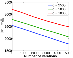
Figure 1: CSI when applied to a high-dimensional dataset with labels generated by sparse weight vector $\bm{w}_{\star}$ with sparsity level $k=\sqrt{d}$. Each of the three lines show how the $\ell_{2}$ error decreases with the number of iterations of the CSI algorithm. The covariates $\bm{x}_{1},\ldots,\bm{x}_{n}$ are sampled from $N(0,I_{d})$, where $n=500$. CSI is run with $\lambda=0.001,s=5k$. (best seen in color)

Conjecture 1.

Suppose we are given i.i.d. labeled data which satisfies the SIM $\mathbb{E}[y|X=x]=g_{\star}(\bm{w}_{\star}^{\top}\bm{x})$, where $g_{\star}$ is a $L-$ Lipschitz, monotonic function and $\|\bm{w}_{\star}\|_{0}\leq k$. Let $\Phi_{\star}^{\prime}\mbox{$\;\stackrel{{\scriptstyle\mbox{\rm def}}}{{=}}\;$}g_{\star}$ be $(\gamma_{l},\tau_{l})$ restricted strong convex and $(\gamma_{u},\tau_{u})$ restricted strong smooth, as defined in (?), for the given data distribution. Then with an appropriate choice of the parameters $\lambda$ and $s\geq k$, algorithm CSI with the hard-thresholding operation after $t$ iterations outputs a vector $\bm{w}_{t}$ that satisfies

$$||\bm{w}_{t}-\bm{w}_{\star}||_{2}\leq f(\gamma_{l},\gamma_{u})O\left(\frac{Lk\log(d)}{t}\right)+\Delta$$ (11)

where $\Delta$ is some function that depends on $k,\log(d),n,\tau_{l},\tau_{u}$ and $f(\gamma_{l},\gamma_{u})$ is some function dependent on $\gamma_{l},\gamma_{u}$ and is independent of $t$. $\Delta$ represents the statistical error of the iterates that arises due to the presence of limited data.

Conclusions and Discussion

In this paper, we introduced CSI , a unified algorithm to learn single index models in high dimensions, under general structural constraints on the data. The simplicity of our learning algorithm, its versatility, and competitive results makes it a great tool that can be added to a data analyst’s toolbox.

References

- [Abadi et al. 2016] Abadi, M.; Agarwal, A.; Barham, P.; Brevdo, E.; Chen, Z.; Citro, C.; Corrado, G. S.; Davis, A.; Dean, J.; Devin, M.; et al. 2016. Tensorflow: Large-scale machine learning on heterogeneous distributed systems. arXiv preprint arXiv:1603.04467.
- [Agarwal, Negahban, and Wainwright 2012] Agarwal, A.; Negahban, S. N.; and Wainwright, M. J. 2012. Fast global convergence of gradient methods for high-dimensional statistical recovery. The Annals of Statistics 40(5):2452–2482.
- [Alquier and Biau 2013] Alquier, P., and Biau, G. 2013. Sparse single-index model. The Journal of Machine Learning Research 14(1):243–280.
- [Argyriou, Evgeniou, and Pontil 2008] Argyriou, A.; Evgeniou, T.; and Pontil, M. 2008. Convex multi-task feature learning. Machine Learning 73(3):243–272.
- [Buja, Hastie, and Tibshirani 1989] Buja, A.; Hastie, T.; and Tibshirani, R. 1989. Linear smoothers and additive models. The Annals of Statistics 453–510.
- [Chandrasekaran et al. 2012] Chandrasekaran, V.; Recht, B.; Parrilo, P. A.; and Willsky, A. S. 2012. The convex geometry of linear inverse problems. Foundations of Computational Mathematics 12(6):805–849.
- [Cohen et al. 2012] Cohen, A.; Daubechies, I.; DeVore, R.; Kerkyacharian, G.; and Picard, D. 2012. Capturing ridge functions in high dimensions from point queries. Constructive Approximation 35(2):225–243.
- [Donoho 2006] Donoho, D. L. 2006. Compressed sensing. Information Theory, IEEE Transactions on 52(4):1289–1306.
- [Friedman and Stuetzle 1981] Friedman, J. H., and Stuetzle, W. 1981. Projection pursuit regression. Journal of the American statistical Association 76(376):817–823.
- [Ganti, Balzano, and Willett 2015] Ganti, R. S.; Balzano, L.; and Willett, R. 2015. Matrix completion under monotonic single index models. In Advances in Neural Information Processing Systems, 1864–1872.
- [Hastie et al. 2005] Hastie, T.; Tibshirani, R.; Friedman, J.; and Franklin, J. 2005. The elements of statistical learning: data mining, inference and prediction. The Mathematical Intelligencer 27(2):83–85.
- [Horowitz and Härdle 1996] Horowitz, J. L., and Härdle, W. 1996. Direct semiparametric estimation of single-index models with discrete covariates. Journal of the American Statistical Association 91(436):1632–1640.
- [Horowitz 2009] Horowitz, J. L. 2009. Semiparametric and nonparametric methods in econometrics. Springer.
- [Ichimura 1993] Ichimura, H. 1993. Semiparametric least squares (sls) and weighted sls estimation of single-index models. Journal of Econometrics 58(1):71–120.
- [Jacob, Obozinski, and Vert 2009] Jacob, L.; Obozinski, G.; and Vert, J.-P. 2009. Group lasso with overlap and graph lasso. In ICML, 433–440.
- [Jain, Tewari, and Kar 2014] Jain, P.; Tewari, A.; and Kar, P. 2014. On iterative hard thresholding methods for high-dimensional m-estimation. In Advances in Neural Information Processing Systems, 685–693.
- [Kakade et al. 2011] Kakade, S. M.; Kanade, V.; Shamir, O.; and Kalai, A. 2011. Efficient learning of generalized linear and single index models with isotonic regression. In Advances in Neural Information Processing Systems, 927–935.
- [Kalai and Sastry 2009] Kalai, A. T., and Sastry, R. 2009. The isotron algorithm: High-dimensional isotonic regression. In COLT.
- [Kingma and Ba 2014] Kingma, D., and Ba, J. 2014. Adam: A method for stochastic optimization. arXiv preprint arXiv:1412.6980.
- [Koren, Bell, and Volinsky 2009] Koren, Y.; Bell, R.; and Volinsky, C. 2009. Matrix factorization techniques for recommender systems. Computer (8):30–37.
- [Natarajan, Rao, and Dhillon 2015] Natarajan, N.; Rao, N.; and Dhillon, I. 2015. Pu matrix completion with graph information. In CAMSAP, 2015 IEEE 6th International Workshop on, 37–40. IEEE.
- [Negahban et al. 2012] Negahban, S. N.; Ravikumar, P.; Wainwright, M. J.; and Yu, B. 2012. A unified framework for high-dimensional analysis of m-estimators with decomposable regularizers. Statistical Science 27(4):538–557.
- [Park and Hastie 2007] Park, M. Y., and Hastie, T. 2007. L1-regularization path algorithm for generalized linear models. Journal of the Royal Statistical Society: Series B (Statistical Methodology) 69(4):659–677.
- [Plan, Vershynin, and Yudovina 2014] Plan, Y.; Vershynin, R.; and Yudovina, E. 2014. High-dimensional estimation with geometric constraints. arXiv preprint arXiv:1404.3749.
- [Radchenko 2015] Radchenko, P. 2015. High dimensional single index models. Journal of Multivariate Analysis 139:266–282.
- [Rao et al. 2016] Rao, N. S.; Nowak, R. D.; Cox, C. R.; and Rogers, T. T. 2016. Classification with the sparse group lasso. Signal Processing, IEEE Transactions on 64.
- [Rao, Shah, and Wright 2015] Rao, N.; Shah, P.; and Wright, S. 2015. Forward–backward greedy algorithms for atomic norm regularization. IEEE Transactions on Signal Processing 63(21):5798–5811.
- [Ravikumar et al. 2009] Ravikumar, P.; Lafferty, J.; Liu, H.; and Wasserman, L. 2009. Sparse additive models. JRSS: Series B 1009–1030.
- [Ryali et al. 2010] Ryali, S.; Supekar, K.; Abrams, D. A.; and Menon, V. 2010. Sparse logistic regression for whole-brain classification of fmri data. NeuroImage 51(2):752–764.
- [Tsybakov 2009] Tsybakov, A. 2009. Introduction to nonparametric estimation. Springer Verlag.
- [Van de Geer 2008] Van de Geer, S. A. 2008. High-dimensional generalized linear models and the lasso. The Annals of Statistics 614–645.
- [Zhou, Chen, and Ye 2011] Zhou, J.; Chen, J.; and Ye, J. 2011. MALSAR: Multi-tAsk Learning via StructurAl Regularization. Arizona State University.