On the Capacity and Performance of Generalized Spatial Modulation

Abstract

Generalized spatial modulation (GSM) uses $N$ antenna elements but fewer radio frequency (RF) chains ($R$) at the transmitter. Spatial modulation and spatial multiplexing are special cases of GSM with $R=1$ and $R=N$, respectively. In GSM, apart from conveying information bits through $R$ modulation symbols, information bits are also conveyed through the indices of the $R$ active transmit antennas. In this paper, we derive lower and upper bounds on the the capacity of a ($N,M,R$)-GSM MIMO system, where $M$ is the number of receive antennas. Further, we propose a computationally efficient GSM encoding (i.e., bits-to-signal mapping) method and a message passing based low-complexity detection algorithm suited for large-scale GSM-MIMO systems.

Keywords – GSM-MIMO capacity, GSM encoding, combinadics, low-complexity detection, message passing.

I Introduction

Spatial modulation (SM) is emerging as a promising multi-antenna modulation scheme (see [1] and the references therein). SM uses multiple antenna elements but only one radio frequency (RF) chain at the transmitter. The single-RF chain feature of SM brings in several advantages including reduced RF hardware complexity, size and cost, no spatial interference, and simple detection at the receiver, while offering the capacity and diversity benefits of multi-antenna systems. In SM, only one antenna element is activated in a given channel use and a QAM/PSK symbol is sent on the activated antenna; the remaining antenna elements remain silent. The index of the active antenna element also conveys information bits. It has been shown that SM can achieve better performance than spatial multiplexing (SMP) under certain conditions [1].

Generalized spatial modulation (GSM) is a generalization of SM, where the transmitter uses multiple ($N$) antenna elements and more than one ($R$) RF chain [2]. $R$ among the $N$ available antenna elements are activated in a given channel use, and $R$ QAM/PSK symbols are sent simultaneously on the active antennas. The indices of the $R$ active antennas also convey information bits. Both SM and SMP can be seen as special cases of GSM with $R=1$ and $R=N$, respectively. It has been shown that for a given modulation alphabet and $N$, there exists an optimum $R\leq N$ that maximizes the spectral efficiency [3]. Further, for the same spectral efficiency, GSM can perform better than both SM and SMP [4],[5]. This is illustrated in Fig. 1 which shows the bit error rate (BER) performance of maximum likelihood (ML) decoding for different configurations of MIMO systems each with $N=M=8$ and same spectral efficiency of 8 bits per channel use (bpcu). We can see that the (8,8,2)-GSM MIMO system outperforms both the (8,8,1)-system (i.e., SM system) and (8,8,8-system (i.e., SMP system). This superior performance of GSM-MIMO motivates us to study its capacity limits. While most studies on SM/GSM in the literature so far have focused mainly on performance analysis and receiver algorithms, capacity of SM/GSM systems remains to be studied. The need for capacity analysis of SM has also been highlighted in [1]. In [6], the authors have obtained the capacity of SM for MISO systems through simulation. However, an analytical characterization of the capacity of SM/GSM has not been explored. Our contribution in this paper addresses this gap. In particular, we derive lower and upper bounds on the capacity of GSM. Another contribution is the proposal of low complexity encoding (i.e., bits-to-GSM signal mapping) and detection methods suited for GSM-MIMO systems with large number of antennas and RF chains. The proposed encoding makes use of combinadic representations in combinatorial number system, and the detection makes use of layered message passing.

The rest of the paper is organized as follows. Section II introduces the GSM-MIMO system model. GSM-MIMO capacity bounds are derived in Section III. The proposed combinadics based GSM encoding scheme and the layered message passing based GSM detection scheme are presented in Section IV. Conclusions are presented in Section V.

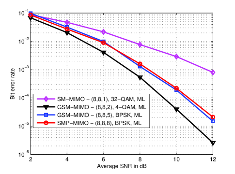
Figure 1: BER performance of different MIMO configurations with same spectral efficiency of 8 bpcu.

II GSM-MIMO system model

Consider a ($N,M,R$)-GSM MIMO system with $N$ antennas and $R$ RF chains at the transmitter ($1\leq R\leq N$), and $M$ antennas at the receiver. Figure 2 shows the GSM transmitter. An $R\times N$ switch connects the $R$ RF chains to the $N$ transmit antennas. In each channel use, $R$ out of $N$ transmit antennas are chosen and activated. The remaining $N-R$ antennas remain silent. The selection of the $R$ antennas to activate in a channel use is done based solely on $\lfloor\log_{2}{N\choose R}\rfloor$ information bits (not based on CSIT). Therefore, the indices of the active antennas convey $\lfloor\log_{2}{N\choose R}\rfloor$ information bits per channel use. On the active antennas, $R$ modulation symbols (one on each active antenna) from a modulation alphabet ${\mathbb{A}}$ are transmitted. This conveys $R\lfloor\log_{2}|{\mathbb{A}}|\rfloor$ additional information bits. Therefore, the total number of bits conveyed in a channel use in GSM is given by

$$\eta_{\scriptsize{\mbox{gsm}}}=\underbrace{R\left\lfloor\log_{2}{\mathbb{A}}\right\rfloor}_{\mbox{\scriptsize Modulation symbol bits}}+\underbrace{\bigg{\lfloor}\log_{2}{N\choose R}\bigg{\rfloor}}_{\mbox{\scriptsize Antenna index bits}}\quad\mbox{bpcu}.$$ (1)

II-A GSM signal set

Let ${\mathbb{G}}$ denote the GSM signal set, which is the set of all possible GSM signal vectors that can be transmitted. Therefore, if ${\bf x}$ is the $N\times 1$ signal vector transmitted by the GSM transmitter, then ${\bf x}\in{\mathbb{G}}$. For example, for $N=4$, $R=2$, and BPSK, i.e., ${\mathbb{A}}=\{\pm 1\}$, a GSM signal set can be as follows:

$${\mathbb{G}} = \left\{\begin{bmatrix}+1\\ +1\\ 0\\ 0\end{bmatrix},\begin{bmatrix}+1\\ -1\\ 0\\ 0\end{bmatrix},\begin{bmatrix}-1\\ -1\\ 0\\ 0\end{bmatrix},\begin{bmatrix}-1\\ +1\\ 0\\ 0\end{bmatrix},\begin{bmatrix}+1\\ 0\\ +1\\ 0\end{bmatrix},\begin{bmatrix}+1\\ 0\\ -1\\ 0\end{bmatrix},\begin{bmatrix}-1\\ 0\\ -1\\ 0\end{bmatrix},\begin{bmatrix}-1\\ 0\\ +1\\ 0\end{bmatrix},\right.$$

$$\left.\begin{bmatrix}+1\\ 0\\ 0\\ +1\end{bmatrix},\begin{bmatrix}+1\\ 0\\ 0\\ -1\end{bmatrix},\begin{bmatrix}-1\\ 0\\ 0\\ -1\end{bmatrix},\begin{bmatrix}-1\\ 0\\ 0\\ +1\end{bmatrix},\begin{bmatrix}0\\ +1\\ +1\\ 0\end{bmatrix},\begin{bmatrix}0\\ +1\\ -1\\ 0\end{bmatrix},\begin{bmatrix}0\\ -1\\ -1\\ 0\end{bmatrix},\begin{bmatrix}0\\ -1\\ +1\\ 0\end{bmatrix}\right\}.$$

Let ${\bf s}$ denote the $R\times 1$ vector of modulation symbols that are to be transmitted in a channel use over the $R$ chosen antennas, i.e., ${\bf s}\in{\mathbb{A}}^{R}$.

Definition: Define a matrix ${\bf A}$ of size $N\times R$ as the antenna activation pattern matrix. The matrix ${\bf A}$ represents a particular choice of $R$ antennas from the available $N$ antennas, such that the $N\times 1$ GSM signal vector ${\bf x}={\bf A}{\bf s}\in{\mathbb{G}}$. The matrix ${\bf A}$ is a sparse matrix consisting only of $1$’s and $0$’s, with exactly one non-zero entry in every column and one non-zero entry in $R$ rows. If $I_{1},I_{2},\cdots,I_{r},\cdots,I_{R}$ are the indices of the chosen antennas, then ${\bf A}$ is constructed as

$$A_{ij}=\left\{\begin{array}[]{ll}1&\mbox{if }j=r\mbox{ and }i=I_{r}\\ 0&\mbox{otherwise},\end{array}\right.$$ (2)

where $A_{ij}$ denotes the element in the $i$th row and $j$th column of ${\bf A}$.

Figure 2: GSM transmitter.

For example, in a system with $N=8$ and $R=4$, to activate antennas 1, 3, 6 and 8, the matrix ${\bf A}$ is given by

$${\bf A}\ =\ \left[\begin{array}[]{cccc}1&0&0&0\\ 0&0&0&0\\ 0&1&0&0\\ 0&0&0&0\\ 0&0&0&0\\ 0&0&1&0\\ 0&0&0&0\\ 0&0&0&1\\ \end{array}\right].$$ (3)

Note that the indices of the non-zero rows in matrix ${\bf A}$ give the support of the GSM signal vector ${\bf x}$. Out of the $N\choose R$ possible antenna activation choices, only $2^{\lfloor\log_{2}{N\choose R}\rfloor}$ are needed for signaling. Let ${\cal A}$ denote this set of all allowed antenna activation pattern matrices, where $|{\cal A}|=2^{\lfloor\log_{2}{N\choose R}\rfloor}$ and ${\bf A}\in{\cal A}$. Let $L\triangleq|{\cal A}|$. Now, ${\mathbb{G}}$ is given by

$${\mathbb{G}}=\big{\{}{\bf x}:{\bf x}={\bf A}{\bf s},\mbox{ for some }{\bf A}\in{\cal A},{\bf s}\in{\mathbb{A}}^{R}\big{\}}.$$ (4)

Note that any GSM signal vector ${\bf x}_{j}\in{\mathbb{G}}$, $j=1,\cdots,|{\mathbb{G}}|$, can be represented as ${\bf x}_{j}={\bf A}_{i}{\bf s}_{k}$ with some ${\bf A}_{i}\in{\cal A}$, $i=1,\cdots,|{\cal A}|$ and ${\bf s}_{k}\in{\mathbb{A}}^{R}$, $k=1,\cdots,|{\mathbb{A}}|^{R}$, and $|{\mathbb{G}}|=|{\cal A}||{\mathbb{A}}|^{R}$. Conversely, given any ${\bf A}_{i}\in{\cal A}$ and ${\bf s}_{k}\in{\mathbb{A}}^{R}$, there exists a GSM signal vector ${\bf x}_{j}\in{\mathbb{G}}$ such that ${\bf x}_{j}={\bf A}_{i}{\bf s}_{k}$. Since ${\bf A}_{i}$ and ${\bf s}_{k}$ are chosen by two independent information bit sequences, ${\bf A}_{i}$ and ${\bf s}_{k}$ are independent. That is, $p({\bf x})=p({\bf A}{\bf s})=p({\bf A})p({\bf s})$. Thus, the above system model of GSM-MIMO decouples the choice of active antennas and the transmitted modulation symbols into two independent random variables, namely ${\bf A}$ and ${\bf s}$. This makes the GSM-MIMO system analysis simpler.

The $M\times 1$ received signal vector ${\bf y}=[y_{1}\ y_{2}\cdots\ y_{M}]^{T}$ at the receiver can be written as

$${\bf y} = {\bf H}{\bf x}+{\bf w}\ =\ {\bf H}{\bf A}{\bf s}+{\bf w},$$ (5)

where ${\bf x}\in{\mathbb{G}}$ is the transmit vector, ${\bf H}\in\mathbb{C}^{M\times N}$ is the channel gain matrix whose $(i,j)$th entry $H_{i,j}\sim\mathcal{CN}(0,1)$ denotes the complex channel gain from the $j$th transmit antenna to the $i$th receive antenna, and ${\bf w}=[w_{1}\ w_{2}\cdots\ w_{M}]^{T}$ is the noise vector whose entries are modeled as complex Gaussian with zero mean and variance $\sigma^{2}$. Since ${\bf x}$ is obtained based only on $\eta_{\scriptsize{\mbox{gsm}}}$ information bits, ${\bf x}$ and ${\bf H}$ are independent. Since ${\bf x}={\bf A}{\bf s}$, ${\bf A}{\bf s}$ and ${\bf H}$ are independent. Also, ${\bf A}$ and ${\bf s}$ are independent. So, ${\bf A}$ and ${\bf H}$ are independent. So, the mutual information between ${\bf x}$ and ${\bf y}$ in GSM is given by $I({\bf x};{\bf y}|{\bf H})=I({\bf A},{\bf s};{\bf y}|{\bf H})$.

III GSM-MIMO capacity bounds

The capacity of a spatially multiplexed $M\times N$ MIMO channel with channel state information at the receiver is [7]

$$C={\mathbb{E}}_{{\bf H}}\Big{\{}\log_{2}\big{[}\det({\bf I}_{M}+\frac{1}{\sigma^{2}}{\bf H}{\bf\Phi}{\bf H}^{H})\big{]}\Big{\}},$$ (6)

where ${\bf\Phi}$ is the covariance matrix of the transmit signal vector with elements from Gaussian codebook. For i.i.d. modulation symbols and total power $\sigma^{2}_{x}$, the capacity expression becomes

$$C={\mathbb{E}}_{{\bf H}}\Big{\{}\log_{2}\big{[}\det({\bf I}_{M}+\frac{\sigma^{2}_{x}}{N\sigma^{2}}{\bf H}{\bf H}^{H})\big{]}\Big{\}}.$$ (7)

Here, we are interested in the capacity of GSM-MIMO, where the symbols sent on the active antennas are from Gaussian codebook. The capacity of GSM-MIMO can be written as

$$C_{GSM} = {\mathbb{E}}_{{\bf H}}(I({\bf x};{\bf y}))$$ (8)

$$= {\mathbb{E}}_{{\bf H}}(h({\bf y})-h({\bf y}|{\bf x}))={\mathbb{E}}_{{\bf H}}(h({\bf y})-h({\bf w}))$$

$$= {\mathbb{E}}_{{\bf H}}(h({\bf y})-\log_{2}[\det(\pi e\sigma^{2}{\bf I}_{M})]),$$

where $h(.)$ denotes the differential entropy. To compute $C_{GSM}$, we need to evaluate $h({\bf y})$, which requires the knowledge of the distribution of ${\bf y}$. From (5), we can see that the distribution of ${\bf y}$ is a Gaussian mixture given by

$$p({\bf y}) = \sum_{i=1}^{L}p({\bf y},{\bf A}_{i})=\sum_{i=1}^{L}p({\bf y}|{\bf A}_{i})p({\bf A}_{i})$$ (9)

$$= \sum_{i=1}^{L}{\mathcal{N}}({\boldsymbol{\mu}}_{i},{\bf\Phi}_{i})p_{i},$$

where

$$p_{i} = p({\bf A}_{i}),\quad\quad{\bf A}_{i}\in{\cal A},\quad\quad i=1,2,\cdots,L,$$ (10)

$${\boldsymbol{\mu}}_{i} = {\mathbb{E}}({\bf y}|{\bf A}_{i})$$ (11)

$$= {\mathbb{E}}({\bf H}{\bf A}_{i}{\bf s}+{\bf w}|{\bf A}_{i})={\bf 0},$$

$${\bf\Phi}_{i} = {\mathbb{E}}({\bf y}{\bf y}^{H}|{\bf A}_{i})={\mathbb{E}}[({\bf H}{\bf A}_{i}{\bf s}+{\bf w})({\bf H}{\bf A}_{i}{\bf s}+{\bf w})^{H}|{\bf A}_{i}]$$ (12)

$$= {\bf H}{\bf A}_{i}{\mathbb{E}}_{{\bf s}}({\bf s}{\bf s}^{H}){\bf A}_{i}^{H}{\bf H}^{H}+\sigma^{2}{\bf I}_{M}.$$

If all the possible antenna activation patterns are equally likely, then $p_{i}=\frac{1}{L}$. When the transmitted modulation symbols are independent of each other, ${\mathbb{E}}({\bf s}{\bf s}^{H})=\frac{\sigma^{2}_{x}}{R}{\bf I}_{R}$, Now, (9) becomes

$${\bf y}\sim\frac{1}{L}\sum_{i=1}^{L}{\mathcal{N}}\Big{(}{\bf 0},\frac{\sigma^{2}_{x}}{R}{\bf H}{\bf A}_{i}{\bf A}_{i}^{H}{\bf H}^{H}+\sigma^{2}{\bf I}_{M}\Big{)}.$$ (13)

The differential entropy of ${\bf y}$ is given by

$$h({\bf y})=-\frac{1}{L}\sum_{i=1}^{L}\int_{{\bf y}}{\mathcal{N}}({\bf 0},{\bf\Phi}_{i})\log_{2}\Big{(}\frac{1}{L}\sum_{i=1}^{L}{\mathcal{N}}({\bf 0},{\bf\Phi}_{i})\Big{)}d{\bf y}.$$ (14)

It is difficult to get a closed-form solution to the above expression. Hence, we try to bound it above and below by the following techniques.

Lower bound 1, $L_{1}$: Since $-\log(.)$ is a convex function, by Jensen’s inequality,

$${\mathbb{E}}[-\log p(y)]\geq-\log{\mathbb{E}}[p(y)].$$

Hence, the differential entropy $h({\bf y})$ can be lower bounded as

$$h({\bf y}) = {\mathbb{E}}[-\log_{2}p({\bf y})]$$

$$\geq -\log_{2}\int p^{2}({\bf y})d{\bf y}$$

$$= -\log_{2}\int\Big{(}\frac{1}{L}\sum_{i=1}^{L}{\mathcal{N}}({\bf 0},{\bf\Phi}_{i})\Big{)}^{2}d{\bf y}$$

$$= -\log_{2}\bigg{\{}\frac{1}{L^{2}\pi^{M}}\sum_{i=1}^{L}\sum_{j=1}^{L}\frac{\det(({\bf\Phi}_{i}^{-1}+{\bf\Phi}_{j}^{-1})^{-1})}{\det({\bf\Phi}_{i})\det({\bf\Phi}_{j})}$$

$$\hskip 56.9055pt\underbrace{\int\frac{e^{-{\bf y}^{H}({\bf\Phi}_{i}^{-1}+{\bf\Phi}_{j}^{-1}){\bf y}}}{\pi^{M}\det(({\bf\Phi}_{i}^{-1}+{\bf\Phi}_{j}^{-1})^{-1})}d{\bf y}}_{=1}\bigg{\}}$$

$$= -\log_{2}\bigg{\{}\frac{1}{L^{2}\pi^{M}}\sum_{i=1}^{L}\sum_{j=1}^{L}\frac{1}{\det({\bf\Phi}_{i}+{\bf\Phi}_{j})}\bigg{\}}$$

$$\triangleq l_{1}.$$

From (8) and (III), a lower bound on $C_{GSM}$ can be obtained as

$$C_{GSM}\geq L_{1}\triangleq{\mathbb{E}}_{{\bf H}}(l_{1}-\log_{2}\det(\pi e\sigma^{2}{\bf I}_{M})).$$ (16)

Lower bound 2, $L_{2}$: Since differential entropy is a concave function, we can write

$$h({\bf y}) = h\Big{(}\frac{1}{L}\sum_{i=1}^{L}{\mathcal{N}}({\bf 0},{\bf\Phi}_{i})\Big{)}$$

$$\geq \frac{1}{L}\sum_{i=1}^{L}h\big{(}{\mathcal{N}}({\bf 0},{\bf\Phi}_{i})\big{)}=\frac{1}{L}\sum_{i=1}^{L}\log_{2}\det\big{(}\pi e{\bf\Phi}_{i})\triangleq l_{2}.$$

From the above equation, $C_{GSM}$ can be lower bounded as

$$C_{GSM}\geq L_{2}\triangleq{\mathbb{E}}_{{\bf H}}(l_{2}-\log_{2}\det(\pi e\sigma^{2}{\bf I}_{M})).$$ (17)

Based on the two lower bounds $L_{1}$ and $L_{2}$, a refined lower bound on GSM-MIMO capacity is given by

$$C_{GSM}\geq L\triangleq\text{max}(L_{1},L_{2}).$$ (18)

Upper bound 1, $U_{1}$: By the property of entropy, we can write

$$h({\bf y},{\bf A}) = -\sum_{\forall{\bf A}}\int p({\bf y},{\bf A})\log_{2}p({\bf y},{\bf A})d{\bf y}$$

$$= -\sum_{\forall{\bf A}}\int p({\bf y},{\bf A})\log_{2}p({\bf y}|{\bf A})d{\bf y}$$

$$-\sum_{\forall{\bf A}}\log_{2}p({\bf A})\int p({\bf y},{\bf A})d{\bf y}$$

$$= h({\bf y}|{\bf A})+H({\bf A}).$$

Further, we also have

$$h({\bf y}) = h({\bf y},{\bf A})-h({\bf A}|{\bf y})\leq h({\bf y},{\bf A}).$$

Using the above properties, an upper bound for $h({\bf y})$ can be written as

$$h({\bf y}) \leq h({\bf y},{\bf A})=h({\bf y}|{\bf A})+H({\bf A})$$

$$= \int\sum_{\forall{\bf A}}p({\bf y},{\bf A})\log_{2}\frac{p({\bf A})}{p({\bf y},{\bf A})}d{\bf y}+\sum_{i=1}^{L}-p_{i}\log_{2}p_{i}$$

$$= \frac{1}{L}\sum_{i=1}^{L}\log_{2}\det\big{(}\pi e{\bf\Phi}_{i})+\log_{2}L\triangleq u_{1}.$$

Now, an upper bound on $C_{GSM}$ can be written as

$$C_{GSM}\leq U_{1}\triangleq{\mathbb{E}}_{{\bf H}}(u_{1}-\log_{2}\det(\pi e\sigma^{2}{\bf I}_{M})).$$ (19)

Upper bound 2, $U_{2}$: Here, we approximate the probability distribution of ${\bf y}$ to a Gaussian distribution. This leads to an upper bound because the entropy of any random variable is bounded above by the entropy of a Gaussian random variable with the same mean and variance. The mean and covariance of ${\bf y}$ are given by

$${\mathbb{E}}({\bf y}) = {\bf 0},$$

$${\mathbb{E}}({\bf y}{\bf y}^{H}) = {\bf H}{\mathbb{E}}_{{\bf A}}[{\bf A}_{i}{\mathbb{E}}_{{\bf s}}({\bf s}{\bf s}^{H}){\bf A}_{i}^{H}]{\bf H}^{H}+\sigma^{2}{\bf I}_{M}$$ (20)

$$= {\bf H}\bigg{(}\frac{1}{L}\sum_{i=1}^{L}{\bf A}_{i}\Big{(}\frac{\sigma^{2}_{x}}{R}{\bf I}_{R}\Big{)}{\bf A}_{i}^{H}\bigg{)}{\bf H}^{H}+\sigma^{2}{\bf I}_{M}$$

$$= \frac{\sigma^{2}_{x}}{RL}{\bf H}\Big{(}\sum_{i=1}^{L}{\bf D}_{i}\Big{)}{\bf H}^{H}+\sigma^{2}{\bf I}_{M},$$

where ${\bf D}_{i}\triangleq{\bf A}_{i}{\bf A}^{H}_{i}$. Let $\{I_{1}^{i},I_{2}^{i},\cdots,I_{r}^{i},\cdots,I_{R}^{i}\}$ be the set of active antenna indices that corresponds to the antenna activation pattern matrix ${\bf A}_{i}$. It can then be seen that ${\bf D}_{i}$ is a diagonal matrix, such that

$$(D_{i})_{j,k}=\left\{\begin{array}[]{ll}1&\mbox{if }j=k=I\in\{I_{1}^{i},I_{2}^{i},\cdots,I_{R}^{i}\}\\ 0&\mbox{otherwise},\end{array}\right.$$

where $(D_{i})_{j,k}$ is the element in the $j$th row and $k$th column of ${\bf D}_{i}$. Assuming that all $N\choose R$ activation patterns are allowed, i.e., $|{\cal A}|=L={N\choose R}$, the number of times any particular antenna will be active among the $N\choose R$ activation patterns is $N-1\choose R-1$. Therefore, ${\bf D}={N-1\choose R-1}{\bf I}_{N}$ and (20) becomes

$${\mathbb{E}}({\bf y}{\bf y}^{H}) = \frac{\sigma^{2}_{x}}{N}{\bf H}{\bf H}^{H}+\sigma^{2}{\bf I}_{M}\triangleq\Phi^{\prime}.$$

Now, an upper bound on the GSM-MIMO capacity is given by

$$C_{GSM} \leq U_{2}\triangleq{\mathbb{E}}_{{\bf H}}(\log_{2}\det(\pi e\Phi^{\prime})-\log_{2}\det(\pi e\sigma^{2}{\bf I}_{M}))$$ (21)

$$= {\mathbb{E}}_{{\bf H}}\Big{\{}\log_{2}\big{[}\det({\bf I}_{M}+\frac{\sigma^{2}_{x}}{N\sigma^{2}}{\bf H}{\bf H}^{H})\big{]}\Big{\}},$$

which is the same as the capacity of a $M\times N$ spatially multiplexed MIMO system.

Based on the two upper bounds $U_{1}$ and $U_{2}$, a refined upper bound on GSM capacity can be obtained as

$$C_{GSM}\leq U\triangleq\text{min}(U_{1},U_{2}).$$ (22)

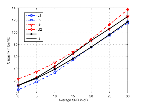
Figure 3: Capacity bounds for GSM-MIMO system with $N=16,R=12$, and $M=16.$

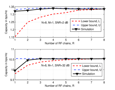
Figure 4: Comparison of simulated capacity and bounds for GSM-MIMO system with $N=8$, $M=1$, and varying $R$.

Numerical results: We evaluated the lower and upper bounds on the GSM-MIMO capacity for different system configurations. Figure 3 shows the lower and upper bounds for GSM-MIMO systems with $N=16$, $R=12$, $M=16$. We see that the lower bound $L_{2}$ and upper bound $U_{2}$ are tighter at low SNRs. Whereas, the lower bound $L_{1}$ and upper bound $U_{1}$ are tighter at high SNRs. It can be noted from the figure that the lower and upper bounds are very close at low SNRs; so, in this regime, the GSM-MIMO capacity is almost same as that of a spatially multiplexed MIMO system with the same $N$ and $M$. In Fig. 4, we compare the bounds on GSM-MIMO capacity with the true GSM-MIMO capacity obtained through simulation. We consider GSM-MIMO with $N=8$, $M=1$, SNR $=2,32$ dB, and varying $R$. In the top figure of Fig. 4, we observe that, at SNR = 2 dB, the gap between the upper and lower bounds is $U-L=0.188$ bps/Hz for $R=1$ and $U-L<10^{-2}$ bps/Hz for $R>5$. Also, in the bottom figure of Fig. 4, at SNR = 32 dB, the gap is $U-L=0.782$ bps/Hz for $R=1$ and $U-L<10^{-2}$ bps/Hz for $R>6$.

IV Low-complexity GSM-MIMO encoding/decoding

It is known that large-scale MIMO systems provide a variety of advantages [8]. However, for large values of $N,M,R$ in GSM-MIMO, the encoding and decoding complexities become prohibitively large. In this section, we propose low-complexity methods to encode and detect GSM signals that scale well for large $N,M,R$.

IV-A GSM encoding using combinadics

In GSM-MIMO, $\lfloor\log_{2}{N\choose R}\rfloor$ bits are used to choose an activation pattern matrix ${\bf A}$ from ${\cal A}$, and $R\left\lfloor\log_{2}{\mathbb{A}}\right\rfloor$ bits are used to generate ${\bf s}$ from ${\mathbb{A}}^{R}$. While the mapping of $R\left\lfloor\log_{2}{\mathbb{A}}\right\rfloor$ bits to modulation symbols in ${\bf s}$ is straight-forward, the mapping of $\lfloor\log_{2}{N\choose R}\rfloor$ bits to a choice of activation pattern is not. A table or a map of bit sequence to activation patterns has to be maintained both at the transmitter and receiver. For large values of $N,M,R$, the size of this map can become prohibitively large. For example, if $N=64,R=32$, then $|{\cal A}|={64\choose 32}\approx 1.83\times 10^{18}\approx 2^{60}$. Implementation of an encoding map of this size is impractical. To alleviate this problem, we use combinadic representations in combinatorial number system.

Definition: The combinadic of a number $n\in[0,{N\choose R}-1]$ is the $R$-tuple $(N_{1},N_{2},\cdots,M)$ such that $n=\sum_{i=1}^{R}{N_{i}\choose i}$ and $N_{1}<N_{2}<\cdots<M<N$.

The values of $N_{i}$ for a given $n$ can be obtained as [9]

$$N_{i}=\mbox{Largest non-negative integer s.t. }n-\sum_{j=i}^{R}{N_{j}\choose j}\geq 0.$$

The following encoding procedure maps the bits to antenna activation pattern in GSM. Let $\eta_{a}\triangleq\lfloor\log_{2}{N\choose R}\rfloor$.

1. Accumulate $\eta_{a}$ bits to form the bit sequence ${\bf b}=[b_{\eta_{a}-1},\cdots,b_{1},b_{0}]$. Obtain $g({\bf b})=\sum_{i=0}^{\eta_{a}-1}2^{i}b_{i}$.

2. Find the combinadic of $g({\bf b})$.

3. Construct ${\bf A}$ matrix such that the indices of the $R$ non-zero rows of ${\bf A}$ are given by the combinadic of $g({\bf b})$.

An example of the encoding map for $N=4,R=3$ based of the above procedure is illustrated in Table I. The demapping procedure is listed below.

1. Obtain the combinadic corresponding to the decoded antenna activation pattern matrix.

2. Compute $g(\hat{{\bf b}})$ from this combinadic as $g(\hat{{\bf b}})=\sum\limits_{i=1}^{R}{N_{i}\choose i}$.

3. Demap $g(\hat{{\bf b}})$ to get $\hat{{\bf b}}$.

The above low complexity mapping/demapping procedures allow practical implementation of GSM encoding for large $N,M,R$.

${\bf b}$	$g({\bf b})$	combinadic of $g({\bf b})$	Active antenna
		$(N_{1},N_{2},N_{3})$	indices
$00$	$0$	$(0,1,2)$	$(1,2,3)$
$01$	$1$	$(0,1,3)$	$(1,2,4)$
$10$	$2$	$(0,2,3)$	$(1,3,4)$
$11$	$3$	$(1,2,3)$	$(2,3,4)$

TABLE I: Encoding map for GSM system with $N=4,R=3$.

Example: Let $n_{t}=10,n_{rf}=4$. Then, $|{\cal A}|=2^{7}=128$.
Mapping: Let ${\bf b}=[0010011]$ be the bit sequence that is to be transmitted. The decimal equivalent of ${\bf b}$ is $d({\bf b})=19$, and the combinadic of $19$ is $(N_{1},N_{2},N_{3},N_{4})=(0,1,4,6)$. The corresponding indices of the activated antennas are $(1,2,5,7)$.
Demapping: Let $(3,4,5,6)$ be the detected antenna activity pattern at the receiver. The combinadic of this antenna activity pattern is $(2,3,4,5)$, and the decimal equivalent is $14$. The bit sequence for this decimal value of 14 is $[0001110]$. This gives the corresponding bit sequence of the detected antenna activity pattern at the receiver.

IV-B GSM Detection: Layered message passing algorithm

The maximum a posteriori probability (MAP) detection rule for GSM-MIMO is given by

$$\hat{{\bf x}}=\mathop{\text{argmax}}_{{\bf x}\in{\mathbb{G}}}\ p({\bf x}\mid{\bf y}).$$ (23)

Note that, $|{\mathbb{G}}|=2^{\eta_{\scriptsize{\mbox{gsm}}}}$. Therefore, the exact computation of (23) requires exponential complexity in $N,R$. To address this problem, here we propose a low complexity layered message passing (LaMP) algorithm which gives an approximate solution to (23). In the proposed LaMP algorithm, we define four sets of nodes and exchange messages between them in layers. There are two layers of message exchanges, one corresponds to the detection of modulation symbols and the other corresponds to the detection of the antenna activation pattern. In order to describe this algorithm, we define a new variable as follows.

Definition: A variable $a_{i}$ is called the antenna activity indicator if $a_{i}=1$ if the $i$th antenna is active, else $a_{i}=0$. That is, $a_{i}={\bf 1}_{\{i\text{th antenna is active}\}}$, where ${\bf 1}$ is the indicator function.

Therefore, $x_{i}=a_{i}s,s\in{\mathbb{A}}$. Note that $\sum_{i=1}^{N}a_{i}=R$, which we call as the GSM system constraint $G$. Let ${\bf a}\triangleq[a_{1},a_{2},\cdots,a_{N}]$. Now, $p({\bf x}\mid{\bf y})$ in (23) can be written as

$$p({\bf x},{\bf a}|{\bf y}) \propto p({\bf y}|{\bf x},{\bf a})p({\bf x},{\bf a})$$ (24)

$$= p({\bf y}|{\bf x})p({\bf x}|{\bf a})p({\bf a})$$

$$= \Big{\{}\prod_{j=1}^{M}p(y_{i}|{\bf x})\prod_{i=1}^{N}p(x_{i}|a_{i})\Big{\}}p({\bf a}).$$

Thus, by defining a new layer of variables $a_{i}$s corresponding to antenna activity, we have effectively decoupled the dependences present among the elements of the transmit vector ${\bf x}$. Based on (24), we model the GSM-MIMO system as a graph with four types of nodes, namely,

• $M$ observation nodes corresponding to the elements of ${\bf y}$,

• $N$ variable nodes corresponding to the elements of ${\bf x}$,

• $N$ antenna activity nodes corresponding to the elements of ${\bf a}$, and

• a constraint node corresponding to the GSM constraint $G$.

This is illustrated in Fig. 5. On this graph, we iteratively pass messages between the nodes and obtain the marginal probabilities of the transmitted symbols.

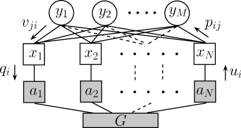
Figure 5: Graphical model and messages passed in the proposed LaMP detector.

The different messages passed in this graph are

1. $v_{ji}$: from observation node $y_{j}$ to variable node $x_{i}$,

2. $p_{ij}$: from variable node $x_{i}$ to observation node $y_{j}$,

3. $q_{i}$: from variable node $x_{i}$ to antenna activity node $a_{i}$, and

4. $u_{i}$: from antenna activity node $a_{i}$ to variable node $x_{i}$.

The messages are exchanged between two layers, namely,

1. Layer 1: observation nodes and variable nodes (denoted by unshaded nodes in Fig 5); this layer generates approximate a posteriori probabilities of the individual elements of ${\bf x}$, and

2. Layer 2: antenna activity nodes and GSM constraint node (denoted by shaded nodes in Fig 5); this layer generates approximate a posteriori probabilities of the individual elements of ${\bf a}$.

In constructing the messages at the variable nodes, we employ a Gaussian approximation of the interference as described below. This significantly reduces the detection complexity. From (5), we can write

$$y_{j}=H_{ji}x_{i}+g_{ji},\quad g_{ji}\triangleq\sum_{l=1\atop{l\neq i}}^{N}H_{jl}x_{l}+w_{j}.$$ (25)

where $i=1,2,\cdots,N$ and $j=1,2,\cdots,M$. We approximate $g_{ji}$ to be Gaussian. Then,

$$\mu_{ji} \triangleq {\mathbb{E}}(g_{ji})$$ (26)

$$= \sum_{l\neq i}H_{jl}{\mathbb{E}}(x_{l})$$

$$= \sum_{l\neq i}H_{jl}\sum_{x\in{\mathbb{A}}\cup 0}xp_{ij}(x),$$

and

$$\sigma_{ji}^{2} \triangleq \mbox{Var}(g_{ji})$$ (27)

$$= \sigma^{2}+\sum_{l\neq i}H_{jl}^{2}\mbox{Var}(x_{l})$$

$$= \sum_{l\neq i}H_{jl}^{2}\sum_{x\in{\mathbb{A}}\cup 0}x^{2}p_{ij}(x).$$

Using the above approximation, we derive the messages as follows.

Layer 1:

$$v_{ji}(x) \triangleq \Pr(x_{i}=x|y_{j})$$ (28)

$$\approx \frac{1}{\sigma_{ji}^{2}\sqrt{2\pi}}\exp\Big{(}\frac{-(y_{j}-\mu_{ji}-H_{ji}x)^{2}}{2\sigma_{ji}^{2}}\Big{)},$$

The APP of the individual elements of ${\bf x}$ is given by

$$p_{ij}(x) \triangleq \Pr(x_{i}=x|{\bf y}_{\setminus j})$$ (29)

$$\approx \prod_{k=1\atop{k\neq j}}^{M}\Pr(x_{i}=x|y_{k})$$

$$\propto u_{i}(x^{\odot})\prod_{k\neq j}v_{ki}(x),$$

where ${\bf y}_{\setminus j}$ denotes the set of all elements of ${\bf y}$ except $y_{j}$, and

$$x^{\odot}=\left\{\begin{array}[]{ll}0&\mbox{if }x=0\\ 1&\mbox{else}.\end{array}\right.$$

The inclusion of $u_{i}(.)$ in the computation of this APP helps us to relieve the elements of ${\bf x}$ from the dependencies on the antenna activity pattern.

Layer 2: The APP estimate of $a_{i}$ from the variable nodes is

$$q_{i}(b) \triangleq \Pr(a_{i}=b|{\bf x})$$ (32)

$$\approx \left\{\begin{array}[]{ll}\sum\limits_{x\in{\mathbb{A}}}\prod\limits_{k=1}^{M}\Pr(x_{i}=x|y_{k}),&\mbox{if }b=1\\ \prod\limits_{k=1}^{M}\Pr(x_{i}=0|y_{k}),&\mbox{if }b=0\end{array}\right.$$

$$\propto \left\{\begin{array}[]{ll}\sum\limits_{x\in{\mathbb{A}}}\prod\limits_{k=1}^{M}v_{ki}(x)&\mbox{if }b=1\\ \prod\limits_{k=1}^{M}v_{ki}(0),&\mbox{if }b=0,\end{array}\right.$$ (35)

The APP estimate of $a_{i}$ after processing GSM constraint $G$ is

$$u_{i}(b) \triangleq \Pr(a_{i}=b|{\bf x}_{\setminus i})$$ (38)

$$\propto \left\{\begin{array}[]{ll}\Pr(\sum\limits_{l\neq i}a_{l}=R-1|{\bf a}_{\setminus i}),&\mbox{if }b=1\\ \Pr(\sum\limits_{l\neq i}a_{l}=R|{\bf a}_{\setminus i}),&\mbox{if }b=0\end{array}\right.$$

$$\approx \left\{\begin{array}[]{ll}\phi_{i}(R-1)&\mbox{if }b=1\\ \phi_{i}(R)&\mbox{if }b=0,\end{array}\right.$$ (41)

where $\Pr(\sum\limits_{l=1,l\neq i}^{N}a_{l}=R-1|{\bf a}_{\setminus i})$ denotes the probability that the antenna activity pattern satisfies the GSM signal constraint $G$ (i.e., $\sum_{i=1}^{N}a_{i}=R$) given that the $i$th antenna is active, and $\Pr(\sum\limits_{l=1,l\neq i}^{N}a_{l}=R|{\bf a}_{\setminus i})$ denotes the probability that the antenna activity pattern satisfies $G$ given that the $i$th antenna is not active. Since this probability involves the summation of $N-1$ random variables, it is evaluated as $\phi_{i}=\bigotimes\limits_{l=1\atop{l\neq i}}^{N}q_{l}$, where $\bigotimes$ is the convolution operation, and $\phi_{i}(.)$ is a probability mass function with probability masses at $N$ points ($0,1,2,\cdots,N-1$).

Message passing: The schedule of the messages passed in the LaMP algorithm is as follows:

1. Intiliaze $p_{ij}(x)=\frac{1}{|{\mathbb{A}}\cup 0|}$ and $q_{i}(b)=\frac{R}{N}$, $\forall x,b,i,j$.

2. Compute $v_{ji}(x)$, $\forall x,i,j$.

3. Compute $u_{i}(b)$, $\forall b,i$.

4. Compute $p_{ij}(x)$, $\forall x,i,j$.

5. Compute $q_{i}(b)$, $\forall b,i$.

6. Perform damping of messages $p_{ji}(x)$ and $q_{i}(b)$ with a damping factor $\Delta$.

This completes one iteration of the LaMP algorithm. These steps are repeated until a fixed number of iterations are reached.

Complexity of LaMP: The computational complexities of evaluating the messages $v_{ji}(x)$, $p_{ij}(x)$, and $q_{i}(b)$ are of order $O(MN|{\mathbb{A}}|)$ per iteration of the LaMP algorithm. Because of the $N-1$ convolutions required for each of the $N$ antenna activity indicators, a naive method of computing $u_{i}(b)$ will result in a computational complexity of order $O(N^{3}+N^{2})$. To reduce this complexity, we propose the following techniques.

1. Deconvolution: In this technique, at every iteration, we first compute $\phi_{0}=\bigotimes\limits_{i=1}^{N}q_{i}$, which gives a probability mass function with $N+1$ points $(0,1,\cdots,N)$. To evaluate each $\phi_{i}$, we deconvolve $q_{i}$ from $\phi_{0}$, which gives the required probability mass function with $N$ points. This method has a computational complexity of order $O(N^{2}+N)$. A disadvantage of this method is that, in a limited precision system, the deconvolution operation is not numerically stable. Because of this reason, deconvolution may some times result in negative values to probabilities. To avoid this limitation in fixed precision systems, we can employ one of the following techniques.

2. Using FFT: Since Fourier transform converts convolution to multiplication in the transformed domain, FFT can be exploited for reducing the complexity in computing $u_{i}(b)$. First, we obtain $Q_{i}$, an $N$-point FFT of $q_{i},\forall i$. Then, we compute $\phi_{f}=\Pi_{i=1}^{N}Q_{i}$. Now, to evaluate each $\phi_{i}$ we compute IFFT$(\frac{\phi_{f}}{Q_{i}})$, which gives the required probability mass function with $N$ points. This method has a computational complexity of order $O(N^{2}+N)$. It is noted that the Fourier transform preserves only the total power in a signal (a consequence of Parseval’s theorem) and not the sum of amplitudes, i.e., $\sum_{\forall k}Q_{i}(k)\neq\sum_{\forall k}q_{i}(k)=1$. Thus, in order to satisfy the condition of total probability being $1$, every $\phi_{i}$ computation requires a normalization. This marginally increases the computations required compared to the previous technique.

3. Gaussian approximation: To compute $u_{i}(b)$, we require $N-1$ probability mass functions, i.e., $q_{i}$s. We note that $q_{i}$ is a Bernoulli distribution with probability masses for $a_{i}=0$ and $a_{i}=1$, i.e., $\Pr(a_{i}=0|{\bf x})=q_{i}(0)$ and $\Pr(a_{i}=1|{\bf x})=q_{i}(1)$. The evaluation of $\phi_{i}$ requires the computation of the distribution of the random variable $\sum\limits_{l=1,l\neq i}^{N}a_{l}$, where the antenna activity indicator $a_{i}$ is distributed according to the Bernoulli distribution $q_{i}$. For large $N$, the distribution of this sum is approximately Gaussian with mean $m_{i}$ and variance $c_{i}$, where

$$m_{i}={\mathbb{E}}\bigg{(}\sum_{l=1,l\neq i}^{N}a_{i}\bigg{)}=\sum_{l=1,l\neq i}^{N}q_{l}(1),$$

$$c_{i}=\text{Var}\bigg{(}\sum_{l=1,l\neq i}^{N}a_{i}\bigg{)}=\sum_{l=1,l\neq i}^{N}q_{l}(0)q_{l}(1).$$

Let $g_{i}\triangleq{\mathcal{N}}(m_{i},c_{i})$. Then, $u_{i}(1)\propto g_{i}(R-1)$ and $u_{i}(0)\propto g_{i}(R)$. The computational complexity of this technique is of order $O(N)$. From simulations, we observed that the LaMP algorithm requires a few more number of iterations to converge when this technique is employed. This is because the probability masses obtain from the Gaussian distribution is only an approximation, while the other two techniques give the exact probability.

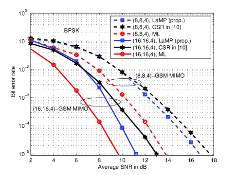
Figure 6: BER performance comparison between proposed LaMP detection, CSR detection in [10], and ML detection for $(8,8,4)$- and $(16,16,4)$-GSM MIMO.

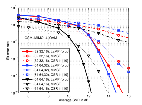
Figure 7: BER performance comparison between LaMP detection, CSR detection, and MMSE detection for $(32,32,16)$-, $(64,64,32)$- and $(64,64,16)$-GSM MIMO.

Simulation results: For comparison purposes, we simulated the detection performance of convex superset relaxation (CSR) based detection in [10] for GSM-MIMO. We have adapted the CSR algorithm presented for GSSK in [10] to GSM by modifying one of the CSR’s constraints, namely, $\sum_{i=1}^{N}x_{i}=R$ to $\|{\bf x}\|^{2}\leq R\gamma$, where $\gamma$ is the signal power of the modulation alphabet.

Figure 6 presents a performance comparison between the proposed LaMP detection, ML detection, and CSR based detection for different $(N,M,R)$- GSM MIMO systems with BPSK. It can be seen that the LaMP performance is away from ML performance by about 3 dB and 1.6 dB for $(8,8,4)$- and $(16,16,4)$-GSM MIMO systems, respectively, at $10^{-5}$ BER. Thus, the performance of LaMP improves as the system dimensions increase. Also, LaMP detection performs better than the CSR detection in [10] – e.g., by about 1.8 dB at $10^{-5}$ BER in $(16,16,4)$-GSM MIMO system. Figure 7 presents a performance comparison between the LaMP detection, MMSE detection (performed as $[{\bf H}^{H}{\bf H}+\frac{1}{SNR}{\bf I}]^{-1}{\bf H}^{H}{\bf y}$), CSR detection in [10] for the following large-scale GSM-MIMO system configurations: ($i$) $(32,32,16)$-GSM, 4-QAM, $|{\cal A}|=2^{29}$, $61$ bpcu, ($ii$) $(64,64,16)$-GSM, 4-QAM, $|{\cal A}|=2^{48}$, $80$ bpcu, and ($iii$) $(64,64,32)$-GSM, 4-QAM, $|{\cal A}|=2^{60}$, $124$ bpcu. It can be seen that the proposed LaMP algorithm performs better and its performance improves as the dimensionality of the GSM signal increases.

In Fig. 8, we plot the average SNR required by the LaMP detection algorithm to achieve a target BER of $10^{-3}$ as the number of receive antennas $M$ is varied. We consider two GSM MIMO systems here, ($i$) $N=32,R=16$, 4-QAM, $61$ bpcu, and ($ii$) $N=16,R=8$, 4-QAM, $29$ bpcu. From Fig. 8, it can be seen that as $M$ increases the SNR required to achieve the target BER reduces. It can also be observed that the LaMP detection algorithm performs well even when the system is underdetermined, i.e., $M<N$. This is because the LaMP detection algorithm exploits the sparse structure of the GSM transmit signals to efficiently perform detection.

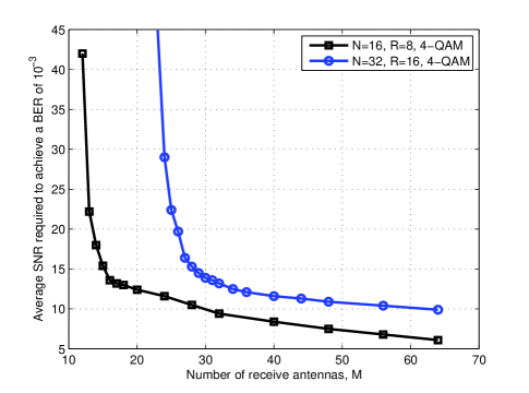
Figure 8: Average SNR required by the LaMP detection algorithm to achieve a BER of $10^{-3}$ as the number of receive antennas $M$ is varied for $N=32,R=16$, and $N=16,R=8$ GSM MIMO systems with 4-QAM.

V Conclusions

We studied GSM MIMO capacity and low complexity methods for GSM encoding and detection. We made the following key contributions in this paper: 1) we derived lower and upper bounds on the GSM MIMO capacity, 2) we proposed an efficient GSM encoding method using combinadics for large number of transmit antennas and RF chains, and 3) we also proposed a message passing based low-complexity detection algorithm suited for large-scale GSM MIMO systems.

References

- [1] M. Di Renzo, H. Haas, A. Ghrayeb, S. Sugiura, and L. Hanzo, “Spatial modulation for generalized MIMO: challenges, opportunities and implementation,” Proceedings of the IEEE, vol. 102, no. 1, Jan. 2014.
- [2] J. Wang, S. Jia, and J. Song, “Generalised spatial modulation system with multiple active transmit antennas and low complexity detection scheme,” IEEE Trans. Wireless Commun., vol. 11, no. 4, pp. 1605-1615, Apr. 2012.
- [3] T. Datta and A. Chockalingam, “On generalized spatial modulation,” Proc. IEEE WCNC’2013, Shanghai, Apr. 2013.
- [4] T. Lakshmi Narasimhan, P. Raviteja, and A. Chockalingam, “Large-scale multiuser SM-MIMO versus massive MIMO,” Proc. ITA’2014, San Diego, Feb. 2014.
- [5] T. Lakshmi Narasimhan, P. Raviteja, and A. Chockalingam, “Generalized spatial modulation in large-scale multiuser MIMO systems,” IEEE Trans. Wireless Commun., vol. 14, no. 7, pp. 3764-3779, Jul. 2015.
- [6] Y. Hou , P. Wang, W. Xiang, X. Zhao, and C. Hou, “Ergodic capacity analysis of spatially modulated systems,” China Commun., vol. 10, no. 7, pp. 118-125, Jul. 2013.
- [7] D. Tse and P. Viswanath, Fundamentals of Wireless Communication, Cambridge Univ. Press, 2005.
- [8] A. Chockalingam and B. Sundar Rajan, Large MIMO Systems, Cambridge Univ. Press, Feb. 2014.
- [9] D. E. Knuth, The Art of Computer Programming, Volume 4A: Combinatorial Algorithms, Pearson Education, 2011.
- [10] R. Y. Chang, W-H. Chung, and S-J. Lin, “Detection of space shift keying signaling in large MIMO systems,”Proc. IWCMC’2012, pp. 1185-1190, Aug. 2012.