Nuclear $\beta^{-}$-decay half-lives for $fp$ and $fpg$ shell nuclei

Abstract

In the present work we calculate the allowed $\beta^{-}$-decay half-lives of nuclei with $Z=20-30$ and N $\leq$ 50 systematically under the framework of the nuclear shell model. A recent study shows that some nuclei in this region belong to the island of inversion. We perform calculation for $fp$ shell nuclei using KB3G effective interaction. In the case of Ni, Cu, and Zn, we used JUN45 effective interaction. Theoretical results of $Q$ values, half-lives, excitation energies, log$ft$ values, and branching fractions are discussed and compared with the experimental data. In the Ni region, we also compared our calculated results with recent experimental data [Z. Y. Xu et al., Phys. Rev. Lett. 113, 032505, 2014]. Present results agree with the experimental data of half-lives in comparison to QRPA.

1 Introduction

The neutron density becomes very diffused and the single-particle spectrum shows the similarity of the harmonic-oscillator as we approach towards the neutron-drip line [1, 2]. We can see this effect at $N=40$ shell gap. Recently intruder configurations are found in the neutron rich nuclei around this shell gap [3, 4, 5, 6, 7]. Thus the nuclear structure study of these nuclei in this region is very important [8, 9, 10].

Sorlin et al. [11], observed the experimental beta decay half-lives of neutron rich ^57-59Ti, ^59-62V, ^61-64Cr, ^63-66Mn, ^65-68Fe and ^67-70Co isotopes around $N=40$ at GANIL. Sorlin et al., also compared experimentally observed half-lives of V and Cr isotopes with QRPA calculation. The QRPA calculations for ^58,59Cr, ^61-63Mn, ^63-64Fe, ^65-67Co and ^67,69Ni with folded-Yukawa single-particle potential are reported in ref. [12]. The authors of [12], have also compared the results with Bender et al., [13] based on Nilsson potential. Using RIBF facility at RIKEN, the half-lives of twenty neutron-rich nuclei with $Z=27-30$ are reported in ref. [14]. In that work, sizable magicity was reported for both the proton number $Z=28$ and the neutron number $N=50$ in ⁷⁸Ni. A sudden shortening of half-lives of the nickel isotopes beyond $N=50$ were observed in this work, although this effect is not found in the Cu-Ge-Ga chains. The half-lives results from LISE2000 spectrometer at GANIL for ⁷¹Co and ⁷³Co are reported in ref. [15]. The half-lives of ^77,78Ni were measured for the first time by Hosmer et al. [16], at NSCL, MSU. Recently the beta decay half-lives of 38 very neutron-rich Kr to Tc isotopes are measured at RIKEN [17].

Despite the progress in the experimental side, we need theoretical estimates for half-lives of neutron rich nuclei, especially those belonging to the island of inversion. These calculations are based on allowed GT-transitions. Many theoretical calculations from the quasiparticle random phase approximation (QRPA) based on the Hartree-Fock Bogoliubov theory [18] or other global models [19, 20, 21] are available in the literature. These calculations underestimate the correlation among nucleons which predict GT-strength at low-energies. Recently, shell model calculations for the $\beta^{-}$-decays of $Z=9-13$ nuclei are reported by Li and Ren [22]. The motivation of the present work is to study $\beta^{-}$-decay properties of $Z=20-30$ nuclei using the nuclear shell model.

This paper is organized as follows. In section 2, we present the formulas for the calculation of $\beta^{-}$ decay half-lives. Shell model spaces, effective interactions and the quenching factors adopted in our calculations are reported in section 3. In section 4, we present theoretical results along with the experimental data wherever available. Finally, summary and conclusions are drawn in section 5.

2 Formalism

In the beta decay, the transitions start from the ground state of the parent nuclei to different excited states (only those inside the energy window defined by $Q$-value) of the daughter nuclei according to the selection rule of beta – decay. The $ft$ value is calculated by

$$ft=\frac{6177}{[(g_{A})^{2}B(GT)+B(F)]}$$ (1)

where, $g_{A}$ (= 1.260) is the axial-vector coupling constant of the weak interactions. Here, $f$ is a phase-space integral that contains the lepton kinematics. The $B(GT)$ and $B(F)$ are the Gamow-Teller and Fermi matrix elements. The total half-life is calculated as

$$t_{1/2}=({\sum_{i}{\frac{1}{t_{i}}}})^{-1}$$ (2)

where $t_{i}$ is the partial decay half life of the daughter’s state i. The partial half-life of the allowed $\beta^{-}$-decay is given by [23],

$$t_{i}=10^{logft-logf_{A}}$$ (3)

here, ${f_{A}}$ is the Gamow -Teller (axial-vector) phase space factor. Because the $ft$ values are usually large, they are normally expressed in terms of ‘log $ft$ values’. The log $ft$ value is defined as log$ft$ $\equiv$ log${}_{10}(f_{A}t_{i}[s])$.

The partial half-life $t_{i}$ is related to the total half-life $t_{1/2}$ of the allowed $\beta^{-}$-decay as

$$t_{i}={\frac{t_{1/2}}{b_{r}}}$$ (4)

where, ${b_{r}}$ is the branching ratio for the level with partial half-life ${t_{i}}$. The $B(GT)$ is the Gamow-Teller matrix element

$$B(GT)=(\frac{g_{A}}{g_{V}})^{2}{\langle{\sigma\tau}\rangle}^{2}$$ (5)

The nuclear matrix element of Eqn. (5) for the Gamow-Teller operator is

$${\langle{\sigma\tau}\rangle}={\langle{f}||\sum_{k}{\sigma^{k}\tau_{\pm}^{k}}||i\rangle}/\sqrt{2J_{i}+1},$$ (6)

where $f$ and $i$ refer to all the quantum numbers needed to specify the final and initial states, respectively, $\pm$ refers to $\beta^{\pm}$ decay, $\tau_{\pm}=\frac{1}{2}(\tau_{x}+i\tau_{y})$ with $\tau_{+}p$ = $n$, $\tau_{-}n$ = $p$, and $J_{i}$ is the total angular momentum of the initial-state. The sum in Eqn. (6) runs over all the nucleons. We calculate the values of ${f_{A}}$ and ${\langle{\sigma\tau}\rangle}^{2}$ from the refs. [24, 25, 26].

We also report the $\beta$-decay $Q$ value using shell model calculations, the theoretical $\beta$-decay $Q$ value is given by

$$Q=(E(SM)_{i}+E(C)_{i})-(E(SM)_{f}+E(C)_{f})$$ (7)

where $E(SM)$ is the nuclear binding energy of the interaction of the valence particles among themselves, which can be evaluated from the shell model calculation, $E(C)$ is the valence space Coulomb energy, and subscripts $i$ and $f$ denote the parent and daughter nuclei, respectively. The expression for $E(C)$ is taken from ref. [27].

3 Hamiltonian and quenching factor

In the present work we performed calculation for $fp$ and $f_{5/2}pg_{9/2}$ shell nuclei using the shell model code NuShellX@MSU [28]. For $fp$ shell nuclei, we used KB3G effective interaction [29]. In the case of $f_{5/2}pg_{9/2}$ model space for Ni, Cu and Zn isotopes, we performed calculations with JUN45 effective interaction [30]. While NuShellX is a set of shell model computer codes written by Bill Rae [31], NuShellX@MSU is a set of wrapper codes written by Alex Brown. NushellX is based on OpenMP to use many cores with high efficiency for Lanczos interactions. NuShellX uses a proton-neutron basis. With NuShellX, it is possible to diagonalize J-scheme matix dimensions up to $\sim$ 100 million. The Hamiltonian is written as a sum of three terms $H=H_{nn}+H_{pp}+H_{pn}$. With this code it is possible to calculate spectroscopic factors, two-nucleon transfer amplitudes and one-body transition densities. In the DENS program, it is possible to use radial wavefunctions from harmonic-oscillator, Woods-Saxon or Skyrme-density functions methods for the matrix elements. With the NushellX code it is possible to calculate log$ft$ values and $GT$ strength to individual final states but not the total strength. The parameters which we need for the calculations are the model space and the corresponding effective interaction (two-body matrix elements).

We performed calculation for nuclei in two different model spaces. Thus we used two different effective interactions JUN45 and KB3G. The KB3G [29] interaction is extracted from the KB3 interaction by introducing mass dependence and refining its original monopole changes in order to treat properly the $N=Z=28$ shell closure and its surroundings. In order to recover simultaneously the good gaps around ⁴⁸Ca and ⁵⁶Ni, here $T=0$ and $T=1$ modifications are different. The single-particle energies for KB3G effective interaction are taken to be -8.6000, -6.6000, -4.6000 and -2.1000 MeV for the $f_{7/2}$, $p_{3/2}$, $p_{1/2}$ and $f_{5/2}$ orbits, respectively.

The JUN45 effective interaction, which was recently developed by Honma [30], is a realistic interaction based on the Bonn-C potential fitting by 400 experimental binding and excitation energy data with mass numbers A = 63 - 96. For the JUN45 interaction, the single-particle energies are taken to be -9.8280, -8.7087, -7.8388 and -6.2617 MeV for the $p_{3/2}$, $f_{5/2}$ , $p_{1/2}$ and $g_{9/2}$ orbits, respectively. The large number of experimental data around $N=50$ shell closure has been taken for the fitting of this interaction. For this interaction an rms deviation is 185 keV. We performed full-fledged calculation, but for few $fp$ shell nuclei we freeze 2 - 8 neutrons in the $f_{7/2}$ orbital.

Following Ref. [32] we can define matrix elements, $M(GT)$, in terms of reduced transition probability, $B(GT)$, by following

$$M(GT)=[(2J_{i}+1)B(GT)]^{1/2},$$ (8)

this is independent of the direction of the transitions. Here $J_{i}$ is the total angular momentum of the initial state. To get effective $g_{A}$, first we normalize the $M(GT)$ to the “expected” total strength W, defined by

$$W=\left\{\begin{array}[]{@{}ll@{}}|g_{A}/g_{V}|[(2J_{i}+1)3|N_{i}-Z_{i}|]^{1/2},&forN_{i}\neq Z_{i},\\ |g_{A}/g_{V}|[(2J_{f}+1)3|N_{f}-Z_{f}|]^{1/2},&forN_{i}=Z_{i},\end{array}\right.$$ (9)

The matrix elements $R(GT)$ are defined as

$$R(GT)=M(GT)/W.$$ (10)

The comparison of the experimental versus the theoretical $R(GT)$ values are plotted in Fig. 1. The $R(GT)_{exp}$ values are taken from the experimental log$ft$ values (as given in the table 1).

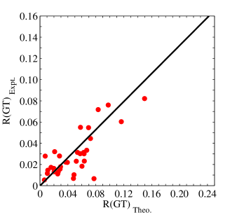
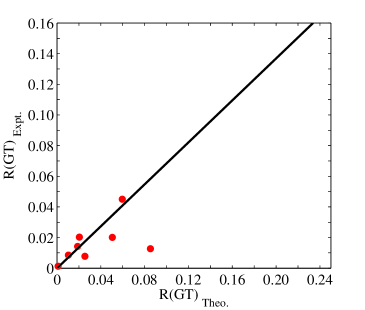
Figure 1: Comparison of the experimental matrix element $R(GT)$ values with theoretical calculations based on the “free-nucleon” Gamow-Teller operator. Each transition is indicated by a point in the x-y plane. Theoretical and experimental value given by the x, y coordinates, respectively. Left panel for $fp$ model space with KB3G effective interaction, while the right panel for $f_{5/2}pg_{9/2}$ model space with JUN45 effective interaction.

The quenching factor is defined as the square root of the ratio of the experimental measured rate to the calculated rate in a full $0\hbar\omega$ calculation. Because the observed Gamow-Teller strength appears to be systematically smaller than what is theoretically expected on the basis of model independent Ikeda sum rule “3(N-Z)”. The quenching factor $q$ in a given model space is obtained by averaging all the ratios between the experimental and theoretical $R(GT)$ values. The points follow nicely a straight line whose slope gives the average quenching factor. In the present work we performed the shell model calculations for two different model spaces. Thus, we have two different quenching factors. From this work for $pf$ shell nuclei we have $q$ = 0.660 $\pm$ 0.016, while for $f_{5/2}pg_{9/2}$ shell nuclei we have $q$ = 0.684 $\pm$ 0.015.

Table 1: Comparisons of the theoretical log$ft$ values, excitation energies, and branching percentages of $\beta$-decays of the concerned nuclei with the experimental values. An asterisk beside the experimental excitation energy indicates that the experimental $J^{\pi}$ of this state is uncertain. References to the experimental data are given in the last column.

			Ex. energy (keV)			log$ft$ value			Branching ($\%$)
AZ${}_{i}(J^{\pi})$	AZ${}_{f}(J^{\pi})$		Theo.	Expt.		Theo.	Expt.		Theo.	Expt.		Ref.
52Ca($0^{+}$)	52Sc($1^{+}$)		1306	1636		4.309	5.07		93.81	86.8		[33]
			2606	4266		4.997	5.8		6.19	1.4
54Ca($0^{+}$)	52Sc($1^{+}$)		0	247		3.921	4.25		89.25	97.17		[34]
54Sc($3^{+}$)	54Ti($4^{+}$)		2452	2497		5.173	5.3		50.26	33		[35]
	54Ti($2^{+}$)		1285	1495		5.731	5.7		22.53	21
55Sc($7/2^{-}$)	55Ti($9/2^{-}$)		1562	2146		4.660	5.3		10.84	11		[35]
	55Ti($7/2^{-}$)		1079	1796		4.341	5.0		28.09	22
	55Ti($5/2^{-}$)		0	592		4.202	5.0		61.1	39
57Ti($5/2^{-}$)	57V($7/2^{-}$)		161	175*		4.259	5.7$\pm$0.2		51.28	5$\pm$3		[36]
			1836	1754*		6.806	4.9$\pm$0.2		0.06	16$\pm$2
			2328	2476*		4.654	5.0$\pm$0.2		6.75	7.3$\pm$0.7
	57V($3/2^{-}$)		1711	1732*		5.141	6.0$\pm$0.2		3.11	1.1$\pm$0.7
			2040	2036*		5.499	4.8$\pm$0.2		1.14	16$\pm$2
56V($1^{+}$)	56Cr($2^{+}$)		920	1006		5.477	5.63		2.67	$<$4		[37]
			1705	1830		5.103	6.01		3.95	1.0
			2178	2324		5.384	5.87		1.53	1.0
	56Cr($0^{+}$)		0	0		4.399	4.62		52.22	70
			1463	1675		4.242	4.63		33.30	26
57V($3/2^{-}$)	57Cr($5/2^{-}$)		195	268*		5.404	4.67		7.25	47		[37]
			692	693*		8.785	4.93		0.002	20
			1616	1583*		6.814	5.51		0.11	3
58V($1^{+}$)	58Cr($2^{+}$)		731	879		4.047	$>$5.3		44.2	$<$34		[38]
	58Cr($0^{+}$)		0	0		4.089	$>$5.3		54.65	$<$38
60Cr($0^{+}$)	60Mn($1^{+}$)		0	0		3.485	4.2$\pm$0.1		95.26	88.6$\pm$0.6		[39]
			1120	759		4.469	5.0$\pm$0.2		4.14	5.0$\pm$0.5
61Cr($5/2^{-}$)	61Mn($7/2^{-}$)		185	157		4.887	5.6$\pm$0.1		13.62	9$\pm$2		[40]
	61Mn($5/2^{-}$)		1645	1497*		6.484	4.9$\pm$0.2		0.15	20$\pm$5
			2098	2032*		4.356	5.4$\pm$0.2		15.46	5$\pm$1
	61Mn($3/2^{-}$)		866	1142*		5.559	5.6$\pm$0.4		2.01	5$\pm$4
			1623	1860*		7.026	4.8$\pm$0.1		0.045	20$\pm$2
62Cr($0^{+}$)	62Mn($1^{+}$)		579	0		3.782	$\sim$4.2		43.78	$\sim$72		[41]
			823	640		3.631	$\sim$4.4		56.14	$\sim$25
			1794	1500*		6.291	5.3		0.08	3

Table 1: Continuation.

			Ex. energy (keV)			log$ft$ value			Branching ($\%$)
AZ${}_{i}(J^{\pi})$	AZ${}_{f}(J^{\pi})$		Theo.	Expt.		Theo.	Expt.		Theo.	Expt.		Ref.
60Mn($1^{+}$)	60Fe($2^{+}$)		658	823		4.866	5.6$\pm$0.2		7.35	4.2$\pm$1.2		[42]
	60Fe($0^{+}$)		0	0		4.070	4.46$\pm$0.04		66.98	88$\pm$2		[42]
			1345	1974		4.242	5.15$\pm$0.07		20.15	5.0$\pm$0.6
			2291	2356		4.860	5.3$\pm$0.1		2.51	3.0$\pm$0.5
61Mn($5/2^{-}$)	61Fe($7/2^{-}$)		991	960		5.995	6.6(1)		0.35	0.49(7)		[43]
			1906	1929*		7.532	5.40(2)		0.05	2.7(1)
			2120	2144*		5.990	5.43(2)		0.14	1.8(1)
	61Fe($5/2^{-}$)		243	207		4.575	5.38(13)		15.95	12.6(8)		[43]
			1149	1161		5.681	5.64(1)		0.65	3.25(7)
	61Fe($3/2^{-})$		0	0		4.052	5.02(3)		62.25	33(1)		[43]
			831	629		4.291	4.77(1)		20.36	39.0(6)
			1464	1253		6.892	6.4(5)		0.03	0.57(6)
62Mn($4^{+}$)	62Fe($5^{+}$)		3719	3714*		5.629	$>$6.4		1.11	1.2		[44]
	62Fe($4^{+}$)		2111	2177		5.788	5.9		2.17	8.4		[44]
	62Fe($3^{+}$)		2357	2692		4.274	5.5		61.11	17		[44]
			3384	3360*		7.436	$>$6.5		0.02	1.2
64Mn($1^{+}$)	64Fe($2^{+}$)		1424	1444*		4.705	$\sim$5.6		15.52	$\sim$7.3		[45]
	64Fe($1^{+}$)		3384	3307*		4.070	$\sim$5.5		25.66	$\sim$4.0
			3910	4227*		5.742	$\sim$5.7		0.40	$\sim$1.4
73Ni($9/2^{+}$)	73Cu($9/2^{+}$)		1812	1489		5.062	$>$5.8		25.61	$<$15.7		[46]
	73Cu($7/2^{+}$)		1423	961		4.866	$>$5.9		40.02	$<$19.2
76Cu($3^{+}$)	76Zn($4^{+}$)		1641	1296		5.769	5.8		11.78	24(4)		[47]
			1814	2633*		5.467	5.9		21.99	10(2)
			2666	2814*		6.669	6.3		0.95	3.8(7)
	76Zn($3^{+}$)		1788	3232*		5.191	6.0		21.51	6.2(12)
			2107	3273*		5.689	6.5(3)		11.64	1.7(10)
	76Zn($2^{+}$)		2244	2266*		6.370	6.3(1)		2.28	4.9(13)
			2540	2349*		5.870	8(4)		6.34	0.1(9)
77Cu($5/2^{-}$)	77Zn($5/2^{-}$)		1104	1284*		5.889	6.5		4.53	2		[48]
			1813	2082*		6.003	6.1		2.64	3
78Cu($5^{-}$)	78Zn($6^{-}$)		3732	3105		6.035	5.5(1)		13.09	21(3)		[49]
79Zn($9/2^{+}$)	79Ga($11/2^{+}$)		2644	2561*		5.054	$\geq$6.3		28.07	$\leq$2		[50]
			2656	2649*		5.830	5.9		4.67	4.0
			2846	2919*		3.782	5.7		12.93	5.6
	79Ga($9/2^{+}$)		2785	2741*		5.755	5.4		5.93	13
	79Ga($7/2^{+}$)		3105	3020*		6.788	5.5		0.54	7.4
80Zn($0^{+}$)	80Ga($1^{+}$)		617	686		3.746	5.6		75.99	5.5		[51]
			844	965		4.202	5.2		23.12	10.1
			1487	1504		5.444	5.6		0.87	3.1
			1674	2070		7.551	4.5		0.006	20.5

4 Results and discussions

The comparison between theoretical and experimental log$ft$ values, excitation energies, and the branching percentages of $\beta$-decays of the concerned nuclei are shown in the table 1. The theoretical and experimental excitation energies of each state involved in the $\beta$ - decays are listed in column 3 and 4, respectively. The theoretical and experimental log$ft$ values are listed in column 5 and 6, respectively. The branching fractions are given by $b_{r}=t_{1/2}/t_{i}$, where $t_{1/2}$ is the nuclear $\beta$ - decays half life and $t_{i}$ is the partial half-life of each transition. The theoretical branching fractions are listed in column 7 and the experimental values are listed in column 8. In this table, we present experimental uncertain state by ‘*’. The shell model results for $fp$ and $f_{5/2}pg_{9/2}$ shell nuclei are showing a good agreement with the experimental data for excitation energies, log$ft$ values and the branching ratios.

In the table 2, we compare the theoretical and the experimental $\beta$-decay half-lives of the concerned nuclei. The experimental $Q$ values, $\beta^{-}$-decay probabilities and the quenched theoretical sum $B(GT)$ values are also reported in this table. The first and second columns are the parent and daughter nuclei, respectively. Column 3 presents the experimental $Q$ values, which are taken from [52]. In column 4 we present the sums of quenched $B(GT)$ values. Theoretical and experimental $\beta$-decays half-lives are presented in columns 5 and 6, respectively. In the last column we present the experimental probabilities of $\beta^{-}$-decay. The probabilities of $\beta^{-}$-decay for most of the nuclei are 100%. In this table, we present the experimental value which is unknown by ’?’. We determined the ground states using the shell model for the nuclei where the experimental ground states are not confirmed. In these cases we calculate the $\beta$-decay properties for the three lowest states as reported in table 1.

The ^63-65Mn nuclei belong to the island of inversion [5]. The experimental $\beta^{-}$-decay half-lives for these three nuclei are 275 $\pm$ 4 ms, 90 $\pm$ 4 ms, and 84 $\pm$ 8 ms, respectively, while the calculated shell model results are 216 ms, 61 ms and 73 ms, respectively. The calculations are remarkably close to the measured values. We also reported the calculated $\beta^{-}$-decay half-lives for some nuclei such as ^57-58Ca, ^59-61Sc, and ⁶²Ti, where exact experimental values are still not known.

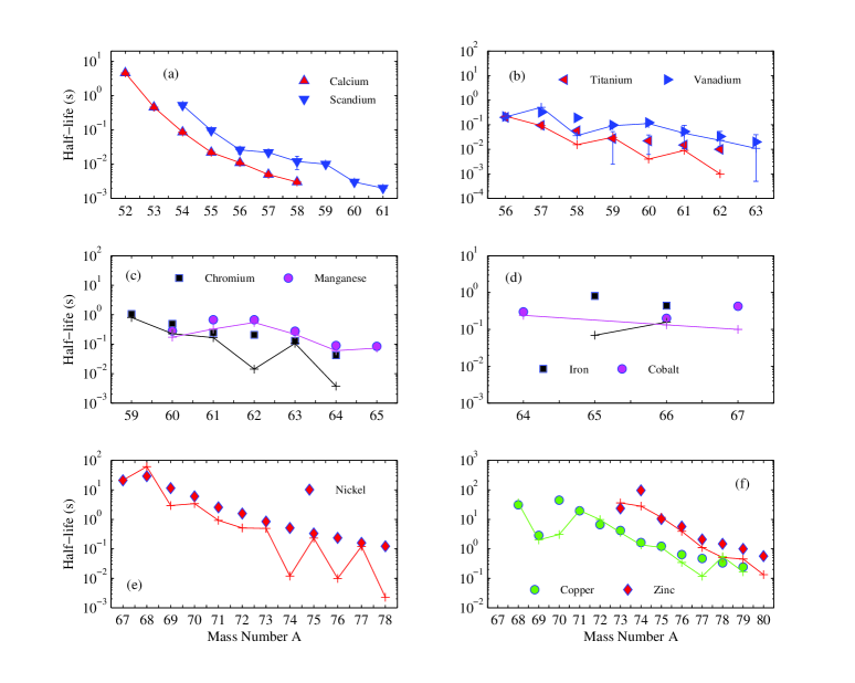
Figure 2: The $\beta$-decay half-life versus the mass number A of the concerned nuclei. The experimental results are represented by points with error bars while the theoretical results are represented by solid lines with ‘+’ sign. The nuclei are grouped by proton number $Z$.

In the Fig. 2, we show the theoretical and experimental $\beta$-decay half-lives of concerned nuclei taken from table 2. We used the log frame to show $\beta$-decay half-lives. Here, the $\beta$-decay half-lives decrease rapidly with the increasing neutron number. In this figure we presented the experimental data with error bars while the theoretical results are connected by solid lines with ‘+’ sign. In the case of most $fp$ shell nuclei results are in a good agreement with experimental data. For a few heavier even-even $fp$ shell nuclei (around $\sim N=40$), the calculated results are not in a good agreement with the experimental data. This may be due to the missing $\nu d_{5/2}$ orbital in the model space. The results with JUN45 interaction is showing a good agreement for Ni, Cu and Zn isotopes, except for 3 even-even Ni nuclei. We take new experimental results of half-lives from ref. [14] for comparison with the calculated values. Our results are closer to the experimental data in comparison to previously available QRPA results in ref. [19], because GT-strength is underestimated in QRPA. Some of the concerned nuclei belong to the island of inversion, such as $\mathrm{{}^{63-65}Mn}$ and $\mathrm{{}^{67}Co}$, and their $\beta$-decays properties are well reproduced by our calculations.

The theoretical result shows better agreement with the experimental data for a relatively small neutron number. As we move towards drip line, some of the theoretical results deviate from the experimental data. This is because our calculations are unable to predict the ground state correctly, and uncertainties of the $Q$ values are large. These facts are responsible for the large errors of the theoretical half-lives.

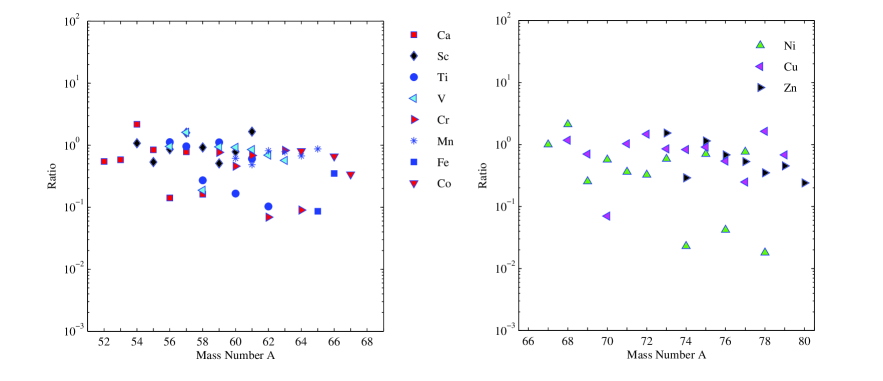
Figure 3: The ratios of theoretical to experimental half-lives versus the mass number $A$ for the concerned nuclei.

From the table 2, we also show the ratios between theoretical $\beta$-decay half-lives and experimental data for the concerned nuclei in Fig. 3. Here, in the left figure we shown the results for $fp$ shell nuclei using KB3G effective interaction, while in the right figure we shown the results of Ni, Cu and Zn isotopes using JUN45 effective interaction.

We also report the $\beta$-decay $Q$ values using Eqn. (7) and compare with the experimental data in table 3. Although we are not using these theoretical $Q$ values for the evaluation of $\beta$-decays half-lives as reported in table 1. We take the experimental data from ref. [52] ( where ‘#’ indicates that the presented value is estimated from systematic trends). The rms deviation between theory and experiment is 1162 keV.

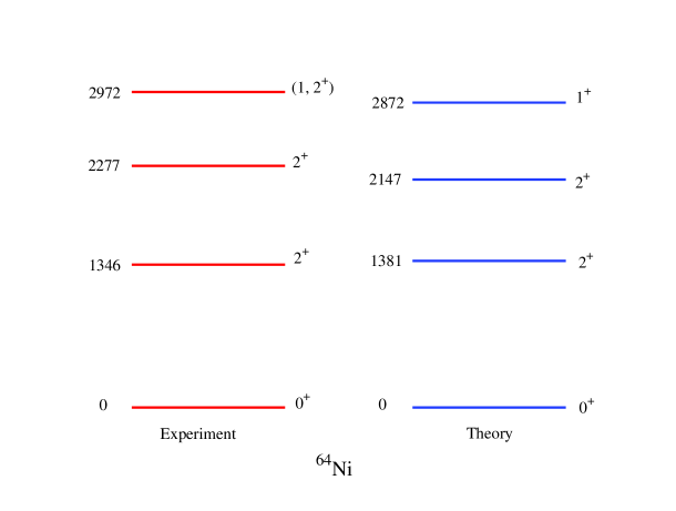
Figure 4: Comparison of the theoretical and experimental energy levels of ⁶⁴Ni.

In the Fig. 4, we show the comparison between the calculated and the experimental energy levels for ⁶⁴Ni. In the case of ⁶⁴Co and ⁶⁴Ni, we performed calculation in $fp$ model space using KB3G effective interaction. Here we put minimum 6 and 4 particles in $\pi f_{7/2}$ and $\nu f_{7/2}$ orbitals, respectively. The energy levels are in a good agreement with the experimental data. The calculated partial half-life for $2_{1}^{+}$ to $0_{1}^{+}$ transition is 1.0 $ps$ while corresponding experimental value is 1.088 $ps$. The calculated partial half-life for $2_{2}^{+}$ to $0_{1}^{+}$ transition is 1.11 $ps$, although for this transition experimental data is not available.

Table 2: Comparison of the theoretical $\beta$-decay half-lives with the experimental data for the concerned nuclei together with the experimental $Q$ values [52], $\beta^{-}$-decay probabilities and quenched theoretical sum $B(GT)$ values.

		$Q$ value	Sum	Half-life			$\beta^{-}$
AZ${}_{i}(J^{\pi})$	AZf	(keV)	$B(GT)$	Theo.	Expt.		$\%$
52Ca($0^{+}$)	52Sc	5900	0.1004	2.519 s	4.6$\pm$0.3 s[53]		100
53Ca($1/2^{-}$)	53Sc	9650#	0.140	268.87 ms	461$\pm$90 ms[53]		100
54Ca($0^{+}$)	54Sc	8820#	0.895	186.7 ms	86$\pm$7 ms[53]		100
55Ca($5/2^{-}$)	55Sc	16630#	0.0902	18.51 ms	22$\pm$2 ms[53]		100
56Ca($0^{+}$)	56Sc	10830#	0.799	1.56 ms	11$\pm$2 ms[53]		100
57Ca($5/2^{-}$)	57Sc	13830#	0.322	3.90 ms	5 ms($>$620 ns)[53]		?
58Ca($0^{+}$)	58Sc	12960#	1.386	0.486 ms	3 ms($>$620 ns)[53]		?
54Sc($3^{+}$)	54Ti	12000	0.023	565.7 ms	526$\pm$15 ms[53]		100
55Sc($7/2^{-}$)	55Ti	11690	0.221	51.30 ms	96$\pm$2 ms[53]		100
56Sc($1^{+}$)	56Ti	14470#	0.489	22.37 ms	26$\pm$6 ms[53]		100
57Sc($7/2^{-}$)	57Ti	13160#	0.068	34.93 ms	22$\pm$2 ms[53]		100
58Sc($3^{+}$)	58Ti	16240#	0.269	11.03 ms	12$\pm$5 ms[53]		100
59Sc($7/2^{-}$)	59Ti	15340#	0.380	5.10 ms	10 ms($>$620 ns)[53]		?
60Sc($3^{+}$)	60Ti	18280#	0.935	2.35 ms	3 ms($>$620 ns)[53]		?
61Sc($7/2^{-}$)	61Ti	17280#	0.388	3.31 ms	2 ms($>$620 ns)[53]		?
56Ti($0^{+}$)	56V	6920	0.661	224.5 ms	200$\pm$5 ms[53]		100
57Ti($5/2^{-}$)	57V	10360	0.306	91.1 ms	95$\pm$6 ms[53]		100
58Ti($0^{+}$)	58V	9210#	0.329	15.50 ms	57$\pm$10 ms[54]		100
59Ti($5/2^{-}$)	59V	12190#	0.1025	30.66 ms	27.5$\pm$25 ms[54]		100
60Ti($0^{+}$)	60V	10910#	0.586	3.697 ms	22.2$\pm$25 ms[54]		100
61Ti($1/2^{-}$)	61V	14160#	0.207	9.07 ms	15$\pm$4 ms[53]		100
62Ti($0^{+}$)	62V	12910#	1.138	1.029 ms	10 ms($>$620 ns)[53]		100
56V($1^{+}$)	56Cr	9160	0.230	206.32 ms	216$\pm$4 ms[53]		100
57V($3/2^{-}$)	57Cr	8300	0.476	513.7 ms	320$\pm$3 ms[54]		100
58V($1^{+}$)	58Cr	9210#	0.230	36.08 ms	191$\pm$10 ms[53]		100
59V($5/2^{-}$)	59Cr	10060	0.512	91.092 ms	97$\pm$2 ms[54]		100
60V($3^{+}$)	60Cr	13260	0.049	112.71 ms	122$\pm$18 ms[53]		100
61V($3/2^{-}$)	61Cr	14160#	0.512	44.95 ms	52.6$\pm$42 ms[54]		100
62V($3^{+}$)	62Cr	15420#	0.214	23.128 ms	33.5$\pm$20 ms[53]		100
63V($7/2^{-}$)	63Cr	13730#	0.343	10.89 ms	19.2$\pm$24 ms[54]		100
59Cr($1/2^{-}$)	59Mn	7630	0.076	805.5 ms	1050$\pm$90 ms[53]		100
60Cr($0^{+}$)	60Mn	6460	0.623	225.23 ms	490$\pm$10 ms[53]		100
61Cr($5/2^{-}$)	61Mn	9290	0.490	166 ms	243$\pm$11 ms[53]		100
62Cr($0^{+}$)	62Mn	7590#	0.678	14.25 ms	206$\pm$12 ms[53]		100
63Cr($1/2^{-}$)	63Mn	11160	0.098	106.5 ms	129$\pm$2 ms[53]		100
64Cr($0^{+}$)	64Mn	9530#	1.447	3.734 ms	42$\pm$2 ms[54]		100
60Mn($1^{+}$)	60Fe	8444	0.308	171.73 ms	280$\pm$20 ms[53]		100
61Mn($5/2^{-}$)	61Fe	7178	0.291	325.50 ms	670$\pm$40 ms[53]		100

Table 2: Continuation.

		$Q$ value	Sum	Half-life			$\beta^{-}$
AZ${}_{i}(J^{\pi})$	AZf	(keV)	$B(GT)$	Theo.	Expt.		$\%$
62Mn($1^{+}$)	62Fe	10400#	0.391	952.6 ms	92$\pm$13 ms[53]		100
63Mn($5/2^{-}$)	63Fe	8749	0.368	216.1 ms	275$\pm$4 ms[53]		100
64Mn($1^{+}$)	64Fe	11981	0.271	60.53 ms	90$\pm$4 ms[14]		100
65Mn($5/2^{-}$)	65Fe	10254	0.436	73.21 ms	84$\pm$8 ms[14]		100
65Fe($1/2^{-}$)	65Co	7964	0.880	69.59 ms	810$\pm$50 ms[53]		100
66Fe($0^{+}$)	66Co	6341	1.105	157.2 ms	440$\pm$60 ms[14]		100
64Co($1^{+}$)	64Ni	7307	0.3481	241.8 ms	300$\pm$30 ms[53]		100
66Co($1^{+}$)	66Ni	9598	0.300	132.35 ms	200$\pm$2 ms[14]		100
67Co($7/2^{-}$)	67Ni	8421	0.467	99.98 ms	425$\pm$20 ms[14]		100
67Ni($1/2^{-}$)	67Cu	3576	0.081	21.19 s	21$\pm$1 s [53]		100
68Ni($0^{+}$)	68Cu	2103	1.079	61.32 s	29$\pm$2 s[53]		100
69Ni($9/2^{+}$)	69Cu	5758	0.068	2.93 s	11.5$\pm$0.3 s [53]		100
70Ni($0^{+}$)	70Cu	3763	0.670	3.42 s	6.0$\pm$0.3 s[53]		100
71Ni($9/2^{+}$)	71Cu	7305	0.074	0.93 s	2.56$\pm$0.03 s [53]		100
72Ni($0^{+}$)	72Cu	5557	0.674	0.51 s	1.57$\pm$0.05 s[53]		100
73Ni($9/2^{+}$)	73Cu	8879	0.056	491.6 ms	840$\pm$30 ms [53]		100
74Ni($0^{+}$)	74Cu	7550#	0.545	11.93 ms	507.7$\pm$4.6 ms[14]		100
75Ni($7/2^{+}$)	75Cu	10230#	0.017	231.28 ms	331.6$\pm$3.2 ms[14]		100
76Ni($0^{+}$)	76Cu	9370#	0.282	9.904 ms	234.6$\pm$2.7 ms[14]		100
77Ni($9/2^{+}$)	77Cu	11770#	0.018	121.578 ms	158.9$\pm$4.2 ms[14]		100
78Ni($0^{+}$)	78Cu	10370#	0.870	2.255 ms	122.2$\pm$5.1 ms[53]		100
68Cu($1^{+}$)	68Zn	4440	0.077	36.12 s	30.9$\pm$0.6 s[53]		100
69Cu($3/2^{-}$)	69Zn	2681	0.043	2.0 m	2.85$\pm$0.15 m[53]		100
70Cu($6^{-}$)	70Zn	6588	0.035	3.05 s	44.5$\pm$0.2 s[53]		100
71Cu($3/2^{-}$)	71Zn	4618	0.029	19.9 s	19.4$\pm$1.4 s[53]		100
72Cu($2^{-}$)	72Zn	8363	0.037	9.8 s	6.63$\pm$0.03 s[53]		100
73Cu($3/2^{-}$)	73Zn	6606	0.035	3.58 s	4.2$\pm$0.3 s[53]		100
74Cu($2^{-}$)	74Zn	9751	0.013	1.36 s	1.63$\pm$0.05 s[53]		100
75Cu($5/2^{-}$)	75Zn	8088	0.057	1.11 s	1.22$\pm$0.003 s[53]		100
76Cu($3^{-}$)	76Zn	11327	0.031	344.75 ms	637.7$\pm$5.5 ms[53]		100
77Cu($5/2^{-}$)	77Zn	10280#	0.058	116.47 ms	467.9$\pm$2.1 ms[53]		100
78Cu($6^{-}$)	78Zn	12990	0.011	541.4 ms	330.7$\pm$2.0 ms[14]		100
79Cu($5/2^{-}$)	79Zn	11530#	0.019	164.3 ms	241.3$\pm$2.1 ms[14]		100
73Zn($1/2^{-}$)	73Ga	4106	0.296	36.14 s	23.5$\pm$1 s[53]		100
74Zn($0^{+}$)	74Ga	2293	0.416	27.9 s	95.6$\pm$1.2 s[53]		100
75Zn($7/2^{+}$)	75Ga	5906	0.019	11.70 s	10.2$\pm$0.2 s[53]		100
76Zn($0^{+}$)	76Ga	3994	0.264	3.93 s	5.7$\pm$0.3 s[53]		100
77Zn($7/2^{+}$)	77Ga	7203	0.068	1.10 s	2.08$\pm$0.05 s[53]		100
78Zn($0^{+}$)	78Ga	6223	0.267	0.51 s	1.47$\pm$0.15 s[53]		100
79Zn($9/2^{+}$)	79Ga	9115.4	0.056	450.88 ms	995$\pm$19 ms[53]		100
80Zn($0^{+}$)	80Ga	7575	0.417	133.1 ms	562.2$\pm$3.0 ms[14]		100

Table 3: Comparison of the theoretical $\beta$-decay $Q$ values with the experimental data. The experimental data are taken from [52] where $`{\#}^{\prime}$ indicates that the presented value is estimated from systematic trends.

$Q$ value (keV)				$Q$ value (keV)				$Q$ value (keV)
Nuclei	Theo.	Expt.		Nuclei	Theo.	Expt.		Nuclei	Theo.	Expt.
52Ca	5795	5900$\pm$140		53Ca	9055	9650$\pm$480#		54Ca	9432	8820$\pm$620#
55Ca	11867	11630$\pm$680#		56Ca	11829	10830$\pm$720#		57Ca	14308	13830$\pm$780#
58Ca	13934	12960$\pm$920#		54Sc	10634	12000$\pm$380		55Sc	10545	11690$\pm$490
56Sc	13191	14470$\pm$420#		57Sc	12969	13160$\pm$560#		58Sc	15194	16240$\pm$720#
59Sc	14644	15340$\pm$720#		60Sc	17203	18280$\pm$860#		61Sc	16426	17280$\pm$1000#
56Ti	6752	6920$\pm$200		57Ti	9615	10360$\pm$330		58Ti	9413	9210$\pm$420#
59Ti	11996	12190$\pm$430#		60Ti	11672	10910$\pm$550#		61Ti	14151	14160$\pm$1080#
62Ti	13631	12910$\pm$760#		56V	7856	9160$\pm$180		57V	7320	8300$\pm$230
58V	10667	9210$\pm$240		59V	10206	10060$\pm$290		60V	12581	13260$\pm$310
61V	12311	14160$\pm$900#		62V	14801	15420$\pm$330#		63V	14182	13730$\pm$610#
59Cr	5903	7630$\pm$240		60Cr	5569	6460$\pm$210		61Cr	9480	9290$\pm$130
62Cr	9184	7590$\pm$210#		63Cr	11779	11160$\pm$460		64Cr	11381	9530$\pm$300#
60Mn	6632	8444$\pm$4		61Mn	5646	7178$\pm$3		62Mn	8768	10400$\pm$150#
63Mn	9934	8749$\pm$6		64Mn	12181	11981$\pm$6		65Mn	11650	10254$\pm$8
65Fe	8789	7964$\pm$7		73Ni	7799	8879$\pm$3		74Ni	5670	7550$\pm$400
75Ni	9083	10230$\pm$300#		76Ni	7170	9370$\pm$500#		77Ni	10460	11770$\pm$530#
78Ni	8465	10370$\pm$950#		76Cu	10380	11327$\pm$7		77Cu	8223	10280$\pm$150#
78Cu	11531	12990$\pm$500#		79Cu	9365	11530$\pm$400#		79Zn	8132	9115.4$\pm$2.9
80Zn	6192	7575$\pm$4

5 Summary

In the present work, we reported the half-lives, log$ft$ values, and branching fractions of nuclei with $Z=20-30$ and N $\leq$ 50 using the nuclear shell model. We performed the calculation for $fp$ shell nuclei using KB3G effective interaction. In the case of Ni, Cu and Zn for $f_{5/2}pg_{9/2}$ model space we used JUN45 effective interaction. The comparison with experimental results of excitation energies, log$ft$ values, half-lives, $Q$-values and branching fractions for most of nuclei show a good agreement with the available experimental data. Some of the concerned nuclei belong to the island of inversion, such as $\mathrm{{}^{63-66}Mn}$ and $\mathrm{{}^{67}Co}$, and their $\beta$-decays are well reproduced by the calculations. The present shell model results will add more information to the earlier QRPA results [19]. The QRPA results for half-lives are larger because it is pushing down GT-strength at low energies. Further experimental half-lives measurement for very neutron-rich $fp$ and $f_{5/2}pg_{9/2}$ shell nuclei are strongly desired to test shell model effective interaction.

References

References

- [1] Dobaczewski J et al., 1994 Phys. Rev. Lett. 72 981.
- [2] Brown B A, 2001 Nucl. Phys. A 682 183c.
- [3] Ljungvall J et al., 2010 Phys. Rev. C 81 061301.
- [4] Recchia F et al., 2012 Phys. Rev. C 85 064305.
- [5] Naimi S et al., 2012 Phys. Rev. C 86 014325.
- [6] Tarasov O B et al., 2009 Phys. Rev. Lett. 102 142501.
- [7] Santamaria C et al., 2015 Phys. Rev. Lett. 115 192501.
- [8] Brown B A, 2010 Physics 3 104.
- [9] Lenzi S M , Nowacki F, Poves A, and Sieja K, 2010 Phys. Rev. C 82 054301.
- [10] Caurier E, Nowacki F, and Poves A, 2014 Phys. Rev. C 90 014302.
- [11] Sorlin O et al., 1999 Nucl. Phys. A 660, 3.
- [12] Möller P and Randrup J, 1990 Nucl. Phys. A 514, 1.
- [13] Bender E, Muto K and Klapdor H V et al., 1988 Phys. Lett. B 208, 53.
- [14] Xu Z Y et al., 2014 Phys. Rev. Lett. 113 032505.
- [15] Sawicka M et al., 2004 Eur. Phys. J. A 22 455.
- [16] Hosmer P T et al., 2005 Phys. Rev. Lett. 94 112501.
- [17] Nishimura S et al., 2011 Phys. Rev. Lett. 106 052502.
- [18] Engel J et al., 1999 Phys. Rev. C 60 014302.
- [19] Möller P et al., 1997 At. Data Nucl. Data Tables 66 131.
- [20] Möller P et al., 2003 Phys. Rev. C 67 055802.
- [21] Borzov I N et al., 1997 Nucl. Phys. A 621 307c.
- [22] Li Hantao and Ren Z, 2013 J. Phys. G: Nucl. Part. Phys. 40 105110.
- [23] Suhonen J, From Nucleons to Nucleus: Concepts of Microscopic Nuclear Theory (Springer, Berlin, 2007).
- [24] Wilkinson D H et al., 1973 Nucl. Phys. A 209 470.
- [25] Wilkinson D H , and Macefield B E F 1974 Nucl. Phys. A 232 58.
- [26] Wildenthal D H , Gallman A , and Alburger D E 1978 Phys. Rev. C 81 401.
- [27] Caurier E et al., 1999 Phys. Rev. C 59 2033.
- [28] Brown B A, Rae W D M, McDonald E, and Horoi M, NushellX@MSU.
- [29] Poves A et al., Nucl. Phys. A 694, 157 (2001).
- [30] Honma M, Otsuka T, Mizusaki T and Hjorth-Jensen M, 2009 Phys. Rev. C 80 064323.
- [31] Rae W D M, NuShellX.
- [32] Brown B A and Wildenthal B H, At. Data Nucl. Data Tables 33, 347 (1985).
- [33] Yang Dong, Junde H 2015 Nucl. Data Sheets 128 185.
- [34] Mantica P F, Broda R, Crowford H L et al., 2008 Phys. Rev. C 77 014313.
- [35] Crowford H L, Janssens R V F, Mantica P F et al., 2010 Phys. Rev. C 82 014311.
- [36] Liddick S N, Mantica P F, Broda R, Brown B A et al., 2005 Phys. Rev. C 72 054321.
- [37] Mantica P F, Morton A C, Brown B A, Davies A D et al., 2003 Phys. Rev. C 67 014311.
- [38] Corl M Baglin 2002 Nucl. Data Sheets 95 215.
- [39] Liddick S N et al., 2006 Phys. Rev. C 73 044322.
- [40] Crawford H L et al., 2009 Phys. Rev. C 79 054320.
- [41] Alan L Nichols, Singh Balraj, Tuli J K 2012 Nucl. Data Sheets 113 973.
- [42] Carpenter M P et al., 2006 Phys. Rev. C 73 044322.
- [43] Radulov D , Darby I G et al., 2013 Phys. Rev. C 88 014307.
- [44] Alan L Nichols, Singh B., Tuli Jagdish K. 2012 Nucl. Data Sheets 113 973.
- [45] Singh Balraj 2007 Nucl. Data Sheets 108 197.
- [46] Franchoo S, Huyse M et al., 2001 Phys. Rev. C 64 054308.
- [47] Singh Balraj 1995 Nucl. Data Sheets 74 63.
- [48] Patronics N, Witte Dev H, Gorska M et al., 2009 Phys. Rev. C 80 034307.
- [49] Roosbroeck Van J, Witte De H , Gorska M et al., 2005 Phys. Rev. C 71 054307.
- [50] Singh Balraj 2002 Nucl. Data Sheets 96 1.
- [51] Gill R L, Casten R F, Warner D D et al. 1986 Phys. Rev. Lett. 56 17.
- [52] Wang M et al., 2012 Chin. Phys. C 36 1603.
- [53] Audi G et al., 2012 Chin. Phys. C 36 1157.
- [54] ENSDF database, http://www.nndc.bnl.gov/ensdf/.