Hamilton-Jacobi formalism for inflation with non-minimal derivative coupling

Abstract

In inflation with nonminimal derivative coupling there is not a conformal transformation to the Einstein frame where calculations are straightforward, and thus in order to extract inflationary observables one needs to perform a detailed and lengthy perturbation investigation. In this work we bypass this problem by performing a Hamilton-Jacobi analysis, namely rewriting the cosmological equations considering the scalar field to be the time variable. We apply the method to two specific models, namely the power-law and the exponential cases, and for each model we calculate various observables such as the tensor-to-scalar ratio, and the spectral index and its running. We compare them with 2013 and 2015 Planck data, and we show that they are in a very good agreement with observations.

1 Introduction

After more than three decades of extensive investigation, the inflationary paradigm is considered to be a necessary part of the Standard Model of cosmology, solving some of its earlier crucial problems, such as the flatness, the horizon and the monopole ones [1, 2, 3, 4, 5, 6]. Additionally, inflation is needed in order to obtain the correct behavior of primordial fluctuations and a universe with a nearly scale-invariant density power spectrum [7, 8, 9, 10, 11, 12], as well as with the correct amount of tensor perturbations [13, 14, 15, 16, 17, 18, 19, 20, 21, 22, 23].

In principle there are two main ways that one can obtain the realization of the inflationary paradigm. The first direction is to use a modification of the gravitational sector [24, 25, 26] (for a review see [27]), acquiring a modified cosmological behavior that allows for inflationary solutions. The most well known scenario in this approach is the Starobinsky inflation [3], in which one adds in the Einstein-Hilbert action a term quadratic in the Ricci scalar. The second direction is to introduce new, exotic forms of matter, capable of driving inflation even in the framework of general relativity. In this approach one usually adds a canonical scalar field, assuming it to take large values (for instance in chaotic inflation [28]) or small values (for instance in new and natural inflation [29, 30]), a phantom field [31, 32, 33, 34], a tachyon field [35, 36, 37], or scenarios like k-inflation [38, 39] and ghost inflation [40].

Apart from the above simple inflationary realizations, one could construct models of both contributions, namely models where the extra scalar field couples to gravity in a more complicated way than the usual minimal coupling. The simplest class of such scenarios is when the scalar field is non-minimally coupled to gravity, and indeed these “scalar-tensor” theories present very interesting cosmological behavior [41, 42, 43, 44, 45, 46, 47, 48]. However, an interesting class of models is obtained if one extends further these constructions by allowing for non-minimal couplings between the curvature and the derivatives of the scalar field [49], which can lead to novel and interesting cosmological features [50, 51, 52, 53, 54, 55, 56, 57, 58, 59, 60, 61, 62, 63, 64, 65, 66, 67, 68]. Finally, even more complicated extensions can arise considering Galileon and Horndeski theories [69, 70, 71] or even bi-scalar and multi-scalar constructions [72, 73, 74].

In the most studies of inflationary cosmology one imposes the usual slow-roll approximation, and tries to extract expressions for basic inflationary-related observables, such as the scalar and tensor spectral indices, the running spectral index, and the tensor-to-scalar ratio. Nevertheless, there is an alternative approach which allows for an easier derivation of many inflation results, namely the Hamilton-Jacobi formulation [75]. In this formalism, one rewrites the cosmological equations by considering the scalar field to be the time variable, which is always possible during the slow-roll era, where the scalar varies monotonically (the extension to the post-inflationary, oscillatory epoch is straightforward by matching together separate monotonic epochs [76]). We mention here that in the usual approach it is more convenient to transform to the Einstein frame, where calculations are significantly easier, and hence this approach cannot be easily applied to models where there is not a conformal transformation to such a frame, such as the nonminimal derivative coupling constructions. Hence, in such cases we expect the Hamilton-Jacobi formalism to be more convenient and significantly easier.

In this work we are interested in performing the Hamilton-Jacobi analysis for inflation with nonminimal derivative couplings. The plan of the work is as follows: In Section 2 we briefly review inflation with nonminimal derivative coupling and then we apply the Hamilton-Jacobi formulation. Then in Section 3 we apply it to two specific models, namely the power-law and the exponential cases. We calculate various observables such as the tensor-to-scalar ratio, and the spectral index and its running, and we compare them with the Planck data. Finally, Section 4 is devoted to final remarks and conclusion.

2 Hamilton-Jacobi formalism for inflation with nonminimal derivative coupling

In this section we will construct the Hamilton-Jacobi formalism for inflation with nonminimal derivative coupling. We first give a brief review of cosmology with nonminimal derivative couplings, and then we proceed to the Hamilton-Jacobi formulation.

2.1 Inflation with nonminimal derivative coupling

Let us start with the inflation realization in cosmology with nonminimal derivative couplings. The action of such a theory reads as [49, 54]

$$\!\!\!\!\!\!\!\!S_{\phi}=\int d^{4}x\sqrt{-g}\left[{M_{P}^{2}\over 2}R-{1\over 2}g^{\mu\nu}\partial_{\mu}\phi\partial_{\nu}\phi+{1\over 2M^{2}}G^{\mu\nu}\partial_{\mu}\phi\partial_{\nu}\phi-V(\phi)\right],$$ (2.1)

where $G^{\mu\nu}=R^{\mu\nu}-{1\over 2}g^{\mu\nu}R$ is the Einstein tensor, $R$ the scalar Ricci, $M_{P}=\sqrt{{1\over 8\pi G}}$ the reduced Planck mass, and $M$ is the coupling constant with dimension of mass. Since in this work we focus on the inflationary application of this theory, we have neglected the matter and radiation contents. Variation of the above action in terms of the metric gives rise to the field equations

$$G_{\mu\nu}=\frac{1}{M_{P}^{2}}\left[T^{(\phi)}_{\mu\nu}+\frac{1}{M^{2}}\Theta_{\mu\nu}\right]-\frac{1}{M_{P}^{2}}g_{\mu\nu}V(\phi),$$ (2.2)

with

$$\!\!\!\!\!\!\!\!\!\!\!\!\!\!\!\!\!\!\!\!T^{(\phi)}_{\mu\nu}=\nabla_{\mu}\phi\nabla_{\nu}\phi-{\textstyle\frac{1}{2}}g_{\mu\nu}(\nabla\phi)^{2},$$

$$\!\!\!\!\!\!\!\!\!\!\!\!\!\!\!\!\!\!\!\Theta_{\mu\nu}=-{\textstyle\frac{1}{2}}\nabla_{\mu}\phi\,\nabla_{\nu}\phi\,R+2\nabla_{\alpha}\phi\,\nabla_{(\mu}\phi R^{\alpha}_{\nu)}+\nabla^{\alpha}\phi\,\nabla^{\beta}\phi\,R_{\mu\alpha\nu\beta}+\nabla_{\mu}\nabla^{\alpha}\phi\,\nabla_{\nu}\nabla_{\alpha}\phi$$

$$-\nabla_{\mu}\nabla_{\nu}\phi\,\square\phi-{\textstyle\frac{1}{2}}(\nabla\phi)^{2}G_{\mu\nu}+g_{\mu\nu}\big{[}-{\textstyle\frac{1}{2}}\nabla^{\alpha}\nabla^{\beta}\phi\,\nabla_{\alpha}\nabla_{\beta}\phi+{\textstyle\frac{1}{2}}(\square\phi)^{2}-\nabla_{\alpha}\phi\,\nabla_{\beta}\phi\,R^{\alpha\beta}\big{]},$$

where $\nabla_{(\mu}\phi R^{\alpha}_{\nu)}=\frac{1}{2}(\nabla_{\mu}\phi R^{\alpha}_{\nu}+\nabla_{\nu}\phi R^{\alpha}_{\mu})$. Additionally, variation of the action (2.1) with respect to $\phi$ provides the scalar field equation of motion, namely

$$\left[g^{\mu\nu}+\frac{1}{M^{2}}G^{\mu\nu}\right]\nabla_{\mu}\nabla_{\nu}\phi=V^{\prime}(\phi),$$ (2.3)

where $V^{\prime}(\phi)\equiv dV(\phi)/d\phi$.

In order to investigate the cosmological applications of the above theory, we focus on a spatially-flat Friedmann-Robertson-Walker (FRW) background geometry of the form

$$ds^{2}=-dt^{2}+a^{2}(t)\,\delta_{ij}dx^{i}dx^{j},$$ (2.4)

where $t$ is the cosmic time, $x^{i}$ are the comoving spatial coordinates and $a(t)$ is the scale factor. In this case the field equations (2.2) give rise to the two Friedmann equations, namely

$$H^{2}={1\over 3M_{P}^{2}}\rho_{\phi}$$ (2.5)

$$\dot{H}=-{1\over 2M_{P}^{2}}\left(\rho_{\phi}+P_{\phi}\right),$$ (2.6)

with $H=\dot{a}/a$ the Hubble parameter (a dot denotes differentiation with respect to $t$), and where we have introduced the effective energy density and pressure of the scalar field respectively as

$$\!\!\!\!\!\!\!\!\!\!\rho_{\phi}={1\over 2}\left(1+9{H^{2}\over M^{2}}\right)\dot{\phi}^{2}+V(\phi)$$ (2.7)

$$\!\!\!\!\!\!\!\!\!\!P_{\phi}=\frac{\dot{\phi}^{2}}{2}\left[1-\frac{1}{M^{2}}\left(2\dot{H}+3H^{2}+\frac{4H\ddot{\phi}}{\dot{\phi}}\right)\right]-V(\phi).$$ (2.8)

Similarly, the scalar-field equation of motion (2.3) becomes

$$\left(1+{3H^{2}\over M^{2}}\right)\ddot{\phi}+3H\left(1+{3H^{2}\over M^{2}}+{{2\dot{H}}\over M^{2}}\right)\dot{\phi}+V^{\prime}(\phi)=0.$$ (2.9)

Note that using the definitions of $\rho_{\phi}$ and $P_{\phi}$ we can re-write this equation in the usual conservation form, namely

$$\dot{\rho_{\phi}}+3H(P_{\phi}+\rho_{\phi})=0.$$ (2.10)

Finally, we stress here that, as it is well known, the equations of motion do not contain higher-order time derivatives, and thus the theory at hand is ghost free [49, 54].

Lastly, since in this work we focus on the inflation realization, we restrict ourselves to the high friction regime [56, 60] where ${H^{2}/M^{2}}\gg 1$, and we impose the slow-roll conditions, namely ${H^{2}\over M^{2}}\dot{\phi}^{2}\ll V(\phi)$, $\ddot{\phi}\ll H\dot{\phi}$. Hence, the first Friedmann equation (2.5) and the scalar-field evolution equation (2.9) respectively become

$$H^{2}\approx{1\over 3M_{P}^{2}}V(\phi)$$ (2.11)

$$\dot{\phi}\approx-{M^{2}V^{\prime}(\phi)\over 9H^{3}}\,.$$ (2.12)

2.2 Hamilton-Jacobi formalism

Let us now formulate the Hamilton-Jacobi approach to inflation with nonminimal derivative couplings. We first describe briefly the main idea of Hamilton-Jacobi formalism [75]. In this approach of a cosmological system, one uses the scalar field as a time variable, and hence the Friedmann equation gives rise to a partial differential equation for the Hubble parameter. Thus, concerning inflation, one imposes the slow-roll conditions, and then by choosing suitable ansatzes he can extract analytical solutions, as well as explicit expressions for the inflationary observables. Note that the Hamilton-Jacobi formalism is very efficient since it can bypass the extensive calculations that are needed in the usual approach, especially in the case where the transformation to the Einstein frame (where calculations are easier) is impossible, such is the case of cosmology with nonminimal derivative couplings. We mention that in order for this procedure to be self-determined, we need a monotonically varying scalar field, which is indeed the case during the slow-roll era. Even for the post-inflationary case, where the scalar field is expected to oscillate, one can still apply the Hamilton-Jacobi formalism, by matching together separate monotonic epochs [76].

We now apply the above into the slow-roll inflationary cosmological equations (2.11) and (2.12). First of all, we can combine them in order to obtain the useful relation

$$\dot{\phi}\approx-\frac{2}{3}{M^{2}M_{P}^{2}H^{\prime}(\phi)\over H^{2}}\,.$$ (2.13)

As we observe, it is obvious that if $H^{\prime}(\phi)<0~{}(H^{\prime}(\phi)>0)$ then the scalar field increases (decreases) over time. Now, inserting (2.13) into the first Friedmann equation we are led to the Hamilton-Jacobi equation, namely

$$[H^{\prime}(\phi)]^{2}-\frac{3}{2}\frac{H^{6}(\phi)}{M^{2}[9H^{2}(\phi)+M^{2}]}+\frac{V(\phi)H^{4}(\phi)}{18M_{P}^{2}M^{2}[9H^{2}(\phi)+M^{2}]}=0\,.$$ (2.14)

Thence, we can express the potential in terms of the scalar field as

$$\!\!\!\!\!\!\!\!V(\phi)=27M_{P}^{2}H^{2}(\phi)-\frac{{18}M_{P}^{2}M^{2}[H^{\prime}(\phi)]^{2}[9H^{2}(\phi)+M^{2}]}{H^{4}(\phi)}\,.$$ (2.15)

We now introduce the slow-roll parameters [77], which using (2.13) they finally become:

$$\epsilon_{1}(\phi)\equiv-\frac{\dot{H}}{H^{2}}\approx\frac{2}{3}M^{2}M_{P}^{2}\left[\frac{H^{\prime}(\phi)}{H^{2}(\phi)}\right]^{2}\,,$$ (2.16)

$$\epsilon_{2}(\phi)\equiv\frac{\ddot{H}}{H\dot{H}}-\frac{2\dot{H}}{H^{2}}\approx-\frac{4}{3}M^{2}M_{P}^{2}\left\{\frac{H^{\prime\prime}(\phi)}{H^{3}(\phi)}-2\left[\frac{H^{\prime}(\phi)}{H^{2}(\phi)}\right]^{2}\right\}\,,$$ (2.17)

which as usual are both much smaller than unity during slow-roll inflation. Moreover, the time when $\epsilon_{1}$ becomes equal to one marks the end of inflation.

Combining relations (2.13) and $\dot{a}=\dot{\phi}{a}^{\prime}$, we can extract the scale factor as

$$a(t)=a_{0}\,\exp\left[{-\frac{3}{2}\int M_{P}^{-2}M^{-2}\frac{H^{3}(\phi)}{H^{\prime}(\phi)}d\phi}\right]\,,$$ (2.18)

where $a_{0}$ is an integration constant. Thus, the e-folding number, which describes the amount of expansion during the inflation, can be calculated as

$$N\equiv\int_{t_{i}}^{t_{e}}H(t)dt=\int_{\phi_{i}}^{\phi_{e}}\frac{H(\phi)}{\dot{\phi}}d\phi\,,$$ (2.19)

where the subscripts “i” and “e” denote the initiation and end of inflation.

3 Applications

In the previous section we presented the Hamilton-Jacobi formulation of inflation with nonminimal derivative couplings. Hence, in this section we can proceed to the investigation of specific applications, considering specific ansatzes for the Hubble function. In particular, in the following subsections we consider the power-law and the exponential cases separately.

3.1 Hubble parameter as power-law function

Let us first examine the case where the Hubble parameter is a power-law function of the scalar field, namely

$$H(\phi)=\alpha\phi^{n},$$ (3.1)

where $\alpha$ and $n$ are the model parameters. In this case Eq. (2.13) becomes

$$\dot{\phi}\approx-\frac{2}{3}{M^{2}M_{P}^{2}n\over\alpha\phi^{n+1}}\,,$$ (3.2)

and thus substituting into (2.15) we acquire the potential as

$$\!\!\!\!\!\!\!V(\phi)=27M_{P}^{2}\alpha^{2}\phi^{2n}-18M_{P}^{2}M^{2}\frac{n^{2}}{\alpha^{2}\phi^{2(n+1)}}\left[9\alpha^{2}\phi^{2n}+M^{2}\right]\,.$$ (3.3)

The above potential is a sum of power and inverse power laws, and, although slightly complicated, potentials of these forms are often used in cosmological applications [78, 79, 80, 81, 82, 83].

Additionally, the slow-roll parameters (2.16),(2.17) respectively become

$$\epsilon_{1}(\phi)\approx\frac{2n^{2}}{3\alpha^{2}}M^{2}M_{P}^{2}\,\phi^{-2(n+1)}\,,$$ (3.4)

$$\epsilon_{2}(\phi)\approx\frac{4n(n+1)}{3\alpha^{2}}M^{2}M_{P}^{2}\,\phi^{-2(n+1)}\,.$$ (3.5)

Therefore, imposing $\epsilon_{1}(\phi)=1$ provides the scalar field at the end of inflation as

$$\phi_{e}=\left(\frac{2M^{2}M_{P}^{2}n^{2}}{3\alpha^{2}}\right)^{\frac{1}{2(n+1)}}\,,$$ (3.6)

while using (2.19) and (3.1),(3.2) we can calculate the value of the scalar field at the beginning of inflation in terms of the e-folding number as

$$\phi_{i}=\left(\frac{2M^{2}M_{P}^{2}\,n}{3\alpha^{2}}\right)^{\frac{1}{2(n+1)}}\left[2(n+1)N+n\right]^{\frac{1}{2(n+1)}}.$$ (3.7)

We can now use the above expressions in order to calculate the inflationary-related observables, namely the scalar and tensor spectral indices, and the tensor-to-scalar ratio respectively as [77]

$$n_{S}-1 \simeq -2\epsilon_{1}(\phi_{i})-2\epsilon_{2}(\phi_{i})=-\frac{2(3n+1)}{2(n+1)N+n}\,,$$ (3.8)

$$n_{T} \simeq -2\epsilon_{1}(\phi_{i})=-\frac{2n}{2(n+1)N+n}\,,$$ (3.9)

$$r = -8n_{T}\,.$$ (3.10)

Hence, eliminating $n$ between (3.8),(3.9) and (3.10) we can obtain

$$r=\frac{16(N-1)}{4N-1}-\frac{16N}{4N-1}n_{S},$$ (3.11)

and

$$n_{T}=-\frac{2(N-1)}{4N-1}+\frac{2N}{4N-1}n_{S},$$ (3.12)

which prove to be very useful, since they allow us to confront our model predictions straightaway with the data. Note that the parameter $n$ does not appear in the final parametric expressions, which is very good since it decreases the number of free fitting parameters.

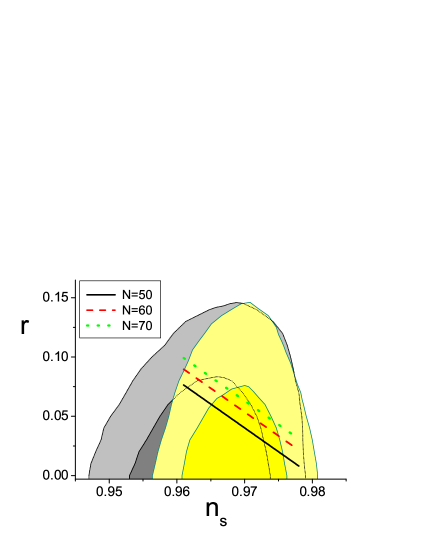
Figure 1: 1$\sigma$ (yellow) and 2$\sigma$ (light yellow) contours for Planck 2015 results ($TT+lowP+lensing+BAO+JLA+H_{0}$) [86], and 1$\sigma$ (grey) and 2$\sigma$ (light grey) contours for Planck 2013 results ($Planck+WP+BAO$) [85] (note that the 1$\sigma$ region of Planck 2013 results is behind the Planck 2015 results, hence we mark its boundary by a dotted curve), on $n_{S}-r$ plane. Additionally, we depict the predictions of our scenario, for the power-law case (3.1), with the e-folding value $N$ being $50$, $60$ and $70$.

Finally, the running of the scalar spectral index is defined as

$$\alpha_{S}\equiv\frac{dn_{S}}{d\ln k}.$$ (3.13)

Hence, since from the definitions of $n_{S}$ and $n_{T}$ one can find [84]

$$\frac{dN}{d\ln k}=\left(1+\frac{d\ln H}{d\ln k}\right)^{-1}\simeq(1+\epsilon_{1}),$$ (3.14)

we can use (3.8), (3.13) and (3.14) in order to express $\alpha_{S}$ as

$$\!\!\!\!\!\!\!\!\!\!\!\!\!\!\!\alpha_{S}=\frac{dn_{S}}{dN}\frac{dN}{d\ln k}\simeq\frac{8(n+1)(3n+1)[(n+1)N+n]}{[2(n+1)N+n]^{3}}.$$ (3.15)

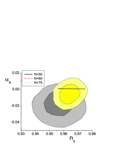
Figure 2: 1$\sigma$ (yellow) and 2$\sigma$ (light yellow) contours for Planck 2015 results ($TT,TE,EE+lowP$) [86], and 1$\sigma$ (grey) and 2$\sigma$ (light grey) contours for Planck 2013 results ($\Lambda CDM+running+tensors$) [85], on $n_{S}-\alpha_{S}$ plane. Additionally, we depict the predictions of our scenario, for the power-law case (3.1), with the e-folding value $N$ being $50$, $60$ and $70$. The various curves are indistinguishable in the resolution scale of the graph.

Thus, eliminating $n$ between (3.8) and (3.15) we obtain $\alpha_{S}$ as a function of $n_{S}$, namely

$$\alpha_{S}\simeq\frac{(n_{S}-1)(n_{S}+3)[(n_{S}-5)N+2]}{(4N-1)^{2}}.$$ (3.16)

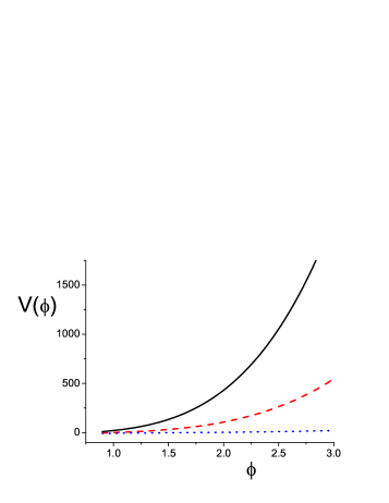
Figure 3: The scalar potential $V(\phi)$ according to expression (3.3), for the power-law case (3.1), for $M=0.1$, $\alpha=1$, $n=2$ (black-solid), for $M=0.1$, $\alpha=0.5$, $n=2$ (red-dashed), and for $M=0.1$, $\alpha=0.1$, $n=2$ (blue-dotted). All quantities are measured in $M_{P}$ units.

In order to present these features more transparently, in Fig. 1 we present the predictions of our scenario with the e-folding value ${N}$ being $50$, $60$ and $70$, on top of the 1$\sigma$ and 2$\sigma$ contours of the Planck 2013 results [85] as well as of the Planck 2015 results [86]. As we observe, the scenario at hand is in very good agreement with observations, with the agreement being better for lower $N$. Additionally, in Fig. 2 we depict the predictions of the scenario at hand for the running spectral index $\alpha_{S}$ with the e-folding value ${N}$ being $50$, $60$ and $70$, on top of the 1$\sigma$ and 2$\sigma$ contours of the Planck 2013 results [85] as well as of the Planck 2015 results [86]. The agreement with observations is very satisfactory.

Finally, in order to provide a picture of the scalar potential, we use expression (3.3) and in Fig. 3 we depict $V(\phi)$ for various values of $M$, $\alpha$ and $n$. In this Figure we have focused on the $\phi$-values in which $\phi_{i}$ according to (3.7) and $\phi_{e}$ according to (3.6) lie.

3.2 Hubble parameter as exponential function

In this subsection we study the case where the Hubble parameter is an exponential function of the scalar field, namely

$$H(\phi)=\beta e^{q\phi},$$ (3.17)

where $\beta$ and $q$ are the model parameters. In this case Eq. (2.13) gives

$$\dot{\phi}\approx-\frac{2q}{3\beta}{M^{2}M_{P}^{2}e^{-q\phi}}\,,$$ (3.18)

and therefore inserting this expression into (2.15) we acquire the potential as

$$\!\!\!\!\!\!\!V(\phi)=27M_{P}^{2}\beta^{2}e^{2q\phi}-18M_{P}^{2}M^{2}\frac{q^{2}}{\beta^{2}e^{2q\phi}}\left(9\beta^{2}e^{2q\phi}+M^{2}\right)\,.$$ (3.19)

The above potential is a sum of exponential potentials, and potentials of these forms are often used in cosmological applications [87, 88, 89, 90, 91, 92, 93, 94].

Furthermore, the slow-roll parameters (2.16),(2.17) become respectively

$$\epsilon_{1}(\phi)\approx\frac{2q^{2}}{3\beta^{2}}M^{2}M_{P}^{2}\,e^{-2q\phi}\,,$$ (3.20)

$$\epsilon_{2}(\phi)\approx\frac{4q^{2}}{3\beta^{2}}M^{2}M_{P}^{2}\,e^{-2q\phi}\,,$$ (3.21)

and we can then impose the condition $\epsilon_{1}(\phi)=1$ in order to calculate the scalar field at the end of inflation as

$$\phi_{e}=\frac{1}{2q}\ln\left(\frac{2M^{2}M_{P}^{2}\,q^{2}}{3\beta^{2}}\right)\,.$$ (3.22)

Additionally, we can use (2.19) and (3.17),(3.18) and extract the value of the scalar field at the beginning of inflation as a function of the e-folding number as

$$\phi_{i}=\frac{1}{2q}\ln\left[\frac{2M^{2}M_{P}^{2}\,q^{2}}{3\beta^{2}}\left(2N+1\right)\right]\,.$$ (3.23)

Concerning the scalar and tensor spectral indices and the tensor-to-scalar ratio, we obtain [77]

$$n_{S}-1 \simeq -2\epsilon_{1}(\phi_{i})-2\epsilon_{2}(\phi_{i})=-\frac{6}{2N+1}\,,$$ (3.24)

$$n_{T} \simeq -2\epsilon_{1}(\phi_{i})=-\frac{2}{2N+1}\,,$$ (3.25)

$$r = -8n_{T}\,,$$ (3.26)

where from the first two of the above expressions we acquire $n_{S}-1=3n_{T}$. Hence, from Eqs.(3.24),(3.25) and (3.26) we can obtain

$$r=\frac{8}{3}-\frac{8}{3}n_{S}$$ (3.27)

and

$$n_{T}=-\frac{1}{3}+\frac{1}{3}n_{S},$$ (3.28)

which prove to be very useful, since they allow us to confront our model predictions straightaway with the data. Note that the parameters $\beta$ and $q$ do not appear in the final parametric expressions, as well as the e-folding number $N$. Finally, the running of the scalar spectral index reads as $\alpha_{S}=\frac{dn_{S}}{dN}\frac{dN}{d\ln k}\simeq\frac{dn_{S}}{dN}\,(1+\epsilon_{1})$, which with the help of (3.20),(3.24) becomes

$$\!\!\!\!\!\!\!\!\!\!\!\!\!\!\!\alpha_{S}\simeq\frac{24(N+1)}{(2N+1)^{3}},$$ (3.29)

and therefore eliminating $N$ using (3.24) we finally acquire

$$\alpha_{S}\simeq\frac{1}{18}(n_{S}-7)(n_{S}-1)^{2}.$$ (3.30)

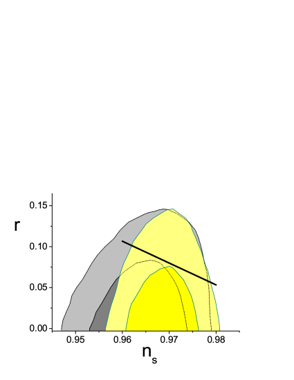
Figure 4: 1$\sigma$ (yellow) and 2$\sigma$ (light yellow) contours for Planck 2015 results ($TT+lowP+lensing+BAO+JLA+H_{0}$) [86], and 1$\sigma$ (grey) and 2$\sigma$ (light grey) contours for Planck 2013 results ($Planck+WP+BAO$) [85] (note that the 1$\sigma$ region of Planck 2013 results is behind the Planck 2015 results, hence we mark its boundary by a dotted curve), on $n_{S}-r$ plane. Additionally, with the black solid line we depict the prediction of our scenario, for the exponential case (3.17), which according to relation (3.27) does not depend on $\beta$, $q$ and $N$.

In order to present these features in a more clear way, in Fig. 4 we illustrate the predictions of our scenario on $n_{S}-r$ plane, on top of the 1$\sigma$ and 2$\sigma$ contours of the Planck 2013 results [85] as well as of the Planck 2015 results [86]. As we mentioned above, according to relation (3.27) the predictions of our scenario do not depend on $\beta$, $q$ and $N$, however they are still in agreement with observations at 2$\sigma$ level. Furthermore, in Fig. 5 we show the predictions of the scenario at hand for the running spectral index $\alpha_{S}$, on top of the 1$\sigma$ and 2$\sigma$ contours of the Planck 2013 results [85] as well as of the Planck 2015 results [86]. According to relation (3.30) the model predictions are independent of $\beta$, $q$ and $N$, however they are in very good agreement with observations.

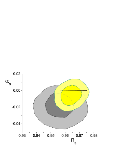
Figure 5: 1$\sigma$ (yellow) and 2$\sigma$ (light yellow) contours for Planck 2015 results ($TT,TE,EE+lowP$) [86], and 1$\sigma$ (grey) and 2$\sigma$ (light grey) contours for Planck 2013 results ($\Lambda CDM+running+tensors$) [85], on $n_{S}-\alpha_{S}$ plane. Additionally, we depict the predictions of our scenario, for the exponential case (3.17), for the e-folding value $N$ being $50$ and $60$. The two curves are indistinguishable in the resolution scale of the graph.

Figure 6: The scalar potential $V(\phi)$ according to expression (3.19), for the exponential case (3.17), for $M=0.1$, $\beta=0.5$, $q=0.5$ (black-solid), for $M=0.1$, $\beta=0.3$, $q=0.5$ (red-dashed), and for $M=0.1$, $\beta=0.5$, $q=0.1$ (blue-dotted). All quantities are measured in $M_{P}$ units.

Lastly, in order to give a picture of the scalar potential, we use expression (3.19) and in Fig. 6 we show $V(\phi)$ for various values of $M$, $\beta$ and $q$. In this Figure we have focused on the $\phi$-values in which $\phi_{i}$ according to (3.23) and $\phi_{e}$ according to (3.22) lie.

3.3 Comparison with minimal-coupling case

In this subsection we briefly compare the effect of the nonminimal derivative coupling with the minimal-coupling case, for completeness (although in this simple case slow-roll conditions are hard to be realized and moreover the unitarity bounds of the theory may be violated [56, 95, 96]).

Let us consider action (2.1) without the nonminimal derivative coupling term. In this case, as it is well known, one obtains the standard Friedmann equations, namely $3M_{P}^{2}{H^{2}}=\frac{{{\dot{\phi}}^{2}}}{2}+V(\phi)$ and $3M_{P}^{2}(\dot{H}+{H^{2}})=-\frac{{{\dot{\phi}}^{2}}}{2}+V(\phi)$, while the scalar-field equation reads $\ddot{\phi}+3H\dot{\phi}+{V^{\prime}}(\phi)=0$. Hence, under the slow-roll conditions,$\frac{{{\dot{\phi}}^{2}}}{2}\ll V(\phi)$ and $|{\ddot{\phi}}|\ll H|{\dot{\phi}}|$, we obtain the following constraints

$$3M_{P}^{2}H^{2}\simeq V(\phi),$$ (3.31)

$${{\dot{\phi}}}\simeq-\frac{{V^{\prime}}(\phi)}{{3H}},$$ (3.32)

which easily lead to ${V^{\prime}}(\phi)\simeq 6M_{P}^{2}HH^{\prime}(\phi)$ and thus to

$$\dot{\phi}\simeq-2M_{P}^{2}H^{\prime}(\phi).$$ (3.33)

Therefore, in this case, substitution into the first Friedmann equations gives the Hamilton-Jacobi equation as

$${H^{\prime}}^{2}(\phi)-3M_{P}^{2}H^{2}(\phi)+\frac{M_{P}^{4}}{2}V(\phi)=0,$$ (3.34)

and thus the potential in terms of the scalar field is expressed as

$$V(\phi)=\frac{6}{M_{P}^{2}}H^{2}(\phi)-\frac{2}{M_{P}^{4}}{H^{\prime}}^{2}(\phi).$$ (3.35)

Finally, the slow-roll parameters read as

$$\epsilon_{1}(\phi)\equiv-\frac{\dot{H}}{H^{2}}\approx 2M_{P}^{2}\left[\frac{H^{\prime}(\phi)}{H(\phi)}\right]^{2}\,,$$ (3.36)

$$\epsilon_{2}(\phi)\equiv\frac{\ddot{H}}{H\dot{H}}-\frac{2\dot{H}}{H^{2}}\approx 4M_{P}^{2}\left\{\left[\frac{H^{\prime}(\phi)}{H(\phi)}\right]^{2}-\frac{H^{\prime\prime}(\phi)}{H(\phi)}\right\}\,,$$ (3.37)

and the e-folding number is still given by (2.19).

Let us now apply the above for the case of the power-law function of (3.1), namely for $H(\phi)=\alpha\phi^{n}$. In this case Eq. (3.33) becomes

$$\dot{\phi}\approx-2M_{P}^{2}\,n\alpha{\phi^{n-1}}\,,$$ (3.38)

while (3.35) reads

$$\!\!\!\!\!\!\!V(\phi)=\frac{6}{M_{P}^{2}}\alpha^{2}\phi^{2n}-\frac{2}{M_{P}^{4}}\alpha^{2}{n^{2}}\phi^{2(n-1)}.$$ (3.39)

Additionally, the slow-roll parameters (3.36),(3.37) become

$$\epsilon_{1}(\phi)\approx 2M_{P}^{2}\frac{n^{2}}{\phi^{2}},$$ (3.40)

$$\epsilon_{2}(\phi)\approx 4M_{P}^{2}\frac{n}{\phi^{2}},$$ (3.41)

while the scalar field at the end of inflation, corresponding to $\epsilon_{1}(\phi_{e})=1$, is given by

$$\phi_{e}=\sqrt{2}nM_{P}.$$ (3.42)

Additionally, using (2.19) and (3.33), the scalar field at the beginning of inflation becomes

$${\phi_{i}}=M_{P}\sqrt{2n(n+2N)}.$$ (3.43)

Hence, inserting these in the expressions of the inflationary observables we finally obtain

$${n_{S}}-1\simeq-2\epsilon_{1}(\phi_{i})-2\epsilon_{2}(\phi_{i})=-\frac{2(n+2)}{n+2N},$$ (3.44)

$$n_{T}\simeq-2\epsilon_{1}(\phi_{i})=-\frac{2n}{n+2N},$$ (3.45)

$$r=-8n_{T}\,.$$ (3.46)

Similarly, for the case of the exponential function of (3.17), namely for $H(\phi)=\beta e^{q\phi}$, we obtain

$$\dot{\phi}\approx-2M_{P}^{2}\,\beta qe^{q\phi}\,,$$ (3.47)

while (3.35) reads

$$\!\!\!\!\!\!\!V(\phi)=\frac{6}{M_{P}^{2}}\beta^{2}e^{2q\phi}-\frac{2}{M_{P}^{4}}\beta^{2}q^{2}e^{2q\phi}.$$ (3.48)

However, the slow-roll parameters (3.36),(3.37) become

$$\epsilon_{1}(\phi)\approx 2q^{2}M_{P}^{2},$$ (3.50)

$$\epsilon_{2}(\phi)\approx 0.$$

Thus, we can immediately see that the exponential form in the case of minimal coupling cannot describe inflation successfully, since $\epsilon_{1}=const.$.

One can see that the above relations, which have been extracted in the case of minimal-coupling, are different from the expressions of the previous subsections which were extracted in the case of nonminimal derivative coupling. In particular, in the power-law case relations (3.44)-(3.46) are different from (3.8)-(3.10), while in the exponential case a successful realization of inflation is not possible. Furthermore, relations (3.44)-(3.46) cannot fit the observational data. Actually, these disadvantages were one of the reasons that inflation with nonminimal derivative coupling was introduced in [56]. Hence, we conclude that the nonminimal derivative coupling plays an important role, both quantitatively (one has an additional parameter to fit the data) and qualitatively (the unitarity issue is solved).

4 Conclusion

In this work we have investigated inflation with nonminimal derivative coupling through the Hamilton-Jacobi formalism. In the majority of inflationary models one can perform the conformal transformation to the Einstein frame, where the calculation of inflationary observables is straightforward, however in inflation with nonminimal derivative such a transformation is absent and thus a detailed and lengthy perturbation analysis is needed in order to provide inflationary observables that could be compared with the data. Hence, in such a case the Hamilton-Jacobi analysis proves to be a very convenient method to extract the scenario prediction for various observables.

In the Hamilton-Jacobi formalism one rewrites the cosmological equations by considering the scalar field to be the time variable, which is always possible during the slow-roll era, where the scalar varies monotonically (the extension to the post-inflationary, oscillatory epoch is straightforward by matching together separate monotonic epochs). We have performed such an analysis in inflation with nonminimal derivative coupling, and we have applied it to two specific models for the Hubble function, namely the power-law and the exponential cases. For each model we have calculated various observables such as the tensor-to-scalar ratio, and the spectral index and its running, and we have compared them with the Planck data.

For the case of power-law form we have shown that the tensor-to-scalar ratio and the tensor spectral index have a linear dependence on the scalar spectral index, with its properties depending on the model parameters and the e-folding number, and confrontation with 2013 and 2015 Planck results shows a very good agreement. Additionally, the predictions for the running spectral index are also in very good agreement with the data. Finally, for transparency we have provided the corresponding profile of the scalar potential.

For the case of exponential form the tensor-to-scalar ratio and the tensor spectral index have a linear dependence on the scalar spectral index too, however not depending on the model parameters or the e-folding number. Nevertheless, the predictions are in good agreement with observational data. The behavior of the running spectral index is more complicated, but still in very good agreement with the Planck results.

Finally, comparing our results with the case of minimal coupling, we saw that the nonminimal derivative coupling can fit the data more efficiently, as well as solve the unitarity problems of the minimal theory.

The above features reveal that the Hamilton-Jacobi formalism can be very efficient in analyzing inflationary models which do not allow for a conformal transformation to the Einstein frame. And indeed, its application shows that inflation with nonminimal derivative coupling is in agreement with observations and thus it can be a good candidate for the description of Nature.

References

- [1] D. Kazanas, Dynamics of the Universe and Spontaneous Symmetry Breaking, Astrophys. J. 241, L59 (1980).
- [2] A. H. Guth, The Inflationary Universe: A Possible Solution to the Horizon and Flatness Problems, Phys. Rev. D 23, 347 (1981).
- [3] A. A. Starobinsky, A New Type of Isotropic Cosmological Models Without Singularity, Phys. Lett. B 91, 99 (1980).
- [4] K. Sato, First Order Phase Transition of a Vacuum and Expansion of the Universe, Mon. Not. Roy. Astron. Soc. 195, 467 (1981).
- [5] A. A. Starobinsky, Dynamics of Phase Transition in the New Inflationary Universe Scenario and Generation of Perturbations, Phys. Lett. B 117, 175 (1982).
- [6] A. D. Linde, A New Inflationary Universe Scenario: A Possible Solution of the Horizon, Flatness, Homogeneity, Isotropy and Primordial Monopole Problems, Phys. Lett. B 108, 389 (1982).
- [7] A. R. Liddle, An Introduction to cosmological inflation, [arXiv:astro-ph/9901124].
- [8] D. Langlois, Inflation, quantum fluctuations and cosmological perturbations, [arXiv:hep-th/0405053].
- [9] D. H. Lyth and A. Riotto, Particle physics models of inflation and the cosmological density perturbation, Phys. Rept. 314, 1 (1999) [arXiv:hep-th/9807278].
- [10] A. H. Guth, Inflation and eternal inflation, Phys. Rept. 333, 555 (2000) [arXiv:astro-ph/0002156].
- [11] J. E. Lidsey, A. R. Liddle, E. W. Kolb, E. J. Copeland, T. Barreiro and M. Abney, Reconstructing the inflation potential : An overview, Rev. Mod. Phys. 69, 373 (1997) [arXiv:astro-ph/9508078].
- [12] B. A. Bassett, S. Tsujikawa and D. Wands, Inflation dynamics and reheating, Rev. Mod. Phys. 78, 537 (2006) [arXiv:astro-ph/0507632].
- [13] L. P. Grishchuk, Amplification of gravitational waves in an istropic universe, Sov. Phys. JETP 40, 409 (1975) [Zh. Eksp. Teor. Fiz. 67, 825 (1974)].
- [14] A. A. Starobinsky, Spectrum of relict gravitational radiation and the early state of the universe, JETP Lett. 30, 682 (1979) [Pisma Zh. Eksp. Teor. Fiz. 30, 719 (1979)].
- [15] B. Allen, The Stochastic Gravity Wave Background in Inflationary Universe Models, Phys. Rev. D 37, 2078 (1988).
- [16] V. Sahni, The Energy Density of Relic Gravity Waves From Inflation, Phys. Rev. D 42, 453 (1990).
- [17] T. Souradeep and V. Sahni, Density perturbations, gravity waves and the cosmic microwave background, Mod. Phys. Lett. A 7, 3541 (1992) [arXiv:hep-ph/9208217].
- [18] M. Giovannini, Spikes in the relic graviton background from quintessential inflation, Class. Quant. Grav. 16, 2905 (1999) [arXiv:hep-ph/9903263].
- [19] M. Sami and V. Sahni, Quintessential inflation on the brane and the relic gravity wave background, Phys. Rev. D 70, 083513 (2004) [arXiv:hep-th/0402086].
- [20] M. Wali Hossain, R. Myrzakulov, M. Sami and E. N. Saridakis, Unification of inflation and dark energy á la quintessential inflation, Int. J. Mod. Phys. D 24, no. 05, 1530014 (2015) [arXiv:1410.6100].
- [21] C. Q. Geng, M. W. Hossain, R. Myrzakulov, M. Sami and E. N. Saridakis, Quintessential inflation with canonical and noncanonical scalar fields and Planck 2015 results, Phys. Rev. D 92, no. 2, 023522 (2015) [arXiv:1502.03597].
- [22] M. W. Hossain, R. Myrzakulov, M. Sami and E. N. Saridakis, Class of quintessential inflation models with parameter space consistent with BICEP2, Phys. Rev. D 89, no. 12, 123513 (2014) [arXiv:1404.1445].
- [23] Y. F. Cai, J. O. Gong, S. Pi, E. N. Saridakis and S. Y. Wu, On the possibility of blue tensor spectrum within single field inflation, Nucl. Phys. B 900, 517 (2015) [arXiv:1412.7241].
- [24] S. Nojiri and S. D. Odintsov, Modified gravity with negative and positive powers of the curvature: Unification of the inflation and of the cosmic acceleration, Phys. Rev. D 68, 123512 (2003) [arXiv:hep-th/0307288].
- [25] S. Nojiri and S. D. Odintsov, Unifying phantom inflation with late-time acceleration: Scalar phantom-non-phantom transition model and generalized holographic dark energy, Gen. Rel. Grav. 38, 1285 (2006) [arXiv:hep-th/0506212].
- [26] S. Capozziello, S. Nojiri and S. D. Odintsov, Unified phantom cosmology: Inflation, dark energy and dark matter under the same standard, Phys. Lett. B 632, 597 (2006) [arXiv:hep-th/0507182].
- [27] S. Capozziello and M. De Laurentis, Extended Theories of Gravity, Phys. Rept. 509, 167 (2011) [arXiv:1108.6266].
- [28] A. D. Linde, Chaotic Inflation, Phys. Lett. B 129, 177 (1983).
- [29] A. Albrecht and P. J. Steinhardt, Cosmology for Grand Unified Theories with Radiatively Induced Symmetry Breaking, Phys. Rev. Lett. 48, 1220 (1982).
- [30] K. Freese, J. A. Frieman and A. V. Olinto, Natural inflation with pseudo - Nambu-Goldstone bosons, Phys. Rev. Lett. 65, 3233 (1990).
- [31] Y. S. Piao and Y. Z. Zhang, Phantom inflation and primordial perturbation spectrum, Phys. Rev. D 70, 063513 (2004) [arXiv:astro-ph/0401231].
- [32] J. E. Lidsey, Triality between inflation, cyclic and phantom cosmologies, Phys. Rev. D 70, 041302 (2004) [arXiv:gr-qc/0405055].
- [33] E. Elizalde, S. Nojiri, S. D. Odintsov, D. Saez-Gomez and V. Faraoni, Reconstructing the universe history, from inflation to acceleration, with phantom and canonical scalar fields, Phys. Rev. D 77, 106005 (2008) [arXiv:0803.1311].
- [34] C. J. Feng, X. Z. Li and E. N. Saridakis, Preventing eternality in phantom inflation, Phys. Rev. D 82, 023526 (2010) [arXiv:1004.1874].
- [35] M. Fairbairn and M. H. G. Tytgat, Inflation from a tachyon fluid?, Phys. Lett. B 546, 1 (2002) [arXiv:hep-th/0204070].
- [36] A. Feinstein, Power law inflation from the rolling tachyon, Phys. Rev. D 66, 063511 (2002) [arXiv:hep-th/0204140].
- [37] A. Aghamohammadi, A. Mohammadi, T. Golanbari and K. Saaidi, Hamilton-Jacobi formalism for tachyon inflation, Phys. Rev. D 90, no. 8, 084028 (2014) [arXiv:1502.07578].
- [38] C. Armendariz-Picon, T. Damour and V. F. Mukhanov, k - inflation, Phys. Lett. B 458, 209 (1999) [arXiv:hep-th/9904075].
- [39] H. Sheikhahmadi, S. Ghorbani and K. Saaidi, Non-local scalar fields inflationary mechanism in light of Planck , Astrophys. Space Sci. 357, no. 2, 115 (2015) [arXiv:1502.05166].
- [40] N. Arkani-Hamed, P. Creminelli, S. Mukohyama and M. Zaldarriaga, Ghost inflation, JCAP 0404, 001 (2004) [arXiv:hep-th/0312100].
- [41] R. Fakir and W. G. Unruh, Improvement on cosmological chaotic inflation through nonminimal coupling, Phys. Rev. D 41, 1783 (1990).
- [42] V. Sahni and S. Habib, Does inflationary particle production suggest Omega(m) less than 1?, Phys. Rev. Lett. 81, 1766 (1998) [arXiv:hep-ph/9808204].
- [43] J. P. Uzan, Cosmological scaling solutions of nonminimally coupled scalar fields, Phys. Rev. D 59, 123510 (1999) [arXiv:gr-qc/9903004].
- [44] V. Faraoni, Inflation and quintessence with nonminimal coupling, Phys. Rev. D 62, 023504 (2000) [arXiv:gr-qc/0002091].
- [45] S. Tsujikawa, Power law inflation with a nonminimally coupled scalar field, Phys. Rev. D 62, 043512 (2000) [arXiv:hep-ph/0004088].
- [46] Y. S. Piao, Q. G. Huang, X. m. Zhang and Y. Z. Zhang, Nonminimally coupled tachyon and inflation, Phys. Lett. B 570, 1 (2003) [arXiv:hep-ph/0212219].
- [47] S. Tsujikawa and B. Gumjudpai, Density perturbations in generalized Einstein scenarios and constraints on nonminimal couplings from the Cosmic Microwave Background, Phys. Rev. D 69, 123523 (2004) [arXiv:astro-ph/0402185].
- [48] D. I. Kaiser and E. I. Sfakianakis, Multifield Inflation after Planck: The Case for Nonminimal Couplings, Phys. Rev. Lett. 112, no. 1, 011302 (2014) [arXiv:1304.0363].
- [49] L. Amendola, Cosmology with nonminimal derivative couplings, Phys. Lett. B 301, 175 (1993) [arXiv:gr-qc/9302010].
- [50] S. Capozziello and G. Lambiase, Nonminimal derivative coupling and the recovering of cosmological constant, Gen. Rel. Grav. 31, 1005 (1999) [arXiv:gr-qc/9901051].
- [51] S. Capozziello, G. Lambiase and H. J. Schmidt, Nonminimal derivative couplings and inflation in generalized theories of gravity, Annalen Phys. 9, 39 (2000) [arXiv:gr-qc/9906051].
- [52] S. F. Daniel and R. R. Caldwell, Consequences of a cosmic scalar with kinetic coupling to curvature, Class. Quant. Grav. 24, 5573 (2007) [arXiv:0709.0009].
- [53] A. B. Balakin, H. Dehnen and A. E. Zayats, Effective metrics in the non-minimal Einstein-Yang-Mills-Higgs theory, Annals Phys. 323, 2183 (2008) [arXiv:0804.2196].
- [54] E. N. Saridakis and S. V. Sushkov, Quintessence and phantom cosmology with non-minimal derivative coupling, Phys. Rev. D 81, 083510 (2010) [arXiv:1002.3478].
- [55] C. Gao, When scalar field is kinetically coupled to the Einstein tensor, JCAP 1006, 023 (2010) [arXiv:1002.4035].
- [56] C. Germani and A. Kehagias, New Model of Inflation with Non-minimal Derivative Coupling of Standard Model Higgs Boson to Gravity, Phys. Rev. Lett. 105, 011302 (2010) [arXiv:1003.2635].
- [57] L. N. Granda, Inflation driven by scalar field with non-minimal kinetic coupling with Higgs and quadratic potentials, JCAP 1104, 016 (2011) [arXiv:1104.2253].
- [58] V. K. Shchigolev and M. P. Rotova, A tachyon cosmological model with non-minimal derivative coupling to gravity, Gravit. Cosmol. 18, no. 1, 88 (2012) [arXiv:1105.4536].
- [59] S. Tsujikawa, Observational tests of inflation with a field derivative coupling to gravity, Phys. Rev. D 85, 083518 (2012) [arXiv:1201.5926].
- [60] H. M. Sadjadi and P. Goodarzi, Reheating in nonminimal derivative coupling model, JCAP 1302, 038 (2013) [arXiv:1203.1580].
- [61] H. M. Sadjadi and P. Goodarzi, Reheating temperature in non-minimal derivative coupling model, JCAP 1307, 039 (2013) [arXiv:1302.1177].
- [62] G. Koutsoumbas, K. Ntrekis and E. Papantonopoulos, Gravitational Particle Production in Gravity Theories with Non-minimal Derivative Couplings, JCAP 1308, 027 (2013) [arXiv:1305.5741].
- [63] K. Feng, T. Qiu and Y. S. Piao, Curvaton with nonminimal derivative coupling to gravity, Phys. Lett. B 729, 99 (2014) [arXiv:1307.7864].
- [64] H. M. Sadjadi and P. Goodarzi, Oscillatory inflation in non-minimal derivative coupling model, Phys. Lett. B 732, 278 (2014) [arXiv:1309.2932].
- [65] J. B. Dent, S. Dutta, E. N. Saridakis and J. Q. Xia, Cosmology with non-minimal derivative couplings:perturbation analysis and observational constraints, JCAP 1311, 058 (2013) [arXiv:1309.4746].
- [66] M. A. Skugoreva, A. V. Toporensky and S. Y. Vernov, Global stability analysis for cosmological models with nonminimally coupled scalar fields, Phys. Rev. D 90, no. 6, 064044 (2014) [arXiv:1404.6226].
- [67] N. Yang, Q. Gao and Y. Gong, Inflationary models with non-minimally derivative coupling, [arXiv:1504.05839].
- [68] G. Koutsoumbas, K. Ntrekis, E. Papantonopoulos and M. Tsoukalas, Gravitational Collapse in Horndeski Theory, [arXiv:1512.05934].
- [69] G. W. Horndeski, Second-order scalar-tensor field equations in a four-dimensional space, Int. J. Theor. Phys. 10 (1974) 363.
- [70] A. Nicolis, R. Rattazzi and E. Trincherini, The Galileon as a local modification of gravity, Phys. Rev. D 79, 064036 (2009) [arXiv:0811.2197].
- [71] C. Deffayet, G. Esposito-Farese and A. Vikman, Covariant Galileon, Phys. Rev. D 79, 084003 (2009) [arXiv:0901.1314].
- [72] A. Padilla, P. M. Saffin and S. Y. Zhou, Bi-galileon theory II: Phenomenology, JHEP 1101, 099 (2011) [arXiv:1008.3312].
- [73] E. N. Saridakis and M. Tsoukalas, Cosmology in new gravitational scalar-tensor theories, Phys. Rev. D 93, no. 12, 124032 (2016) [arXiv:1601.06734].
- [74] E. N. Saridakis and M. Tsoukalas, Bi-scalar modified gravity and cosmology with conformal invariance, JCAP 1604, no. 04, 017 (2016) [arXiv:1602.06890].
- [75] D. S. Salopek and J. R. Bond, Nonlinear evolution of long wavelength metric fluctuations in inflationary models, Phys. Rev. D 42, 3936 (1990).
- [76] A. R. Liddle and D. H. Lyth, Cosmological inflation and large scale structure, Cambridge, UK: Univ. Pr. (2000) 400 p.
- [77] J. Martin, C. Ringeval and V. Vennin, Encyclopaedia Inflationaris, Phys. Dark Univ. 5-6, 75 (2014) [arXiv:1303.3787].
- [78] P. J. E. Peebles and B. Ratra, Cosmology with a Time Variable Cosmological Constant, Astrophys. J. 325, L17 (1988).
- [79] L. R. W. Abramo and F. Finelli, Cosmological dynamics of the tachyon with an inverse power-law potential, Phys. Lett. B 575, 165 (2003), [arXiv:astro-ph/0307208].
- [80] J. M. Aguirregabiria and R. Lazkoz, Tracking solutions in tachyon cosmology, Phys. Rev. D 69, 123502 (2004), [arXiv:hep-th/0402190].
- [81] E. J. Copeland, M. R. Garousi, M. Sami and S. Tsujikawa, What is needed of a tachyon if it is to be the dark energy?, Phys. Rev. D 71, 043003 (2005), [arXiv:hep-th/0411192].
- [82] E. N. Saridakis, Phantom evolution in power-law potentials, Nucl. Phys. B 819, 116 (2009), [arXiv:0902.3978].
- [83] M. A. Skugoreva, S. V. Sushkov and A. V. Toporensky, Cosmology with nonminimal kinetic coupling and a power-law potential, Phys. Rev. D 88, 083539 (2013), [arXiv:1306.5090].
- [84] D. Baumann, TASI Lectures on Inflation [arXiv:0907.5424].
- [85] P. A. R. Ade et al. [Planck Collaboration], Planck 2013 results. XXII. Constraints on inflation, Astron. Astrophys. 571, A22 (2014) [arXiv:1303.5082].
- [86] P. A. R. Ade et al. [Planck Collaboration], Planck 2015 results. XIII. Cosmological parameters, [arXiv:1502.01589].
- [87] J. J. Halliwell, Scalar Fields in Cosmology with an Exponential Potential, Phys. Lett. B 185 (1987) 341.
- [88] J. M. Aguirregabiria, A. Feinstein and J. Ibanez, Exponential potential scalar field universes. 1. The Bianchi I models, Phys. Rev. D 48, 4662 (1993), [arXiv:gr-qc/9309013].
- [89] J. M. Aguirregabiria, A. Feinstein and J. Ibanez, Exponential potential scalar field universes. 2. The Inhomogeneous models, Phys. Rev. D 48 (1993) 4669, [arXiv:gr-qc/9309014].
- [90] A. A. Coley, J. Ibanez and R. J. van den Hoogen, Homogeneous scalar field cosmologies with an exponential potential, J. Math. Phys. 38 (1997) 5256.
- [91] E. J. Copeland, A. R. Liddle and D. Wands, Exponential potentials and cosmological scaling solutions, Phys. Rev. D 57, 4686 (1998). [arXiv:gr-qc/9711068].
- [92] T. Barreiro, E. J. Copeland and N. J. Nunes, Quintessence arising from exponential potentials, Phys. Rev. D 61 (2000) 127301, [arXiv:astro-ph/9910214].
- [93] I. P. C. Heard and D. Wands, Cosmology with positive and negative exponential potentials, Class. Quant. Grav. 19 (2002) 5435, [arXiv:gr-qc/0206085].
- [94] C. Rubano, P. Scudellaro, E. Piedipalumbo, S. Capozziello and M. Capone, Exponential potentials for tracker fields, Phys. Rev. D 69 (2004) 103510, [arXiv:astro-ph/0311537].
- [95] C. P. Burgess, H. M. Lee and M. Trott, Power-counting and the Validity of the Classical Approximation During Inflation, JHEP 0909, 103 (2009) [arXiv:0902.4465].
- [96] R. N. Lerner and J. McDonald, Higgs Inflation and Naturalness, JCAP 1004, 015 (2010) [arXiv:0912.5463].