Thermo-magnetic effects in quark matter: Nambu–Jona-Lasinio model constrained by lattice QCD

Abstract

The phenomenon of inverse magnetic catalysis of chiral symmetry in QCD predicted by lattice simulations can be reproduced within the Nambu–Jona-Lasinio model if the coupling $G$ of the model decreases with the strength $B$ of the magnetic field and temperature $T$. The thermo-magnetic dependence of $G(B,T)$ is obtained by fitting recent lattice QCD predictions for the chiral transition order parameter. Different thermodynamic quantities of magnetized quark matter evaluated with $G(B,T)$ are compared with the ones obtained at constant coupling, $G$. The model with $G(B,T)$ predicts a more dramatic chiral transition as the field intensity increases. In addition, the pressure and magnetization always increase with $B$ for a given temperature. Being parametrized by four magnetic field dependent coefficients and having a rather simple exponential thermal dependence our accurate ansatz for the coupling constant can be easily implemented to improve typical model applications to magnetized quark matter.

The fact that strong magnetic fields may be generated in peripheral heavy-ion collisions heavyion1 ; heavyion2 and may also be present in magnetars magnetars has motivated many recent investigations regarding the effects of a magnetic field in defining the boundaries of the quantum chromodynamics (QCD) phase diagram — for recent reviews, see Refs. Miransky:2015ava ; revandersen . In both situations, the magnitude of the magnetic fields is huge and may reach respectively $10^{19}\,{\rm G}$ and $10^{18}\,{\rm G}$. In heavy ion collisions, the presence of a strong magnetic field most certainly plays a role, despite the fact that the field intensity might decrease very rapidly, lasting for about $1-2\leavevmode\nobreak\ {\rm fm}/{\rm c}$ only heavyion1 ; heavyion2 . The possibility that this short time interval may tuchin or may not mclerran be affected by conductivity remains under dispute. Very interesting effects are also expected in neutron stars with a possible quark core, as the magnetic field penetrates into the quark core in the form of quark vortices due to the presence of Meissner currents david1 ; david2 . At zero temperature, the great majority of effective models for QCD are in agreement with respect to the occurrence of the phenomenon of magnetic catalysis (MC), which refers to the increase of the chiral order parameter represented by the (light) quark condensates with the strenght $B$ of the magnetic field. On the other hand, at finite temperature such models fail to predict the inverse magnetic catalysis (IMC), an effect discovered by lattice QCD (LQCD) simulations lattice ; fodor , in that the pseudo-critical temperature $T_{pc}$ for chiral symmetry partial restoration decreases as $B$ increases. We remark that LQCD simulations as well as most models predict that the crossover transition observed at $B=0$ and vanishing chemical potential survives the presence of a background magnetic field, at least for realistic field intensities. The failure of model calculations in predicting IMC at high temperatures has motivated a large body of work attempting to clarify the reasons for the observed discrepancies Miransky:2015ava ; revandersen ; fragaMIT ; prl ; kojo ; endrodi ; leticiaLN ; EPNJL1 ; EPNJL2 ; EPNJL3 ; debora ; bruno ; bonati ; ayala1 ; ferreira1 ; ayala2 ; ayala3 ; ferrer1 ; cao1 ; sadooghi1 ; andersen2 ; kanazawa ; ayala4 ; endrodi2 ; huang1 ; feng1 ; braum1 ; Pawlowski1 ; ayala5 ; endrodi3 ; debora2 ; noronha1 ; marcus1 ; debora1 ; debora3 ; ayala6 ; Cao2 ; Yoshiike ; Hattori1 ; feng2 ; cao3 ; fengli1 ; raya . Intuitively, it is natural to attribute the failure to the fact that most effective models lack gluonic degrees of freedom and so are unable to account for the back reaction of sea quarks to the external magnetic field. This implies, in particular, the absence of asymptotic freedom, a key feature of QCD that plays an important role in processes involving high temperatures and large baryon densities, and, of course, large magnetic fields. Since long ago, such effects have been mimicked in effective models by making the coupling strength to decrease with the temperature and/or density according to some ansatz bernard ; marcus . More recently, this very same strategy was adopted in the case of hot magnetized quark matter. In particular, in Ref. PRCfarias2014 , the IMC phenomenon found by lattice simulations was explained within the two-flavor Nambu–Jona-Lasinio model (NJL) when the coupling constant, $G$, is forced to decrease with both the magnetic field strength $B$ and the temperature $T$, simulating effects not captured with the conventional NJL model. A similar procedure was used with a $SU(3)$ Polyakov-NJL (PNJL) model, but with $G$ depending only on the magnetic field prdferreira ; this leads, however, to a non monotonic decrease of $T_{pc}$ at high field values. In a very recent work ayala7 , an explicit calculation of the one-loop correction to the quark-gluon vertex has shown that competing effects between quark and gluon color charges make the effective quark-gluon coupling to decrease as the strength of the magnetic field increases at finite temperatures. This certainly lends strong support to the idea PRCfarias2014 that the IMC is due to the decrease of the effective coupling between quarks and gluons in the presence of magnetic fields at high temperatures.

In the present paper we investigate the implications of using a $B-$ and $T-$modified NJL coupling for thermodynamic quantities of magnetized quark matter. We are particularly interested in the qualitative changes that a $G(B,T)$ causes in quantities very sensitive to the chiral transition, such as the speed of sound, thermal susceptibility and specific heat. This is an important open question since the interaction that is implied by a $G(B,T)$ gives rise to a new phenomenology that has not been fully explored in the literature. The investigation of the correlation between a $T$ and $B$ dependence of the NJL coupling $G$ used to describe IMC with other physical quantities is important to get further insight into the role played by effects not captured by the normal NJL. As we shall show, the very same $G(B,T)$ required to fit the lattice result for $T_{pc}$, gives results for the pressure, entropy and energy density that are in qualitative agreement with corresponding lattice results, while a $B-$ and $T-$independent coupling gives qualitatively different results for those quantities. This seems to be a clear indication that the $B$ and $T$ dependence in $G$ needed to describe $T_{pc}$ is neither fortuitous nor valid for a single physical quantity only; it seems to capture correctly the physics left out in the conventional NJL model. Instead of the parametrization used in Ref. PRCfarias2014 , based on qualitative arguments referring to asymptotic freedom, in the present paper we base the parametrization of $G$ on a precise fit of recent LQCD calculations. In doing so, one avoids any particular interpretation on the effects behind fitting formulas used for the $B$ and $T$ dependence of $G$, as any interpolation formula of the lattice data points leads to qualitatively similar results for the thermodynamical quantities. We fit LQCD results for the magnetized quark condensates with a particularly simple Fermi-type distribution formula for $G(B,T)$, parametrized by four $B$-dependent coefficients. As we shall demonstrate, one of the main physical implications of using such thermo magnetic effects in the coupling constant is that the signatures associated with the chiral transition in thermodynamic quantities become more markedly defined as the field strength increases. Also, our results for the pressure and magnetization are in line with LQCD predictions, which find that at a fixed temperature, these quantities always increase with $B$. This behavior, especially close to the transition region, is not observed with the NJL model with a $B$ and $T$ independent coupling $G$.

In the next section we review the results for the magnetized NJL pressure within the mean field approximation (MFA). In Sec. III we extract $G(B,T)$ from an accurate fit of LQCD results. Numerical results for different thermodynamical quantities are presented in Sec. IV. Our conclusions and final remarks are presented in Sec. V.

1 Magnetized NJL Pressure

Here we consider the isospin-symmetric two flavor version of the NJL model njl , defined by the Lagrangian density

$$\mathcal{L}_{\rm NJL} = -\frac{1}{4}F^{\mu\nu}F_{\mu\nu}+{\bar{\psi}}\left({\not{D}}-m\right)\psi$$ (1)

$$+ G\left[(\bar{\psi}\psi)^{2}+(\bar{\psi}i\gamma_{5}{\bf\tau}\psi)^{2}\right],$$

where the field $\psi$ represents a flavor iso-doublet of $u$ and $d$ quark flavors and $N_{c}$-plet of quark fields, ${\bf\tau}$ are the isospin Pauli matrices, $D^{\mu}=(i\partial^{\mu}-QA^{\mu})$ the covariant derivative, Q=diag($q_{u}$= $2e/3$, $q_{d}$=-$e/3$) the charge matrix and $A^{\mu}$, $F^{\mu\nu}=\partial^{\mu}A^{\nu}-\partial^{\nu}A^{\mu}$ are respectively the electromagnetic gauge and tensor fields. Since the model is non-renormalizable, we need to specify a regularization scheme. In this work we use a noncovariant cutoff regularization parametrized by $\Lambda$, within the magnetic field independent regularization scheme (MFIR). The MFIR scheme, originally formulated in terms of the proper-time regularization method klimenko , was recently reformulated nosso1 using dimensional regularization by performing a sum over all Landau levels in the vacuum term. In this way, one is able to isolate the divergencies into a term that has the form of the zero magnetic field vacuum energy and thereby can be renormalized in standard fashion. The MFIR was recently employed in the problems of magnetized color superconducting cold matter norberto ; PRDdyana , where its advantages, such as the avoidance of unphysical oscillations, are fully discussed. Other interesting application of MFIR scheme can be found in mfirmpi0 ; mfirplb , where the properties of magnetized neutral mesons were studied. Within this regularization scheme, the cutoff $\Lambda$, the coupling $G$ and the current quark mass $m$ represent free parameters which are fixed klevansky ; buballa by fitting the vacuum values of the pion mass $m_{\pi}$, pion decay constant $f_{\pi}$ and quark condensate $\langle{\bar{\psi}}_{f}\psi_{f}\rangle$.

In the MFA, the NJL pressure in the presence of a magnetic field can be expressed as a sum of quasi-particle and condensate contributions nosso1 ; prdmarcus :

$$P=\frac{B^{2}}{2}+P_{u}+P_{d}-\frac{(M-m)^{2}}{4G},$$ (2)

where $B^{2}/2$ comes from the first term in Eq. (1), and each of the remaining terms can be written as a sum of three terms ($f=u,d$):

$$P_{f} = P_{f}^{vac}+P_{f}^{mag}+P_{f}^{Tmag},$$ (3)

$$\langle{\bar{\psi}}_{f}\psi_{f}\rangle = \langle{\bar{\psi}}_{f}\psi_{f}\rangle^{vac}+\langle{\bar{\psi}}_{f}\psi_{f}\rangle^{mag}+\langle{\bar{\psi}}_{f}\psi_{f}\rangle^{Tmag},$$ (4)

with the quasi-particle terms given by

$$P^{vac}_{f} = \frac{N_{c}M^{4}}{8\pi^{2}}\left[\frac{\epsilon_{\Lambda}\Lambda^{3}}{M^{4}}\left(1+\frac{\epsilon^{2}_{\Lambda}}{\Lambda^{2}}\right)-\ln\left(\frac{\Lambda+\epsilon_{\Lambda}}{M}\right)\right],$$ (5)

$$P^{mag}_{f} = \frac{N_{c}(|q_{f}|B)^{2}}{2\pi^{2}}\biggl{[}\frac{x^{2}_{f}}{4}-\frac{x_{f}}{2}(x_{f}-1)\ln x_{f}$$ (6)

$$+\,\zeta^{\prime}(-1,x_{f})\biggr{]},$$

$$P^{Tmag}_{f} = T\sum_{k=0}^{\infty}\alpha_{k}\frac{|q_{f}|BN_{c}}{2\pi^{2}}$$ (7)

$$\times \int_{-\infty}^{+\infty}dp\,\ln\left\{1+\exp[-(E_{f}/T)]\right\},$$

The quark condensates are given by

$$\langle{\bar{\psi}}_{f}\psi_{f}\rangle^{vac} = -\frac{MN_{c}}{2\pi^{2}}\left[\Lambda\,\epsilon_{\Lambda}-{M^{2}}\ln\left(\frac{\Lambda+\epsilon_{\Lambda}}{{M}}\right)\right],$$ (8)

$$\langle{\bar{\psi}}_{f}\psi_{f}\rangle^{mag} = -\frac{M|q_{f}|BN_{c}}{2\pi^{2}}\biggl{[}\ln\Gamma(x_{f})-\frac{1}{2}\ln(2\pi)$$ (9)

$$+\,x_{f}-\frac{1}{2}\left(2x_{f}-1\right)\ln(x_{f})\biggr{]},$$

$$\langle{\bar{\psi}}_{f}\psi_{f}\rangle^{Tmag} = \sum_{k=0}^{\infty}\alpha_{k}\frac{M|q_{f}|BN_{c}}{2\pi^{2}}\int_{-\infty}^{+\infty}dp\;\frac{n(E_{f})}{E_{f}},$$ (10)

where $\Gamma(x_{f})$ is usual gamma function, and the other quantities appearing in these equations are given by

$$\epsilon_{\Lambda} = \left(\Lambda^{2}+M^{2}\right)^{1/2},$$ (11)

$$E_{f} = \left(p^{2}+M^{2}+2|q_{f}|Bk\right)^{1/2},$$ (12)

$$x_{f} = \frac{M^{2}}{2|q_{f}|B},$$ (13)

$$n(E_{f}) = \frac{1}{1+\exp(E_{f}/T)},$$ (14)

$$\zeta^{\prime}(-1,x_{f}) = \frac{d\zeta(z,x_{f})}{dz}\bigg{|}_{z=-1},$$ (15)

where $\zeta(z,x_{f})$ is the Riemann-Hurwitz zeta function. To take further derivatives of this function, as well as for numerical purposes, it is useful to use the following representation BB

$$\zeta^{\prime}(-1,x_{f}) = \zeta^{\prime}(-1,0)$$ (16)

$$+\,\frac{x_{f}}{2}\left[x_{f}-1-\ln(2\pi)+\psi^{(-2)}(x_{f})\right],$$

where $\psi^{(m)}(x_{f})$ is the $m$-th polygamma function and the $x_{f}$ independent constant is $\zeta^{\prime}(-1,0)=-1/12$. In the sum in Eq. (10), $k$ represents the Landau levels. In addition, $M$ represents the MFA effective quark mass, which is solution of the gap equation:

$$M=m-2G\sum_{f=u}^{d}\langle{\bar{\psi}}_{f}\psi_{f}\rangle.$$ (17)

Notice that although the quark condensate for the flavors $u$ and $d$ in the presence of a magnetic field are different due to their different electric charges, the masses of the $u$ and $d$ constituent quarks are equal to each other since we work here in isospin-symmetric limit, $m_{u}=m_{d}=m$—for details, see Ref. prdmarcus . Finally note that the term $B^{2}/2$ in Eq. (2) does not contribute to the normalized pressure $P_{N}(T,B)=P(T,B)-P(0,B)$ (see Ref. nosso1 for further details).

At vanishing densities, the energy density $\epsilon$ is defined as $\epsilon=-P_{N}+Ts$, where $s$ is the entropy density, $s=\partial P_{N}/\partial T$. Other thermodynamical observables such as the interaction measure, $\Delta$, the specific heat, $c_{v}$, the velocity of sound, $c_{s}^{2}$, and the magnetization, $\cal M$, which contain valuable information on the role played by the magnetic field on the onset of chiral transition, will also be investigated here. They are defined as follows

$$c_{v}=\left(\frac{\partial\varepsilon}{\partial T}\right)_{v},\hskip 7.11317pt\Delta=\frac{\varepsilon-3P_{N}}{T^{4}}\;,\hskip 7.11317ptc_{s}^{2}=\left(\frac{\partial P_{N}}{\partial\varepsilon}\right)_{v},$$ (18)

and

$${\cal M}=\frac{dP_{N}}{dB}.$$ (19)

2 Thermo-magnetic NJL Coupling

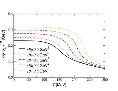
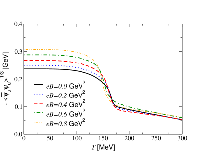
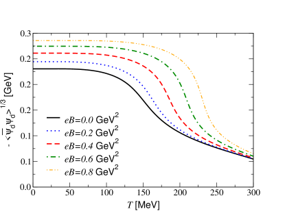
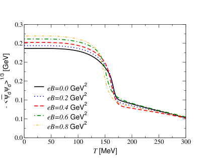
Figure 1: Quark condensate for flavors $u$ and $d$ as functions of temperature for different values of the magnetic field for $G$ (left) and $G(B,T)$ (right).

We start describing the fitting procedure used to obtain the thermo-magnetic dependence of the NJL coupling constant. Our strategy is to reproduce with the model the lattice results of Ref. fodor for the quark condensate average, $(\Sigma_{u}+\Sigma_{d})/2$. In the lattice calculation, the condensates are normalized in a way which is reminiscent of Gell-Mann–Oakes–Renner relation (GOR), $2m\langle\bar{\psi}_{f}\psi_{f}\rangle=m_{\pi}^{2}f_{\pi}^{2}+\dots$, as

$$\Sigma_{f}(B,T)=\frac{2m}{m_{\pi}^{2}f_{\pi}^{2}}\left[\langle\bar{\psi}_{f}\psi_{f}\rangle_{BT}-\langle\bar{\psi}_{f}\psi_{f}\rangle_{00}\right]+1,$$ (20)

with $\langle\bar{\psi}_{f}\psi_{f}\rangle_{00}$ representing the quark condensates at $T=0$ and $B=0$. In order to fit the lattice results, the other physical quantities appearing in Eq. (20) should be those of Ref. fodor ; namely, $m_{\pi}=135\;{\rm MeV}$, $f_{\pi}=86\;{\rm MeV}$, and $m=5.5\;{\rm MeV}$ so that, by invoking the GOR relation, one can use the LQCD value $\langle\bar{\psi}_{f}\psi_{f}\rangle_{00}^{1/3}=-230.55\,{\rm MeV}$. Therefore, as far as Eq. (20) is concerned, only $\langle\bar{\psi}_{f}\psi_{f}\rangle_{BT}$ is to be evaluated with the NJL model. As we show below, the NJL predictions for the in vacuum scalar condensate are numerically very close to those obtained with the LQCD simulations so that the above value for $\langle\bar{\psi}_{f}\psi_{f}\rangle_{00}$ can be safely used in Eq. (20) without introducing important uncertainties.

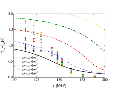
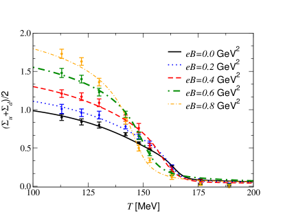
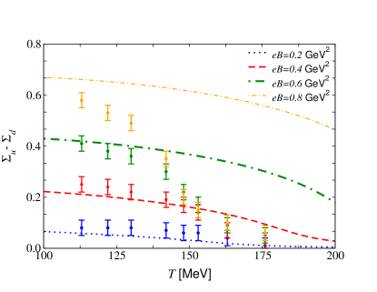
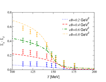
Figure 2: Condensate average and difference as functions of temperature for different values of the magnetic field for $G$ (left) and $G(B,T)$ (right). Data from Ref. fodor .

The LQCD results of Ref. fodor were obtained at $T=0$ and at high $T$, with no data points between $T=0$ and $T=113\leavevmode\nobreak\ {\rm MeV}$. Therefore, recalling that the discrepancies between lattice results and effective models appear in the region where chiral symmetry is partially restored (crossover), it seems therefore reasonable to fit the NJL coupling constant within this region and then to extrapolate the results to zero temperature if needed.

A good finite temperature fit to the lattice data for the average $(\Sigma_{u}+\Sigma_{d})/2$ can be obtained by using the following interpolation formula for NJL coupling constant:

$$G(B,T)=c(B)\left[1-\frac{1}{1+e^{\beta(B)\left[T_{a}(B)-T\right]}}\right]+s(B).$$ (21)

Note that the parameters $c,s,\beta$ and $T_{a}$ depend only on the magnetic field; their values are shown in Table 1. Remark also that Eq. (21) does not necessarily require the knowledge of $G(0,0)$, but one still needs $\Lambda$ and $m$ which in this work are taken at standard values, $\Lambda=0.650\leavevmode\nobreak\ {\rm GeV}$ and $m=5.5\leavevmode\nobreak\ {\rm MeV}$. This particular expression is taken simply for convenience; any other form that fits the data is expected to give the same qualitative results for thermodynamical quantities in the appropriate $B$ and $T$ range.

Table 1: Values of the fitting parameters in Eq. (21). Units are in appropriate powers of GeV.

$eB$	$c$	$T_{a}$	$s$	$\beta$
0.0	0.900	0.168	3.731	40.000
0.2	1.226	0.168	3.262	34.117
0.4	1.769	0.169	2.294	22.988
0.6	0.741	0.156	2.864	14.401
0.8	1.289	0.158	1.804	11.506

Figures 1 and  2 display the results for combinations of the quark condensates: the $u$ and $d$ condensates, their sum and difference. In the left panels of the figures, the condensates are evaluated with a $T-$ and $B-$independent coupling $G$ that fits the lattice results for the average $(\Sigma_{u}+\Sigma_{d})/2$ in vacuum, $G=4.50373\leavevmode\nobreak\ {\rm GeV}^{-2}$; in the right panels, the condensates are calculated with the coupling $G(B,T)$ of Eq. (21), with the fitting parameters given in Table 1.

The figures clearly show that the NJL model is able to capture the sharp decrease around the crossover temperature of the lattice results for the average and difference of the condensates only when the coupling $G(B,T)$ is used; when using the $T-$ and $B-$independent coupling $G$, a rather smooth behavior for these quantities is obtained. We have not attempted to obtain a $G(B,T)$ that gives a best fit for both $(\Sigma_{u}+\Sigma_{d})/2$ and $\Sigma_{u}-\Sigma_{d}$, but one sees that the model nevertheless gives a very reasonable description of the latter. Although here we are not particularly concerned with the results at $T=0$, for the sake of completeness we mention that an extrapolation of the fit to $T=B=0$ gives $G(0,0)=4.6311\leavevmode\nobreak\ {\rm GeV}^{-2}$. Such a coupling leads to $\langle{\bar{\psi}}_{f}\psi_{f}\rangle^{1/3}_{00}=-236.374\leavevmode\nobreak\ {\rm MeV}$, which differs only by a few percent from the value calculated with $G$. This small discrepancy is due to the fact that we have attempted to obtain a good fit with a limited number of parameters of the lattice data at high temperatures only, where more data are available.

3 Thermodynamical quantities

In the present section we examine the predictions of the NJL model for the thermodynamical quantities of magnetized quark matter when the fitted coupling $G(B,T)$ is used. We start by considering the quantities that characterize the equation of state (EoS), such as the normalized pressure $P_{N}=P(T,B)-P(0,B)$, the entropy density $s$, the energy density $\cal E$, and the EoS parameter $P_{N}/{\cal E}$. These quantities are displayed in Figures 3 and 4 for the $T-$ and $B-$independent $G$ and $G(B,T)$ couplings. We note that the choice to present results for $P_{N}$, instead for $P(T,B)$ and $P(0,B)$ in separate, is for presentation convenience; $P_{N}$ vanishes at $T=0$ and the explicit dependence of the term $B^{2}/2$ cancels in the difference.

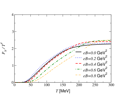
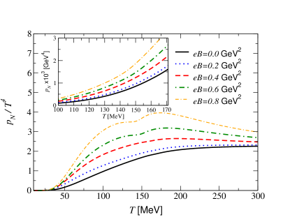
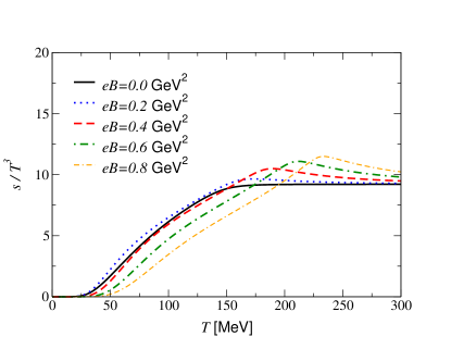
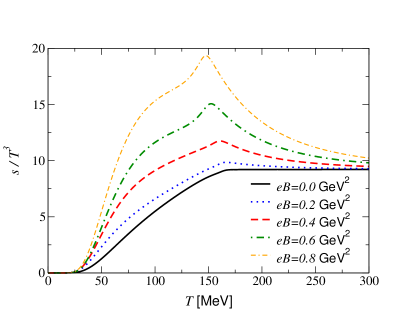
Figure 3: Normalized pressure and entropy density as functions of temperature for different values of the magnetic field calculated with $G$ (left) and $G(B,T)$ (right).

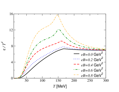
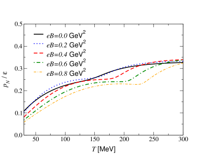
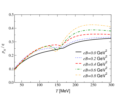
Figure 4: Energy density and equation of state as functions of temperature for different values of the magnetic field calculated with $G$ (left) and $G(B,T)$ (right).

A first observation is that $G(B,T)$ always predicts larger values for $P_{N}$, $s$, and $\cal E$ for a given temperature as the field strength increases as compared to the corresponding values obtained with a $T-$ and $B-$independent coupling $G$. Moreover, qualitative different $T$ dependences at high and low temperature values can be observed by comparing the two top panels of Fig. 3. Starting with the left panel, which corresponds to $G$, one observes that the pressure value decreases as $B$ increases at very low temperatures ($T\lesssim 50\,{\rm MeV}$) while an opposite trend is observed at high temperatures ($T\gtrsim 250\,{\rm MeV}$). One also observes that at intermediate temperatures ($T\simeq 200\,{\rm MeV}$) the pressure values predicted by increasingly higher fields oscillate around the $B=0$ value. On the other hand, the top right panel corresponding to $G(B,T)$ predicts that a higher field always leads to a higher pressure. The $G(B,T)$ coupling also predicts a more dramatic increase of the pressure around the chiral crossover; at $eB=0.8\;{\rm GeV}^{2}$, the pressure predicted with $G(B,T)$ is about twice the value at $B=0$, while the departure from the $B=0$ curve is more modest in the case when $G$ is considered.

The NJL predictions with a $G(B,T)$ for thermodynamical observables can be contrasted with recent lattice results bali . For example, the systematic increase of $P_{N}$ with $B$ is clearly observed in Fig. 5 of Ref. bali while the behavior of $P_{N}/\epsilon$ seen in Fig. 7 of the same reference is similar to the one found in Fig. 3 and Fig. 4 of the present paper. We remark that a different normalization has been used in Ref. bali and, at first sight, our results for $P_{N}/T^{4}$ seem to contradict those in the latter reference, but this is not so; the inset in Fig. 3 shows that, for a given $T$, the pressure always increases with $B$, like in the left panel of Fig. 7 in Ref. bali . Our results for $s/T^{3}$ and ${\cal E}/T^{4}$ also predict a sharper transition and so the peaks are more pronounced than the ones which appear at fixed $G$. Even more important is the fact that, for increasing $B$, the peaks occur at lower temperatures, in a clear indication of IMC. Finally, notice that although the lattice calculations of Ref. bali are for $2+1$ flavors, a qualitative agreement can clearly be noticed. We emphasize once more that the results with fixed $G$ present a clear discrepancy with the ones obtained within the LQCD simulations of Ref. bali .

Before investigating other thermodynamical quantities, let us recall that the crossover temperature, or the pseudo-critical temperature $T_{pc}$, for which chiral symmetry is partially restored, is usually defined as the temperature at which the thermal susceptibility

$$\chi_{T} = -m_{\pi}\frac{\partial\sigma}{\partial T}\,,$$ (22)

$$\sigma = \frac{\langle\bar{\psi}_{u}\psi_{u}\rangle(B,T)+\langle\bar{\psi}_{d}\psi_{d}\rangle(B,T)}{\langle\bar{\psi}_{u}\psi_{u}\rangle(B,0)+\langle\bar{\psi}_{d}\psi_{d}\rangle(B,0)},$$ (23)

reaches a maximum. Note that we have followed the usual LQCD definition which includes the pion mass in the definition of $\chi_{T}$ to make it a dimensionless quantity. As in the previous section, we again consider $m_{\pi}=135\;\leavevmode\nobreak\ {\rm MeV}$.

Fig. 5 displays $\chi_{T}$ and $c_{v}$, and Fig. 6 displays $c_{s}^{2}$ and $\Delta$. As in the previous cases, we observe an overall enhancement of all quantities in the transition region for strong magnetic fields while the Stefan-Boltzmann limit is approached as the temperature increases.

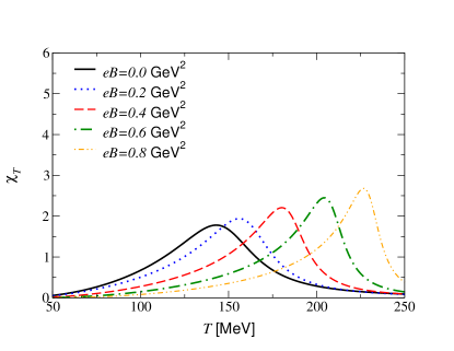
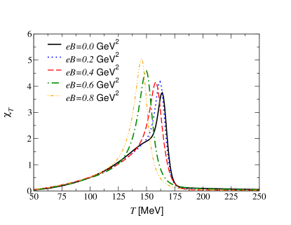
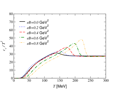
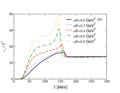
Figure 5: The thermal susceptibility and specific heat as functions of temperature for different values of the magnetic field obtained with $G$ (left) and $G(B,T)$ (right).

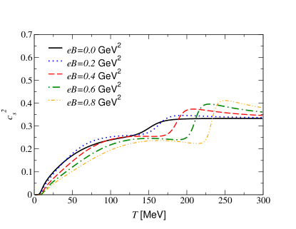
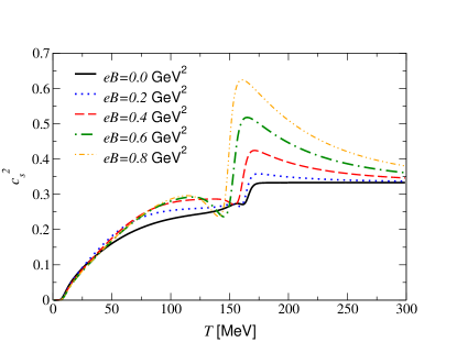
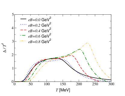
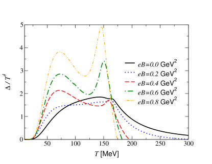
Figure 6: The sound velocity squared and interaction measure as functions of temperature for different values of the magnetic field obtained with $G$ (left) and $G(B,T)$ (right).

The results clearly indicate that the thermal susceptibility changes dramatically when $G$ is replaced by $G(B,T)$. In particular, one notices in Fig. 6 that $\Delta$ presents peaks that move in the direction of low temperatures when $B$ increases, in accordance with Ref. bali . Remark that the maxima that appear at low (and intermediate) values of $T$ are due the parametrization of the model, because the value of the coupling that fits the lattice results at $T=B=0$ is $10\,\%$ smaller than the usual value for the model jpcsGB0 . As we have verified, using this value of $G$ that fits the lattice results, the shape for $\Delta$ is deformed for small (intermediate) values of $T$, but since this region has not yet been explored by LQCD simulations, we cannot draw further conclusions at this point. At this point it is important to emphasize that the critical temperature for vanishing $B$ defined as the value, $T_{pc}$, where the thermal susceptibility reaches a peak does not coincide with the critical temperature found by lattice simulations. This discrepancy shows up for instance on the top right panel of Fig.5 for the case of $B=0$. Effective models do not reproduce the same lattice values for $T_{pc}$ at $B=0$ and, usually, most authors linearly rescale the temperature axis so that their results match the lattice inflection point at $B=0$. In our case we do not rescale the temperature axis, the lattice results are given at $B=T=0$. We perform our fitting at the critical region extrapolating the results for $T=0$ as well as high-$T$ so that our predictions for $T_{pc}$, at $B=0$, are slightly different from those obtained by LQCD.

The dependence of the pseudocritical temperature on the magnetic field strength is displayed in Fig. 7, which shows that when $G(B,T)$ is used, the phenomenon of IMC is observed to occur in a manner consistent with LQCD predictions. In this figure we define $T_{pc}$ using the thermal susceptibility $\chi_{T}$ and the specific heat $c_{v}$; we also include the temperatures of the maxima of interaction measure $\Delta$ to investigate its displacement with increasing $B$. It is interesting to remark that although this peak appears at a temperature which is a little higher than $T_{pc}$, it approximately follows the behavior of magnetic thermal susceptibility.

Finally, let us consider the magnetization which, in our case, can be written as

$${\cal M}=\frac{dP}{dB}=\frac{\partial P}{\partial B}+\frac{\partial P}{\partial M}\frac{\partial M}{\partial B}+\frac{\partial P}{\partial G}\frac{\partial G}{\partial B},$$ (24)

but, the quark masses are obtained by the gap equation $\partial P/{\partial M}=0$, so that the second term vanishes. Notice that a linear term, arising from the $B^{2}/2$ contribution to the pressure, has been neglected so as to normalize $\cal M$ to vanish at zero temperature. Therefore,

$${\cal M} = \frac{\partial}{\partial B}\left(P_{u}+P_{d}\right)+\frac{(M-m)^{2}}{4G^{2}}\frac{\partial G}{\partial B}.$$ (25)

Since the vacuum part of the pressure do not depend on $B$, they do not contribute to the magnetization. The derivatives of the pressure are

$$\frac{\partial P^{mag}_{f}}{\partial B} = \frac{2P^{mag}_{f}}{B}-\frac{N_{c}|q_{f}|}{4\pi^{2}}M^{2}\biggl{[}\ln\Gamma(x_{f})-\frac{1}{2}\ln(2\pi)$$ (26)

$$+ x_{f}-\left(x_{f}-\frac{1}{2}\right)\ln(x_{f})\biggr{]}\,,$$

$$\frac{\partial P^{Tmag}_{f}}{\partial B} = \frac{P_{f}^{Tmag}}{B}$$ (27)

$$\,-\frac{N_{c}|q_{f}|^{2}B}{2\pi^{2}}\sum_{k=0}^{\infty}k\alpha_{k}\int_{-\infty}^{+\infty}dp\frac{n(E_{f})}{E_{f}}.$$

The magnetization, Eq. (25), is readily obtained from the expressions given in Sec. II for the pressure. The remaining derivatives are easily calculated.

In Fig. 8 we show the normalized magnetization ${\cal M}/e$ as a function of temperature for different magnetic field strengths. Again, one observes that a fixed coupling $G$ does not predict a monotonic increase of the magnetization with $eB$ for a given temperature. This can be observed more clearly in Fig. 9 where we show how the pressure and magnetization depend on $eB$ at a fixed temperature, $T=70$ MeV. While the traditional fixed coupling predicts a magnetization that becomes negative as the magnetic field strength is increased, the thermo-magnetic coupling yields to positive magnetizations and is in agreement to the paramagnetic nature of thermal QCD medium observed in $N_{f}=2+1$ LQCD simulations of Ref. bali .

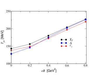
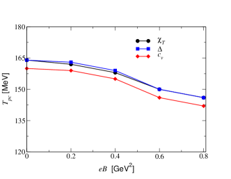
Figure 7: The pseudocritical temperature for the chiral transition of magnetized quark matter as a function of the magnetic field strength obtained with $G$ (left) and with $G(B,T)$ (right).

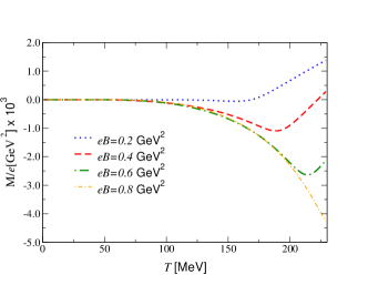
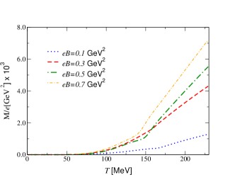
Figure 8: The normalized magnetization $M/e$ of quark matter as a function of the temperature for different values of the magnetic field strength obtained with $G$ (left) and $G(B,T)$ (right).

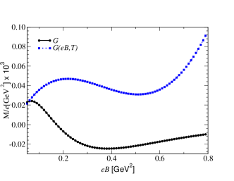
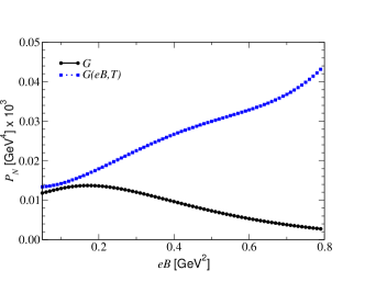
Figure 9: The normalized magnetization $M/e$ (left) and the normalized pressure (right) as a function of the magnetic field at $T=70$ MeV, obtained with $G$ (solid line) and $G(B,T)$ (dotted line).

We close this section by remarking that, to the best of our knowledge, LQCD predictions for the $N_{f}=2$ case analyzed here are not available in the literature. Although one could argue that the use of a three flavor version of the NJL model would be more appropriate to compare with lattice results, we recall that our ansatz for the four-fermion interaction strength, $G$, was obtained by fitting the LQCD results for the light quark sector, which represents the relevant degrees of freedom regarding the chiral transition. Using this fit, one retrieves, at least qualitatively, most of the lattice predictions for different thermodynamical quantities for the $N_{f}=2+1$ case, improving over predictions made with a fixed coupling. Remark that a more sophisticated $SU(3)$ NJL model possesses a six-fermion vertex characterized by another coupling, $K$, tailored to account for strangeness, and has been adopted for realistic astrophysical applications, where strangeness is important, or comparisons aiming at quantitative agreement with $N_{f}=2+1$ LQCD predictions for thermodynamical observables. In principle, $K$ can also be considered to have a thermo-magnetic dependence and then with this extra degree of freedom one could attempt to obtain a numerically more accurate description of the LQCD results for $N_{f}=2+1$ as a (more appropriate) alternative to the simple approach considering solely the $G$ coupling, with a magnetic dependence only prdferreira . In a forthcoming work, we will show the thermo-magnetic dependencies $G(B,T)$ and $K(B,T)$ obtained by fitting the mean and difference of $u$ and $d$ quark condensates computed in the framework of LQCD. While finishing our paper we have learned of a similar implementation of $G(B,T)$ in Ref. ayalafit

4 Conclusions

We have investigated the thermodynamics of magnetized quark matter within the NJL model using a coupling $G$ that decreases with both the temperature $T$ and the magnetic field $B$. The $T$ and $B$ dependence of $G$ was obtained by an accurate fit of lattice QCD results for the light-quark condensates. Using the fitted $G(B,T)$, we computed different thermodynamical quantities and analyzed the qualitative changes implied by the fitted coupling. The main conclusion of our work is that a coupling $G(B,T)$ that fits lattice result for $T_{pc}$ as determined by the quark condensates, gives results for the pressure, entropy and energy densities that are in qualitative agreement with corresponding lattice results, while a $B-$ and $T-$independent coupling gives qualitatively different results for those quantities. In particular, for any fixed temperature, quantities such as pressure and magnetization obtained with $G(eB,T)$ increase with $eB$, a result that is consistent with lattice QCD results.

Here, we have shown a very important result: NJL model calculations performed with our thermo-magnetic coupling predicts that the magnetization is positive in all temperature range, which complies to the paramagnetic nature of QCD medium and is in agreement with lattice calculations. Another feature that supports the thermo-magnetic dependence of the coupling constant is the observation that the chiral transition seems sharper and peaks observed in quantities such as the entropy density increase considerably with $eB$, a feature that is also consistent with lattice simulations and often missed when using a $B-$ and $T-$independent coupling. As remarked earlier, the results seem to indicate that the $B$ and $T$ dependence in $G$ that gives the correct $T_{pc}$ is neither fortuitous nor valid for a single physical quantity only; it seems to capture correctly the physics left out in the conventional NJL model. Also, any interpolation formula of the lattice data points for the quark condensate is expected to give qualitatively similar results for the thermodynamical quantities in the appropriate range of $T$ and $B$.

Our results indicate that it is crucial to take into account both $B$ and $T$ effects in the effective coupling. First, it is virtually impossible to fit lattice results with an effective NJL coupling that depends on $B$; a coupling that depends on $B$, despite decreasing with $B$, leads prdferreira to non monotonic decrease of $T_{pc}$ at $eB\approx 1.1\,{\rm GeV}^{2}$. It is well known that in QCD the temperature also represents an energy scale and the coupling constant runs with $T$ when $B=0$. Therefore, in principle, purely thermal effects should also influence the NJL coupling – and of course, the same is expected for six-fermion or higher-order NJL couplings. However, in practice, with few exceptions bernard ; marcus , purely thermal effects are usually neglected since no qualitative discrepancies between lattice and model predictions have been observed so far when $T\neq 0$ and $B=0$, in contrast to the case when $B\neq 0$. Indeed, our results show that to have a consistent monotonic decrease of $T_{pc}$ with $B$, it is crucial to consider a $B-T$ dependent coupling, which seems to be consistent with the findings of Ref. bruno , where the authors of that reference argue that chiral models with couplings depending solely on $B$ are unable to correctly describe IMC. Also, in Ref. mao . IMC is observed when a thermo-magnetic effective coupling appears as a consequence of improving on a mean field evaluation with mesonic effects. Obviously, the model itself cannot explain the basic physics behind the required $B$ and $T$ dependence of the effective coupling, but it seems consistent with a physical interpretation based on competing effects between quark and gluon charges, as demonstrated in the one-loop vertex correction calculated in Ref. ayala7 . Naturally, other interpretations are not excluded and further work is required to clarify the physical picture.

In summary, we have shown that the NJL model can be patched in order to accurately reproduce IMC which is observed to take place within the chiral transition of hot and magnetized quark matter. In particular, the thermo-magnetic dependent coupling Eq. (21) seems to provide an appropriate effective coupling $G(B,T)$ that captures effects beyond the conventional NJL models and which can be promptly employed to improve predictions to hadronic systems involving large magnetic fields. The apparent weak dependence on $eB$ is essential to obtain a positive magnetization while the sharp dependence on $T$ ensures a good description of the chiral phase transition.

Acknowledgments

We thank G. Endrodi for discussions and also for providing the lattice data of the up and down quark condensates, and A. Ayala for useful comments on an earlier version of the manuscript. M. B. P. is also grateful to E. S. Fraga for useful comments. This work was supported by CNPq grants 475110/2013-7, 232766/2014-2, 308828/2013-5 (R.L.S.F), 306195/2015-1 (VST), 307458
/2013-0 (SSA), 303592/2013-3 (MBP), 305894/2009-9 (GK), FAPESP grants 2013/01907-0 (GK), 2016/07061-3 (VST) and FAEPEX grant 3284/16 (VST). R.L.S.F. acknowledges the kind hospitality of the Center for Nuclear Research at Kent State University, where part of this work has been done.

References

- (1) K. Fukushima, D. E. Kharzeev, and H. J. Warringa, Phys. Rev. D 78, 074033 (2008).
- (2) D. E. Kharzeev and H. J. Warringa, Phys. Rev. D 80, 0304028 (2009).
- (3) R. Duncan and C. Thompson, Astron. J., 32, L9 (1992); C. Kouveliotou et al., Nature 393, 235 (1998).
- (4) V. A. Miransky and I. A. Shovkovy, Phys. Rept. 576, 1 (2015).
- (5) J.O. Andersen, W.R. Naylor, and A. Tranberg, Rev. Mod. Phys. 88, 025001 (2016).
- (6) K. Tuchin, Adv. High Energy Phys. 2013, 490495 (2013); Phys. Rev. C 88, 024911 (2013).
- (7) L. McLerran and V. Skokov, Nucl. Phys. A 929, 184 (2014).
- (8) D.M. Sedrakian, D. Blaschke, Astrophysics 45,166 (2002); Astrofiz. 45, 203 (2002).
- (9) D. Blaschke, D.M. Sedrakian, K.M. Shahabasian, ASP Conf. Ser. 202, 607 (2000).
- (10) G. S. Bali, F. Bruckmann, G. Endrödi, Z. Fodor, S. D. Katz, S. Krieg, A. Schäfer, and K. K. Szabó, JHEP 1202, 044 (2012).
- (11) G. S. Bali, F. Bruckmann, G. Endrödi, Z. Fodor, S. D. Katz, and A. Schäfer, Phys. Rev. D 86, 071502(R) (2012).
- (12) E. S. Fraga and L. F. Palhares, Phys. Rev. D 86, 016008 (2012).
- (13) K. Fukushima and Y. Hidaka, Phys. Rev. Lett. 110, 031601 (2013).
- (14) T. Kojo and N. Su, Phys. Lett. B720, 192 (2013).
- (15) F. Bruckmann, G. Endrodi, and T. G. Kovacs, JHEP 1304, 112 (2013).
- (16) E.S. Fraga, J. Noronha, and L.F. Palhares, Phys. Rev. D 87, 114014 (2013).
- (17) Y. Sakai, T. Sasaki, H. Kouno, and M. Yahiro, Phys. Rev. D 82, 076003 (2010); ibid J. Phys. G 39, 035004 (2012).
- (18) T. Sasaki, Y. Sakai, H. Kouno, and M. Yahiro, Phys. Rev. D 84, 091901(R) (2011).
- (19) K. Fukushima, M. Ruggieri, and R. Gatto, Phys. Rev. D 81, 114031 (2010).
- (20) M. Ferreira, P. Costa, D. P. Menezes, C. Providência, and N. Scoccola, Phys. Rev. D 89, 016002 (2014).
- (21) E.S. Fraga, B.W. Mintz, and J. Schaffner-Bielich, Phys. Lett. B731, 154 (2014).
- (22) C. Bonati, M. D’Elia, M. Mariti, M. Mesiti, F. Negro, and F. Sanfilippo, Phys. Rev. D 89, 114502 (2014).
- (23) A. Ayala, L. A. Hernández, A. J. Mizher, J. C. Rojas, and C. Villavicencio, Phys. Rev. D 89, 116017 (2014) .
- (24) M. Ferreira, P. Costa, and C. Providência, Phys. Rev. D 90, 016012 (2014).
- (25) A. Ayala, M. Loewe, A.J. Mizher, and R. Zamora , Phys. Rev. D 90, 036001 (2014).
- (26) A. Ayala , M. Loewe, and R. Zamora, Phys. Rev. D 91, 016002 (2015).
- (27) E. J. Ferrer, V. de la Incera, and X. J. Wen, Phys. Rev. D 91, 054006 (2015).
- (28) G. Cao, L. He, and P. Zhuang, Phys. Rev. D 90, 056005 (2014).
- (29) Sh. Fayazbakhsh and N. Sadooghi, Phys. Rev. D 90, 105030 (2014).
- (30) J. O. Andersen, W. R. Naylor, and A. Tranberg, JHEP 1502, 042 (2015).
- (31) K. Kamikado and T. Kanazawa, JHEP 1501, 129 (2015).
- (32) A. Ayala, J. J. C. Martínez, M. Loewe, M. E. T. Yeomans, and R. Zamora, Phys. Rev. D 91, 016007 (2015).
- (33) G. Endrödi, PoS LATTICE2014, 018 (2014).
- (34) L. Yu, J. V. Doorsselaere, and M. Huang, Phys. Rev. D 91, 074011 (2015).
- (35) B. Feng, De-fu Hou, and Hai-cang Ren, Phys. Rev. D 92, 065011 (2015).
- (36) J. Braun, W. A, Mian, and S. Rechenberger, arXiv:1412.6025 [hep-ph].
- (37) N. Mueller and J. M. Pawlowski, Phys. Rev. D 91, 116010 (2015).
- (38) A. Ayala, C.A. Dominguez, L.A. Hernandez, M. Loewe, J.C. Rojas, and C. Villavicencio, Phys. Rev. D 92, 016006 (2015).
- (39) G. Endrödi, JHEP 1507, 173 (2015).
- (40) D. P. Menezes and L. L. Lopes, Eur. Phys. J. A 52, 17 (2016).
- (41) R. Rougemont, R. Critelli, and J. Noronha, Phys. Rev. D 93, 045013 (2016).
- (42) R. Z. Denke and M. B. Pinto, arXiv:1506.05434 [hep-ph].
- (43) D. P. Menezes, M. B. Pinto, and C. Providência, Phys. Rev. C 91, 065205 (2015).
- (44) P. Costa, M. Ferreira, D. P. Menezes, J. Moreira, and C. Providência, Phys. Rev. D 92, 036012 (2015).
- (45) A. Ayala, C.A. Dominguez, L.A. Hernández, M. Loewe, and R. Zamora, Phys. Rev. D 92, 119905 (2015), Erratum Phys. Rev. D 92, 119905 (2015).
- (46) G. Cao and X. G. Huang, Phys. Rev. D 93, 016007 (2016).
- (47) R. Yoshiike and T. Tatsumi, Phys. Rev. D 92, 116009 (2015).
- (48) K. Hattori, T. Kojo, and Nan Su, Nucl. Phys. A 951, 1 (2016).
- (49) B. Feng, D. Hou , H.C. Ren, and P.P. Wu, Phys. Rev. D 93, 085019 (2016).
- (50) G. Cao, A. Huang , Phys. Rev. D 93, 076007 (2016).
- (51) C.F. Li, L. Yang, X.J. Wen, and G.X. Peng, Phys. Rev. D 93, 054005 (2016).
- (52) A. Ahmad and A. Raya, J. Phys. G, 065002 (2016).
- (53) V. Bernard and U.G. Meissner, Annals Phys. 206, 50 (1991).
- (54) M. B. Pinto, Phys. Rev. D 50, 7673 (1994).
- (55) R.L.S. Farias, K.P. Gomes, G. Krein, and M.B. Pinto, Phys. Rev. C 90, 025203 (2014).
- (56) M. Ferreira, P. Costa, O. Lourenço, T. Frederico, and C. Providência, Phys. Rev. D 89, 116011 (2014).
- (57) A. Ayala, C.A. Dominguez, L.A. Hernandez, M. Loewe, and R. Zamora, Phys. Let. B 759, 99 (2016).
- (58) Y. Nambu and G. Jona-Lasinio, Phys. Rev. 122, 345 (1961).
- (59) D. Ebert and K. G. Klimenko, Nucl. Phys. A 728, 203, (2003).
- (60) D. P. Menezes, M. B. Pinto, S. S. Avancini, A. P. Martínez, and C. Providência, Phys. Rev. C 79, 035807, (2009).
- (61) P. G. Allen, A. G. Grunfeld, and N. N. Scoccola, Phys. Rev. D 92, 074041, (2015).
- (62) D.C. Duarte, P. G. Allen, R.L.S. Farias, P.H.A. Manso, R.O. Ramos, and N. N. Scoccola, Phys. Rev. D 93, 025017 (2016).
- (63) S.S. Avancini, W.R. Tavares and M. B. Pinto, Phys. Rev. D 93, 014010 (2016).
- (64) S.S. Avancini, R.L.S. Farias, M.B. Pinto, W.R. Tavares and V.S. Timóteo, Phys. Lett. B 767, 247 (2017).
- (65) S.P. Klevansky, Rev. Mod. Phys. 64, 649 (1992).
- (66) M. Buballa, Phys. Rep. 407, 205 (2005).
- (67) G. N. Ferrari, A. F. Garcia, and M. B. Pinto, Phys. Rev. D 86, 096005 (2012).
- (68) J. K. Boomsma and D. Boer, Phys. Rev. D 81, 074005 (2010).
- (69) G. S. Bali, F. Bruckmann, G. Endrödi, S. D. Katz, and A. Schäfer, JHEP 1408, 177 (2014).
- (70) R. L. S. Farias, V. S. Timóteo, S. Avancini, M. B. Pinto, G. Krein, J. Phys. Conf. Ser. 706 (2016), 052029.
- (71) A. Ayala, C.A. Dominguez, L.A. Hernandez, M. Loewe, A. Raya, J.C. Rojas, and C. Villavicencio, Phys. Rev. D 94, 054019 (2016).
- (72) S. Mao, Phys.Lett. B758, 195 (2016).