One-way Quantum Deficit and Decoherence for Two-qubit $X$ States

Abstract

We study one-way quantum deficit of two-qubit $X$ states systematically from analytical derivations. An effective approach to compute one-way quantum deficit of two-qubit $X$ states has been provided. Analytical results are presented as for detailed examples. Moreover, we demonstrate the decoherence of one-way quantum deficit under phase damping channel.

Keywords One-way quantum deficit; two-qubit $X$ states; decoherence

I Introduction

Quantum entanglement is one of the most distinguishing properties in quantum mechanics, which gives quantum information processing novel advantages over classical information processing hhhh ; horodecki09 . Recently, quantum correlations modi12 receive much attention because they may play vital roles in quantum information processing and quantum simulation even without quantum entanglement datta08 ; lanyon08 . The characterization and quantification of quantum correlations have become one of the significant topics in the past decade modi12 . One of the quantum correlations is characterized by quantum discord zurek01 ; henderson01 which is shown to play important roles in quantum information tasks such as quantum state discrimination roa11 ; libo12 , remote state preparation da12 and quantum state merging maca ; cavalcanti11 . There have been many kinds of quantum correlations like measurement-induced disturbance luo2 , geometric quantum discord daluo ; luo10 , relative entropy of discord modi , continuous-variable discord adesso ; giorda etc.. However, analytical computation of these quantum correlations seem extremely difficult as optimization involved. Few analytical results have been obtained even for general two-qubit states. An analytical formula of quantum discord for Bell-diagonal states is provided in luo08 . For general two-qubit $X$ states, the analytical formula is still missed ali10 ; lu11 ; chen11 ; davi ; huang13 . Recently, the authors in loa ; yur ; yur15 presented a better classification in deriving analytical quantum discord for five parameters $X$ states.

Among other quantum correlations, the quantum deficit is related to extract work from a correlated system coupled to a heat bath under nonlocal operations opp02 , with the work deficit defined by $W_{t}-W_{l}$, where $W_{t}$ is the information of the whole system and $W_{l}$ is the localizable information horo05 . It is also equal to the difference of the mutual information and the classical deficit oppenheim2 . The analytical formula of one-way quantum deficit opp02 ; horo05 , like quantum discord, remains unknown. In Ref.wyk the quantum deficit of four-parameter two-qubit $X$ states has been calculated. Numerical results for five-parameter $X$ states are presented in Ref.wyk14 . In this paper, by using different approaches, we systematically compute the one-way quantum deficit for general two-qubit $X$ states in terms of analytical derivations. Analytical results are presented for classes of detailed quantum states. Decoherence of one-way quantum deficit under phase damping channels is calculated too.

II One-way quantum deficit of two-qubit $X$ states

We consider two-qubit states $\rho_{AB}$ in Hilbert space $\mathcal{H}_{A}^{2}\otimes\mathcal{H}_{B}^{2}$. The one-way quantum deficit str11 is defined according to the minimal increase of entropy after measurement on $B$,

$$\tilde{\Delta}(\rho_{AB})=\min_{M_{k}}S(\sum_{k}M_{k}\rho_{AB}M_{k})-S(\rho_{AB}),$$ (1)

where the minimum is taken over all measurement operators $\{M_{k}\}$ satisfying $\sum_{k}M_{k}=\mathbbm{1}$, $S(\rho)=-{\rm Tr}\rho\log_{2}\rho$ is von Neumann entropy. It is equal to the thermal discord zurek03 . It is also denoted by the relative entropy to the set of classical-quantum states horo05 .

Since the quantum correlations between $A$ and $B$ do not change under the local unitary operations, we consider $\rho_{AB}$ in the Bloch representation as

$$\rho_{AB}=\frac{1}{4}[I\otimes I+x\sigma_{3}\otimes I+yI\otimes\sigma_{3}+\sum_{i=1}^{3}t_{i}\sigma_{i}\otimes\sigma_{i}],$$ (2)

where $\sigma_{i}$ $(i=1,2,3)$ are the Pauli matrices, $x,y,t_{1},t_{2}$ and $t_{3}$ are real number. Equivalently under the computational bases $\{|00\rangle,|01\rangle,|10\rangle,|11\rangle\}$,

$$\rho_{AB}=\left(\begin{array}[]{cccc}a&0&0&f\cr 0&b&e&0\cr 0&e&c&0\cr f&0&0&d\end{array}\right),$$ (7)

where

$$a = \frac{1}{4}\left(1+t_{3}+x+y\right);~{}~{}~{}b=\frac{1}{4}\left(1-t_{3}+x-y\right);$$ (8)

$$c = \frac{1}{4}\left(1-t_{3}-x+y\right);~{}~{}~{}d=\frac{1}{4}\left(1+t_{3}-x-y\right);$$ (9)

$$e = \frac{1}{4}\left(t_{1}+t_{2}\right);~{}~{}~{}~{}~{}~{}~{}~{}~{}~{}~{}~{}~{}f=\frac{1}{4}\left(t_{1}-t_{2}\right).$$ (10)

$\rho_{AB}$ is called two-qubit $X$ state, in which the parameters satisfy the relations $a,b,c,d,e,f\geq 0$, $a+b+c+d=1$, $|e|^{2}\leq bc$ and $|f|^{2}\leq ad$.

It is easily verified that $S(\rho_{AB})$ in (1) is given by $S(\rho_{AB})=-\sum_{\pm}(u_{\pm}\log_{2}u_{\pm}+v_{\pm}\log_{2}v_{\pm})$, with

$$u_{\pm} =\frac{1}{4}(1+t_{3}\pm\sqrt{(x+y)^{2}+(t_{1}-t_{2})^{2}}),$$

$$v_{\pm} =\frac{1}{4}(1-t_{3}\pm\sqrt{(x-y)^{2}+(t_{1}+t_{2})^{2}}).$$ (11)

For arbitrary rank-two two-qubit states, the projective measurements are optimal to minimizes the von Neumann entropy shi . They are also almost sufficient rank-three and four two-qubit states galve11 . In the following, we focus on projective measurements. Let $M_{k}$ be the local measurement operators on subsystem $B$, $M_{k}=V\Pi_{k}V^{\dagger}$, with $\Pi_{k}=|k\rangle\langle k|$, $k=0,1$, and $V\in U(2)$ unitary matrices. Generally $V$ can be expressed as $V=tI+i\vec{y}\cdot\vec{\sigma}$, where $t\in R$ and $\vec{y}=(y_{1},y_{2},y_{3})\in R^{3}$ satisfy $y_{1}^{2}+y_{2}^{2}+y_{3}^{2}+t^{2}=1$. After measurement the state $\rho_{AB}$ is transformed to the ensemble $\{\rho_{k},p_{k}\}$ with

$$\rho_{k}=\frac{1}{p_{k}}(I\otimes M_{k})\,\rho_{AB}\,(I\otimes M_{k}),$$ (12)

and $p_{k}={\rm tr}(I\otimes M_{k})\rho_{AB}(I\otimes M_{k})$. By tedious calculation wyk14 , we have $\sum_{k}(I\otimes M_{k})\,\rho_{AB}\,(I\otimes M_{k})=p_{0}\rho_{0}+p_{1}\rho_{1}$, where

$$p_{0}\rho_{0} = \frac{1}{4}[I+yz_{3}I+t_{1}z_{1}\sigma_{1}+t_{2}z_{2}\sigma_{2}+(x+t_{3}z_{3})\sigma_{3}]\otimes V\Pi_{0}V^{\dagger},$$ (13)

$$p_{1}\rho_{1} = \frac{1}{4}[I-yz_{3}I-t_{1}z_{1}\sigma_{1}-t_{2}z_{2}\sigma_{2}-(x-t_{3}z_{3})\sigma_{3}]\otimes V\Pi_{1}V^{\dagger},$$ (14)

$z_{1}=2(-ty_{2}+y_{1}y_{3})$, $z_{2}=2(ty_{1}+y_{2}y_{3})$, $z_{3}=t^{2}+y_{3}^{2}-y_{1}^{2}-y_{2}^{2}$.

From the matrix diagonalization techniques in Ref. wyk , we have the eigenvalues of $\sum_{k}(I\otimes M_{k})\,\rho_{AB}\,(I\otimes M_{k})$,

$$\lambda_{1,2}=\frac{1}{4}\left(1+yz_{3}\pm\sqrt{(x+t_{3}z_{3})^{2}+t_{1}^{2}z_{1}^{2}+t_{2}^{2}z_{2}^{2}}\right),$$

$$\lambda_{3,4}=\frac{1}{4}\left(1-yz_{3}\pm\sqrt{(x-t_{3}z_{3})^{2}+t_{1}^{2}z_{1}^{2}+t_{2}^{2}z_{2}^{2}}\right),$$ (15)

with $z_{1}^{2}+z_{2}^{2}+z_{3}^{2}=1$. Therefore the one-way quantum deficit (1) is given by

$$\tilde{\Delta}=\sum_{\pm}(u_{\pm}\log_{2}u_{\pm}+v_{\pm}\log_{2}v_{\pm})+\min[-\sum_{i=1}^{4}\lambda_{i}\log_{2}\lambda_{i}].$$ (16)

To find the analytical solutions of (16), let us set $z_{1}=\sin\theta\cos\varphi$, $z_{2}=\sin\theta\sin\varphi$ and $z_{3}=\cos\theta$. Then

$$\lambda_{1,2}=\frac{1}{4}\left(p_{+}\pm\sqrt{R+S_{+}}\right),~{}~{}~{}~{}\lambda_{3,4}=\frac{1}{4}\left(p_{-}\pm\sqrt{R+S_{-}}\right),$$ (17)

where

$$p_{\pm}=1\pm y\cos\theta,~{}~{}~{}\\ R=[t_{1}^{2}\cos^{2}\varphi+t_{2}^{2}\sin^{2}\varphi]\sin^{2}\theta,~{}~{}~{}\\ S_{\pm}=\left(x\pm t_{3}\cos\theta\right)^{2}.$$

Because $\lambda_{i}$ is the eigenvalue of the density matrix, $\lambda_{i}\geqslant 0$. Hence $p_{\pm}\geqslant\sqrt{R+S_{\pm}}\geqslant 0$.

Denote $G(\theta,\varphi)=-\sum_{i=1}^{4}\lambda_{i}\log_{2}\lambda_{i}$. The one-way quantum deficit is given by the minimal value of $G(\theta,\varphi)$. We observe that $G(\theta,\varphi)=G(\pi-\theta,\varphi)$ and $G(\theta,\varphi)=G(\theta,2\pi-\varphi)$. Moreover, $G(\theta,\varphi)$ is symmetric with respect to $\theta=\pi/2$ and $\varphi=\pi$. Therefore, we only need to consider the case of $\theta\in[0,\pi/2]$ and $\varphi\in[0,\pi)$.

The extreme points of $G(\theta,\varphi)$ are determined by the first partial derivatives of $G$ with respect to $\theta$ and $\varphi$,

$$\frac{\partial G}{\partial\theta}=-\frac{\sin\theta}{4}H_{\theta},$$ (18)

with

$$H_{\theta}= \frac{R\csc\theta\cot\theta-t_{3}\sqrt{S_{+}}}{\sqrt{R+S_{+}}}\log_{2}\frac{p_{+}+\sqrt{R+S_{+}}}{p_{+}-\sqrt{R+S_{+}}}+y\log_{2}\frac{p_{-}^{2}-(R+S_{-})}{p_{+}^{2}-(R+S_{+})}$$ (19)

$$+\frac{R\csc\theta\cot\theta+t_{3}\sqrt{S_{-}}}{\sqrt{R+S_{-}}}\log_{2}\frac{p_{-}+\sqrt{R+S_{-}}}{p_{-}-\sqrt{R+S_{-}}},$$

and

$$\frac{\partial G}{\partial\varphi}=2\,ef\sin^{2}\theta\,\sin 2\varphi\,H_{\varphi},$$ (20)

with

$$H_{\varphi}=\frac{1}{\sqrt{R+S_{+}}}\log_{2}\frac{p_{+}+\sqrt{R+S_{+}}}{p_{+}-\sqrt{R+S_{+}}}+\frac{1}{\sqrt{R+S_{-}}}\log_{2}\frac{p_{-}+\sqrt{R+S_{-}}}{p_{-}-\sqrt{R+S_{-}}}.$$ (21)

Since $H_{\varphi}$ is always positive, $\frac{\partial G}{\partial\varphi}=0$ implies that either $\sin 2\varphi=0$, namely, $\varphi=0,\pi/2,$ for any $\theta$, or $\theta=0$ for any $\varphi$ which implies that (18) is zero at the same time and the minimization is independent on $\varphi$. If $\theta\neq 0$, one gets the second derivative $\partial^{2}G/\partial\varphi^{2}$

$$\frac{\partial^{2}G}{\partial\varphi^{2}}|_{(\theta,0)} =4ef\sin^{2}(\theta)H_{\varphi=0}>0,$$ (22)

and

$$\frac{\partial^{2}G}{\partial\varphi^{2}}|_{(\theta,\pi/2)} =-4ef\sin^{2}(\theta)H_{\varphi=\pi/2}<0.$$ (23)

Since for any $\theta$ the second derivative $\partial^{2}G/\partial\varphi^{2}$ is always negative for $\varphi=\pi/2$, we only need to deal with the minimization problem for the case of $\varphi=0$. To minimize $G(\theta,\varphi)$ becomes to minimize $G(\theta,0)$ which can be written as $G(\theta,0)=-\sum_{j,k=1}^{2}w_{j,k}\log_{2}w_{j,k}$ with

$$w_{j,k=1,2}=\frac{1}{4}\left(1+(-1)^{j}y\cos(\theta)+(-1)^{k}\sqrt{t_{1}^{2}\sin^{2}(\theta)+\left(x+(-1)^{j}t_{3}\cos(\theta)\right){}^{2}}\right).$$ (24)

The derivative (18) is zero for either $\sin\theta=0$ or $H_{\theta}=0$. $\sin\theta=0$ gives an extreme point $\theta=\theta_{e}=0$. While $H_{\theta}=0$ has the one obvious solution $\theta_{e}=\pi/2$ and a special solution $\theta_{s}$ that depends on the density matrix entries. The optimization problem is then reduced to study the second derivative of $G(\theta,0)$ with respect to $\theta$ evaluated at the critical angles $\theta_{e}=0,\pi/2$ and $\theta_{s}$. Denote $H_{\theta}^{\prime}=\partial H_{\theta}/\partial\theta$. The second derivative $\partial^{2}G/\partial^{2}\theta=-(\cos\theta\,H_{\theta}+\sin\theta\,H_{\theta}^{\prime})/4$ evaluated at the three $\theta_{e}$s depends on the behavior of two quantities,

$$H_{0}= -\partial^{2}G/\partial^{2}\theta|_{\theta=0}$$

$$= \frac{t_{1}^{2}-t_{3}|x+t_{3}|}{|x+t_{3}|}\log_{2}\frac{p_{+}+|x+t_{3}|}{p_{+}-|x+t_{3}|}+y\log_{2}\frac{p_{-}^{2}-(x-t_{3})^{2}}{p_{+}^{2}-(x+t_{3})^{2}}$$ (25)

$$+\frac{t_{1}^{2}+t_{3}|x-t_{3}|}{|x-t_{3}|}\log_{2}\frac{p_{-}+|x-t_{3}|}{p_{-}-|x-t_{3}|},$$

and

$$H_{\pi/2}^{\prime}= -\partial^{2}G/\partial^{2}\theta|_{\theta=\pi/2}$$

$$= -4[(t_{3}^{2}x^{2}+(y^{2}-2t_{3}xy)(t_{1}^{2}+x^{2}))\sqrt{t_{1}^{2}+x^{2}}$$

$$+ t_{1}^{2}\left(t_{1}^{2}+x^{2}-1\right)\left(t_{1}^{2}-t_{3}^{2}+x^{2}\right)\tanh^{-1}\left(\sqrt{t_{1}^{2}+x^{2}}\right)]/[(t_{1}^{2}+x^{2}-1)(t_{1}^{2}+x^{2}){}^{3/2}].$$ (26)

The sign of $H_{0}$ and $H_{\pi/2}^{\prime}$ determines which of $G(0,0)$, $G(\pi/2,0)$ and $G(\theta_{s},0)$ is the minimum.

(1) If $H_{0}>0$ and $H_{\pi/2}^{\prime}>0$, then $\theta_{s}$ takes values in $(0,\pi/2)$. In this case, the minimum of $G(\theta_{s},0)$ depends on the state. For given $\rho_{AB}$, $\theta_{s}$ can be calculated numerically from $H_{\theta}=0$.

(2) Otherwise, we have the minimum either $G(0,0)$ or $G(\pi/2,0)$,

$$G(0,0)=-\sum_{k,j\in\{0,1\}}Q_{k,j}\log_{2}Q_{k,j},$$ (27)

with $Q_{k,j}=\frac{1}{4}[(1+(-1)^{k}x)+(-1)^{j}(y+(-1)^{k}t_{3})]$, and

$$G(\pi/2,0)=1+\mathcal{L}(\frac{1}{2}\left(1-\sqrt{t_{1}^{2}+x^{2}}\right)),$$ (28)

where $\mathcal{L}(w)=-w\log_{2}w-(1-w)\log_{2}(1-w)$ is the binary entropy. Thus, we have the following result: one-way quantum deficit of $\rho_{AB}$ is given by

$$\tilde{\Delta}=\sum_{\pm}(u_{\pm}\log_{2}u_{\pm}+v_{\pm}\log_{2}v_{\pm})+G,$$ (29)

where

$$G=\left\{\begin{array}[]{ll}G(\theta_{s},0),&\hbox{$H_{0}>0$ and $H_{\pi/2}^{\prime}>0$, $\theta_{s}\in(0,\pi/2)$};\\ \min\{G(0,0),G(\pi/2,0)\},&\hbox{others}.\end{array}\right.$$ (30)

By careful numerical analysis, there is at most one zero point of first derivative of $G(\theta,0)$ with respect to $\theta$, and only when $H_{0}>0$ and $H_{\pi/2}^{\prime}>0$, one gets the minimum inside the interval $\theta_{s}\in(0,\pi/2)$. Therefore, we can obtain the analytical minimum of $G$ at $\theta=0,\pi/2$ or $\theta=\theta_{s}$. In the following we present some detailed examples.

Example 1. Consider the class of special $X$ states defined by

$$\rho_{AB}=q|\psi^{-}\rangle\langle\psi^{-}|+(1-q)|00\rangle\langle 00|,$$ (31)

where $|\psi^{-}\rangle=\frac{1}{\sqrt{2}}(|01\rangle-|10\rangle)$, $q\in[0,1]$.

By using the Bloch sphere representation, from (II) and (II) we have

$$H_{0}(q)=\frac{(q-1)}{\left|2-3q\right|}\left[\left|2-3q\right|\log_{2}\left(\frac{2}{q}-2\right)+(5q-2)\log_{2}\left(\frac{q-2+\left|2-3q\right|}{q-2-\left|2-3q\right|}\right)\right]$$ (32)

and

$$H_{\pi/2}^{\prime}=\frac{4(1-q)}{\left(2q^{2}-2q+1\right)^{3/2}}\left(\sqrt{2q^{2}-2q+1}\left(4q^{2}-3q+1\right)-2q^{3}\tanh^{-1}\left(\sqrt{2q^{2}-2q+1}\right)\right).$$ (33)

The case that both $H_{0}(q)>0$ and $H_{\pi/2}^{\prime}(q)>0$ happens only in interval $q\in(1/2,0.67)$, see Fig.1, where $q=1/2$ and $0.67$ are the solutions of $H_{0}(q)=0$ and $H_{\pi/2}^{\prime}=0$, respectively. From (29), we have

$$\tilde{\Delta}=\left\{\begin{array}[]{ll}q,&~{}~{}~{}\hbox{$\theta=0$, $q\in[0,1/2]$;}\\ G(\theta_{s},0),&~{}~{}~{}\hbox{$q\in(1/2,0.67]$;}\\[2.84526pt] q\log_{2}q+(1-q)\log_{2}(1-q)+1+\mathcal{L}(\frac{\left(1+\sqrt{q^{2}+(1-q)^{2}}\right)}{2}),&~{}~{}~{}\hbox{$\theta=\pi/2$, $q\in(0.67,1$],}\end{array}\right.$$ (37)

see Fig.1.

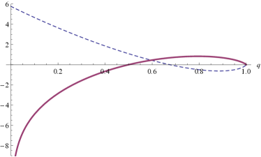
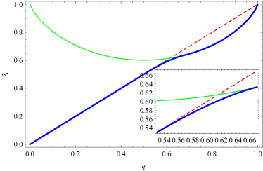
Figure 1: (a) $H_{0}$ (purple thick solid line) and $H_{\pi/2}^{\prime}$ (blue dashed line) with respect to $q$. (b) One-way quantum deficit (blue thick line) via $q$. The dashed red line stands for $G(0,0)$ which is the one-way quantum deficit for $q\in[0,1/2]$. The green line is for $G(\pi/2,0)$. It coincides with the one-way quantum deficit for $q\in(0.67,1$].

Example 2. We consider the state

$$\rho_{\alpha} =\alpha|\phi\rangle\langle\phi|+(1-\alpha)/2(|01\rangle\langle 01|+|10\rangle\langle 10|),$$ (38)

with $|\phi^{+}\rangle=(|00\rangle+|11\rangle)/\sqrt{2}$.

For this case we have

$$H_{0}(\alpha)=\frac{2(\alpha-1)(3\alpha-1)\left(\log_{2}\left(1-|2\alpha-1|\right)-\log_{2}\left(1+|2\alpha-1|\right)\right)}{|2\alpha-1|},$$ (39)

and

$$H_{\pi/2}^{\prime}=4(\alpha-1)(3\alpha-1)\tanh^{-1}(\alpha)/\alpha.$$ (40)

For $\alpha=1/3$ both $H_{0}(\alpha)$ and $H_{\pi/2}^{\prime}(\alpha)$ are equal to zero. There is no domain of $\alpha$ such that both $H_{0}>0$ and $H_{\pi/2}^{\prime}>0$, see Fig. 2. Hence we can easily obtain the analytical expression of one-way quantum deficit for $\rho_{\alpha}$,

$$\tilde{\Delta}=\left\{\begin{array}[]{ll}\alpha,&\hbox{$\theta=0$, $\alpha\in[0,1/3]$;}\\ 1+\alpha+\alpha\log_{2}\alpha+\frac{1}{2}\left[(1-\alpha)\log_{2}(1-\alpha)-(1+\alpha)\log_{2}(1+\alpha)\right],&\hbox{$\theta=\pi/2$, $\alpha\in(1/3,1]$,}\end{array}\right.$$ (43)

see Fig.2 for the analytical expression of one-way quantum deficit vs $\alpha$.

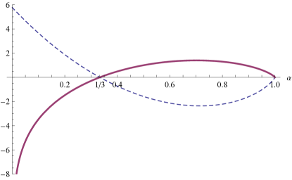
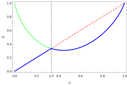
Figure 2: (a) $H_{0}$ (purple thick solid line) and $H_{\pi/2}^{\prime}$ (blue dashed line) with respect to $\alpha$. (b) One-way quantum deficit (blue thick line) via $\alpha$. Dashed red line for $G$ at $\theta=0$, and green line for $G$ at $\theta=\pi/2$.

Example 3. Consider the Bell diagonal state,

$$\rho_{AB}=\frac{1}{4}[I\otimes I+\sum_{i=1}^{3}t_{i}\sigma_{i}\otimes\sigma_{i}].$$ (44)

We have

$$H_{0}=\frac{2\left(t_{1}^{2}-t_{3}^{2}\right)}{|t_{3}|}\log_{2}\left(\frac{1+|t_{3}|}{1-|t_{3}|}\right)$$ (45)

and

$$H_{\pi/2}^{\prime}=-4\left(t_{1}^{2}-t_{3}^{2}\right)\tanh^{-1}\left(|t_{1}|\right)/|t_{1}|.$$ (46)

Since $\log_{2}\frac{1+|t_{3}|}{1-|t_{3}|}>0$ and $\tanh^{-1}\left(|t_{1}|\right)>0$, $H_{0}$ and $H_{\pi/2}^{\prime}$ cannot be greater than zero simultaneously. We obtain the analytical expression $\min\{G(0,0),G(\pi/2,0)\}$,

$$G(0,0)=1+\mathcal{L}(\frac{1+|t_{3}|}{2})$$ (47)

and

$$G(\pi/2,0)=1+\mathcal{L}(\frac{1+|t_{1}|}{2}).$$ (48)

Therefore $\min\{G(0,0),G(\pi/2,0)\}=1+\mathcal{L}(\frac{1+t}{2})$, where $t=\max\{|t_{1}|,|t_{3}|\}$. In fact, for Bell-diagonal states, the optimization is ontained at $t_{3}=\pm t_{1}$ or $t_{3}=\pm t_{2}$ chen11 . Therefore, we recovered the result in Ref.wyk where $t=\max\{|t_{1}|,|t_{2}|,|t_{3}|\}$.

III One-way quantum deficit under decoherence

A system undergoes environmental noises can be characterized by Kraus operators. We consider quantum two-qubit systems subjecting to dephasing channels described by the Kraus operators $F_{0}=|0\rangle\langle 0|+\sqrt{1-\gamma}|1\rangle\langle 1|$ and $F_{1}=\sqrt{\gamma}=|1\rangle\langle 1|$, where $\gamma=1-e^{-\tau t}$ and $\tau$ is phase damping rate nielsen . Under the channel the $\rho_{AB}$ is changed to be

$$\rho_{AB}^{\prime} =\sum_{i,j=0}^{1}F_{i}^{A}\otimes F_{j}^{B}\rho_{AB}(F_{i}^{A}\otimes F_{j}^{B})^{\dagger}$$

$$=\frac{1}{4}[I\otimes I+x\sigma_{3}\otimes I+yI\otimes\sigma_{3}+\sum_{i=1}^{2}(1-\gamma)^{2}t_{i}\sigma_{i}\otimes\sigma_{i}+(t_{3}\sigma_{3}\otimes\sigma_{3})].$$

We see that $t_{1}$ and $t_{2}$ have been transformed to $(1-\gamma)^{2}t_{1}$ and $(1-\gamma)^{2}t_{2}$. We have

$$H_{0}= -\partial^{2}G/\partial^{2}\theta|_{\theta=0}$$

$$= \frac{\Upsilon^{2}-t_{3}|x+t_{3}|}{|x+t_{3}|}\log_{2}\frac{p_{+}+|x+t_{3}|}{p_{+}-|x+t_{3}|}+y\log_{2}\frac{p_{-}^{2}-(x-t_{3})^{2}}{p_{+}^{2}-(x+t_{3})^{2}}$$ (49)

$$+\frac{\Upsilon^{2}+t_{3}|x-t_{3}|}{|x-t_{3}|}\log_{2}\frac{p_{-}+|x-t_{3}|}{p_{-}-|x-t_{3}|}$$

and

$$H_{\pi/2}^{\prime}= \Upsilon^{2}\left(\Upsilon^{2}+x^{2}-1\right)\left(\Upsilon^{2}-t_{3}^{2}+x^{2}\right)\tanh^{-1}\left(\sqrt{\Upsilon^{2}+x^{2}}\right)]/(\left(\Upsilon^{2}+x^{2}-1\right)\left(\Upsilon^{2}+x^{2}\right){}^{3/2})$$ (50)

$$-4[(-2t_{3}xy(\Upsilon^{2}+x^{2})+x^{2}y^{2}+\Upsilon^{2}y^{2}+t_{3}^{2}x^{2})\sqrt{\Upsilon^{2}+x^{2}},$$

where $\Upsilon=(1-\gamma)^{2}t_{1}$. It is direct to verify that $G(0,0)$ exactly given by (27). While $G(\pi/2,0)$ has the following form,

$$G(\pi/2,0)=1+\mathcal{L}(\frac{1}{2}\left(1-\sqrt{\Upsilon^{2}+x^{2}}\right)).$$ (51)

As an example, taking $x=0.45$, $y=0.32$, $t_{1}=0.43$, $t_{2}=0.09$ and $t_{3}=0.15$, we can observe the one-way quantum deficit under phase damping channel, see Fig. (3). It should be emphasized that the exact boundaries exist between three different branches and sudden transitions occur in the phase damping channel.

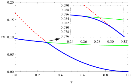
Figure 3: One-way quantum deficit vs $\gamma$ under dephasing noise for $x=0.45$, $y=0.32$, $t_{1}=0.43$, $t_{2}=0.09$ and $t_{3}=0.15$.

IV Summary

We have provided an effective approach to get analytical results of one-way quantum deficit for general two-qubit $X$ states. Analytical formulae of one-way quantum deficit have been obtained in general for states such that $\min\{G(0,0),G(\pi/2,0)\}$. It has been shown that only in very few cases, the conditions $H_{0}>0$ and $H_{\pi/2}^{\prime}>0$ are satisfied. Even in such special cases, the one-way quantum deficit can be easily calculated by solving $\theta_{s}$ from a one-parameter equation. We have also studied the decoherence of one-way quantum deficit under phase damping channel. As for a detailed example, it has been shown that the one-way quantum deficit changes gradually phase damping channel. There is no behavior like sudden death of quantum entanglement.

Acknowledgments    We thank the anonymous referee for the useful suggestions and valuable comments. This work is supported by the NSFC under number 11275131.

References

(1) Amico, L., Fazio, R., Osterloh, A., Vedral, V.: Rev. Mod. Phys. 80, 517 (2008)
(2)Horodecki, R., Horodecki, P., Horodecki, M.,
Horodecki, K.: Rev. Mod. Phys.
81, 865 (2009)
(3) Modi, K., Brodutch, A., Cable, H., Paterek, T.,
Vedral, V.: Rev. Mod. Phys. 84, 1655 (2012)
(4)
Datta, A., Shaji, A., Caves, C. M.: Phys. Rev. Lett. 100, 050502 (2008)
(5)
Lanyon, B. P., Barbieri, M., Almeida, M. P., White, A. G.: Phys. Rev.
Lett., 101, 200501 (2008)
(6) Ollivier, H., Zurek, W. H.: Phys. Rev.
Lett. 88, 017901(2001)
(7) Henderson, L., Vedral, V.:
J. Phys. A 34, 6899 (2001)
(8)
Roa, L., Retamal, J. C., Alid-Vaccarezza, M.: Phys. Rev. Lett. 107, 080401 (2011)
(9)
Li, B., Fei, S. M., Wang, Z. X., Fan, H.: Phys. Rev. A 85, 022328 (2012)
(10)
Daki¡äc, B., et al.: Nat. Phys. 8, 666 (2012)