Measurements of $d_{2}^{n}$ and $A_{1}^{n}$: Probing the neutron spin structure

Abstract

We report on the results of the E06-014 experiment performed at Jefferson Lab in Hall A, where a precision measurement of the twist-3 matrix element $d_{2}$ of the neutron ($d_{2}^{n}$) was conducted. The quantity $d_{2}^{n}$ represents the average color Lorentz force a struck quark experiences in a deep inelastic electron scattering event off a neutron due to its interaction with the hadronizing remnants. This color force was determined from a linear combination of the third moments of the ³He spin structure functions, $g_{1}$ and $g_{2}$, after nuclear corrections had been applied to these moments. The structure functions were obtained from a measurement of the unpolarized cross section and of double-spin asymmetries in the scattering of a longitudinally polarized electron beam from a transversely and a longitudinally polarized ³He target. The measurement kinematics included two average $Q^{2}$ bins of $3.2$ GeV² and $4.3$ GeV², and Bjorken-$x$ $0.25\leq x\leq 0.90$ covering the deep inelastic and resonance regions. We have found that $d_{2}^{n}$ is small and negative for $\left<Q^{2}\right>=3.2$ GeV², and even smaller for $\left<Q^{2}\right>=4.3$ GeV², consistent with the results of a lattice QCD calculation. The twist-4 matrix element $f_{2}^{n}$ was extracted by combining our measured $d_{2}^{n}$ with the world data on the first moment in $x$ of $g_{1}^{n}$, $\Gamma_{1}^{n}$. We found $f_{2}^{n}$ to be roughly an order of magnitude larger than $d_{2}^{n}$. Utilizing the extracted $d_{2}^{n}$ and $f_{2}^{n}$ data, we separated the Lorentz color force into its electric and magnetic components, $F_{E}^{y,n}$ and $F_{B}^{y,n}$, and found them to be equal and opposite in magnitude, in agreement with the predictions from an instanton model but not with those from QCD sum rules. Furthermore, using the measured double-spin asymmetries, we have extracted the virtual photon-nucleon asymmetry on the neutron $A_{1}^{n}$, the structure function ratio $g_{1}^{n}/F_{1}^{n}$, and the quark ratios $(\Delta u+\Delta\bar{u})/(u+\bar{u})$ and $(\Delta d+\Delta\bar{d})/(d+\bar{d})$. These results were found to be consistent with DIS world data and with the prediction of the constituent quark model but at odds with the perturbative quantum chromodynamics predictions at large $x$.

I Introduction

I.1 Overview of nucleon structure

Experiments utilizing the scattering of leptons from nucleons have been instrumental in uncovering the complex structure of subatomic matter over the past half century. In the mid-1950s, elastic scattering of electrons from hydrogen revealed that the proton is not a point-like particle but has internal structure Mcallister and Hofstadter (1956); in the 1970s, deep-inelastic scattering (DIS) of electrons from hydrogen showed that point-like particles, labeled “partons,” are the underlying constituents of the proton Bloom et al. (1969); *Breidenbach:1969kd. These partons were later identified as quarks and gluons in the modern theory of strong interactions, quantum chromodynamics (QCD) Gross and Wilczek (1973a); *Gross:1973ju; *Gross:1974cs.

Since the late 1970s, scattering of polarized lepton beams from polarized nucleons and polarized light nuclear targets (deuterium and ³He) has given us the opportunity to probe the spin structure of the nucleon encoded in the $g_{1}$ and $g_{2}$ spin-structure functions. In particular, worldwide DIS studies focusing on $g_{1}$ as a function of both Bjorken-$x$ and $Q^{2}$ allowed the determination of the fraction of the proton spin that is carried by the quarks Kuhn et al. (2009); Aidala et al. (2013) and by the gluons Adare et al. (2014); Adamczyk et al. (2015). Here, $x$ is interpreted as the fractional momentum of the parent nucleon carried by the struck quark in the infinite momentum frame, and $Q^{2}\equiv-q^{2}$ is the four-momentum transferred to the target squared.

Early theoretical work Shuryak and Vainshtein (1982a); *Jaffe:1989xx; *Jaffe:1990qh has shown that the $g_{1}(x,Q^{2})$ and $g_{2}(x,Q^{2})$ spin-structure functions contain information on quark-gluon correlations. These dynamical effects are accessible through the $Q^{2}$-variations of these functions beyond those of the calculable perturbative QCD (pQCD) radiative corrections Dokshitzer (1977); *Gribov:1972ri; *Altarelli:1977zs. In fact, they appear in an expansion of both the measured $g_{1}$ spin-structure function and its moments in $x$ in powers of $1/Q^{2}$, but only at higher order. In contrast, in the measured $g_{2}$ spin-structure function, quark-gluon interactions are accessible at leading order in a similar expansion and thus suffer no $1/Q^{2}$ suppression. This makes measurements of $g_{2}$ particularly sensitive and important for studying multi-parton correlations in the nucleon.

Studies of the moments in $x$ of spin-structure functions have resulted in fundamental tests of QCD like that of the Bjorken sum rule Bjorken (1966); *Bjorken:1969mm; here, not only do they offer an opportunity to test our understanding of pQCD beyond the simple partonic picture, but they also allow for measured observables to be tested against ab initio calculations of lattice QCD. While there is a wealth of data available for $g_{1}$, fewer data exist for $g_{2}$—especially in the valence region. This region provides the dominant contribution to higher moments. These moments are of interest because the contribution arising from the lower-$x$ region of integration, where the structure functions are unknown, is small. Thus these higher moments offer robust experimental results relevant for a comparison with lattice QCD, for example. Finally, it is worth noting that high-precision data of the $g_{1}$ nucleon structure function in the valence region of deep inelastic scattering—namely $x\geq 0.6$—are still sparse, and every new data set with good precision offers a real possibility to test nucleon models in a domain sensitive to those models’ parameters.

I.2 The $g_{2}$ structure function and quark-gluon correlations

While the polarized structure function $g_{2}$ has no clear interpretation in the quark-parton model Manohar (1992), it is known to contain quark-gluon correlations, and can be decomposed as:

$$g_{2}\left(x,Q^{2}\right)=g_{2}^{\text{WW}}\left(x,Q^{2}\right)+\bar{g}_{2}\left(x,Q^{2}\right),$$ (1)

where $\bar{g}_{2}$ is the component of $g_{2}$ that contains the quark-gluon correlations Jaffe (1990), given by Cortes et al. (1992):

$$\bar{g}_{2}\left(x,Q^{2}\right) = \int_{x}^{1}\frac{\partial}{\partial y}\left[\frac{m_{q}}{M}h_{T}\left(x,Q^{2}\right)+\xi\left(y,Q^{2}\right)\right]\frac{dy}{y}.$$ (2)

Here, $h_{T}$ denotes the transversity distribution in the nucleon Filippone and Ji (2001), $\xi$ the quark-gluon correlation function, $m_{q}$ the quark mass of flavor $q$ and $M$ the nucleon mass. The quantity $g_{2}^{\text{WW}}$ in Eq. 1 is the Wandzura-Wilczek term, which is fully determined from the knowledge of the $g_{1}$ structure function Wandzura and Wilczek (1977):

$$g_{2}^{\text{WW}}\left(x,Q^{2}\right) = -g_{1}\left(x,Q^{2}\right)+\int_{x}^{1}\frac{g_{1}\left(y,Q^{2}\right)}{y}dy.$$ (3)

Under the operator product expansion (OPE) Wilson (1969), one can access the effects of quark-gluon correlations via the third moment of a linear combination of $g_{1}$ and $g_{2}$:

$$d_{2}\left(Q^{2}\right) = 3\int_{0}^{1}x^{2}\bar{g}_{2}\left(x,Q^{2}\right)dx$$ (4)

$$= \int_{0}^{1}x^{2}\left[2g_{1}\left(x,Q^{2}\right)+3g_{2}\left(x,Q^{2}\right)\right]dx.$$

Because of the $x^{2}$-weighting, $d_{2}$ is particularly sensitive to the large-$x$ behavior of $\bar{g}_{2}$. The quantity $d_{2}$ is related to a specific twist-3 ($\tau=3$) matrix element consisting of local operators of quark and gluon fields Ehrnsperger et al. (1994); Filippone and Ji (2001); Burkardt (2013):

$$2MP^{+}P^{+}S^{x}d_{2} = g\langle P,S|\bar{\psi}(0)\gamma^{+}G^{+y}(0)\psi(0)|P,S\rangle,$$ (5)

where $P$ denotes the nucleon momentum, $S$ its spin, $\psi$ the quark field, and $g$ the QCD coupling constant. The $+$ superscript indicates the equation is expressed in light-cone coordinates. In analogy to the electromagnetic Lorentz force $F^{y}$ that acts on a charged particle, the gluon field $G^{+y}=\left(B^{x}-E^{y}\right)/\sqrt{2}=F^{y}$, where $B^{x}$ and $E^{y}$ are the transverse components of the color magnetic and color electric field, respectively; the $z$ direction is defined by the three-momentum transfer of the virtual photon Burkardt (2013).

There are two interpretations of $d_{2}$ in the literature. The first connects $d_{2}$ with color electromagnetic fields induced in a transversely polarized nucleon probed by a virtual photon. These induced color fields (appearing in Eq. 5) are represented as color polarizabilities $\chi$ Filippone and Ji (2001):

$$\chi_{E}\vec{S} = \frac{1}{2M^{2}}\langle P,S|\psi^{\dagger}g\vec{a}\times\vec{E}\psi|P,S\rangle$$ (6)

$$\chi_{B}\vec{S} = \frac{1}{2M^{2}}\langle P,S|\psi^{\dagger}g\vec{B}\psi|P,S\rangle,$$ (7)

where $\vec{a}$ denotes the velocity of the struck quark. Then, $d_{2}$ can be expressed as:

$$d_{2}=\frac{1}{4}\left(\chi_{E}+2\chi_{B}\right).$$ (8)

A second, more recent interpretation shows that the matrix element connected to $d_{2}$ represents an average color Lorentz force $F^{y}$ acting on the struck quark due to the remnant di-quark system at the instant it is struck by the virtual photon (cf. Eq. 5):

$$F^{y}(0) \equiv \langle P,S|\bar{\psi}(0)\gamma^{+}G^{+y}(0)\psi(0)|P,S\rangle$$ (9)

$$= -M^{2}d_{2},$$ (10)

where the last equality is true only in the rest frame of the nucleon Burkardt (2013).

Combining measurements of $d_{2}$ with the twist-4 matrix element $f_{2}$ allows the extraction of the color electric and magnetic forces $F_{E}^{y}$ and $F_{B}^{y}$ Burkardt (2013):

$$d_{2} = -\frac{1}{M^{2}}\left(F_{E}^{y}+F_{B}^{y}\right)$$ (11)

$$f_{2} = -\frac{2}{M^{2}}\left(2F_{E}^{y}-F_{B}^{y}\right).$$ (12)

The quantity $f_{2}$ is sensitive to quark-gluon correlations, since it is expressed as a matrix element similar to $d_{2}$, containing a mixed quark-gluon field operator Shuryak and Vainshtein (1982b, a); Edelmann et al. (2000); Osipenko et al. (2005). The $f_{2}$ matrix element cannot be measured directly, but can be extracted from $g_{1}$ data by utilizing a twist expansion of $\Gamma_{1}$, the first moment of $g_{1}$:

$$\Gamma_{1} \equiv \int_{0}^{1}g_{1}dx$$ (13)

$$= \mu_{2}+\frac{M^{2}}{9Q^{2}}\left(a_{2}+4d_{2}+4f_{2}\right)+\frac{\mu_{6}}{Q^{4}}$$

$$+ \mathcal{O}\left(\frac{1}{Q^{6}}\right)+\ldots.$$

For simplicity the $Q^{2}$-dependence of the structure functions, matrix elements and $\mu_{n}$ terms has been omitted in Eq. 13. The quantity $a_{2}=\int x^{2}g_{1}dx$ is the third moment of $g_{1}$, a twist-2 matrix element that has connections to target mass corrections. The term $\mu_{6}$ is a higher-twist ($\tau>4$) term. The quantity $\mu_{2}$ is the twist-2 contribution, given as:

$$\mu_{2}\left(Q^{2}\right)=C_{ns}\left(Q^{2}\right)\left(-\frac{1}{12}g_{A}+\frac{1}{36}a_{8}\right)+C_{s}\left(Q^{2}\right)\frac{1}{9}\Delta\Sigma,$$ (14)

where $C_{ns}$ and $C_{s}$ denote the non-singlet and singlet Wilson coefficients Larin et al. (1997), $g_{A}$ the flavor-triplet axial charge, $a_{8}$ the octet axial charge and $\Delta\Sigma\equiv\Delta\Sigma\left(Q^{2}=\infty\right)$, the renormalization group invariant definition of the singlet axial current. This definition of $\Delta\Sigma$ is used to factorize all of the $Q^{2}$ dependence into the Wilson coefficients, as was done in Refs. Osipenko et al. (2005); Meziani et al. (2005). The $f_{2}$ matrix element can be extracted from Eq. 13 by first subtracting $\mu_{2}$ from $\Gamma_{1}$ and then fitting the result as a function of $1/Q^{2}$.

In practice, in order to access the spin-structure functions $g_{1}$ and $g_{2}$, we measure experimental asymmetries:

$$A_{\parallel} \equiv \frac{\sigma^{\downarrow\Uparrow}-\sigma^{\uparrow\Uparrow}}{\sigma^{\downarrow\Uparrow}+\sigma^{\uparrow\Uparrow}}$$

$$= \frac{4\alpha^{2}}{MQ^{2}}\frac{(1-y)(2-y)}{2y^{2}\sigma_{0}}\times$$

$$\frac{(1-y)\sin\theta}{1+(1-y)\left[\cos\theta+\tan\left(\theta/2\right)\sin\theta\right]}\times$$

$$\left\{y\frac{1+(1-y)\cos\theta}{(1-y)\sin\theta}g_{1}-2\tan\left(\theta/2\right)g_{2}\right\}$$

$${\rm and}$$

$$A_{\perp} \equiv \frac{\sigma^{\downarrow\Rightarrow}-\sigma^{\uparrow\Rightarrow}}{\sigma^{\downarrow\Rightarrow}+\sigma^{\uparrow\Rightarrow}}$$

$$= \frac{4\alpha^{2}}{MQ^{2}}\frac{(1-y)(2-y)}{2y^{2}\sigma_{0}}\times$$

$$\frac{(1-y)\sin\theta}{1+(1-y)\left[\cos\theta+\tan\left(\theta/2\right)\sin\theta\right]}\times$$

$$\left\{yg_{1}+2g_{2}\right\}.$$

The quantity $\sigma^{sS}$ denotes the polarized cross section for electron spin $s$ and target spin $S$. The $\uparrow$ ($\downarrow$) indicates the electron spin parallel (antiparallel) to its momentum, and $\Uparrow$ ($\Downarrow$) indicates the target spin parallel (antiparallel) to the electron beam momentum. The $\Leftarrow$ ($\Rightarrow$) indicates the target spin perpendicular to the beam momentum, pointing away from (towards) the side of the beamline on which the scattered electron is detected. The quantity $y=(E-E^{\prime})/E$ is the fractional energy transferred to the target, with $E$ being the electron beam energy and $E^{\prime}$ the scattered electron energy, with $E$ and $E^{\prime}$ measured in the laboratory frame. The quantity $\alpha$ denotes the electromagnetic coupling constant and $\theta$ the electron scattering angle. The quantity $\sigma_{0}$ is the unpolarized electron scattering cross section. The dependence of $g_{1}$, $g_{2}$ and $\sigma_{0}$ on $x$ and $Q^{2}$ has been suppressed for simplicity.

The two spin structure functions $g_{1}$ and $g_{2}$ can be expressed in terms of the experimental observables $A_{\parallel}$, $A_{\perp}$ and $\sigma_{0}$ by combining and inverting Eqs. I.2 and I.2. Then the expression for $d_{2}$ in Eq. 4 can be re-written in terms of those experimental observables:

$$d_{2} = \int_{0}^{1}dx\frac{MQ^{2}}{4{\alpha}^{2}}\frac{x^{2}y^{2}}{\left(1-y\right)\left(2-y\right)}\sigma_{0}\times$$

$$\Bigg{[}\left(3\frac{1+\left(1-y\right)\cos\theta}{\left(1-y\right)\sin\theta}+\frac{4}{y}\tan\left(\theta/2\right)\right)A_{\perp}$$

$$+\left(\frac{4}{y}-3\right)A_{\parallel}\Bigg{]}.$$

The prior world data for $d_{2}^{n}$ as a function of $Q^{2}$  are presented in Fig. 1. The top panel shows measured data and model calculations without the elastic contribution, while the bottom panel shows the same data and models with the elastic contribution included. Resonance measurements from JLab E94-010 Amarian et al. (2004) and RSS Slifer et al. (2010), along with resonance plus DIS data from E01-012 Solvignon et al. (2015), are shown at $Q^{2}\lesssim 3$ GeV². At large $Q^{2}$ towards 5 GeV² are DIS measurements from SLAC E155x Anthony et al. (2003) and the combined data from JLab E99-117 and SLAC E155x Zheng et al. (2004a). In the latter data set, $d_{2}^{n}$ was evaluated by combining the $g_{2}^{n}$ data from JLab E99-117 with the $g_{2}$ data of SLAC E155x, and $\bar{g}_{2}$ was assumed to be $Q^{2}$-independent and to follow $\bar{g}_{2}\propto(1-x)^{m}$ with $m=2$ or 3 for $x\gtrsim 0.78$ Anthony et al. (2003), for which there were no data from either experiment Zheng et al. (2004a).

The solid curve in Fig. 1 is from a MAID Drechsel et al. (2007) calculation, which uses phenomenelogical fits to electro- and photoproduction data for the nucleon, extending from the single-pion production threshold to the resonance/DIS boundary at $W=2$ GeV. The major resonances are modeled using Breit-Wigner functions to construct the production channels. The bottom panel displays the results of additional model calculations from a QCD sum rule approach Stein et al. (1995a); Balitsky et al. (1990), which in general uses dispersion relations, combined with the OPE, to interpolate between the perturbative and non-perturbative regimes of QCD. The two calculations presented at $Q^{2}\approx 1$ GeV² use a three-quark field with Stein et al. (1995a) (offset lower in $Q^{2}$ in Fig. 1) and without Balitsky et al. (1990) a gluon field. A chiral soliton model Weigel et al. (1997); *Weigel:2000gx is shown, where the nucleon is described as a non-linear dynamical system consisting of “mesonic lumps” Weigel et al. (1997) governed by a $U(1)\times SU(2)_{L}\times SU(2)_{R}$ chiral symmetry. Another model displayed is a bag model, in which the quarks are confined to a nucleon “bag.” Here, the confinement mechanism of QCD is simulated using quark-gluon and gluon-gluon interactions Song (1996). The model also includes generalized spin-dependent effects via an explicit symmetry-breaking parameter Song and McCarthy (1994). A lattice QCD calculation Göckeler et al. (2005) is also presented, which solves the dynamical QCD equations non-perturbatively on a discretized lattice. The model calculations that include the elastic contribution are shown in the lower panel only. We added the elastic contribution to the MAID model in the lower panel. Our measurement focused on the moderately large-$Q^{2}$ region of $3<Q^{2}<5$ GeV², where the elastic contribution is seen to be small (lower panel of Fig. 1) and where a theoretical interpretation in terms of twist-3 contributions is cleaner.

While bag Song (1996); Stratmann (1993); Ji and Unrau (1994) and soliton Weigel et al. (1997); *Weigel:2000gx model calculations of $d_{2}$ for the neutron yield numerical values consistent with those of lattice QCD Göckeler et al. (2005), prior experimental data differ by roughly two standard deviations in the large $Q^{2}$-range. This is illustrated by the data for $Q^{2}\approx 5$ GeV² in Fig. 1. This situation called for a dedicated experiment for the neutron, JLab E06-014. For the proton $d_{2}$, the measurements and models are in better agreement Anthony et al. (2003); Stein et al. (1995a); Balitsky et al. (1990); Weigel et al. (1997); *Weigel:2000gx; Song (1996); Ji and Melnitchouk (1997); Göckeler et al. (2005). These data sets will be further extended by a recent measurement E07- (003) whose precision results are expected in the near future. Under the assumption of isospin symmetry, combining the neutron and proton data would then allow a flavor decomposition to determine the average color force felt by the up and down quarks in the proton. Measurements of $d_{2}$ access similar forces as those that cause quark confinement. Consequently, such measurements are important for understanding the dynamics of the constituents of the nucleon.

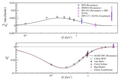
Figure 1: (Color online) The world $d_{2}^{n}$ data as a function of $Q^{2}$. Upper panel: Data and models without the elastic contribution. Bottom panel: Data and models with the elastic contribution included. The experimental resonance data from JLab E94-010 Amarian et al. (2004) and RSS Slifer et al. (2010), along with resonance plus DIS data from E01-012 Solvignon et al. (2015) are shown at $Q^{2}\lesssim 3$ GeV², while at larger $Q^{2}$ DIS data from SLAC E155x Anthony et al. (2003) and combined data from JLab E99-117 and SLAC E155x Zheng et al. (2004a) are shown. The solid curve is from a MAID Drechsel et al. (2007) calculation, which is dominated by the resonance contribution. Model calculations for $Q^{2}\approx 1$ GeV² from a QCD sum rule approach from Ref. Stein et al. (1995a) (offset lower in $Q^{2}$) and Ref. Balitsky et al. (1990) are shown. A chiral soliton model Weigel et al. (1997); *Weigel:2000gx and a bag model Song (1996) are also given. Additionally, a lattice QCD Göckeler et al. (2005) calculation is shown. The model calculations that include the elastic contribution are shown in the lower panel only. We added the elastic contribution to the MAID model in the lower panel. The elastic contribution to $d_{2}^{n}$ is given in the lower panel by the dashed curve, evaluated using the Cornwall-Norton (CN) moments (see Appendix B) where the Riordan Riordan et al. (2010) and Kelly Kelly (2004) parameterizations are used for $G_{E}^{n}$ and $G_{M}^{n}$, respectively.

Our measurements of the unpolarized cross section $\sigma_{0}$ and the double-spin asymmetries $A_{\parallel}$ and $A_{\perp}$ allow the extraction of $d_{2}$, and in turn, $f_{2}$. Combining our results for these higher-twist matrix elements, we obtain the color electric and magnetic forces $F_{E}^{y}$ and $F_{B}^{y}$. Utilizing our data on $g_{1}$, we also evaluate the twist-2 matrix element $a_{2}$ and test it against lattice QCD calculations.

I.3 $A_{1}$ and flavor decomposition

The measurement of the double-spin asymmetries $A_{\parallel}$ and $A_{\perp}$ required for the extraction of $d_{2}$ also gives access to the virtual photon-nucleon asymmetry $A_{1}$ and the polarized to unpolarized structure-function ratio $g_{1}/F_{1}$:

$$A_{1} = \frac{1}{D(1+\eta\xi)}A_{\parallel}-\frac{\eta}{d(1+\eta\xi)}A_{\perp}$$ (18)

$$\frac{g_{1}}{F_{1}} = \frac{1}{d^{\prime}}\left(A_{\parallel}+\tan\frac{\theta}{2}A_{\perp}\right),$$ (19)

where $F_{1}(x,Q^{2})$ denotes the unpolarized structure function and $D$ the virtual photon depolarization factor. This quantity, along with $\eta$, $d$, $\xi$ and $d^{\prime}$ are defined as:

$$D = \frac{E-\epsilon E^{\prime}}{E(1+\epsilon R)}$$ (20)

$$\eta = \frac{\epsilon\sqrt{Q^{2}}}{E-\epsilon E^{\prime}}$$ (21)

$$d = D\sqrt{\frac{2\epsilon}{1+\epsilon}}$$ (22)

$$\xi = \eta\frac{1+\epsilon}{2\epsilon}$$ (23)

$$d^{\prime} = \frac{(1-\epsilon)(2-y)}{y(1+\epsilon R)},$$ (24)

where $R\equiv\sigma_{L}/\sigma_{T}$, the ratio of longitudinally to transversely polarized photoabsorption cross sections . and $\epsilon$ denotes the ratio of the longitudinal to transverse polarization of the virtual photon:

$$\epsilon=\left[1+2\left(1+\gamma^{2}\right)\tan^{2}\frac{\theta}{2}\right]^{-1},$$ (25)

with $\gamma^{2}=\left(2Mx\right)^{2}/Q^{2}$.

The $A_{1}$ asymmetry is particularly sensitive to the way that the quark spins combine to give the nucleon spin. Therefore, $A_{1}$ is a good discriminator for various model calculations that aim to describe the spin structure of the nucleon. Figure 2 shows the previous world data using ³He targets from SLAC E142 Anthony et al. (1996) and E154 Abe et al. (1997a), HERMES Ackerstaff et al. (1997), and JLab E99-117 Zheng et al. (2004b, a) compared to various models. The SLAC E143 Abe et al. (1998) data, which used NH₃ and ND₃ targets, has been omitted from the plot due to their large uncertainties. It is seen that the relativistic constituent quark model (RCQM) Isgur (1999) describes the trend of the data reasonably well. The pQCD parameterization with hadron helicity conservation (HHC) Leader et al. (1998) (dashed)—assuming quark orbital angular momentum to be zero—does not describe the data adequately. However, the pQCD parameterization allowing for quark orbital angular momentum to be non-zero Avakian et al. (2007) (dash-dotted) is in good agreement with the data, suggesting the importance of quark orbital angular momentum in the spin structure of the nucleon. The statistical quark model (solid) Bourrely and Soffer (2015), which interprets the constituent partons as fermions (quarks) and bosons (gluons), adequately describes the trend of the world data after fitting its parameters to a subset of the available data. A modified NJL model from Cloët et al. (dash triple-dotted) Cloët et al. (2005) is shown to fit the data accurately in the large-$x$ region. This NJL-type model imposes constraints for confinement such that unphysical thresholds for nucleon decay into quarks are excluded. Nucleon states are obtained by solving the Faddeev equation using a quark-diquark approximation, including scalar and axial-vector diquark states. Relatively recent predictions come from Dyson-Schwinger Equation (DSE) treatments by Roberts et al. Roberts et al. (2013), which reveal non-pointlike diquark correlations in the nucleon due to dynamical chiral symmetry breaking. In these calculations Roberts et al. employ two different types of dressed-quark propagators for the Faddeev equation: one where the mass term is momentum-independent, and the other where the mass term carries a momentum dependence. This yields two different sets of results, referred to as contact and realistic, respectively. The predictions for the two approaches are shown at $x=1$ (Fig. 2). We note the contrast between the DSE predictions and those from pQCD and constituent quark models, where the latter two predict $A_{1}^{n}\rightarrow 1$ as $x\rightarrow 1$. The measurement presented here provides more contiguous coverage over the region of $0.27<x<0.60$ compared to the JLab E99-117 measurement Zheng et al. (2004b, a).

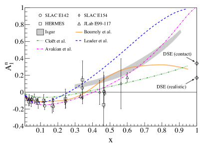
Figure 2: (Color online) World data for $A_{1}^{n}$ from SLAC E142 Anthony et al. (1996) and E154 Abe et al. (1997a), HERMES Ackerstaff et al. (1997), and JLab E99-117 Zheng et al. (2004b, a), compared to various models, including a pQCD-inspired global analysis (dashed) Leader et al. (1998), a statistical quark model from Bourrely et al. (solid) Bourrely and Soffer (2015), a pQCD parameterization including OAM from Avakian et al. (dash-dotted) Avakian et al. (2007) and a CQM model from Isgur (gray band) Isgur (1999). Also plotted is an NJL-type model from Cloët et al. (dash triple-dotted) Cloët et al. (2005). Predictions from Dyson-Schwinger Equation (DSE) treatments by Roberts et al. Roberts et al. (2013) are shown at $x=1$.

Even more than $A_{1}$, the polarized-to-unpolarized quark parton distribution function (PDF) ratios for the up quark ($u$), given by $\left(\Delta u+\Delta\bar{u}\right)/(u+\bar{u})$ and the down quark ($d$), given by $\left(\Delta d+\Delta\bar{d}\right)/(d+\bar{d})$, allow a high level of discrimination between theoretical models that describe the quark-spin contribution to nucleon spin. Such ratios may be extracted from measurements of $g_{1}/F_{1}$ at leading order in $Q^{2}$ according to:

$$\frac{\Delta u+\Delta\bar{u}}{u+\bar{u}} = \frac{4}{15}\frac{g_{1}^{p}}{F_{1}^{p}}\left(4+R^{du}\right)$$

$$-\frac{1}{15}\frac{g_{1}^{n}}{F_{1}^{n}}\left(1+4R^{du}\right)$$

$$\frac{\Delta d+\Delta\bar{d}}{d+\bar{d}} = \frac{4}{15}\frac{g_{1}^{n}}{F_{1}^{n}}\left(4+\frac{1}{R^{du}}\right)$$

$$-\frac{1}{15}\frac{g_{1}^{p}}{F_{1}^{p}}\left(1+4\frac{1}{R^{du}}\right),$$

where $R^{du}\equiv(d+\bar{d})/(u+\bar{u})$. Earlier experimental data for $(\Delta u+\Delta\bar{u})/(u+\bar{u})$ and $(\Delta d+\Delta\bar{d})/(d+\bar{d})$ are shown in Fig. 3, where the data in the upper (lower) part of the figure represent the up (down) quark ratio. The data shown are from HERMES Airapetian et al. (2005) and COMPASS Alekseev et al. (2010a), both semi-inclusive DIS measurements, and JLab experiments E99-117 Zheng et al. (2004a) and CLAS EG1b Dharmawardane et al. (2006), both of which are inclusive DIS measurements. The semi-inclusive DIS data from HERMES and COMPASS are constructed from their published polarized PDF data, where we used the same unpolarized PDF parameterizations as were applied in the original analyses: CTEQ5L Lai et al. (2000) for the HERMES data, and MRST2006 Martin et al. (2006) for the COMPASS data. The uncertainties are thus slightly larger than could be achieved from the raw data. The dashed curve represents a next-to-leading order (NLO) QCD global analysis that includes target mass corrections and higher-twist effects Leader et al. (2007), and the dashed-dotted curve represents a pQCD calculation that includes orbital angular momentum effects Avakian et al. (2007). The solid curve shows the statistical quark model Bourrely and Soffer (2015), and the dash triple-dotted curve is a modified NJL model Cloët et al. (2005). At $x=1$, DSE calculations Roberts et al. (2013) are indicated by open stars (crosses) for the up (down) quark ratios. Clearly, both pQCD models predict that $\Delta q/q\rightarrow 1$ at large $x$, which implies that the positive helicity state of the quark (quark spin aligned with the nucleon spin) must dominate as $x\rightarrow 1$. The data for $(\Delta u+\Delta\bar{u})/(u+\bar{u})$ are consistent with this prediction; however, we note that the current $(\Delta d+\Delta\bar{d})/(d+\bar{d})$ data show no sign of turning positive as we approach the large $x$ region. The Avakian et al. calculation fits the down quark data better, but still has a zero-crossing at $x\sim 0.75$. The data in Fig. 3 imply that in general, the up quark spins tend to be parallel to the nucleon spin, whereas the down quark spins are antiparallel to the nucleon spin. The trend of the down quark data, supported by the model of Avakian et al., suggests that quark orbital angular momentum might play an important role in the spin of the nucleon. The experiment presented here aims to provide more complete kinematic coverage for the down quark, especially in the large-$x$ region approaching $x\sim 0.6$, where the predictions of the pQCD models start to contrast with those of the constituent quark models and the DSE calculations.

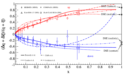
Figure 3: (Color online) The world data for the up and down quark polarized-to-unpolarized PDF ratios. The data shown are from HERMES Airapetian et al. (2005), a semi-inclusive DIS measurement, and JLab E99-117 Zheng et al. (2004a), and CLAS EG1b Dharmawardane et al. (2006), both of which are DIS measurements. Theoretical curves are from an NLO QCD analysis from Leader et al. Leader et al. (2007) (dashed) and pQCD-inspired fit from Avakian et al. Avakian et al. (2007) (dash-dotted). The solid curve shows a statistical quark model from Bourrely et al. Bourrely and Soffer (2015) and the dash triple-dotted curve shows a modified NJL model calculation from Cloët et al. Cloët et al. (2005). The open stars (crosses) at $x=1$ indicate the DSE calculations from Roberts et al. Roberts et al. (2013) for up (down) quarks.

I.4 Outline of the paper

The body of this paper is structured as follows: in Section II we discuss the experimental setup and the performance of the polarized electron beam and of the particle detectors for JLab E06-014; in Section III, we discuss the polarized ³He target; in Section IV, the data analysis to obtain the cross sections and asymmetries is presented. The nuclear corrections required to extract the neutron results for $d_{2}$, $a_{2}$, $A_{1}$ and $g_{1}/F_{1}$ are also discussed. In Section V the results of the experiment are presented. In particular, ³He results for the unpolarized cross section, double-spin asymmetries, $g_{1}$, $g_{2}$, $A_{1}$ and $g_{1}/F_{1}$ are given in Section V.1. In Section V.2 the results for the neutron $d_{2}$ and $a_{2}$ are presented. Following this, the analysis necessary to obtain the twist-4 matrix element $f_{2}$, leading to the extraction of the color forces $F_{E}^{y}$ and $F_{B}^{y}$ on the neutron, is discussed in Section V.2.3. The quantities $A_{1}$ and $g_{1}/F_{1}$ on the neutron are presented in Sections V.2.4 and V.2.5, respectively. The flavor separation analysis to obtain $(\Delta u+\Delta\bar{u})/(u+\bar{u})$ and $(\Delta d+\Delta\bar{d})/(d+\bar{d})$ is discussed and the results are presented in Section V.3. Concluding remarks are given in Section VI. Appendix A gives an overview of the DIS kinematics, structure functions and cross sections, while Appendix B discusses the details of the operator product expansion. Fits to unpolarized nitrogen cross sections and positron cross sections measured in this experiment, used in correcting the measured $e-^{3}$He cross section, are presented in Appendix C. Also presented in that appendix are fits to world proton data on $g_{1}/F_{1}$ and $A_{1}$, needed for the nuclear corrections. Details for the world $\Gamma_{1}^{n}$ data and fitting the higher-twist component of $\Gamma_{1}^{n}$ are given in Appendix D. The systematic uncertainties for all results presented in this paper are tabulated in Appendix E.

II The Experiment

The E06-014 experiment ran in Hall A of Thomas Jefferson National Accelerator Facility (Jefferson Lab or JLab) for six weeks in five run periods from February to March of 2009, consisting of a commissioning run using 1.2 GeV electrons, a 5.89 GeV run using polarized electrons, a 4.74 GeV run using unpolarized electrons, and finally runs using polarized electrons at energies of 5.89 GeV and 4.74 GeV. The data at 4.74 GeV and 5.89 GeV were the production data sets, which covered the resonance and deep inelastic valence quark regions, in a kinematic region of $0.25\leq x\leq 0.9$ and $2\text{ GeV}^{2}\leq Q^{2}\leq 6$ $\text{GeV}^{2}$, shown in Fig. 4.

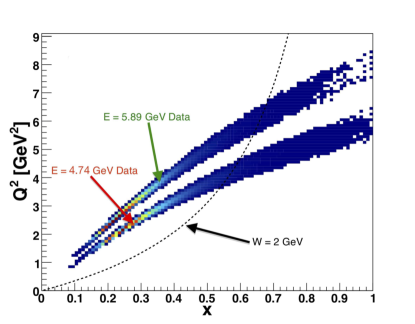
Figure 4: (Color online) The E06-014 kinematic coverage in $Q^{2}$ and $x$. The lower band represents the $E=4.74$ GeV data set and the upper band the $E=5.89$ GeV one. The black dashed line shows $W=2$ GeV. The regions to the left and right of this line correspond to DIS and resonance kinematics, respectively.

Polarized electrons were scattered from a polarized ³He target, which acts as an effective polarized neutron target Friar et al. (1990). The scattered electrons were detected independently in the Left High-Resolution Spectrometer (LHRS) and in the BigBite Spectrometer, that were oriented at a scattering angle of $\theta=45^{\circ}$ to the left and right of the beamline, respectively. The unpolarized cross section $\sigma_{0}$ was extracted from the LHRS data and the double-spin asymmetries $A_{\parallel}$ and $A_{\perp}$ were obtained from the BigBite data. The matrix element $d_{2}$ was computed using Eq. I.2, and the virtual photon asymmetry $A_{1}$ and structure function ratio $g_{1}/F_{1}$ were extracted according to Eqs. 18 and 19, respectively.

The measurement with the BigBite spectrometer consisted of twenty evenly spaced, continuous bins in $x$ with a bin width of 0.05 for each beam energy; of these, seven were discarded because of insufficient statistics. The statistics in all bins for a given beam energy were recorded simultaneously. The LHRS data were acquired in nine unevenly spaced bins in the scattered electron momentum $p$ for the $E=4.74$ GeV run and eleven unevenly spaced bins for the $E=5.89$ GeV run, covering a range of $0.6\leq p\leq 1.7$ GeV as listed in Tables 1 and 2. The statistics in the LHRS were recorded sequentially. For the $d_{2}$ extraction, the measured cross sections were interpolated and extrapolated to match the binning of the BigBite data.

Table 1: Kinematic bins for the LHRS for the 4.74 GeV run. The LHRS momentum setting is labeled as $p_{0}$.

$p_{0}$ $\left(\text{GeV}\right)$	$x$	$Q^{2}$ $\left(\text{GeV}^{2}\right)$
0.60	0.215	1.66
0.80	0.301	2.22
1.12	0.458	3.10
1.19	0.496	3.30
1.26	0.536	3.49
1.34	0.584	3.71
1.42	0.634	3.93
1.51	0.693	4.18
1.60	0.755	4.43

Table 2: Kinematic bins for the LHRS for the 5.89 GeV run. The LHRS momentum setting is labeled as $p_{0}$.

$p_{0}$ $\left(\text{GeV}\right)$	$x$	$Q^{2}$ $\left(\text{GeV}^{2}\right)$
0.60	0.209	2.07
0.70	0.248	2.42
0.90	0.332	3.11
1.13	0.437	3.90
1.20	0.471	4.14
1.27	0.506	4.38
1.34	0.542	4.62
1.42	0.584	4.90
1.51	0.634	5.21
1.60	0.686	5.52
1.70	0.746	5.87

The experimental run plan optimized its statistics on the $d_{2}$ integral (Eq. I.2) in order to minimize the error on $d_{2}$, not on the structure functions $g_{1}$ and $g_{2}$. After the extraction of $d_{2}^{{}^{3}\text{He}}$, nuclear corrections were applied (Sec. IV.4) to obtain $d_{2}^{n}$.

II.1 The polarized electron beam

The high-energy longitudinally polarized electron beam is provided by the Continuous Electron Beam Accelerator Facility (CEBAF) at JLab Leemann et al. (2001). Polarized electrons are produced by shining circularly polarized laser light on a strained superlattice GaAs photo-cathode. This produces electrons with a polarization of up to $\sim 85$% at currents up to $\sim 200$ $\mu$A. High-energy electrons are achieved by two superconducting radio-frequency (RF) linear accelerators connected by two magnetic recirculating arcs. The beam may be circulated around the racetrack accelerator up to a maximum of five times to achieve an energy of $\sim 6$ GeV Leemann et al. (2001).

II.2 Beam helicity

To control certain systematic errors associated with the electron beam polarization during the experiment, the helicity of the electrons was flipped every 33 ms. This time frame was referred to as a helicity window, and successive windows were separated by master pulse signals. Each window had a definite helicity state in which the electron spin was either parallel ($+$) or anti-parallel ($-$) to the beam direction. Helicity windows were organized into quartets, taking the form $+--+$ or $-++-$. The helicity state of the first window of the quartet was decided by a pseudo-random number generator, and in turn defined the helicity state for the remaining windows. A signal indicating the helicity of each window was sent to the data acquisition (DAQ) systems.

At the electron source an insertable half-wave plate (IHWP) can be placed in the path of the laser illuminating the strained GaAs source to reverse the helicity of the extracted polarized electrons relative to the helicity signal. This was done for about half of the statistics to minimize possible systematic effects due to the helicity bit. The asymmetry in the amount of charge delivered with the two helicity states was found to be negligible Posik (2013); this was accomplished using a feedback loop and a specialized data acquisition system developed by a previous JLab experiment Aniol et al. (2004).

To determine the actual sign of the electrons’ helicity state for each window type, a measurement of the quasi-elastic ³He asymmetry was made and compared to a theoretical calculation Parno (2011). For more details, see Section IV.3.

II.3 Hall A overview

The layout of the Hall A hardware for this experiment is shown in Fig. 5. Along the beamline are beam diagnostic tools, like the beam current monitors (BCMs), beam position monitors (BPMs), and the Møller and Compton polarimeters. A polarized ³He target was utilized as an effective polarized neutron target. Scattered electrons were measured independently in the LHRS and the BigBite spectrometers, each equipped with a gas Čerenkov detector and electromagnetic calorimeters for particle identification (PID) purposes. In the LHRS quadrupole and dipole magnets are used to focus charged particles into the detector stack, while a single dipole magnet bends charged particles into the BigBite detector stack. In each spectrometer wire drift chambers are used to reconstruct particle tracks. Each of these elements will be described in the following sections.

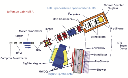
Figure 5: (Color online) Overhead view of the experimental setup for E06-014. The longitudinally polarized electron beam enters from the left and scatters from the longitudinally or transversely polarized ³He target, which is discussed in Section III. The Møller and Compton polarimeters provide beam polarization measurements, presented in Section II.4.2. The LHRS and BigBite spectrometers are positioned at 45^∘ with respect to the beamline and detect scattered electrons.

II.4 The Hall A beamline

The beamline in Hall A contains a number of important diagnostic components: BCMs, BPMs and the polarimetry apparatus. We first discuss the BCMs and BPMs in Section II.4.1, followed by the beam polarization measurements in Section II.4.2. The measurement of the beam energy is presented in Section II.4.3.

II.4.1 Beam charge and position monitoring

The experiment ran at beam currents of $\sim$15 $\mu$A. Fluctuations about the required value and beam trips, due to difficulties in the accelerator or in the other two experimental halls, make it important to monitor the beam current. To this purpose two BCMs, which are resonant RF cavities, are utilized. These cavities, stainless-steel cylinders with a $Q$-factor of $\sim 3000$, were tuned to the fundamental beam frequency of 1.497 GHz. The two BCMs were located 25 m upstream of the target, where one cavity was denoted as upstream and the other as downstream, based on their relative positions along the beamline. Each produced a voltage signal that was proportional to the measured current. Three copies of the signal were recorded, each amplified by a different gain factor (1, 3 or 10), resulting in six signals altogether (three for each cavity) Alcorn et al. (2004). Each copy of the signal was amplified by its assigned gain and then sent to a voltage-to-frequency converter. These signals were calibrated using a Faraday cup Parno (2011). Each signal was read out by scalers in the LHRS and BigBite spectrometers.

For accurate vertex reconstruction and proper momentum calculation for each detected electron, the position of the electron beam in the plane transverse to the nominal beam direction at the target was needed. The measurement of the beam position was accomplished through the use of two BPMs. They each consisted of four antenna arrays placed $\sim 7.5$ m and $\sim 1.3$ m upstream of the target. Pairs of wires were positioned at $\pm 45^{\circ}$ relative to the horizontal and vertical directions in the hall. The signal induced in the wires by the beam was inversely proportional to the distance from the beam to the wires, and was recorded by analog-to-digital converters (ADCs). The differences between the signals in pairs of wires in a given plane yields a positional resolution of 100 $\mu$m Allada (2010). Combining the measurements of the two BPMs yields the trajectory of the beam; extrapolating these data gives the position at the target. The BPMs were calibrated using wire scanners called harps. A single harp was located immediately downstream of each BPM. Harp measurements allow the relative position measurements from the BPMs to be tied to the Hall A coordinate system. They interfered with the beam, so dedicated runs called “bull’s eye” scans were needed. A “bull’s eye” scan consisted of five measurements with $(x,y)$ data points in the plane perpendicular to the beam momentum with the beam positioned at different locations. Four of these points described the corners of a 4 mm by 4 mm square, and the fifth data point measured the square’s center Parno (2011).

In order to avoid damage to the glass target cell due to beam heating, the beam was rastered (scanned) at high speeds (17–24 kHz) across a large rectangular cross section $\left(\approx 4\times 6\text{ mm}^{2}\right)$ at the target. This rectangular distribution was achieved by two dipole magnets (one for vertical, one for horizontal) located 23 m upstream of the target Alcorn et al. (2004).

II.4.2 Beam polarization measurement

The polarization of the electron beam was measured using two different polarimeters, a Møller and a Compton polarimeter. Møller polarimetry utilizes scattering the polarized electron beam from polarized atomic electrons in a magnetized iron foil. The scattering rate is proportional to the beam and foil polarizations Alcorn et al. (2004); Kresnin and Rozentsveig (1957); Glamazdin et al. (1999). Such a measurement required the insertion of a magnetized foil into the beam path which inhibited normal data-taking. A total of seven Møller measurements were made during the course of the experiment. This method has sub-percent statistical accuracy, but a sizable systematic uncertainty mainly due to uncertainty in the target foil polarization. The total relative systematic uncertainty on the Møller measurement during this experiment was $\sim 2$%.

The Compton polarimeter utilized $\vec{e}$-$\vec{\gamma}$ scattering to determine the polarization of the electron beam as the interaction is sensitive to the relative polarizations of the electrons and photons Lipps and Tolhoek (1954a, b). The newly commissioned polarimeter consisted of a magnetic chicane which deflected the electron beam towards a photon source and deflected unscattered electrons back towards the original beam path. At the center of the chicane was the photon source, a 700 mW laser at a wavelength of 1064 nm. The laser output was 400–500 W with a resonant Fabry-Pérot cavity Jorda et al. (1997). The laser polarization for the left- and right-circular polarization states was $99\%\pm 0.02\%$ during the experiment Parno (2011). There was also an electromagnetic calorimeter, a Gd₂SiO₅ (GSO) crystal doped with cerium, for detecting scattered photons Friend et al. (2012). The electron detector was not used in this experiment.

The electron polarization was extracted from an asymmetry in the rate of scattering circularly polarized photons from the longitudinally polarized electrons, between two unique spin configurations: electron and photon spins parallel and antiparallel. The energy-weighted, integrated asymmetry was measured in a new integrating DAQ and then combined with the polarimeter’s theoretically calculated analyzing power to determine the electron beam polarization Friend et al. (2012); Parno et al. (2013). Since Compton polarimetry is a non-invasive measurement, polarization measurements could be performed in parallel with data-taking.

Combining the results of the Møller and Compton measurements for the three production run periods with polarized beam resulted in a beam polarization of $74\%\pm 1\%$ ($E=5.89$ GeV), $79\%\pm 1\%$ ($E=5.89$ GeV) and $63\%\pm 1\%$ ($E=4.74$ GeV) Parno (2011).

II.4.3 Beam energy measurement

The beam energy was monitored throughout the experiment using the so-called Tiefenback method Tiefenback and Douglas (1992), which combined BPM measurements and the estimated integral of the magnetic field produced by the Hall A arc magnets. This method was calibrated against an invasive “Arc Energy” measurement. This measurement used the results of a detailed field mapping of all nine arc dipoles (including the reference one) after following a controlled excitation. In the actual Arc Energy measurement, all nine dipoles were excited following the same curve and the field was measured in the ninth dipole. The actual deflection of the beam was then measured and the beam energy was computed from the deviation from the nominal bend angle of 34.3^∘. The uncertainty on such a measurement was $\delta E/E\approx 2\times 10^{-4}$ Marchand (1998). Arc measurements were not performed during this experiment but were done for the immediately preceding experiment, E06-010 Qian et al. (2011). Their arc measurement was used as a reference for the Tiefenback measurements. The arc measurement conducted during E06-010 for $\sim 6$ GeV beam energies yielded a value of $5889.4\pm 0.5_{\text{stat}}\pm 1_{\text{syst}}$ MeV, while the Tiefenback measurement yielded $5891.3\pm 2.5_{\text{syst}}$ MeV Qian et al. (2011). In our data analysis we used the Tiefenback measurements without correcting for the difference relative to the arc measurement, which was $\ll 1\%$.

II.5 The spectrometers

II.5.1 The Left High-Resolution Spectrometer

The Hall A high-resolution spectrometers were designed for in-depth studies of the structure of nuclei and nucleons. The LHRS has high resolution in both the momentum and angle reconstruction of the scattered particles, in addition to the capability of running at high luminosity.

At the entrance of the LHRS there are two superconducting quadrupoles, for focusing the charged particles, followed by a superconducting dipole magnet that bends the charged particles upwards through a nominal $45^{\circ}$ bending angle. After this, the particles pass through a third quadrupole before entering the detector stack. The LHRS has an angular acceptance of 6 msr, for a horizontal (vertical) angular resolution of 0.5 mrad (1 mrad). The momentum acceptance is 10% with a momentum resolution of $10^{-4}$. The designed maximum central momentum is $4$ GeV Alcorn et al. (2004).

For E06-014 the LHRS detector stack was composed of a number of sub-packages, located in the shield hut at the end of the magnet configuration. The detector sub-packages included vertical drift chambers (VDCs), which provided tracking information for scattered particles, and the S1 and S2m scintillating planes served as the main trigger. Finally, the gas Čerenkov and the pion rejector yielded particle identification (PID) capabilities. The layout of the spectrometer is shown in Fig. 6.

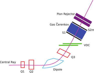
Figure 6: (Color online) The layout of the Left High-Resolution Spectrometer in Hall A of Jefferson Lab during E06-014. Drawing not to scale.

The VDCs allowed precise reconstruction of particle trajectories. Each chamber had two wire planes containing 368 sense wires, spaced 4.24 mm apart Alcorn et al. (2004); the wires were oriented orthogonally with respect to one another. The two wire planes lay in the horizontal plane of the laboratory, thus oriented at 45^∘ with respect to the central (scattered) particle trajectory. Gold-plated Mylar high-voltage planes were placed above and below each wire plane at an operating voltage of -$4$ kV, thus setting up an electric field between the high-voltage planes. This defined a “sense region” for each wire plane. The chambers were filled with a mixture of 62% argon and 38% ethane by weight. Traversing particles ionized the gas mixture; the ionization electrons drifted along the field lines to the closest sense wires, triggering a “hit” signal in the wires. A central track passing through at an angle of 45^∘ fired five sense wires on average, resulting in a positional resolution of $\sim 100$ $\mu$m and an angular resolution of $\sim 0.5$ mrad Alcorn et al. (2004).

The gas Čerenkov had ten spherical mirrors, each with a focal length of 80 cm, stacked in two columns of five. Each mirror was viewed by a photomultiplier tube (PMT), placed 45 cm from the mirror. The chamber was filled with CO₂ gas at STP with an index of refraction of 1.00043 Grupen and Shwartz (2008). This yielded a momentum threshold for triggering the gas Čerenkov of $\sim 17$ MeV for electrons and $\sim 4.8$ GeV for pions.

Incident particles were also identified using their energy deposits in the lead glass shower calorimeter, called a pion rejector. It was composed of two layers of thirty-four lead-glass blocks, the first 14.5 cm $\times$ 14.5 cm $\times$ 30 cm, the second 14.5 cm $\times$ 14.5 cm $\times$ 35 cm made of the material SF-5, which has a radiation length of 2.55 cm Bach and Neuroth (1995). The blocks were stacked so that the long dimensions of the blocks were transverse with respect to the direction of the scattered particle from the target. The gaps between the blocks in the first layer were compensated for by a slight offset in the second layer of blocks.

Since electrons and heavier particles like pions have different energy deposition distributions in electromagnetic calorimeters, we can distinguish between the two particle distributions, where electrons tend to leave most (if not all) of their energy in the calorimeter, while pions act like minimum ionizing particles (MIPs), leaving only a small amount of energy in the calorimeter. The energy loss of a MIP can be approximated by 1.5 MeV per g/cm${}^{\text{2}}$ traversed Green (2000). With the density of SF-5 being $\sim 4$ g/cm${}^{\text{3}}$ Grupen and Shwartz (2008), pions deposited $\sim 175$ MeV in the calorimeter (both layers of the pion rejector taken together). As a result there are two distinct peaks in the energy distribution with good separation in the calorimeter: one due to pions and the other due to electrons. This allows the selection of electrons in the analysis while rejecting pions.

Figure 7 shows a typical signal distribution in the gas Čerenkov. Electron (pion) candidates are indicated by the distributions centered at $\sim 6.5$ photo-electrons ($\lesssim 2$ photo-electron) in Fig. 7, that are obtained by placing cuts on the pion rejector signals. While scattered electrons yielded an ADC signal corresponding to the main photo-electron peak in the gas Čerenkov, pions may also influence the ADC spectrum. This occurs because pions could have ionized the atoms of the gaseous medium in the Čerenkov, producing electrons with enough energy to trigger the detector. Such electrons are called $\delta$-rays, or knock-on electrons. The distribution of these electrons has a peak at the one-photo-electron peak (leftmost peak in Fig. 7) with a long tail underneath the multiple (main) photo-electron peak. These knock-on electrons can effectively be removed in the analysis because on average they deposited less energy in the pion rejector. To identify electrons the ratio $E/p$ of the energy deposited in the pion rejector and the reconstructed momentum was required to be greater than 0.54, as illustrated in Fig. 8 (Section II.7). Additionally, events that deposited less than 200 MeV in the first layer of the pion rejector were removed from the analysis, as they were likely to be pions or knock-on electrons.

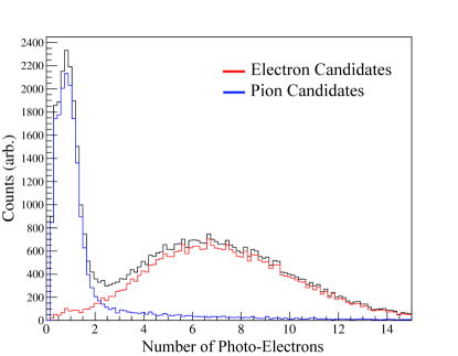
Figure 7: (Color online) A typical signal distribution in the LHRS gas Čerenkov (black curve). Electron (pion) candidates were selected by placing cuts on the energy deposited in the pion rejector, described by $E/p>0.54$ ($E/p<0.54$) and for the energy deposited in the first layer of the pion rejector to be greater than (less than) $200$ MeV. Electrons are indicated by the distribution centered at $\sim 6.5$ photo-electrons, while pion candidates have their distribution peaked at $\sim 1$ photo-electron.

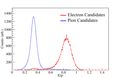
Figure 8: (Color online) A typical signal distribution in the LHRS pion rejector layers, where the particle’s total deposited energy divided by its reconstructed momentum is plotted. Electron (pion) candidates are shown by the distributions on the right (left), as selected by placing a cut on the gas Čerenkov signal to be greater than (less than) two photo-electrons.

There were two planes of plastic scintillating material, labeled S1 and S2m. S1 was composed of six horizontal scintillating paddles with 36 cm $\times$ 29.3 cm $\times$ 0.5 cm active area. Each paddle was viewed by a 5.1 cm-diameter photomultiplier tube (PMT) on each end. The paddles overlapped by 10 mm, oriented at a small angle with the S1 plane. The S2m plane consisted of sixteen non-overlapping paddles with dimensions of 43.2 cm $\times$ 14 cm $\times$ 5.1 cm. The timing resolution of the PMTs used for each plane was $\sim 50$ ps Qian (2010).

When a paddle absorbed ionizing radiation, it emitted light which traveled down the length of the paddle and is collected by the PMTs attached at each end. The timing information encoded in the PMTs’ TDCs is utilized in the formation of the LHRS main trigger, discussed in Section II.6.

II.5.2 The BigBite Spectrometer

The BigBite spectrometer is a large-acceptance spectrometer, able to detect particles over a wide range in scattering angle and momentum. BigBite consists of one large dipole magnet, capable of producing a maximum magnetic field of $\sim 1.2$ T. The magnet entrance was located 1.5 m from the target center, resulting in an angular acceptance of about 64 msr. Charged particles with momenta of $\sim 0.5$ GeV entering the magnet near its optical axis are then deflected roughly $25^{\circ}$ for a total trajectory of 64 cm when the field is 0.92 T de Lange et al. (1998). The momentum range covered by the spectrometer at full field had a lower bound of roughly 0.6 GeV. In its standard configuration, the magnet bent negatively charged particles upwards into the detector stack, while positively charged particles were deflected downwards. The large acceptance of the spectrometer allowed the detection of both negatively and positively charged particles. The detector stack for E06-014 included multi-wire drift chambers for particle tracking, a newly installed gas Čerenkov, a scintillator plane and an electromagnetic calorimeter, composed of a pre-shower and shower calorimeter. The gas Čerenkov, scintillator plane and the pre-shower and shower calorimeters were used for PID purposes. The schematic layout of BigBite is shown in Fig. 9.

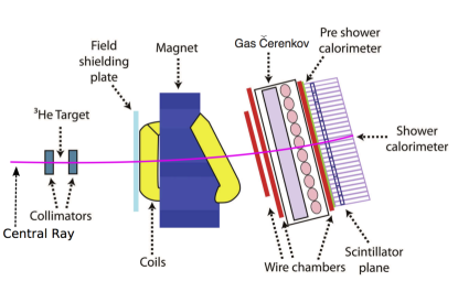
Figure 9: (Color online) The layout of the BigBite Spectrometer in Hall A of Jefferson Lab. Drawing not to scale. The central ray drawn here is a for a path similar to what a 1.7 GeV electron would take through the magnet. Figure modified from Qian (2010).

The Multi-Wire Drift Chambers (MWDCs) were utilized for particle tracking, in much the same way as described for the VDC planes in the LHRS. There were three chambers, each filled with a 50–50 mixture of argon and ethane gas. Each chamber had three pairs of wire planes, giving a total of eighteen planes in all. Each of the eighteen planes was perpendicular to the detector’s central ray (Fig. 9), bounded by cathode planes 6 mm apart from one another. Halfway between the cathode planes was a plane of wires, composed of alternating field and sense wires. The field wires and the cathode planes were held at the same constant high voltage, producing a nearly symmetric potential in the region close to the sense wires. Each pair of wire planes had a different orientation so as to optimize track reconstruction in three dimensions. The two so-called X-planes (X, X’) ran horizontally (in detector coordinates), while the U and V planes were oriented at $+30^{\circ}$ and $-30^{\circ}$ with respect to the X-planes, respectively. The wires in each plane were 1 cm apart and the primed planes (X’, U’, V’) were offset from their unprimed counterparts by 0.5 cm. This allowed the tracking algorithm to determine if the track passed above or below a given wire in the X plane based upon which wire registered a hit in the X’ plane, for example. This alignment resulted in a positional resolution of less than 300 $\mu$m Posik (2013).

The gas Čerenkov, which was constructed by Temple University specifically for this experiment Posik et al. , included twenty spherical mirrors, each with a focal length of 58 cm, stacked in two columns of ten. The chamber was filled with the gas C₄F₈O, which has an average index of refraction of 1.00135 Posik (2013). Čerenkov light incident on each mirror was reflected onto a corresponding secondary flat mirror. This mirror then directed the Čerenkov light onto the face of a corresponding PMT. To boost the amount of light collected, each PMT was fitted with a cone similar to a Winston cone Winston (1970). This extended the effective diameter of each PMT collection area from five inches to eight inches. The PMTs were recessed 5 ” within their shielding in order to reduce the effects of the BigBite magnetic field. The resulting gap between the PMT face and the edge of the shielding was filled with a cylindrical lining of Anomet UVS reflective material, so as to direct light incident upon this region onto the PMT face. Figure 10 shows a typical signal distribution in the gas Čerenkov. Electron (pion) events are indicated by the right (left) distributions. Electron events for a given PMT were identified by selecting those events that had a hit in their corresponding TDC with a projected track from the target that fell within the PMT’s geometrical acceptance.

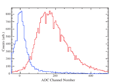
Figure 10: (Color online) Signal distributions in the BigBite gas Čerenkov. Electron (pion) events are shown by the right (left) distributions.

The calorimeter was composed of two layers of lead-glass blocks. The first layer was the pre-shower, composed of the material TF-5, which has a radiation length of 2.74 cm. The pre-shower was located 85 cm from the first drift chamber plane. It contained 54 blocks of dimensions 35 cm $\times$ 8.5 cm $\times$ 8.5 cm. They were organized in two columns of 27 rows. The long dimension of each block was oriented transverse with respect to scattered particles coming from the target. The shower layer was composed of the material TF-2, which has a radiation length of 3.67 cm and was located 15 cm behind the pre-shower and 1 m from the first drift chamber. It had 189 blocks of the same dimensions as the blocks in the pre-shower, but they were organized in seven columns and 27 rows. The long dimension of the block was oriented along the scattered particle path, ensuring the capture of a large amount of the electromagnetic shower of the particle .

The plane located between the pre-shower and the shower consisted of a scintillator plane composed of 13 paddles of plastic scintillator, each of which had a PMT at each end with a timing resolution of 0.3 ns. Each paddle had the dimensions 17 cm $\times$ 64 cm $\times$ 4 cm. The first dimension was transverse with respect to the scattered particles, while the short dimension was along the scattered particle path. This resulted in an active area of 221 cm $\times$ 64 cm. This plane provided an additional source of pion rejection to complement the gas Čerenkov and the shower calorimeter, as the charged pions left a significant signal in the low end of the ADC spectrum via knock-on electrons Posik (2013).

II.6 Data acquisition and data processing

In this experiment, the CEBAF Online Data Acquisition (CODA) III et al. (1994) system was used to process the various trigger signals and data coming from the LHRS and BigBite spectrometers, beamline and target equipment. The LHRS and the BigBite detector systems were run independently with a total of 5 TB of data recorded.

Eight triggers were configured for E06-014, summarized in Table 3. The T8 trigger was used for troubleshooting purposes only. It was a 1024 Hz clock, injected into the data stream to ensure that the electronics were working correctly. The T5 trigger was the coincidence (coin.) trigger between the LHRS and BigBite, used for optics calibration purposes.

Table 3: Triggers used during E06-014.

Trigger	Spectrometer(s)	Description
T1	BigBite	Low shower threshold
T2	BigBite	Coin. of T6 and T7
T3	LHRS	Coin. of S1 and S2m
T4	LHRS	Coin. of either S1 or S2m and Čerenkov
T5	LHRS, BigBite	Coin. of T1 and T3
T6	BigBite	High shower threshold
T7	BigBite	Gas Čerenkov
T8	LHRS, BigBite	1024 Hz Clock

The generation of the main LHRS trigger (T3) required a hit in both scintillating planes S1 and S2m, where a hit in a single plane corresponded to a signal in the two PMTs affixed to a paddle (left and right sides) in a plane. Thus, a T3 trigger corresponded to a pulse detected in four PMTs, two in the S1 plane and two in the S2m plane. The timing of this trigger was set by the leading edge of the TDC signal recorded in the PMT attached to the right side of the S2m scintillator paddles Allada (2010). The second LHRS trigger was the T4 trigger. The only difference between the T3 and T4 triggers was that a T4 was generated when there was a coincidence between either S1 or S2m and the gas Čerenkov detector, without generating a T3 trigger. The T4 trigger was used to study the efficiency of the T3 trigger, as these events were potentially good events since they generated a signal in the gas Čerenkov. It was found that the efficiency of the T3 trigger was $99.95\%$ over the course of the experiment Flay (2014).

The BigBite spectrometer had four dedicated triggers, T1, T2, T6, and T7. The T1 and T6 triggers involved taking the hardware (voltage) sum of the calorimeter blocks belonging to the cluster with the largest signal, where a cluster for the pre-shower and shower calorimeters was defined as two adjacent rows of calorimeter blocks. There are 26 clusters each for the pre-shower and shower calorimeters. The sum of the pre-shower and shower signals was then formed and sent to a discriminator. If this signal was greater than $\sim 300$–$400$ MeV ($\sim 500$–$600$ MeV), then the T1 (T6) trigger was formed. The T7 trigger was formed in a manner similar to the T1 and T6 triggers, but using the Čerenkov detector instead of the pre-shower or shower calorimeter. The Čerenkov signals from two adjacent rows of mirrors (four mirrors in total) were summed, resulting in nine overlapping mirror clusters. If this sum was larger than the set threshold value ($>1$–$1.5$ photo-electrons), then the T7 trigger was formed. The main trigger for the BigBite spectrometer, T2, imposed a geometric constraint on the incident particle track by requiring a coincidence between the geometrically overlapping regions in the gas Čerenkov and the calorimeter. An example of an event that generated a T2 trigger is illustrated in Fig. 11: a particle that triggered cluster C1 in the gas Čerenkov would also have to trigger at least one of the clusters A–D in the calorimeter. Similar coincidences were imposed for the eight other groupings that could form a T2 trigger.

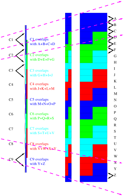
Figure 11: (Color online) The geometrical overlap for the main trigger for the BigBite spectrometer. The Čerenkov mirrors are represented by the leftmost column, where the cluster groupings are labeled by C$i$, with $i=1,\ldots,9$. The pre-shower blocks are shown as the middle column of colored blocks, while the shower blocks are the long blocks in the rightmost column. The calorimeter cluster groupings are labeled with the letters A–Z. The dashed lines indicate typical electron paths at the extremes of the acceptance of the BigBite spectrometer.

The raw data were processed by the Hall A Analyzer Ana , which is based on ROOT ROO . Specific C++ classes have been written to interpret the data recorded by the various detectors and their sub-detectors. For instance, there are classes that convert the ADC signals registered in a calorimeter block into the corresponding amount of energy deposited. There are also classes that handle the computation of a particle’s path (or track) through the LHRS (and BigBite) up to its focal plane and its reconstructed vertex position back at the target. The optics for BigBite required special attention, as discussed in Qian (2010); Posik (2013); Parno (2011).

II.7 Particle identification

The LHRS and the BigBite spectrometers each utilized a gas Čerenkov detector and a double-layered lead-glass shower calorimeter for PID purposes. In this experiment, PID corresponds to distinguishing electrons from pions, that constituted the primary background.

The PID performance of each detector was characterized by the efficiencies of the conditions (or cuts) placed on the corresponding observable. Before PID cut efficiencies were evaluated, the sample distribution of events to be studied was selected using data quality criteria (such as removing beam trips) and conditions to remove events that may have originated in the target’s glass endcaps Flay (2014); Posik (2013). The electron cut efficiency $\varepsilon_{e}$ is defined as the ratio of the number of events that pass a given cut to the size of the electron event sample defined by another detector. For the gas Čerenkov, the electron sample was chosen by using the calorimeter, and vice-versa. To characterize how well a given detector can reject pions, the rejection factor $f_{\pi,\text{rej}}$ is evaluated. It is defined as the ratio of the size of the selected pion sample to the number of events misidentified as electrons for a given cut. The PID cuts were chosen such that the pion rejection was maximized while the highest electron efficiency was maintained.

In the momentum acceptance range of the experiment, $0.6$ GeV $\leq p\leq 1.7$ GeV, the electron cut efficiency for the LHRS gas Čerenkov was found to be $\varepsilon_{e}^{\text{cer}}\approx$ 96% for a cut of greater than two photoelectrons in the ADC. For the LHRS pion rejector, $\varepsilon_{e}^{\text{pr}}\approx$ 99% for $E/p>0.54$. These efficiencies are critical for the LHRS data since they contribute directly in the determination of the unpolarized cross section (Section IV.2). The pion rejection factor was found to be $\sim 660$ for both the gas Čerenkov and pion rejector, resulting in a combined rejection of $f_{\pi,\text{rej}}\approx 4\times 10^{5}$ Flay (2014). As a result, the pion contamination in the final electron sample was negligible.

PID studies were also conducted for the data recorded by BigBite. Here, the pion rejection factor was determined to be better than $2\times 10^{4}$ when combining the pion rejection capabilities of the gas Čerenkov , pre-shower and shower calorimeters, and the scintillator plane Posik (2013). Unlike the cross section analysis using the LHRS data, the electron cut efficiencies do not play a role in the asymmetry extraction that is performed using the BigBite data; the efficiencies cancel in the asymmetry defintion (Section IV.3).

III Polarized ³He target

Since the lifetime of the neutron is less than 15 minutes Wietfeldt (2014) outside the nucleus, a free-neutron target is not practical. ³He, a spin-1/2 nucleus consisting of two protons and a neutron, is a candidate for a polarized neutron target. Deuterium, a spin-1 nucleus consisting of a proton and a neutron, is another option. Both nucleons in deuterium have their spins aligned with the nuclear spin. However, large corrections due to the proton result in large uncertainties when using a deuterium target. When ³He is polarized, there are three principal states in play: $\sim 90$% of the time the nucleus is in the symmetric $S$ state; $\sim 1.5$% of the time the nucleus is in the $S^{\prime}$ state, and $\sim 8$% of the time the nucleus is in the $D$ state, see Fig. 12. In the $S$ state, the spins of the protons are antiparallel to one another, resulting in the neutron carrying the majority of the ³He polarization Friar et al. (1990). As a result, a polarized ³He target can be used as an effective polarized neutron target.

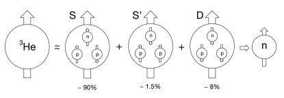
Figure 12: ³He ground states. The dominant state is the $S$ state, where $\sim 90$% of the polarization is carried by the neutron. In this state, the protons pair to $s=0$.

In this experiment, polarized ³He $\left({}^{3}\vec{\text{He}}\right)$ was used to study the electromagnetic structure and the spin structure of the neutron. Two major methods exist to polarize ³He nuclei. The first one uses the metastable-exchange optical pumping technique Colegrove et al. (1963), while the second method utilizes both spin-exchange Happer (1972); *Appelt and optical pumping Chupp et al. (1987), dubbed hybrid spin-exchange optical pumping.

³⁹K atoms were optically pumped using 795-nm circularly polarized laser light, inducing the D1 transition in ⁸⁵Rb: $5^{2}S_{1/2}$ ($m=-1/2$) $\rightarrow 5^{2}P_{1/2}$ ($m=+1/2$), in accordance with the selection rule of $\Delta L=+1$. The excited ⁸⁵Rb electrons decay from the $p$ orbital to the $s$ orbital with equal probabilities for the $m=\pm 1/2$ sub-states, but the excitation only occurs for the $m=-1/2$ initial state of the $s$ orbital; this results in the selective population of the $m=1/2$ state of the $s$ orbital. Second, the polarization of the ⁸⁵Rb atoms was transferred to the ³⁹K atoms via spin-exchange binary collisions Happer (1972). In the third and final step, the polarization of the ⁸⁵Rb and ³⁹K atomic electrons was transferred to the ³He nuclei via the hyperfine interaction, where the nuclear spin of ³He takes part in the process Walker and Happer (1997); *Newbury. The use of ³⁹K greatly decreases the spin-relaxation rate for collisions involving ³He, resulting in an increase in the spin-exchange efficiency of the polarization process Walker et al. (1997).

As the atomic electrons decayed to the ground state, photons were emitted. These photons were typically unpolarized, and therefore reduced the efficiency of the pumping process. To minimize this effect for the alkali atoms, a small amount of N₂ buffer gas was added to the cell. The excitation energy of the alkali atoms was passed to the rotational and vibrational modes of the buffer gas via collisions, reducing the emission of photons Appelt et al. (1998).

III.1 Setup

The target apparatus was composed of a number of different elements: the target cells, target oven, target ladder system, Helmholtz coils for the holding magnetic field, RF coils and polarizing lasers. The layout of the target system is shown in Fig. 13. The outer circle and large straight lines intersecting at right angles inscribed in the large circle represent Helmholtz coils. The smaller vertical straight lines and circle overlapping with the Helmholtz coils signify the RF coils. Pickup coils mounted near the target cell are also shown.

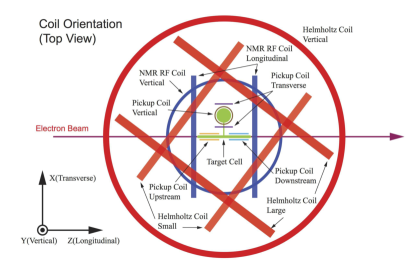
Figure 13: (Color online) The target setup. The Helmholtz coils for the holding magnetic field and coils for the RF field are shown. The pickup coils near the target cell are used for NMR measurements. Figure reproduced from Alcorn et al. (2004).

Two pairs of Helmholtz coils, capable of producing magnetic fields in two orthogonal directions, were utilized in E06-014: longitudinal (along the direction of the beam), and transverse in-plane (perpendicular and horizontal to the beam). The field reached a magnitude of 25 G, requiring $\sim 7$ A of current in each coil. The RF coils and pickup coils are important for the measurement of the target polarization, as presented in Sections III.4 and III.5.

III.2 Target cells

The production target cell, named Samantha, is shown schematically in Fig. 14. The upper chamber, called the pumping chamber, contained ³He, alkali metals (⁸⁵Rb and ³⁹K at equal densities) and N₂, with number densities of $10^{20}$ cm^-3, $10^{14}$ cm^-3 and $10^{18}$ cm^-3, respectively Dutta (2010). This chamber was heated to $\sim 265^{\circ}$C in order to keep the Rb and K in a gaseous state. The polarization process took place in this chamber. The polarized ³He gas (with the N₂ mixture) flowed through a thin transfer tube to the target chamber, thanks to the temperature gradient between the pumping chamber and the target cell that was kept at room temperature. This chamber was 40 cm long and contained $\sim 8$ atm of ³He and $\sim 0.13$ atm of N₂ during the experiment. The temperature of the cell was monitored via resistive temperature devices (RTDs), which were placed equidistant from one another along the length of the target chamber, along with two more placed on the pumping chamber; one at the top and the other at the base. The production cell was made out of aluminoscilicate glass (GE-180), which was filled and characterized at the University of Virgina and the College of William and Mary Allada (2010). This characterization consisted of measuring the polarization, gas density, glass thickness of the cell and rate of polarization.

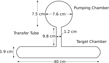
Figure 14: The production target cell used in our experiment. The top spherical chamber is the pumping chamber where the polarization of ³He takes place. The long cylindrical chamber is the target cell, through which the electron beam passes longitudinally. The thin tube connecting these two chambers is the transfer tube, which allows polarized ³He to drift down into the target chamber. Drawing not to scale.

An additional reference cell was used , which could be filled with H₂, N₂ or ³He. This allowed the determination of the dilution factors that contribute to the cross sections and asymmetries. RTDs were also mounted on the reference cell to monitor its temperature, in a similar configuration as was done for the target cell. A multi-carbon foil (“optics”) target—as well as the reference cell filled with hydrogen gas—was used for the calibration of the optics for the two spectrometers. All of these targets were mounted on a target ladder, which could be moved vertically up and down to select the target needed. In addition to these targets, a “no target” position was available, corresponding to a hole in the target ladder. It was used during Møller polarimeter measurements, so that the target assembly would not be damaged in the process.

III.3 Laser system

Our experiment utilized an upgraded laser system that had been installed for the immediately preceding experiment, E06-010 Qian et al. (2011). These new COMET lasers had a linewidth of 0.2 nm, a factor of ten less than that of their predecessors (FAP lasers Zheng (2002); Kolarkar (2008); Kelleher (2010)). This dramatically improved the optical pumping efficiency, since a narrower linewidth results in proportionately more photons exciting the desired atomic transitions in ⁸⁵Rb, so that a higher polarization of ³He atoms could be attained in a shorter timeframe Dutta (2010).

The laser setup is shown in Fig. 15. It consisted of three COMET lasers, each with a power of 25 W and a wavelength of 795 nm, used to optically pump the ⁸⁵Rb in the pumping chamber. The lasers were installed in a separate laser building behind the counting house on the accelerator site at JLab. The fiber coming out of each COMET control unit was connected to a 75-m-long fiber that ran from the laser building to the hall. Then the fiber was connected to a 5-to-1 combiner. The output of the combiner was sent to a beamsplitter, yielding two linearly polarized components. One component passed twice through a quarter-wave plate, after which both had the same linear polarization. Sending each component through another quarter wave plate converted the linear polarization into circular polarization. The resulting beams were then combined into one, with a spot size of 7.5 cm in diameter, the size of the pumping chamber Dutta (2010). There were three optics lines corresponding to the longitudinal, transverse and vertical polarization directions. The polarizing optics were set up in an antiparallel pumping configuration such that the target spin was always oriented opposite to the magnetic holding field Posik (2013).

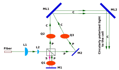
Figure 15: (Color online) The laser system used to polarize ⁸⁵Rb atoms. The symbols labeled L1 and L2 are lenses, while symbols labeled as M and ML are mirrors. Light reflected from ML2 is incident upon another mirror (not shown) which is attached to the oven. Quarter wave plates are indicated by Q1, Q2 and Q3. The beam-splitting polarization cube (BSPC) is represented by the rectangle with a slash through it. The initial unpolarized laser light is split by the BSPC into S- and P-wave components, where the P-wave component has linear polarization and passes through the beam splitter. The S-wave component is converted into a P-wave by Q1. The motorized quarter-wave plates Q2 and Q3 convert P-wave light into circularly polarized light, labeled C. Figure reproduced from Posik (2013).

III.4 EPR measurements

The target polarization was measured in an absolute sense through an electron paramagnetic resonance (EPR) measurement, that utilized Zeeman splitting of the electron energy levels when an atom was placed in an external magnetic field. This phenomenon occurred for the ⁸⁵Rb and ³⁹K atoms, which were present in the pumping chamber. The ground states of the alkali metals split into $2F+1$ energy levels, where $F$ is the total angular momentum quantum number. Specifically, for ⁸⁵Rb, the $F=$ 3 ground state split into seven sublevels corresponding to $m_{F}=-3$,…, $3$. For ³⁹K, the $F=2$ ground state split into five energy levels, given by $m_{F}=-2$,…, $2$. The splitting corresponded to a frequency that is proportional to the holding field. This frequency was shifted due to the small effective magnetic field created by the spin-exchange mechanism of ⁸⁵Rb–³⁹K and ³⁹K–³He, in addition to the polarization of the ³He nuclei.

When the EPR transition was excited, an alkali metal (either Rb or K as chosen by the excitation frequency) lost its polarization. When one of the metals was depolarized, so was the other due to the fast spin-exchange mechanism. Upon re-polarization of the Rb atoms, there was an increase in the photons emitted corresponding to the $P_{1/2}\rightarrow S_{1/2}$ (D1) transition (795 nm). However, due to thermal mixing between the $P_{1/2}$ and $P_{3/2}$ energy states and occasional collisional mixing with N₂ in the cell, the $P_{3/2}\rightarrow S_{1/2}$ (D2) transition (780 nm) was possible. While the amount of D1 and D2 flourescence was roughly the same Dutta (2010), the D1 light was suppressed due to a large background component corresponding to the polarizing laser light. Therefore, a filter was attached to a photodiode to identify the D2 light. During the measurement, the RF was modulated with a 100 Hz sine wave, and the D2 transition was synchronized to this modulating signal and measured by a lock-in amplifier. The signal from the lock-in output was proportional to the derivative of the EPR fluorescence curve as a function of the RF; the EPR resonance occured when the derivative was equal to zero Huang (2012); Dutta (2010). EPR measurements were performed every few days.

To determine the polarization in the target chamber, a model Romalis (1997); Singh et al. ; Ye et al. (2010); Dolph et al. (2011) was used to describe the diffusion of the ³He polarization from the pumping chamber to the target chamber. The relative systematic error of the measurement was $\sim 4\%$, dominated by the uncertainties on the dimensionless constant $\kappa_{0}$ Kadlecek et al. (2005) and the number density of the gas in the pumping chamber Posik (2013).

III.5 NMR measurements

Another method we used for measuring the polarization of the ³He nuclei was measuring the ³He nuclear magnetic resonance signal. The magnetic moments of ³He nuclei aligned along the direction of an external magnetic holding field had their direction reversed by applying an RF field in the perpendicular direction. Sweeping the frequency of the RF field through the resonance of the ³He nucleus flipped the spins of the nuclei. This spin flip changed the field flux through the pick-up coils (Fig. 13), inducing an electromotive force. The signals from the coils were pre-amplified and combined, and sent to a lock-in amplifier. The magnitude of the final signal was proportional to the ³He polarization.

The RF is swept according to the Adiabatic Fast Passage (AFP) technique Abragam (1961), in which the sweep through the resonant frequency is done faster than the spin-relaxation time, but slowly enough so that the nuclear spins can follow the sweep of the RF field. This minimizes the effect of these NMR measurements on the target polarization.

An NMR measurement is a relative measurement, so it needs to be compared against a known reference. A measurement of NMR on water is typically used, for which the polarization can be calculated exactly from statistical mechanics Lorenzon et al. (1993). However, in E06-014, water-cell measurements were available only for the longitudinal target polarization configuration, as conversion factors needed to account for the different positions of the water and ³He cells could not be measured for the transverse configuration Posik (2013). Because of this, the NMR measurements were calibrated against EPR measurements (Section III.4) that were done close in time relative to the NMR measurements. The NMR water measurements in the longitudinal configuration were used as a cross-check against the EPR measurements, and were found to be consistent to the 1% level. NMR measurements were performed every four hours on the production ³He target. The systematic error on the NMR measurement was $\sim 3.9\%$ (relative), dominated by the uncertainties on the EPR calibration and on the computed magnetic flux through the pickup coils Posik (2013).

III.6 Target performance

The target polarization over the course of the experiment, extracted from NMR measurements, is shown in Fig. 16. In the data analysis (Section IV.3), the target polarization data was utilized on a run-by-run basis. On average, the target polarization achieved was 50.5% with a relative uncertainty of 7.2% (3.6% absolute). The dominant contribution to the uncertainty was from the calibration of the NMR measurements against the EPR measurements (3.9% relative) and the loss of polarization due to the diffusion of polarized ³He from the pumping chamber to the target chamber (6% relative).

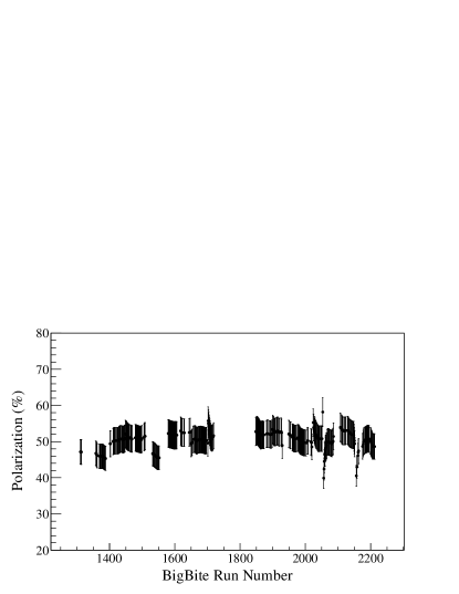
Figure 16: The ³He target polarization as a function of BigBite run number.

IV Data Analysis

IV.1 Analysis procedure

The analysis procedure is outlined in Fig. 17, which shows that the raw data were first replayed, followed by the calibration and data quality checks. Data calibrations included gain-matching ADC readings within the gas Čerenkov and shower calorimeters to have the same responses for a given type of signal. Calibrations also involved optimizing the software packages that describes the optics of the two spectrometers. Multi-foil carbon targets, a sieve slit collimator and elastic ¹H$(e,e^{\prime})p$ data at an incident energy of $E=1.23$ GeV were used to calibrate the optics software package for the LHRS Qian et al. (2011) and for the BigBite spectrometer. The momentum resolution achieved for the BigBite spectrometer was $\sim 1\%$ Posik (2013). Data quality checks implied checking the calibration results and removing beam trips from the data. Faulty runs (e.g., those having poor beam quality, detector live-times $\lesssim 80\%$, run times less than a few minutes, etc.) were also identified and discarded from the analysis.

Following calibration and data quality checks, the electron sample was cleaned up by removing events that did not generate a good trigger or had poor track reconstruction. Cuts were also made to remove pion tracks and events originating in the target window. In the BigBite data set, geometrical cuts had to be implemented to remove events that rescattered from the BigBite magnet pole pieces. After all cuts had been applied to the data, the raw physics observables consisting of cross sections and asymmetries were then extracted. Corrections were applied to account for the nitrogen target contamination and background due to pair-produced electrons, neither of which could be removed by cuts. After these corrections were applied, we obtained the experimental cross sections (Section IV.2) and the experimental asymmetries (Section IV.3). Applying radiative corrections yielded the final quantities for each of those, from which the spin structure functions $g_{1}$ and $g_{2}$ on ³He were extracted as described in Appendix A.6. The ³He results for the unpolarized cross sections, double-spin asymmetries and spin structure functions $g_{1}$ and $g_{2}$ are presented in Section V.1. The Lorentz color force $d_{2}^{{}^{3}\text{He}}$ was obtained from Eq. I.2, after which nuclear corrections (Section IV.4) were applied to obtain $d_{2}^{n}$ (Section V.2.1). From the $g_{1}^{{}^{3}\text{He}}$ data the $a_{2}$ matrix element on ³He (given as the third moment of $g_{1}$) was extracted. Nuclear corrections, similar to those used for $d_{2}$, were applied to obtain $a_{2}^{n}$ (Section V.2.2). From a twist expansion of world data for $\Gamma_{1}^{n}$, the twist-4 matrix element $f_{2}^{n}$ was obtained using our $d_{2}^{n}$ data as input (while the value of $a_{2}^{n}$ was taken from an average over the available model calculations, see Section V.2.3). Additionally, $A_{1}^{{}^{3}\text{He}}$ and $g_{1}^{{}^{3}\text{He}}/F_{1}^{{}^{3}\text{He}}$ were extracted with the aid of Eqs. 18 and 19. Nuclear corrections were then applied to the ³He results to obtain the neutron quantities (Sections V.2.4 and V.2.5). Using the $g_{1}^{n}/F_{1}^{n}$ data obtained, we then extracted the flavor-separated ratios $(\Delta u+\Delta\bar{u})/(u+\bar{u})$ and $(\Delta d+\Delta\bar{d})/(d+\bar{d})$ (Section V.3).

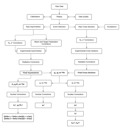
Figure 17: The data analysis procedure.

IV.2 Cross sections

IV.2.1 Extraction of raw cross sections from data

The unpolarized differential cross section was calculated from the data for a given run as follows:

$$\frac{d^{3}\sigma_{\text{raw}}}{d\Omega dE^{\prime}}=\frac{t_{ps}N_{\text{cut}}}{(Q/e)nt_{LT}\varepsilon}\frac{1}{\Delta E^{\prime}\Delta\Omega\Delta Z},$$ (28)

where $t_{ps}$ denotes the prescale value for the T3 trigger , $N_{\text{cut}}$ the number of electrons that pass all cuts, $Q/e$ the number of beam electrons delivered to the target, $n$ the target number density in amagats , $t_{LT}$ the live-time , and $\varepsilon$ the product of all detector (cut) efficiencies. The quantity $\Delta E^{\prime}=\delta p/p_{0}\cdot p_{0}$, where $\delta p/p_{0}=(p-p_{0})/p_{0}$ is the scattered momentum of the electron $p$ relative to the LHRS momentum setting $p_{0}$. Electrons were selected according to the criterion $\left|\delta p/p_{0}\right|<3.5$%, which was based on the agreement of the Monte Carlo simulation of the spectrometer (see below) with the data Flay (2014). The quantity $\Delta Z$ denotes the effective target length seen by the spectrometer, measured in meters. The cut on the effective target length was chosen such that the target windows and edge effects due to scattering from the magnets in the LHRS are removed. The term $\Delta\Omega$ denotes the solid-angle acceptance, measured in steradians; it is defined as the product of the in-plane scattering angle $\Delta\theta$ and out-of-plane scattering angle $\Delta\phi$. The cut chosen for $\Delta\theta$ ($\Delta\phi$) was $\pm 40$ mrad ($\pm 20$ mrad), which amounts to a solid angle of 3.2 msr. The cuts on $\delta p/p_{0}$, $\Delta Z$, $\Delta\theta$ and $\Delta\phi$ were informed by looking at a Monte Carlo simulation of the LHRS.

The effective acceptance was determined with the Single-Arm Monte Carlo (SAMC) simulation SAM . To determine how the geometrical acceptance of the LHRS deviates from the ideal rectangular acceptance, SAMC began by generating events originating from the target that were uniformly distributed over the kinematical phase space. Each event was then transported to the focal plane using an optical model of the LHRS LeRose . As the particle encountered each magnet aperture in the LHRS, a check was performed to see if it successfully passed through the known apertures. If the simulated particle successfully made it through all geometrical apertures, it was then reconstructed back to the target using the optics matrix optimized during the experiment. The ratio $r$ of the number of reconstructed events to the number of generated events was used to determine the effective acceptance, written as $r=\Delta E^{\prime}\Delta\Omega\Delta Z/\Delta E^{\prime}_{\text{MC}}\Delta\Omega_{\text{MC}}\Delta Z_{\text{MC}}$. The subscript MC refers to the initially generated kinematic phase space in the simulation, chosen to be larger than the apertures of the LHRS, so as to avoid edge effects.

The cross sections extracted for each run of a given momentum bin were then averaged, weighted by their statistical errors:

$$\langle\sigma\rangle=\frac{\sum\limits_{i=0}^{n}\sigma_{i}\frac{1}{\delta\sigma_{i}^{2}}}{\sum\limits_{i=0}^{n}\frac{1}{\delta\sigma_{i}^{2}}},$$ (29)

where $\delta\sigma_{i}$ is the statistical error on the cross section for the $i^{\text{th}}$ run.

IV.2.2 Background corrections

The raw ³He cross section measured in the LHRS, $\sigma_{\text{raw}}$, contains contributions from electrons that were not scattered from ³He, but were produced in processes corresponding to electron-positron (pair) production (arising from $\pi^{0}$ mesons decaying predominantly to photons), or scattering from nitrogen nuclei.

To remove the pair-production contributions from $\sigma_{\text{raw}}$, several runs were taken with the LHRS in positive polarity mode (i.e., detecting positrons) to measure the positron cross section, $\sigma^{e^{+}}$. The nitrogen electron cross section $\sigma_{\text{N}_{2}}^{e^{-}}$ was measured by filling the additional reference target cell (Section III.2) with nitrogen gas and exposing it to the beam. Pair production also occurs when scattering from nitrogen nuclei, so a nitrogen positron cross section, $\sigma_{\text{N}_{2}}^{e^{+}}$, was also measured with the LHRS in positive polarity mode. The positron cross section on nitrogen $\sigma_{\text{N}_{2}}^{e^{+}}$ was subtracted from $\sigma_{\text{N}_{2}}^{e^{-}}$ to avoid double-counting the pair-produced events in the measurement that were already accounted for in $\sigma^{e^{+}}$. In principle, one has to consider pion background contributions; however, given the high pion suppression in the LHRS (Section II.7), this component was found to be negligible. Combining the measurements for $\sigma_{\text{raw}}$, $\sigma^{e^{+}}$, $\sigma_{\text{N}_{2}}^{e^{-}}$, $\sigma_{\text{N}_{2}}^{e^{+}}$, yielded the experimental ³He cross section, $\sigma_{\text{exp}}$:

$$\sigma_{\text{exp}} = \sigma_{\text{raw}}-\sigma^{e^{+}}-\sigma_{\text{N}_{2}}^{\text{dil}}$$ (30)

$$\sigma_{\text{N}_{2}}^{\text{dil}} = \frac{n_{\text{N}_{2}}}{n_{\text{N}_{2}}+n_{{}^{3}\text{He}}}\left(\sigma_{\text{N}_{2}}^{e^{-}}-\sigma_{\text{N}_{2}}^{e^{+}}\right),$$ (31)

where $n_{\text{N}_{2}}$ is the number density of nitrogen in the production cell and $n_{{}^{3}\text{He}}$ is the number density of ³He in the production cell.

When the nitrogen reference cell was in the beam, the number density for the cell was extracted using the measured temperature and pressure of the cell. This number density was used when extracting a nitrogen cross section (Eq. 28). A systematic uncertainty of 2.2% was estimated by computing the number densities while varying the temperature and pressure by up to 2^∘ C and 2 psig, respectively Posik (2013). In the ³He production cell, the number density of nitrogen $n_{\text{N}_{2}}$ was taken to be 0.113 amg (Eq. 31). This value was recorded as the target was initially filled, and is accurate to 3% from a pressure curve analysis.

Due to time constraints and hardware problems encountered during the experiment, there were not enough data to map out the background contributions to the raw cross section for all kinematic bins. To resolve this issue, empirical fits to the positron and nitrogen data (see Appendix C.1) were used to subtract those contributions. Figures 18 and 19 show the raw electron cross section, the positron and nitrogen cross sections (scaled by the ratio of the nitrogen number density to that of ³He in the production target cell), and the background-subtracted electron cross section, $\sigma_{\text{exp}}$. The error bars on the data points represent the statistical uncertainties. The largest correction was due to the positrons, at $\sim 53$% in the lowest $x$ bin, and fell to a few percent for $x\gtrsim 0.5$.

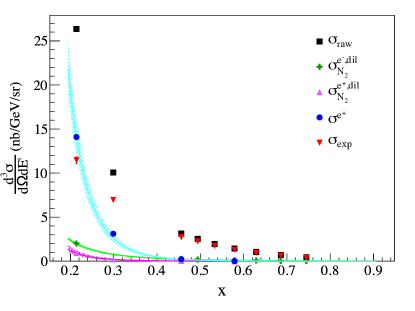
Figure 18: (Color online) Cross sections as a function of Bjorken-x at $E=4.74$ GeV. The squares show the raw electron cross section, and the circles (and fit) show the positron cross section measured on the ³He target. The cross data (and fit) represent the diluted nitrogen cross section measured on the N₂ target, and the up-triangle data (and fit) show the diluted nitrogen cross section measured in positive polarity mode on the N₂ target. The down-triangle data points are the final background-subtracted data, $\sigma_{\text{exp}}$. The error bars on the data points represent the statistical uncertainties.

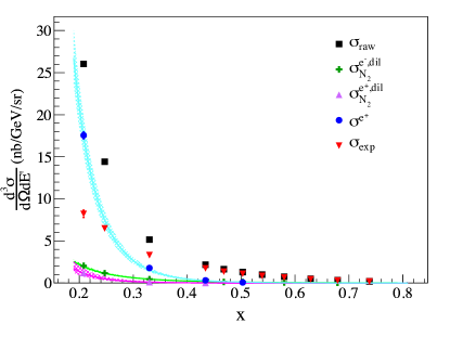
Figure 19: (Color online) Cross sections as a function of Bjorken-x at $E=5.89$ GeV. The description of the various data sets is the same as in Fig. 18.

IV.2.3 Radiative corrections

A first correction that must be done before carrying out the radiative corrections is to subtract the elastic and quasi-elastic radiative tails, since they are long and affect all states of higher invariant mass $W$ Mo and Tsai (1969). For these kinematics, the elastic tail was small and affects the lowest bins in scattered electron energy $E^{\prime}$ at the $\lesssim$ 1% level only. The elastic tail was computed following the exact formalism given by Mo and Tsai Mo and Tsai (1969), and using elastic ³He form factors from Amroun Amroun et al. (1994). The ³He quasi-elastic tail, however, was much larger, at $\sim 25$–$30\%$ in the lowest $x$ bin. The quasi-elastic radiative tail was computed by utilizing an appropriate model of the ³He quasi-elastic cross section Lightbody and O’Connell (1988) and applying radiative effects Stein et al. (1975). The tail was then subtracted from the data. The model was checked against existing quasi-elastic ³He data Day et al. (1979); Marchand et al. (1985); Meziani et al. (1992) covering a broad range of kinematics.

After the elastic and quasi-elastic tails had been subtracted from the data, radiative corrections were applied according to Mo and Tsai (1969); Tsai (1971), where the internal corrections were calculated using the equivalent radiator method and the external corrections were performed using the energy peaking approximation. In the experiment, we took production data for only two beam energies of 4.74 GeV and 5.89 GeV. However, we needed enough data to properly calculate the integrals involved in the radiative correction procedure. Therefore, we used the F1F209 cross section parameterization Bosted and Mamyan (2012) to fill in the rest of the phase space for each data set. The radiative corrections were as large as $\sim 50\%$ in the lowest measured $x$ bin, and fell off to a few percent at the large $x$ bins.

The resulting final ³He cross sections for E = 4.74 GeV and 5.89 GeV are presented in Fig. 20. The data are tabulated in Tables 4 and 5. The uncertainty on the final cross section arising from the radiative corrections was determined by varying the contributions to the radiative correction calculations, including the radiation thicknesses in the incident and scattered electron path, and considering different models for the elastic and quasi-elastic tail calculations. Of these, the quasi-elastic tail gave the biggest uncertainty, $\sim$ 5–6% for the lowest $x$ bin, falling to $\sim 1\%$ for all other bins. A full breakdown of the uncertainties on the final results is given in Tables 23 and 24 in Appendix E.1.

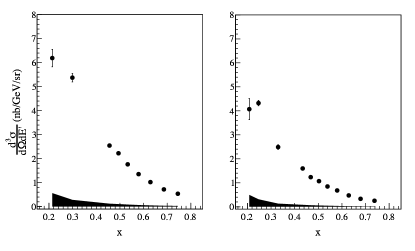
Figure 20: The final ³He unpolarized cross sections as a function of Bjorken-$x$. The left (right) panel shows $E=4.74$ GeV (5.89 GeV) data. The error bars show the statistical uncertainty, while the bands represent the systematic uncertainty.

IV.3 Asymmetries

IV.3.1 Extraction of raw asymmetries from data

The raw double-spin asymmetries were extracted from the data recorded in the BigBite detectors according to:

$$A_{\parallel}^{\text{raw}} = \frac{N^{\downarrow\Uparrow}-N^{\uparrow\Uparrow}}{N^{\downarrow\Uparrow}+N^{\uparrow\Uparrow}}$$ (32)

$$A_{\perp}^{\text{raw}} = \frac{1}{\langle\cos\phi\rangle}\frac{N^{\downarrow\Rightarrow}-N^{\uparrow\Rightarrow}}{N^{\downarrow\Rightarrow}+N^{\uparrow\Rightarrow}},$$ (33)

where $N$ denotes the number of electron counts after applying data quality and PID cuts for a particular beam and target spin configuration, $\downarrow$ ($\uparrow$) corresponds to the electron’s spin polarized antiparallel (parallel) to its momentum, $\Uparrow$ indicates that the target was polarized parallel to the electron momentum, and $\Rightarrow$ indicates that the target was polarized transverse to the electron momentum.

In E06-014, there were three target-spin configurations, either parallel ($\parallel$, referred to here as longitudinal) or transverse ($\perp$, in two orientations: $\Leftarrow$, 90^∘ and $\Rightarrow$, 270^∘) to the electron beam momentum. The quantity $\phi$ is the angle between the electron scattering plane (defined by incident and scattered electron momenta $\vec{k}$ and $\vec{k}^{\prime}$) and the polarization plane (defined by $\vec{k}$ and the target polarization $\vec{S}$). The transverse data were normalized by $\left<\cos\phi\right>$, since this term is not necessarily equal to unity. This correction was found to be very small. There is no $\left<\phi\right>$ correction for parallel asymmetry data since the electron spin is aligned along the target spin direction.

For the spin asymmetry analysis, one needs to correctly classify the data according to the relation between the digital helicity signal and the physical helicity of the electrons in the beam. Møller polarimetry measurements (Secton II.4.2) were performed after each beam configuration change, to check the consistency of the electron helicity assignment in Hall A Parno (2011). To confirm the relationship between the digital helicity signal and the physical helicity of the electrons in the beam, measurements of the ³He longitudinal quasi-elastic asymmetry were conducted at $E=1.23$ GeV and $\theta=45^{\circ}$. The sign of the extracted raw quasi-elastic asymmetry was verified to be consistent with our understanding of the relationship between the digital helicity signal and the physical electron helicity.

Since there were two transverse target spin configurations, care must be taken when combining the results for the 90^∘ and 270^∘ since they will have opposite signs relative to one another. To determine which target configuration should carry which sign, one can consider the dot product of the scattered electron momentum vector $\vec{k^{\prime}}$ and the target spin vector $\vec{S}$. With the target polarized transverse to the incident electron momentum $\vec{k}$, the target spin only enters the cross section through the dot product of $\vec{k^{\prime}}$ and $\vec{S}$ Anselmino et al. (1995). Their dot product is $\vec{k^{\prime}}\cdot\vec{S}=E^{\prime}\sin\theta\cos\phi$, where $\theta$ is the electron scattering angle. For the transverse spin configurations, $\phi$ is nearly 0. The positive sense of the target spin is then the direction that points to the side of the beamline where the scattering electron is detected (consistent with JLab E99-117 Zheng et al. (2004a)). In this experiment, the asymmetry measurement was done using BigBite; therefore, when the target spin was pointing towards BigBite (270^∘), the asymmetry carried a positive sign. If the target spin was pointing towards the LHRS (90^∘), it carried a negative sign. Using this convention, the results for 270^∘ and 90^∘ were averaged together using their statistical errors as a weight.

IV.3.2 Experimental asymmetries

The raw asymmetry definitions shown in Eqs. 32 and 33 do not account for dilution effects due to the presence of nitrogen in the target or the imperfect beam and target polarizations. Therefore, the raw asymmetries must be corrected to yield the experimental asymmetries:

$$A_{\parallel,\perp}^{\text{exp}}=\frac{1}{D_{\text{N}_{2}}P_{b}P_{t}}A_{\parallel,\perp}^{\text{raw}},$$ (34)

where $P_{b}$ and $P_{t}$ denote the beam and target polarizations, respectively (Sections II.4.2 and III.6) and $D_{\text{N}_{2}}$ the nitrogen dilution factor. Experimental asymmetries for one target-spin configuration were averaged in the same way as shown in Eq. 29, where the $i^{\text{th}}$ cross section $\sigma_{i}$ is replaced by the $i^{\text{th}}$ experimental asymmetry $A^{\text{exp}}_{i}$.

The nitrogen dilution factor was determined by comparing the rates from the nitrogen reference cell against those from the ³He production cell:

$$D_{\text{N}_{2}}=1-\frac{\Sigma_{\text{N}_{2}}(\text{N}_{2})}{\Sigma_{\text{total}}(^{3}\text{He})}\frac{t_{ps}(\text{N}_{2})}{t_{ps}(^{3}\text{He})}\frac{Q(^{3}\text{He})}{Q(\text{N}_{2})}\frac{t_{LT}(^{3}\text{He})}{t_{LT}(\text{N}_{2})}\frac{n_{\text{N}_{2}}(^{3}\text{He})}{n_{\text{N}_{2}}(\text{N}_{2})},$$ (35)

where $\Sigma_{\text{N}_{2}}$ and $\Sigma_{\text{total}}$ denote the total number of counts that pass data quality and PID cuts detected during the N₂ and ³He production target runs, while $n_{\text{N}_{2}}(\text{N}_{2})$ and $n_{\text{N}_{2}}(^{3}\text{He})$ denote the nitrogen number densities present in the two targets. Because the nitrogen and ³He production runs have different characteristics (e.g., scattering rates, running time, etc.), the measured electron counts must be normalized by the total charge, given by $Q(\text{N}_{2})$ and $Q(^{3}\text{He})$, deposited on the two targets, the trigger prescale factors for the nitrogen and ³He runs, given as $t_{ps}(\text{N}_{2})$ and $t_{ps}(^{3}\text{He})$; and finally, the live-times for the nitrogen and ³He runs, given as $t_{LT}(\text{N}_{2})$ and $t_{LT}(^{3}\text{He})$.

The nitrogen dilution factor was extracted on a run-by-run basis and the results were averaged, weighted by their statistical uncertainties for a given run configuration. The resulting dilution factor was applied bin-by-bin in $x$, and was found to be roughly constant at $D_{\text{N}_{2}}\approx 0.920\pm 0.003$ Posik (2013).

IV.3.3 Background corrections

As described in Section IV.2, the main sources of background contamination were charged pions and pair-produced electrons. To quantify the charged pion contamination in the electron sample, the pion peak in the pre-shower energy spectrum was fitted with a Gaussian function convoluted with a Landau function, and the electron peak with a Gaussian function, as shown in Fig. 21. The ratio of the pion counts to the electron counts was then evaluated from the integrals of the two fits above a threshold of 200 MeV Posik (2013). This ratio was evaluated for the $\pi^{-}$ ($N_{\pi^{-}}/N_{e^{-}}$) and $\pi^{+}$ ($N_{\pi^{+}}/N_{e^{+}}$) mesons. The $\pi^{+}$ ratio was evaluated after reversing the polarity of BigBite so that particles with similar trajectories could be compared. The $N_{\pi^{-}}/N_{e^{-}}$ ratio was largest in the lowest $x$ bin of 0.277, at $\sim 2.7\%$, and dropped quickly to below 1% by $x=0.425$. The $N_{\pi^{+}}/N_{e^{+}}$ ratio was larger and consistently $\sim 6\%$ across the whole $x$ range. A systematic uncertainty of 2.5% was assigned to the $N_{\pi}/N_{e}$ ratios, the value determined in the immediately preceding experiment, E06-010 Qian et al. (2011), in which a similar fitting procedure was used and checked independently through a coincidence trigger between the electrons in BigBite and pions in the LHRS. In E06-010, it was found that these two methods were consistent to around 2–3% Allada (2010).

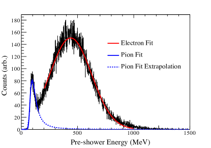
Figure 21: A signal distribution in the BigBite pre-shower, where the particle’s total deposited energy is plotted for the $<x>=0.425$ bin. Electrons (pions) are shown by the peak on the right (left). The curves fitted to the data are used in the analysis to determine the amount of pion contamination in the electron sample, see the text.

A spin asymmetry in the charged-pion production will affect the measured electron asymmetries. To study this, asymmetries in the pion sample were determined after applying corrections for the nitrogen dilution and the beam and target polarizations, yielding the $\pi^{-}$ and $\pi^{+}$ experimental asymmetries. The results are shown in Figs. 22 and 23 for $E=5.89$ GeV. After scaling these measured pion asymmetries with the $N_{\pi}/N_{e}$ ratios, it was found that the $\pi^{-}$ ($\pi^{+}$) asymmetry contribution was less than 5% (3%) of the statistical uncertainty in the asymmetries and therefore could be neglected.

Figure 22: The $\pi^{-}$ experimental asymmetry on ³He for $E=5.89$ GeV. The left (right) panel shows the data for the target polarized longitudinal (transverse) to the electron beam momentum. The error bars indicate the statistical uncertainty.

Figure 23: The $\pi^{+}$ experimental asymmetry on ³He for $E=5.89$ GeV. The left (right) panel shows the data for the target polarized longitudinal (transverse) to the electron beam momentum. The error bars indicate the statistical uncertainty.

To quantify the contamination due to pair-produced electrons, the ratio of positrons to electrons, $N_{e^{+}}/N_{e^{-}}$ needed to be determined. Due to time constraints this ratio could only be measured directly at 4.74 GeV. To determine this ratio for the 5.89 GeV run a parametrization was made of the 4.74 GeV BigBite and LHRS runs, the 5.89 GeV LHRS run together with data at 5.7 GeV and $\theta=41.1^{\circ}$ from JLab CLAS EG1b Bosted (2004). These data, multiplied by $(1/E^{2})(N_{e^{+}}/N_{e^{-}})$, were then fit to an empirical function $f(k_{T})=\exp(a+b\cdot k_{T})$ with $k_{T}=k\sin\theta$ being the transverse momentum. The data and the fit are shown in Fig. 24. The error on the fit was propagated to be 5–6% across the $x$-range of the measurements. The lowest $x$ bin, $x=0.23$, was then excluded from further analysis after the $N_{e^{+}}/N_{e^{-}}$ ratio was found to be in excess of 80%. At the first bin included in the analysis, $x=0.277$, that ratio was $\sim 50$% and fell to less than 10% by $x=0.473$. Beyond $x=0.5$ the ratio had dropped to below 3% Posik (2013).

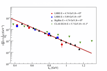
Figure 24: (Color online) The $N_{e^{+}}/N_{e^{-}}$ data from this experiment measured in the LHRS and BigBite and CLAS EG1b Bosted (2004) plotted as $(1/E^{2})(N_{e^{+}}/N_{e^{-}})$ versus the transverse momentum $k_{T}$. Our fit function is shown by the solid curve, with its error given by the band surrounding it. See text for additional details.

Just as with the pion contamination, pair-produced electrons can affect or dilute the measured electron asymmetry. Ideally, the asymmetry should be measured by reversing the polarity of BigBite so that the positrons are detected with the same acceptance as the electrons. However, due to the same time constraints as mentioned previously, this could only be completed for one target-spin orientation ($270^{\circ}$) at 4.74 GeV. Because of this, the positron asymmetries were measured bent down in BigBite. The asymmetries measured in this configuration were observed to be in good agreement with those when the positrons were deflected upwards; however, the acceptance, and hence the rate, was $\sim 60$% lower. Therefore, for each beam energy and each target-spin configuration a weighted average was computed over all measured asymmetries. The results are shown in Figs 25 and 26. The measured electron asymmetries for each beam energy and target spin-configuration were then corrected by the corresponding weighted average positron asymmetry scaled by the $N_{e^{+}}/N_{e^{-}}$ ratio.

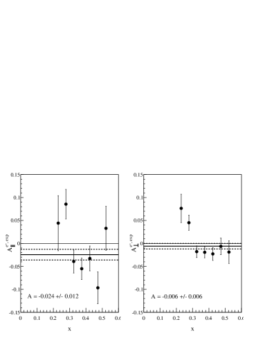
Figure 25: The positron experimental asymmetry for $E=4.74$ GeV. The left (right) panel shows the data for the target polarized longitudinal (transverse) to the electron beam momentum. The error bars indicate the statistical uncertainty. The weighted average is indicated by the solid line, and its uncertainty is indicated by the surrounding dashed lines. The numerical value of the weighted average with its uncertainty is also shown.

Figure 26: The positron experimental asymmetry for $E=5.89$ GeV. The desciption of the data and fitted line with its uncertainty is the same as Fig. 25.

The effects of the charged-pion and pair-produced electron asymmetries were corrected for through:

$$A_{e^{-}}=\frac{A^{\text{exp}}_{e^{-}}-f_{1}A^{\text{exp}}_{\pi^{-}}-f_{3}A^{\text{exp}}_{e^{+}}+f_{2}f_{3}A^{\text{exp}}_{\pi^{+}}}{1-f_{1}-f_{3}+f_{2}f_{3}},$$ (36)

where $f_{1}=N_{\pi^{-}}/N_{e^{-}}$; $f_{2}=N_{\pi^{+}}/N_{e^{+}}$; $f_{3}=N_{e^{+}}/N_{e^{-}}$; $A^{\text{exp}}_{\pi^{\pm}}$ are the $\pi^{\pm}$ experimental asymmetries, and $A^{\text{exp}}_{e^{+}}$ is the positron experimental asymmetry. Since the corrections for the pion experimental asymmetries were found to be negligible, Eq. 36 can be simplified to:

$$A_{e^{-}}\approx\frac{A^{\text{exp}}_{e^{-}}-f_{3}A^{\text{exp}}_{e^{+}}}{1-f_{1}-f_{3}+f_{2}f_{3}}\equiv A^{\text{cor}}.$$ (37)

At this point, the bins for which $x>0.90$ were removed from the analysis, so as to exclude the quasi-elastic and $\Delta$ resonance contributions.

IV.3.4 False asymmetries

When measuring a scattering asymmetry, care must be taken to ensure that the asymmetry was due to electron spin-dependent scattering and not to helicity-correlated changes in the electron beam, known as false asymmetries. One potential false asymmetry arises from a difference in the electron beam intensity between the two helicity states, resulting in an asymmetry in the deposited charge on the target. During the experiment, the beam charge asymmetry was limited to $\sim 100$ ppm through the use of a feedback loop controlled by a specialized DAQ Michaels and Moffit and was verified by measuring the charge asymmetry using the Compton polarimeter Parno (2011). Compared to the size of the electron asymmetry measurements, $A^{\text{cor}}$, the charge asymmetry was negligible.

Helicity-dependent DAQ changes can also generate false asymmetries, which can be observed through the measurement of the detector’s live-time. A helicity-dependent rate change could lead to one helicity state having a larger live-time than the other, resulting in an asymmetry. BigBite detector live-times were recorded for each helicity gate for each run of the experiment. The helicity-dependent live-time asymmetry was extracted from the data and was found to be $<100$ ppm for the entire data set, which was negligible Posik (2013).

In addition to charge- and DAQ-induced false asymmetries, the analysis could also introduce a false asymmetry. For example, if the data rates were high enough, it may be more difficult to reconstruct good tracks related to the higher-rate helicity state as compared to the lower-rate one, resulting in an asymmetry Riordan (2008). However, the E06-014 data set was dominated by single-track events ($\sim 96\%$), and thus the rates were not high enough for such an asymmetry to have a significant impact on the measured electron asymmetries.

Potential sources of false asymmetries are limited by the 30 Hz helicity flipping rate of the electron beam. Additionally, any false asymmetry that does not change sign with respect to the IHWP state (Section IV.3.1), such as those due to electronic cross-talk Miller (2001), would be canceled when combining data from the two IHWP states. In summary, no significant false asymmetries were observed.

IV.3.5 Radiative corrections

Radiative corrections on the asymmetries were applied utilizing a similar approach as on the cross sections in Section IV.2.3. We carried out the corrections on polarized cross section differences, $\Delta\sigma$, related to asymmetries by:

$$A_{\parallel,\perp}^{r}=\frac{\Delta\sigma_{\parallel,\perp}^{r}}{2\sigma_{0}^{r}},$$ (38)

where $A_{\parallel}^{r}$ ($A_{\perp}^{r}$) indicates the longitudinal (perpendicular) asymmetry which includes radiative effects. The unpolarized cross section is $\sigma_{0}^{r}$, where the $r$ indicates that radiative effects have been applied. We used the F1F209 parameterization Bosted and Mamyan (2012) for the unpolarized cross section. The input used to fill out the integration phase space fell into three different kinematic regions: the DIS region, the quasi-elastic region, and the $\Delta$ resonance region. For the DIS region the DSSV de Florian et al. (2008) PDF parametrization was used, for the quasi-elastic region Bosted’s nucleon form factors Bosted (1995), smeared by a quasi-elastic scaling function Amaro et al. (2005) was used and for the $\Delta$ region the MAID model Drechsel et al. (2007) was used. The $\Delta\sigma$ obtained after putting these models together for the three regions described the JLab E94-010 data Amarian et al. (2002); *Slifer:2008re reasonably well Flay (2014).

In the radiative correction procedure, the quasi-elastic tail was not subtracted first, but rather included in the integration. The elastic tail was found to be negligible and was not subtracted. To minimize statistical fluctuations in the radiative corrections, the corrections were performed on a model of our data set. After obtaining the final $\Delta\sigma$, the corresponding asymmetry was obtained by inverting Eq. 38 (but using the Born $\sigma_{0}$ from F1F209) to find $A$ with the size of the radiative correction given by:

$$\Delta A=A^{b}-A^{r}.$$ (39)

The quantity $A^{b}$ denotes the Born asymmetry and $A^{r}$ the radiated asymmetry. Here, $A^{r}$ is the model input to the radiative corrections program. This $\Delta A$ was applied to our extracted asymmetries, $A_{\parallel,\perp}^{\text{cor}}$ (see Eq. 37), as an additive correction. The size of the radiative correction was found to be at most of the order of 45% (10^-3 absolute) of the uncorrected asymmetry. The radiative corrections in the DIS region were checked against results obtained using the formalism of Akushevich et al. Akushevich et al. (1997). The results of both methods agreed to the $10^{-4}$ level in the asymmetry.

The asymmetries on ³He before and after radiative corrections for the 4.74 and 5.89 GeV runs are shown in Figs. 27 and 28 and tabulated in Tables 6 and 7 in Section V. The systematic uncertainties for the radiative corrected data, were obtained by varying all input to reasonable levels. The inputs varied included the electron cuts, the nitrogen dilution factor, beam and target polarizations, pion and pair-production contamination levels and the radiative corrections. The latter were observed to change less than 5% when using various input models and when the radiation thicknesses before and after scattering were varied by up to $\pm 10$%. Tables in Appendix E.2 list the various contributions to the systematic errors.

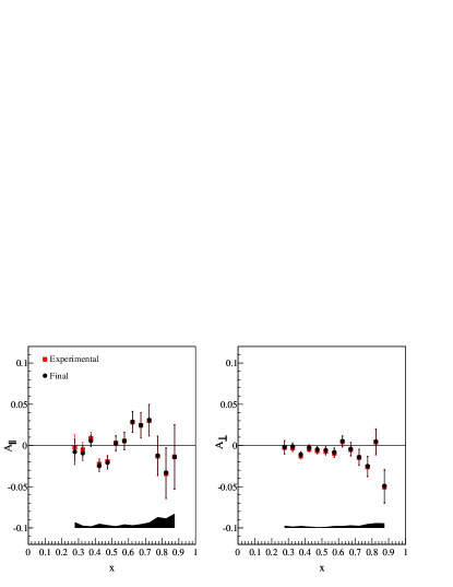
Figure 27: (Color online) The parallel and perpendicular asymmetries on ³He for $E=4.74$ GeV before (square) and after (circle) radiative corrections. The error bands indicate the systematic uncertainty for the final asymmetries.

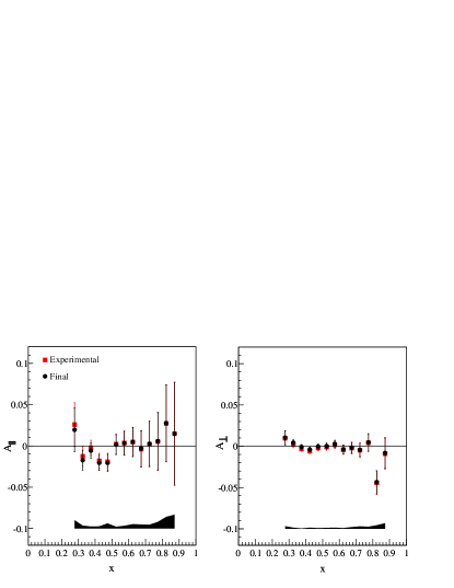
Figure 28: (Color online) The parallel and perpendicular asymmetries on ³He for $E=5.89$ GeV before (square) and after (circle) radiative corrections. The error bands indicate the systematic error for the final asymmetries.

IV.4 From ³He to the neutron

Free nucleons behave differently from those bound in nuclei, primarily due to spin depolarization, Fermi motion, nuclear binding, and nuclear shadowing and anti-shadowing effects. Additionally, the characteristics of bound nucleons can be altered by the presence of non-nucleonic degrees of freedom and how far off-shell the nucleons are.

We utilized the work of Bissey et. al. Bissey et al. (2002), which provides a description of the $g_{1}$ spin structure function on ³He over the range $10^{-4}\leq x\leq 0.8$. It models the ³He wavefunction incorporating the $S$, $S^{\prime}$ and $D$ states, and includes a pre-existing $\Delta$ (1232) component:

$$g_{1}^{{}^{3}\text{He}}(x) = P_{n}g_{1}^{n}(x)+2P_{p}g_{1}^{p}(x)-0.014\left[g_{1}^{p}(x)-4g_{1}^{n}(x)\right]$$ (40)

$$+ a(x)g_{1}^{n}(x)+b(x)g_{1}^{p}(x),$$

where $P_{p}$ and $P_{n}$ are the effective polarizations of the proton and neutron in ³He Friar et al. (1990), respectively. The third term arises from the $\Delta(1232)$ component in the ³He wave function Bissey et al. (2002). The functions $a(x)$ and $b(x)$ describe nuclear shadowing and anti-shadowing effects. In the present experiment, the $x$-coverage does not drop below $x\sim 0.2$ so that shadowing and anti-shadowing effects can be neglected. Therefore, Eq. 40 becomes:

$$g_{1}^{{}^{3}\text{He}}(x)\approx P_{n}g_{1}^{n}(x)+2P_{p}g_{1}^{p}(x)-0.014\left[g_{1}^{p}(x)-4g_{1}^{n}(x)\right].$$ (41)

The same formula applies for $g_{2}$ data, with $g_{2}$ replacing $g_{1}$ in Eq. 41.

The nuclear corrections to our data for $d_{2}^{{}^{3}\text{He}}$ were applied to the integral (not bin-by-bin to the $d_{2}$ integrand), which resulted in two average $Q^{2}$-bins for each of the beam energies 4.74 and 5.89 GeV. Thus, the correction followed the formalism defined in Eq. 41:

$$d_{2}^{n}=\frac{1}{\tilde{P}_{n}}\left(d_{2}^{{}^{3}\text{He}}-\tilde{P}_{p}d_{2}^{p}\right),$$ (42)

for a given bin in $Q^{2}$, where the quantity $\tilde{P}_{p}=2P_{p}-0.014$ and $\tilde{P}_{n}=P_{n}+0.056$. For the proton an effective polarization $P_{p}=-0.028^{+0.009}_{-0.004}$ was used, and for the neutron $P_{n}=0.86^{+0.036}_{-0.020}$ Zheng et al. (2004a). The matrix element $d_{2}^{p}$ was evaluated by considering various global analyses de Florian et al. (2008); Bourrely et al. (2002, 2007); Leader et al. (1998); de Florian et al. (2005); Gehrmann and Stirling (1996) to construct $g_{1}^{p}$. The Wandzura-Wilczek relation Wandzura and Wilczek (1977); Accardi et al. (2009a, b) was used to obtain $g_{2}^{p}$, which is valid if the higher-twist effects are assumed to be small; this is a reasonable assumption based on the results of SLAC E155 Anthony et al. (1999). Using the average of the results for $g_{1}^{p}$ and $g_{2}^{p}$, the $d_{2}^{p}$ integral was evaluated over the same $x$-range of our experiment at $\left<Q^{2}\right>=3.21$ and $4.32$ GeV², and the result was inserted into Eq. 42.

To obtain the nuclear corrections needed to extract $g_{1}^{n}/F_{1}^{n}$, we first divided Eq. 41 by $F_{1}^{{}^{3}\text{He}}$ and then rewrote $F_{1}^{{}^{3}\text{He}}$ in terms of $F_{2}^{{}^{3}\text{He}}$ following:

$$F_{1}\left(x,Q^{2}\right)=\frac{F_{2}\left(x,Q^{2}\right)\left(1+\gamma^{2}\right)}{2x\left[1+R\left(x,Q^{2}\right)\right]},$$ (43)

where $R$ is taken to be target-independent Bissey et al. (2002), which is a reasonable assumption for $Q^{2}>1.5$ GeV² and $x>0.15$ Ackerstaff et al. (2000). Solving for $g_{1}^{n}/F_{1}^{n}$ yielded:

$$\frac{g_{1}^{n}}{F_{1}^{n}}=\frac{1}{\tilde{P}_{n}}\frac{F_{2}^{{}^{3}\text{He}}}{F_{2}^{n}}\left(\frac{g_{1}^{{}^{3}\text{He}}}{F_{1}^{{}^{3}\text{He}}}-\tilde{P}_{p}\frac{F_{2}^{p}}{F_{2}^{{}^{3}\text{He}}}\frac{g_{1}^{p}}{F_{1}^{p}}\right).$$ (44)

Using Eq. 44, we extracted $g_{1}^{n}/F_{1}^{n}$ from our ³He data. For the unpolarized $F_{2}^{{}^{3}\text{He}}$ structure function, we utilized the F1F209 parameterization Bosted and Mamyan (2012), which incorporates Fermi motion and EMC effects, and for $F_{2}^{p}$ and $F_{2}^{n}$, the unpolarized PDF model CJ12 Owens et al. (2013) to world data was used. A fit to world $g_{1}^{p}/F_{1}^{p}$ data Ackerstaff et al. (1997); Abe et al. (1998); Anthony et al. (1999); Dharmawardane et al. (2006); Prok et al. (2014) was performed and used. The fit used a second-order polynomial in $x$ with three free parameters and assumed $Q^{2}$-independence. Any $Q^{2}$-dependence would cancel in the ratio of $g_{1}/F_{1}$ to leading order and next-to-leading order Anselmino et al. (1995). For more details, see Appendix C.2.

For the nuclear corrections to obtain $A_{1}^{n}$, we used the expression for $A_{1}$ in terms of the structure functions $g_{1}$, $g_{2}$ and $F_{1}$ (Appendix A.4). Solving for $A_{1}^{n}$ gave (cf. Eq. 44):

$$A_{1}^{n}=\frac{1}{\tilde{P}_{n}}\frac{F_{2}^{{}^{3}\text{He}}}{F_{2}^{n}}\left(A_{1}^{{}^{3}\text{He}}-\tilde{P}_{p}\frac{F_{2}^{p}}{F_{2}^{{}^{3}\text{He}}}A_{1}^{p}\right).$$ (45)

The same models used in the $g_{1}/F_{1}$ analysis for $F_{2}$ on ³He, the proton and the neutron were used in the $A_{1}$ analysis. Similar to the $g_{1}/F_{1}$ analysis, a $Q^{2}$-independent, second-order polynomial in $x$ was fit to world $A_{1}^{p}$ data Airapetian et al. (2007); Abe et al. (1998); Anthony et al. (1999); Ashman et al. (1988, 1989); Dharmawardane et al. (2006); Alekseev et al. (2010b); Adeva et al. (1998) and used in the analysis. For more details, see Appendix C.3.

Other neutron extraction methods have been studied in Ref. Ethier and Melnitchouk (2013), where the full convolution formalism was used at finite $Q^{2}$, including the nucleon off-shell and $\Delta$ contributions. Such calculations are consistent with our extraction of $d_{2}^{n}$ and $A_{1}^{n}$ following Eqs. 42 and 45, respectively.

V Results

V.1 ³He results

Results for the unpolarized $e$-³He scattering cross section (Section IV.2) for $E=4.74$ and $5.89$ GeV are given in Tables 4 and 5. All of the contributions to the systematic uncertainty in the cross section are given in Tables 23 and 24. The biggest contribution to the systematic uncertainty was the background subtraction, at a relative uncertainty of $\sim 9$% in the lowest bin in $x$. Our extracted cross section values are in good agreement with the F1F209 parameterization Bosted and Mamyan (2012).

Table 4: The final ³He unpolarized cross sections for 4.74 GeV data. The uncertainties listed are statistical and systematic, respectively.

$\left<x\right>$	$\left<Q^{2}\right>$ (GeV2)	$\frac{d^{3}\sigma}{d\Omega dE^{\prime}}$ (nb/GeV/sr)
0.214	1.659	6.191 $\pm$ 0.365 $\pm$ 0.561
0.299	2.209	5.374 $\pm$ 0.178 $\pm$ 0.281
0.456	3.094	2.544 $\pm$ 0.048 $\pm$ 0.121
0.494	3.285	2.223 $\pm$ 0.034 $\pm$ 0.103
0.533	3.472	1.762 $\pm$ 0.026 $\pm$ 0.084
0.579	3.694	1.353 $\pm$ 0.027 $\pm$ 0.065
0.629	3.909	1.021 $\pm$ 0.018 $\pm$ 0.050
0.686	4.149	0.718 $\pm$ 0.012 $\pm$ 0.035
0.745	4.387	0.536 $\pm$ 0.012 $\pm$ 0.028

Table 5: The final ³He unpolarized cross sections for 5.89 GeV data. The uncertainties listed are statistical and systematic, respectively.

$\left<x\right>$	$\left<Q^{2}\right>$ (GeV2)	$\frac{d^{3}\sigma}{d\Omega dE^{\prime}}$ (nb/GeV/sr)
0.208	2.064	4.069 $\pm$ 0.440 $\pm$ 0.492
0.247	2.409	4.322 $\pm$ 0.116 $\pm$ 0.310
0.330	3.095	2.488 $\pm$ 0.099 $\pm$ 0.130
0.434	3.882	1.596 $\pm$ 0.038 $\pm$ 0.079
0.468	4.124	1.234 $\pm$ 0.030 $\pm$ 0.063
0.503	4.360	1.067 $\pm$ 0.020 $\pm$ 0.052
0.539	4.603	0.846 $\pm$ 0.016 $\pm$ 0.042
0.580	4.873	0.679 $\pm$ 0.012 $\pm$ 0.033
0.629	5.173	0.472 $\pm$ 0.010 $\pm$ 0.022
0.679	5.478	0.331 $\pm$ 0.007 $\pm$ 0.016
0.738	5.811	0.250 $\pm$ 0.006 $\pm$ 0.013

The $\vec{e}$-${}^{3}\vec{\text{He}}$ electron asymmetries $A_{\parallel}^{{}^{3}\text{He}}$ and $A_{\perp}^{{}^{3}\text{He}}$ (Section IV.3), the virtual photon asymmetry $A_{1}^{{}^{3}\text{He}}$, and the structure function ratio $g_{1}^{{}^{3}\text{He}}/F_{1}^{{}^{3}\text{He}}$ (Eqs. 18 and 19) for the 4.74 GeV and 5.89 GeV data are given in Tables 6 and 7. The polarized structure functions $g_{1}^{{}^{3}\text{He}}$ and $g_{2}^{{}^{3}\text{He}}$ (Eqs. 74 and B.2) are given in Tables 8 and 9. All of the contributions to the systematic uncertainties are given in Appendix E, with the dominant one being the selection of the electron sample.

The asymmetry $A_{1}^{{}^{3}\text{He}}$ is plotted in Fig. 29, compared to the world DIS data from SLAC E142 Anthony et al. (1996), HERMES Ackerstaff et al. (1999) and JLab E99-117 Zheng et al. (2004b, a). Also plotted are resonance data from JLab E01-012 Solvignon et al. (2008). We find that our results reproduce the trend of existing data.

The spin-structure functions $g_{1}^{{}^{3}\text{He}}$ and $g_{2}^{{}^{3}\text{He}}$ are presented in Figs. 30 and 31, in which the world DIS data from JLab E99-117 Zheng et al. (2004b, a) and SLAC E142 Anthony et al. (1996) are also shown. Resonance data from JLab E01-012 Solvignon et al. (2008) are also presented. The gray band represents an envelope encompassing a number of global analyses de Florian et al. (2008); Gehrmann and Stirling (1996); Leader et al. (2007); de Florian et al. (2005); Bourrely et al. (2002); *Bourrely:2007if. Our data reproduce the trend seen in existing $g_{1}^{{}^{3}\text{He}}$ data. For $g_{2}^{{}^{3}\text{He}}$, our data have improved on the uncertainty by about a factor of 2 relative to the JLab E99-117 data set.

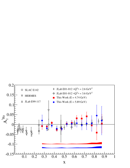
Figure 29: (Color online) Our measured result for $A_{1}^{{}^{3}\text{He}}$ for 4.74 GeV (filled squares) and 5.89 GeV (filled circles) data. The error bars on our data points represent the statistical uncertainty. The bands at the bottom of the plot indicate the systematic uncertainty for each data set, where the upper (lower) band corresponds to the 4.74 GeV (5.89 GeV) data set. The DIS data set corresponds to data for which $x<0.519$ ($x<0.623$) for $E=4.74$ GeV (5.89 GeV); the data at larger $x$ values correspond to the resonance region. Also plotted are world DIS data from SLAC E142 Anthony et al. (1996), HERMES Ackerstaff et al. (1999) and JLab E99-117 Zheng et al. (2004b, a), and resonance data from JLab E01-012 Solvignon et al. (2008).

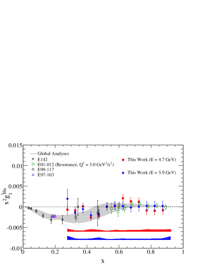
Figure 30: (Color online) Our results for $g_{1}$ on ³He for 4.74 GeV (filled squares) and 5.89 GeV (filled circles) data. The error bars on our data points represent the statistical uncertainty. The bands at the bottom of the plot indicate the systematic uncertainty for each data set, where the upper (lower) band corresponds to the 4.74 GeV (5.89 GeV) data set. The DIS data set corresponds to data for which $x<0.519$ ($x<0.623$) for $E=4.74$ GeV (5.89 GeV); the data at larger $x$ values correspond to the resonance data. Our data are compared to world DIS data from JLab E99-117 Zheng et al. (2004b, a), SLAC E142 Anthony et al. (1996), and resonance data from JLab E01-012 Solvignon et al. (2008) and JLab E97-103 Kramer (2003); Kramer et al. (2005). The gray band represents an envelope of various global analyses de Florian et al. (2008); Gehrmann and Stirling (1996); Leader et al. (2007); de Florian et al. (2005); Bourrely et al. (2002); *Bourrely:2007if for $g_{1}$ at $Q^{2}=4.43$ GeV${}^{\text{2}}$, which was the average $Q^{2}$ of our data set.

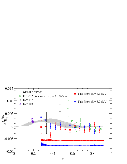
Figure 31: (Color online) Our results for $g_{2}$ on ³He for the 4.74 GeV (filled squares) and 5.89 GeV (filled circles) data. The error bars on our data points represent the statistical uncertainty. The bands at the bottom of the plot indicate the systematic uncertainty for each data set, where the upper (lower) band corresponds to the 4.74 GeV (5.89 GeV) data set. The DIS data set corresponds to data for which $x<0.519$ ($x<0.623$) for $E=4.74$ GeV (5.89 GeV); the data at larger $x$ values correspond to the resonance data. Our data are compared to world data from JLab E99-117 Zheng et al. (2004b, a), JLab E01-012 Solvignon et al. (2008) (resonance data) and JLab E97-103 Kramer (2003); Kramer et al. (2005) (resonance data). The gray band represents an envelope of various global analyses de Florian et al. (2008); Gehrmann and Stirling (1996); Leader et al. (2007); de Florian et al. (2005); Bourrely et al. (2002); *Bourrely:2007if used to construct $g_{2}^{\text{WW}}$.

Table 6: Asymmetry results for $A_{\parallel}^{{}^{3}\text{He}}$, $A_{\perp}^{{}^{3}\text{He}}$, $A_{1}^{{}^{3}\text{He}}$ and $g_{1}^{{}^{3}\text{He}}/F_{1}^{{}^{3}\text{He}}$ for the 4.74 GeV data. The first uncertainty is statistical, while the second is systematic.

$\left<x\right>$	$\left<Q^{2}\right>$ (GeV2)	$A_{\parallel}^{{}^{3}\text{He}}$	$A_{\perp}^{{}^{3}\text{He}}$	$A_{1}^{{}^{3}\text{He}}$	$g_{1}^{{}^{3}\text{He}}/F_{1}^{{}^{3}\text{He}}$
0.277	2.038	$-0.008\pm 0.015\pm 0.007$	$-0.002\pm 0.008\pm 0.003$	$-0.008\pm 0.017\pm 0.004$	$-0.009\pm 0.016\pm 0.004$
0.325	2.347	$-0.009\pm 0.009\pm 0.003$	$-0.001\pm 0.005\pm 0.002$	$-0.010\pm 0.010\pm 0.001$	$-0.010\pm 0.009\pm 0.001$
0.374	2.639	$0.005\pm 0.007\pm 0.002$	$-0.011\pm 0.004\pm 0.002$	$0.008\pm 0.008\pm 0.001$	$0.001\pm 0.007\pm 0.001$
0.424	2.915	$-0.025\pm 0.007\pm 0.005$	$-0.003\pm 0.004\pm 0.002$	$-0.027\pm 0.008\pm 0.003$	$-0.026\pm 0.007\pm 0.002$
0.473	3.176	$-0.021\pm 0.008\pm 0.003$	$-0.005\pm 0.004\pm 0.001$	$-0.022\pm 0.009\pm 0.002$	$-0.023\pm 0.008\pm 0.002$
0.523	3.425	$0.002\pm 0.009\pm 0.002$	$-0.006\pm 0.005\pm 0.001$	$0.004\pm 0.010\pm 0.001$	$0.000\pm 0.009\pm 0.001$
0.574	3.662	$0.005\pm 0.010\pm 0.004$	$-0.008\pm 0.005\pm 0.002$	$0.008\pm 0.012\pm 0.002$	$0.002\pm 0.011\pm 0.002$
0.623	3.886	$0.029\pm 0.013\pm 0.003$	$0.005\pm 0.007\pm 0.002$	$0.031\pm 0.015\pm 0.002$	$0.031\pm 0.013\pm 0.002$
0.673	4.099	$0.025\pm 0.015\pm 0.005$	$-0.004\pm 0.009\pm 0.003$	$0.030\pm 0.018\pm 0.003$	$0.023\pm 0.016\pm 0.002$
0.723	4.307	$0.031\pm 0.019\pm 0.007$	$-0.014\pm 0.009\pm 0.002$	$0.041\pm 0.022\pm 0.004$	$0.026\pm 0.020\pm 0.003$
0.773	4.504	$-0.012\pm 0.024\pm 0.013$	$-0.025\pm 0.012\pm 0.005$	$-0.005\pm 0.028\pm 0.008$	$-0.023\pm 0.025\pm 0.007$
0.823	4.694	$-0.033\pm 0.030\pm 0.012$	$0.005\pm 0.016\pm 0.006$	$-0.041\pm 0.037\pm 0.007$	$-0.032\pm 0.032\pm 0.006$
0.874	4.876	$-0.014\pm 0.039\pm 0.017$	$-0.049\pm 0.020\pm 0.006$	$0.004\pm 0.048\pm 0.010$	$-0.035\pm 0.041\pm 0.009$

Table 7: Asymmetry results for $A_{\parallel}^{{}^{3}\text{He}}$, $A_{\perp}^{{}^{3}\text{He}}$, $A_{1}^{{}^{3}\text{He}}$ and $g_{1}^{{}^{3}\text{He}}/F_{1}^{{}^{3}\text{He}}$ for the 5.89 GeV data. The first uncertainty is statistical, while the second is systematic.

$\left<x\right>$	$\left<Q^{2}\right>$ (GeV2)	$A_{\parallel}^{{}^{3}\text{He}}$	$A_{\perp}^{{}^{3}\text{He}}$	$A_{1}^{{}^{3}\text{He}}$	$g_{1}^{{}^{3}\text{He}}/F_{1}^{{}^{3}\text{He}}$
0.277	2.626	$0.019\pm 0.027\pm 0.010$	$0.010\pm 0.008\pm 0.003$	$0.020\pm 0.029\pm 0.006$	$0.024\pm 0.028\pm 0.006$
0.325	3.032	$-0.017\pm 0.012\pm 0.003$	$0.004\pm 0.004\pm 0.001$	$-0.019\pm 0.013\pm 0.002$	$-0.016\pm 0.012\pm 0.002$
0.374	3.421	$-0.006\pm 0.009\pm 0.002$	$-0.001\pm 0.003\pm 0.001$	$-0.006\pm 0.010\pm 0.001$	$-0.006\pm 0.009\pm 0.001$
0.424	3.802	$-0.020\pm 0.009\pm 0.003$	$-0.004\pm 0.003\pm 0.001$	$-0.021\pm 0.010\pm 0.002$	$-0.022\pm 0.009\pm 0.002$
0.474	4.169	$-0.021\pm 0.010\pm 0.006$	$0.000\pm 0.003\pm 0.001$	$-0.022\pm 0.011\pm 0.003$	$-0.021\pm 0.010\pm 0.003$
0.524	4.514	$0.002\pm 0.012\pm 0.002$	$0.000\pm 0.004\pm 0.001$	$0.002\pm 0.013\pm 0.001$	$0.002\pm 0.012\pm 0.001$
0.573	4.848	$0.003\pm 0.015\pm 0.003$	$0.003\pm 0.004\pm 0.001$	$0.003\pm 0.016\pm 0.002$	$0.004\pm 0.015\pm 0.002$
0.624	5.176	$0.005\pm 0.018\pm 0.005$	$-0.004\pm 0.005\pm 0.001$	$0.006\pm 0.020\pm 0.003$	$0.003\pm 0.018\pm 0.003$
0.674	5.486	$-0.003\pm 0.022\pm 0.005$	$-0.002\pm 0.007\pm 0.002$	$-0.003\pm 0.024\pm 0.003$	$-0.004\pm 0.022\pm 0.002$
0.723	5.777	$0.003\pm 0.027\pm 0.005$	$-0.004\pm 0.008\pm 0.003$	$0.004\pm 0.031\pm 0.003$	$0.001\pm 0.028\pm 0.003$
0.773	6.059	$0.006\pm 0.035\pm 0.008$	$0.005\pm 0.010\pm 0.002$	$0.005\pm 0.039\pm 0.004$	$0.008\pm 0.035\pm 0.004$
0.823	6.325	$0.028\pm 0.047\pm 0.014$	$-0.044\pm 0.014\pm 0.004$	$0.045\pm 0.053\pm 0.008$	$0.009\pm 0.047\pm 0.013$
0.873	6.585	$0.015\pm 0.062\pm 0.017$	$-0.008\pm 0.019\pm 0.007$	$0.020\pm 0.072\pm 0.009$	$0.011\pm 0.064\pm 0.009$

Table 8: The $g_{1}$ and $g_{2}$ spin-structure functions measured on ³He at an incident electron energy of 4.74 GeV. The first uncertainty is statistical, while the second is systematic.

$\left<x\right>$	$g_{1}^{{}^{3}\text{He}}$	$g_{2}^{{}^{3}\text{He}}$
0.277	$-0.009\pm 0.016\pm 0.009$	$-0.006\pm 0.034\pm 0.009$
0.325	$-0.009\pm 0.008\pm 0.002$	$-0.001\pm 0.014\pm 0.006$
0.374	$0.001\pm 0.005\pm 0.002$	$-0.026\pm 0.009\pm 0.005$
0.424	$-0.014\pm 0.004\pm 0.003$	$0.001\pm 0.006\pm 0.002$
0.473	$-0.010\pm 0.003\pm 0.002$	$-0.002\pm 0.004\pm 0.001$
0.523	$0.000\pm 0.003\pm 0.000$	$-0.005\pm 0.004\pm 0.001$
0.574	$0.000\pm 0.003\pm 0.001$	$-0.005\pm 0.003\pm 0.001$
0.623	$0.005\pm 0.002\pm 0.001$	$0.000\pm 0.002\pm 0.001$
0.673	$0.003\pm 0.002\pm 0.001$	$-0.002\pm 0.002\pm 0.001$
0.723	$0.002\pm 0.002\pm 0.001$	$-0.003\pm 0.002\pm 0.001$
0.773	$-0.001\pm 0.002\pm 0.001$	$-0.002\pm 0.001\pm 0.001$
0.823	$-0.001\pm 0.001\pm 0.001$	$0.001\pm 0.001\pm 0.000$
0.874	$-0.001\pm 0.001\pm 0.001$	$-0.002\pm 0.001\pm 0.001$

Table 9: The $g_{1}$ and $g_{2}$ spin-structure functions measured on ³He at an incident electron energy of 5.89 GeV. The first uncertainty is statistical, while the second is systematic.

$\left<x\right>$	$g_{1}^{{}^{3}\text{He}}$	$g_{2}^{{}^{3}\text{He}}$
0.277	$0.026\pm 0.029\pm 0.012$	$0.046\pm 0.047\pm 0.019$
0.325	$-0.013\pm 0.010\pm 0.003$	$0.022\pm 0.015\pm 0.006$
0.374	$-0.004\pm 0.006\pm 0.002$	$0.000\pm 0.008\pm 0.002$
0.424	$-0.011\pm 0.005\pm 0.002$	$-0.002\pm 0.006\pm 0.002$
0.474	$-0.008\pm 0.004\pm 0.002$	$0.003\pm 0.004\pm 0.002$
0.524	$0.000\pm 0.003\pm 0.001$	$0.000\pm 0.003\pm 0.001$
0.573	$0.001\pm 0.003\pm 0.001$	$0.001\pm 0.003\pm 0.001$
0.624	$0.000\pm 0.002\pm 0.001$	$-0.002\pm 0.002\pm 0.000$
0.674	$0.000\pm 0.002\pm 0.000$	$0.000\pm 0.002\pm 0.000$
0.723	$0.000\pm 0.002\pm 0.000$	$-0.001\pm 0.002\pm 0.000$
0.773	$0.000\pm 0.002\pm 0.000$	$0.000\pm 0.001\pm 0.000$
0.823	$0.000\pm 0.002\pm 0.000$	$-0.003\pm 0.001\pm 0.001$
0.873	$0.000\pm 0.002\pm 0.000$	$0.000\pm 0.001\pm 0.000$

V.2 Neutron results

V.2.1 The matrix element $d_{2}^{n}$

Results for the $d_{2}^{n}$ matrix element (Eq. I.2 and Section IV.4), first published in Ref. Posik et al. (2014), are shown in Fig. 34 and tabulated in Table 10. The matrix element was extracted using the Cornwall-Norton (CN) moments Melnitchouk et al. (2005). Since our measurement did not cover the full $x$ range, a low-$x$ ($x<0.25$) and a high-$x$ ($x>0.90$) contribution needed to be evaluated from other sources. For the low-$x$ region, a third-order polynomial fit to the world data on $x^{2}g_{1}^{n}$ Anthony et al. (1996); Abe et al. (1998, 1997a); Kramer et al. (2005) and $x^{2}g_{2}^{n}$ Kramer et al. (2005); Anthony et al. (1999, 2003) was used to evaluate $d_{2}^{n}$. This contribution is relatively small, considering the $x^{2}$-weighting. The large-$x$ contribution comes from the elastic peak, which was modeled using the Riordan Riordan et al. (2010) and Kelly Kelly (2004) parameterizations. The contribution from the range $0.90<x<0.99$ was considered to be negligible when taking into account the size of our $g_{1}$ and $g_{2}$ data at $x\sim 0.90$. Nuclear corrections were applied to our ³He data as described in Section IV.4. Adding the low-$x$ and high-$x$ (elastic) contributions to our measured result gave the full $d_{2}^{n}$ integral. Target mass corrections (TMCs) were checked by extracting $d_{2}^{n}$ using the Nachtmann moments Nachtmann (1973); *Accardi:2008pc; *Sidorov:2006fi; *Matsuda:1979ad; *Wandzura:1977ce; the difference between the CN and Nachtmann approaches was found to be small relative to the statistical uncertainties. An overview of the systematic uncertainties is given in Table 33. The largest contribution to the systematic uncertainty comes from the unmeasured low-$x$ region.

Our unpolarized cross section and double-spin asymmetry data were obtained at various $Q^{2}$ values; since the $d_{2}^{n}$ integral is typically carried out at constant $Q^{2}$, we considered what the effect of evolving $\bar{g}_{2}^{n}$ (the twist-3 part of $g_{2}^{n}$) would have on the $d_{2}^{n}$ value. To do this, we utilized the $\bar{g}_{2}^{n}$ model from Ref. Braun et al. (2011) along with the $Q^{2}$ evolution description for $g_{2}^{n}$ from Ref. Braun et al. (2001), which uses flavor-nonsinglet evolution equations and utilizes large-$N_{c}$ and large-$x$ ($x\gtrsim 0.1$) approximations. The $Q^{2}$-evolution calculations were performed using QCDNum Botje (2011) in the variable-flavor number scheme (VFNS) and with $\alpha_{s}\left(Q^{2}=M_{Z}^{2}\right)=0.1185$ Olive et al. (2014). For each of our measured $x$ bins at a given beam energy, the model was evolved from its initial value at $Q^{2}=1$ GeV² to the measured $Q^{2}$-value $\left(Q_{m}^{2}\right)$ for that particular $x$-bin and also to the $\left<Q^{2}\right>$ value for the given beam energy, see Figs. 32 and 33. We then evaluated:

$$\Delta d_{2}^{n}=|d_{2}^{n}\left(\left<Q^{2}\right>\right)-d_{2}^{n}\left(Q_{m}^{2}\right)|$$ (46)

where $\left<Q^{2}\right>=3.21$ GeV² (4.32 GeV²) for $E=4.74$ GeV (5.89 GeV). The $d_{2}^{n}$ integral was evaluated according to Eq. 4 for our measured $\left<x\right>$ bins corresponding to $0.277\leq x\leq 0.874$ ($0.277\leq x\leq 0.873$) for $E=4.74$ GeV (5.89 GeV). We found $\Delta d_{2}^{n}=0.00008$ (0.00007) for the $E=4.74$ GeV (5.89 GeV), which is a factor of 6 (5) smaller than the systematic uncertainty on our measured $d_{2}^{n}$ for $E=4.74$ GeV (5.89 GeV). The difference between the constant $Q^{2}$ evaluation of $d_{2}^{n}$ compared to the varying $Q^{2}$ approach was taken as an estimate of the systematic uncertainty due to not performing the $Q^{2}$ evolution on our data.

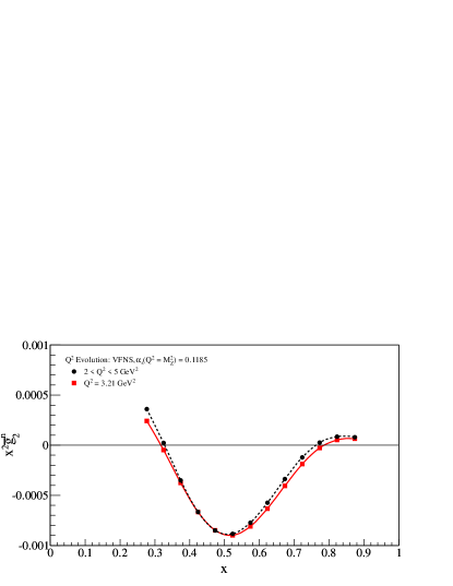
Figure 32: (Color online) The $d_{2}^{n}$ integrand for 4.74 GeV kinematics. For each measured $\left<x\right>$ bin, the model Braun et al. (2011) was evolved Braun et al. (2001); Botje (2011) to the measured (average) $Q^{2}$ value indicated by the circles (squares). For more details, see the text.

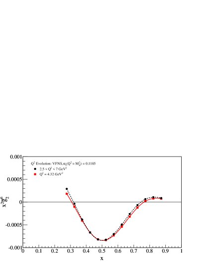
Figure 33: (Color online) The $d_{2}^{n}$ integrand for 5.89 GeV kinematics. For each measured $\left<x\right>$ bin, the model Braun et al. (2011) was evolved Braun et al. (2001); Botje (2011) to the measured (average) $Q^{2}$ value indicated by the circles (squares). For more details, see the text.

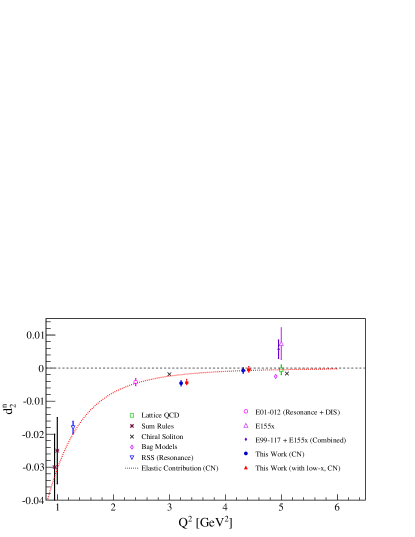
Figure 34: (Color online) Our measured $d_{2}^{n}$ data as a function of $Q^{2}$ compared to the world data from SLAC E155x Anthony et al. (2003), JLab E99-117 and SLAC E155x Zheng et al. (2004a), JLab RSS Slifer et al. (2010) and JLab E01-012 Solvignon et al. (2015). Also shown are various theoretical calculations, including a QCD sum rule approach Stein et al. (1995a); Balitsky et al. (1990), a chiral soliton model Weigel et al. (1997); *Weigel:2000gx and a bag model Song (1996). Additionally, a lattice QCD Göckeler et al. (2005) calculation is shown. The elastic contribution to $d_{2}^{n}$ is given by the dashed curve, evaluated using the CN moments. Figure reproduced from Ref. Posik et al. (2014).

Table 10: The $d_{2}^{n}$ results with statistical and systematic uncertainties. The last uncertainty represents that due to neglecting the $Q^{2}$-evolution of the $d_{2}^{n}$ integrand.

$\left<Q^{2}\right>$ $\left(\text{GeV}^{2}\right)$	$d_{2}^{n}$ $\left(\times 10^{-5}\right)$
3.21	$-421.0\pm 79.0\pm 82.0\pm 8.0$
4.32	$-35.0\pm 83.0\pm 69.0\pm 7.0$

Our result at $\left<Q^{2}\right>=3.21$ GeV² is small and negative, while the result at $\left<Q^{2}\right>=4.32$ GeV² is consistent with zero (Table 10). The trend of our measurements appears to be in agreement with the lattice QCD calculation Göckeler et al. (2005) at $Q^{2}=5$ GeV². Our $d_{2}^{n}$ extraction is also consistent with bag Song (1996); Stratmann (1993); Ji and Unrau (1994) and chiral soliton Weigel et al. (1997); *Weigel:2000gx models, as shown in Fig. 34.

The Jefferson Lab Angular Momentum (JAM) collaboration has published new results from their global QCD analysis Sato et al. (2016). Their work utilizes an iterative Monte Carlo technique that aims to reduce the influence of unphysical fitting parameters and lower the impact of parameter initial values on the results. JAM has included our data in their global analysis by fitting directly our DIS data for $A_{\parallel}^{{}^{3}\text{He}}$ and $A_{\perp}^{{}^{3}\text{He}}$. Extracting a pure twist-3 $d_{2}^{n}$ without higher-twist contributions from resonances at the same $Q^{2}$ values as our results, they find a sizable effect on their (extrapolated) prediction at $Q^{2}=1$ GeV², reducing it from $0.005\pm 0.005$ to $-0.001\pm 0.001$. They also found their $d_{2}^{n}$ value to be consistent with lattice calculations Göckeler et al. (2005) when extrapolating to $Q^{2}=5$ GeV².

V.2.2 The matrix element $a_{2}^{n}$

Following a similar procedure to that discussed for $d_{2}$, we can extract the $a_{2}$ matrix element from our $g_{1}$ data according to the third CN moment of $g_{1}$:

$$a_{2}\left(Q^{2}\right)=\int_{0}^{1}x^{2}g_{1}\left(x,Q^{2}\right)dx.$$ (47)

The low-$x$, high-$x$ and measured regions were treated in the same way as was done for the $d_{2}$ analysis, using the same model inputs. Our $g_{1}$ data were not evolved to a constant $Q^{2}$, as our investigation into the $Q^{2}$ evolution of our $g_{1}$ data revealed that the $Q^{2}$ dependence was negligible Posik (2013). Our results for $a_{2}^{n}$ are shown in Fig. 35, where the inner error bars are the statistical uncertainties and the outer error bars represent the in-quadrature sum of statistical and systematic uncertainties. The circle (square) data points exclude (include) the unmeasured low-$x$ region. Both data points extracted are positive, and the elastic contribution is sizable. The SLAC E143 Abe et al. (1998) data are also plotted, where their uncertainty is the in-quadrature sum of the statistical and systematic contributions. The up-triangles represent the average over global analyses de Florian et al. (2008); Bourrely et al. (2002, 2007); Gehrmann and Stirling (1996); de Florian et al. (2005); Leader et al. (2007). The lattice calculation shown is from Göckeler et al. Göckeler et al. (2005), where the error bar is statistical with a 15% systematic uncertainty added in quadrature. The systematic uncertainty arises from their extrapolation of their result to the chiral limit Göckeler et al. (2005). Our results are tabulated in Table 11, broken down into the low-$x$, measured and high-$x$ regions. The last column shows the full extraction. The systematic uncertainties on $a_{2}^{n}$ are dominated by that in $a_{2}^{{}^{3}\text{He}}$ and that due to the parameterization of $a_{2}^{p}$. The uncertainties for $a_{2}^{n}$ are summarized in Appendix E.5.

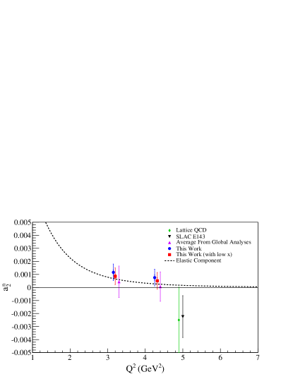
Figure 35: (Color online) Our extracted $a_{2}^{n}$ measurement compared to SLAC E143 Abe et al. (1998) and a lattice QCD calculation Göckeler et al. (2005), both of which are at $Q^{2}=5$ GeV². The lattice calculation is offset in $Q^{2}$ for clarity. The up-triangles represent the average over global analyses de Florian et al. (2008); Bourrely et al. (2002, 2007); Gehrmann and Stirling (1996); de Florian et al. (2005); Leader et al. (2007), which are offset in $Q^{2}$ for clarity. Our measurements shown as the circles (squares) exclude (include) the unmeasured low-$x$ region. The inner error bar on our data is the statistical error and the outer error bar is the in-quadrature sum of the statistical and systematic uncertainties. The results excluding the low-$x$ contribution are offset in $Q^{2}$ for clarity. The elastic contribution is computed by using the Riordan Riordan et al. (2010) and Kelly Kelly (2004) parameterizations for $G_{E}^{n}$ and $G_{M}^{n}$, respectively.

Table 11: The extracted $a_{2}^{n}$ over the full $x$-range, decomposed into the low-$x$, measured and high-$x$ components. The column labeled “full” is the sum of all three regions. The uncertainties are only listed for the full extraction, where the first quantity is the statistical uncertainty and the second is the systematic uncertainty. All uncertainties are absolute.

$\left<Q^{2}\right>$ $\left(\text{GeV}^{\text{2}}\right)$	Low-$x$ $\left(\times 10^{-4}\right)$	Measured $\left(\times 10^{-4}\right)$	High-$x$ $\left(\times 10^{-4}\right)$	Full $\left(\times 10^{-4}\right)$
3.21	$-3.056$	5.078	6.530	8.552 $\pm$ 1.761 $\pm$ 6.125
4.32	$-3.056$	5.499	2.601	5.044 $\pm$ 2.270 $\pm$ 6.042

V.2.3 Color force extraction

In order to decompose the Lorentz color force into its electric and magnetic components, one needs to first extract the twist-4 matrix element, $f_{2}^{n}$. This is accomplished by considering our measured $d_{2}^{n}$ value along with the $a_{2}^{n}$ matrix element.

The $a_{2}^{n}$ matrix element was evaluated for various global analyses de Florian et al. (2008); Bourrely et al. (2002, 2007); Gehrmann and Stirling (1996); de Florian et al. (2005); Leader et al. (2007) over the range $0.02<x<0.90$, and the average of the results at each $\left<Q^{2}\right>$-bin is taken as the value of $a_{2}^{n}$. These results are consistent with our extracted values (Fig. 35). The elastic contribution was added to the integral in a similar fashion as was done for $d_{2}^{n}$.

With $d_{2}^{n}$ and $a_{2}^{n}$ in hand, the twist-4 matrix element $f_{2}^{n}$ was evaluated following the analysis presented in Meziani et al. (2005); Ji and Melnitchouk (1997). Results for $\Gamma_{1}^{n}$ (Eq. 13) from HERMES Airapetian et al. (2003), SMC Adeva et al. (1998), JLab RSS Slifer et al. (2010) and E94-010 Slifer et al. (2008), and the SLAC experiments E142 Anthony et al. (1996), E143 Abe et al. (1998) and E154 Abe et al. (1997b) were used in the updated extraction analysis. The data sets chosen for this analysis were from those experiments that published $g_{1}^{n}$ data at constant $Q^{2}$. Since $\Gamma_{1}^{n}$ is an integral over all $x$ ($0\leq x\leq 1$), the unmeasured low-$x$ and high-$x$ regions need to be accounted for in a consistent fashion. The method we implemented for all data sets is that shown in Ref. Meziani et al. (2005), with the exception of the HERMES and JLab data, which had already used such an extrapolation. The extrapolation calls for fitting the $g_{1}^{n}$ data to an appropriate function over the appropriate $x$-range. For the low-$x$ region, the fit function was a constant $f(x)=A$, with $A$ being a free parameter. The fit was performed over the range $x_{\text{min}}<x<x^{\prime}$, where $x^{\prime}$ is the lowest measured $x$ bin for a given experiment. The lower bound $x_{\text{min}}$ is defined by $W=\sqrt{1000}$ GeV. The uncertainty in this low-$x$ extrapolation was estimated by taking the difference between our fit of $f(x)=A$ with that of a simple Regge parameterization where $f(x)=Ax^{-1/2}$ Heimann (1973); Ellis and Karliner (1988). For the high-$x$ region, the fit function was $f(x)=A(1-x)^{3}$, with $A$ being a free parameter, over the range $x^{\prime}<x<x_{\text{max}}$. The quantity $x^{\prime}$ is the highest $x$ bin for which there were data available and $x_{\text{max}}$ is defined by the pion production threshold, $W=1.12$ GeV. The fit functions for the low- and high-$x$ regions were chosen based on the trend of the data in the last three or two bins in each case, respectively.

The elastic contribution to $\Gamma_{1}^{n}$ was evaluated using the Riordan Riordan et al. (2010) and Kelly Kelly (2004) parameterizations, and was added to all of the world data. The uncertainty on the elastic contribution was estimated as the difference between using the Riordan (Kelly) parameterization for $G_{E}^{n}$ ($G_{M}^{n}$) compared to using Galster Galster et al. (1971) (dipole) for $G_{E}^{n}$ ($G_{M}^{n}$). The resulting $\Gamma_{1}^{n}$ data from this analysis are presented in Appendix D.

In order to extract the higher-twist contribution, the twist-2 contribution must first be removed. Using the OPE Wilson (1969), $\Gamma_{1}^{n}$ was expanded as an inverse power series in $Q^{2}$, revealing the higher-twist components, that was accessed by subtracting the leading twist (twist-2) contribution. The twist-2 contribution $\mu_{2}^{n}$ was calculated using Eq. 14, where $\alpha_{s}$ was parameterized according to Bethke (2009) and normalized to $\alpha_{s}\left(1\text{ GeV}^{2}\right)=0.45\pm 0.05$ for $\Lambda_{\text{QCD}}=315$ MeV. We used $N_{f}=3$ and $N_{\text{loop}}=3$ Ji and Melnitchouk (1997), $g_{A}=1.2723\pm 0.0023$ Olive et al. (2014), and $a_{8}=0.587\pm 0.016$ Olive et al. (2014). Note that the values for $g_{A}$ and $a_{8}$ have been updated relative to those used in Ref. Posik et al. (2014). At large $Q^{2}$, the higher-twist contributions should be small due to the $Q^{-2}$ suppression; therefore, $\Gamma_{1}^{n}\left(Q^{2}\right)=\mu_{2}\left(Q^{2}\right)$. Because of this, the axial charge $\Delta\Sigma$ was extracted (Eq. 14) using the highest $Q^{2}$-measurements from SLAC E154 Abe et al. (1997b) $(Q^{2}=5\text{ GeV}^{2})$, SMC Adeva et al. (1998) $(Q^{2}=10\text{ GeV}^{2})$, and HERMES Airapetian et al. (2003) $(Q^{2}=6.5\text{ GeV}^{2})$. Statistically averaging the results of these experiments yielded $Q^{2}=5.77$ GeV² and $\Gamma_{1}^{n}=-0.03851\pm 0.00535$, resulting in $\Delta\Sigma=0.375\pm 0.052$. This calculation is in excellent agreement with Accardi et al. (2012) and is consistent with Ref. de Florian et al. (2008), but at odds with Ref. Nocera et al. (2014). In the latter case, we suspect this disagreement may be due in part to differing approaches in the low-$x$ extrapolation of the world data in the various global analyses; additionally, Ref. Nocera et al. (2014) is dominated by proton data (and does not include JLab neutron data Zheng et al. (2004b, a); Solvignon et al. (2015); Slifer et al. (2008)), which may be biasing the extraction of $\Delta\Sigma$, though it is clear that there is a need for more neutron data in general.

As described in Appendix D, a fit to $\Gamma_{1}^{n}-\mu_{2}$ as a function of $Q^{2}$ allows the extraction of $f_{2}^{n}$ after inserting the average $a_{2}^{n}$ (see beginning of Section V.2.3) and $d_{2}^{n}$ from the present experiment. The extracted $f_{2}^{n}$ values are given in Table 12. This result differs from that in Ref. Posik et al. (2014) because we have improved our analysis, where we have updated the values for $g_{A}$ and $a_{8}$ used in the evaluation of the twist-2 term $\mu_{2}$. We also now include uncertainties on the low-$x$ and elastic terms in the $\Gamma_{1}^{n}$ analysis mentioned above; additionally, our uncertainty on $f_{2}^{n}$ has changed as we now consider the full error matrix of our fit function, accounting for correlations between the fit parameters $A$ and $B$. Our results reported here are larger than those in Ref. Posik et al. (2014) by about 23% (25%) for $E=4.74$ GeV ($5.89$ GeV), and the systematic uncertainty has been reduced by a factor of 1.5.

Our result for $f_{2}^{n}$ is compared to that from an instanton model Lee et al. (2002); Balla et al. (1998) and QCD sum rule calculations from E. Stein et al. Stein et al. (1995a, b) and Balitsky et al. Balitsky et al. (1990), shown in Fig. 36. We find good agreement with the instanton model and reasonable agreement with the QCD sum rule result from Balitsky et al. Currently, there are no lattice QCD calculations of $f_{2}^{n}$, and it would be interesting to see what a lattice approach would yield. One can compare our result to that of Meziani et al. Meziani et al. (2005), who found $f_{2}^{n}=0.034\pm 0.043$ normalized to $Q^{2}=1$ GeV² using a similar data set in their extraction of $\Gamma_{1}^{n}$. The main difference between these analyses was that they fit world neutron data to obtain $a_{2}^{n}$ and used the results of SLAC E155x Anthony et al. (2003) for $d_{2}^{n}$, both at $Q^{2}=5$ GeV². In contrast, this work used the measured $d_{2}^{n}$, and the $a_{2}^{n}$ matrix element was obtained at the necessary $Q^{2}$ from an average over the global analyses de Florian et al. (2008); Bourrely et al. (2002, 2007); Gehrmann and Stirling (1996); de Florian et al. (2005); Leader et al. (2007). The statistical uncertainty on our extracted $f_{2}^{n}$ arises from $d_{2}^{n}$, while the systematic uncertainty contains contributions from the fit to extract $f_{2}^{n}$, and from the $a_{2}^{n}$ and $d_{2}^{n}$ systematic uncertainties, but is dominated by the first.

Table 12: Extracted $f_{2}^{n}$ results. The uncertainties given are the statistical and systematic uncertainties, respectively.

$\left<Q^{2}\right>$ $\left(\text{GeV}^{2}\right)$	$f_{2}^{n}$ $\left(\times 10^{-3}\right)$
3.21	$53.45\pm 0.79\pm 25.55$
4.32	$49.68\pm 0.83\pm 25.99$

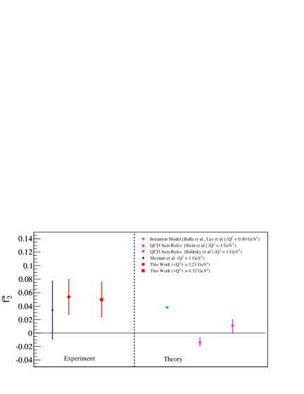
Figure 36: (Color online) Our extracted result for $f_{2}^{n}$ as compared to that from an instanton model Lee et al. (2002); Balla et al. (1998) and QCD sum rules Stein et al. (1995a, b); Balitsky et al. (1990). The result from the analysis of Meziani et al. Meziani et al. (2005) is also shown. For the present data, the inner error bars represent the statistical uncertainties (smaller than the markers), while the outer error bars represent the statistical and systematic uncertainties added in quadrature.

With the matrix elements $d_{2}^{n}$ and $f_{2}^{n}$ evaluated, the Lorentz color force was decomposed into its electric and magnetic components via Burkardt (2013):

$$F_{E}^{y,n}=-\frac{M_{n}^{2}}{6}\left(2d_{2}^{n}+f_{2}^{n}\right)$$ (48)

$$F_{B}^{y,n}=-\frac{M_{n}^{2}}{6}\left(4d_{2}^{n}-f_{2}^{n}\right),$$ (49)

The results for the electric $\left(F_{E}^{y,n}\right)$ and magnetic $\left(F_{B}^{y,n}\right)$ color forces averaged over the volume of the neutron are shown in Table 13 and in Fig. 37, where we compare to an instanton model Lee et al. (2002); Balla et al. (1998) and QCD sum rules from Stein et al. Stein et al. (1995a, b) and Balitsky et al. Balitsky et al. (1990). In the figure, filled markers represent $F_{E}^{y,n}$, while open markers indicate $F_{B}^{y,n}$. We find that the electric and magnetic color forces are approximately equal and opposite. The electric color force component $F_{E}^{y,n}$ is in agreement with the instanton model, while the magnetic component $F_{B}^{y,n}$ is consistent with the instanton model and QCD sum rules. However, those calculations were performed at $Q^{2}=0.4$ and 1 GeV${}^{\text{2}}$, respectively. Note that the values for $F_{E}^{y,n}$ and $F_{B}^{y,n}$ reported here differ from those presented in Ref. Posik et al. (2014) because we have re-evaluated the color forces using the updated $f_{2}^{n}$ values given in Table 12. The central values for $F_{E}^{y,n}$ at $E=4.74$ GeV ($E=5.89$ GeV) have increased in magnitude by 28% (25%), while for $F_{B}^{y,n}$ the central values have increased in magnitude by 16% (24%). The systematic uncertainties for both $F_{E}^{y,n}$ and $F_{B}^{y,n}$ have been reduced by a factor of 1.5.

Table 13: Extracted magnetic and electric Lorentz color force components. The uncertainties given are the statistical and systematic uncertainty, respectively.

$\left<Q^{2}\right>$ $\left(\text{GeV}^{2}\right)$	$F_{E}^{y,n}$ $\left(\text{MeV}/\text{fm}\right)$	$F_{B}^{y,n}$ $\left(\text{MeV}/\text{fm}\right)$
3.21	$-33.53\pm 1.32\pm 19.07$	$52.35\pm 2.43\pm 19.18$
4.32	$-36.48\pm 1.38\pm 19.38$	$38.04\pm 2.55\pm 19.46$

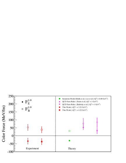
Figure 37: (Color online) Our extracted result for $F_{E}^{y,n}$ (filled markers) and $F_{B}^{y,n}$ (open markers) as compared to an instanton model Lee et al. (2002); Balla et al. (1998) and QCD sum rules Stein et al. (1995a, b); Balitsky et al. (1990). For our data points, the inner error bars represent the statistical uncertainties (smaller than the markers), while the outer error bars represent the statistical and systematic uncertainties added in quadrature.

V.2.4 The virtual photon-nucleon asymmetry $A_{1}^{n}$

The asymmetry $A_{1}^{n}$ (Section IV.4) was extracted for our DIS data at the two beam energies for $\left<Q^{2}\right>=2.59$ GeV² ($E=4.74$ GeV) and $\left<Q^{2}\right>=3.67$ GeV² ($E=5.89$ GeV); the results are given in Tables 14 and 15. These results were averaged using the statistical uncertainty as the weight, while the systematic uncertainties were averaged using equal weights. The averaged results, first published in Parno et al. (2015), are given in Table 16 and plotted in Fig. 38. The systematic uncertainties are outlined in tables given in Appendix E.6. The biggest contribution to the uncertainty is from the effective proton polarization. Our result is consistent with the trend seen in current DIS data from SLAC E142 Anthony et al. (1996) and E154 Abe et al. (1997b), HERMES Ackerstaff et al. (1997) and JLab E99-117 Zheng et al. (2004b, a). Although this experiment was optimized for the measurement of $d_{2}^{n}$, we obtained a data set with uncertainties that are competitive with the previous JLab data from E99-117. Our extraction provides a proof-of-principle measurement in an open-geometry detector (BigBite) yielding data with competitive uncertainties compared to the majority of the world data in the mid-$x$ range, and showing a zero-crossing at $x\approx 0.5$. Our data tend to follow the trend of the pQCD-based parameterization that includes orbital angular momentum Avakian et al. (2007), possibly indicating the importance of orbital angular momentum in the spin of the nucleon. Our result also shows good agreement with the NJL-type model from Cloët et al. Cloët et al. (2005). Dyson-Schwinger Equation treatment predictions Roberts et al. (2013) are presented at $x=1$ (Fig. 38).

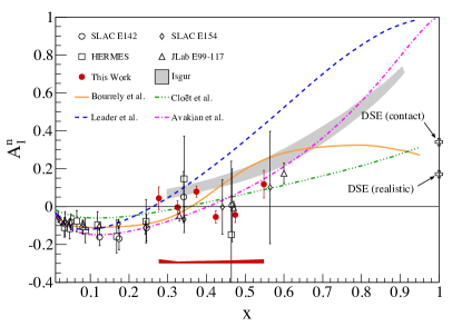
Figure 38: (Color online) Our measured $A_{1}^{n}$ results compared to world data Anthony et al. (1996); Abe et al. (1997a); Zheng et al. (2004b, a); Ackerstaff et al. (1997) and a pQCD-inspired global analysis (dashed) Leader et al. (1998), a statistical quark model (solid) Bourrely and Soffer (2015), a relativistic CQM model (gray band) Isgur (1999) and a pQCD-based parameterization including orbital angular momentum (dash-dotted) Avakian et al. (2007). An NJL-type model (dash triple-dotted) is also shown Cloët et al. (2005). Dyson-Schwinger Equation treatment predictions Roberts et al. (2013) are presented at $x=1$. The band at the bottom of the plot indicates the systematic uncertainty for the present data.

Table 14: Results for $A_{1}^{n}$ and $g_{1}^{n}/F_{1}^{n}$ for $E=4.74$ GeV. The uncertainties given are the statistical and systematic uncertainties, respectively.

$\left<x\right>$	$A_{1}^{n}$	$g_{1}^{n}/F_{1}^{n}$
0.277	$0.012\pm 0.071\pm 0.008$	$0.007\pm 0.068\pm 0.010$
0.325	$0.011\pm 0.043\pm 0.009$	$0.008\pm 0.041\pm 0.008$
0.374	$0.102\pm 0.037\pm 0.014$	$0.065\pm 0.034\pm 0.011$
0.424	$-0.064\pm 0.040\pm 0.014$	$-0.066\pm 0.038\pm 0.013$
0.473	$-0.044\pm 0.051\pm 0.015$	$-0.058\pm 0.047\pm 0.014$

Table 15: Results for $A_{1}^{n}$ and $g_{1}^{n}/F_{1}^{n}$ for $E=5.89$ GeV. The uncertainties given are the statistical and systematic uncertainties, respectively.

$\left<x\right>$	$A_{1}^{n}$	$g_{1}^{n}/F_{1}^{n}$
0.277	$0.127\pm 0.116\pm 0.035$	$0.143\pm 0.112\pm 0.014$
0.325	$-0.031\pm 0.058\pm 0.009$	$-0.019\pm 0.056\pm 0.009$
0.374	$0.035\pm 0.049\pm 0.010$	$0.031\pm 0.046\pm 0.009$
0.424	$-0.039\pm 0.053\pm 0.013$	$-0.049\pm 0.050\pm 0.012$
0.474	$-0.044\pm 0.066\pm 0.017$	$-0.044\pm 0.062\pm 0.015$
0.524	$0.109\pm 0.088\pm 0.019$	$0.098\pm 0.082\pm 0.017$
0.573	$0.135\pm 0.126\pm 0.023$	$0.132\pm 0.116\pm 0.021$

Table 16: Results for $A_{1}^{n}$ and $g_{1}^{n}/F_{1}^{n}$ averaged over our $E=4.74$ and $5.89$ GeV results for $\left<Q^{2}\right>=3.08$ GeV². The uncertainties given are the statistical and systematic uncertainties, respectively.

$\left<x\right>$	$A_{1}^{n}$	$g_{1}^{n}/F_{1}^{n}$
0.277	$0.043\pm 0.060\pm 0.022$	$0.044\pm 0.058\pm 0.012$
0.325	$-0.004\pm 0.035\pm 0.009$	$-0.002\pm 0.033\pm 0.009$
0.374	$0.078\pm 0.029\pm 0.012$	$0.053\pm 0.028\pm 0.010$
0.424	$-0.055\pm 0.032\pm 0.014$	$-0.060\pm 0.030\pm 0.012$
0.474	$-0.044\pm 0.040\pm 0.016$	$-0.053\pm 0.037\pm 0.015$
0.548	$0.118\pm 0.072\pm 0.021$	$0.110\pm 0.067\pm 0.019$

V.2.5 The structure function ratio $g_{1}^{n}/F_{1}^{n}$

Similar to the $A_{1}^{n}$ analysis (Section V.2.4), the $g_{1}^{n}/F_{1}^{n}$ ratio was extracted for our DIS data at each beam energy for $\left<Q^{2}\right>=2.59$ GeV² ($E=4.74$ GeV) and $\left<Q^{2}\right>=3.67$ GeV² ($E=5.89$ GeV). These data are given in Tables 14 and 15. The results were averaged using the statistical uncertainty as the weight, and systematic uncertainties were averaged using equal weights. The averaged results, first published in Parno et al. (2015), are given in Table 16 and plotted in Fig. 39. The systematic uncertainties are given in tables presented in Appendix E.6. The biggest contribution to the uncertainty is from the effective proton polarization and from $A_{1}^{p}$. Our results are comparable to the JLab E99-117 data Zheng et al. (2004b, a) in reach and precision, and are consistent with the trend seen in the DIS data from SLAC E143 Anthony et al. (1996) and E155 Anthony et al. (2000) as shown in Fig. 39.

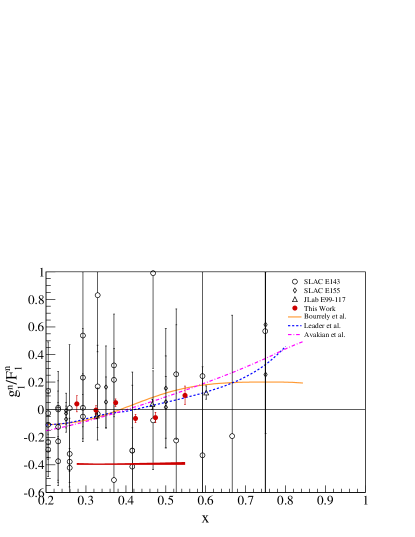
Figure 39: (Color online) Our measured $g_{1}^{n}/F_{1}^{n}$ results, compared to world data Anthony et al. (1996); Abe et al. (1997b); Zheng et al. (2004b, a) and an NLO QCD global analysis Leader et al. (2007) (dashed) and pQCD-inspired fit Avakian et al. (2007) (dash-dotted), and a statistical quark model Bourrely et al. (2002); *Bourrely:2007if (solid). The band at the bottom of the plot indicates the systematic uncertainty for our data set.

V.3 Flavor decomposition via the quark-parton model

Under the quark-parton model Feynman (1969), if one assumes that the strange quark distributions $s(x)$, $\bar{s}(x)$, $\Delta s(x)$ and $\Delta\bar{s}(x)$ are negligible for $x>0.3$, and neglecting any $Q^{2}$-dependence in the ratio of structure functions, the polarized-to-unpolarized quark ratios were extracted through Eqs. I.3 and I.3. We utilized the $R^{du}$ ratio from the CJ12 Owens et al. (2013) model. Using our fit to the $g_{1}^{p}/F_{1}^{p}$ world data sets, we obtained at leading order the quantities $\left(\Delta u+\Delta\bar{u}\right)/\left(u+\bar{u}\right)$ and $\left(\Delta d+\Delta\bar{d}\right)/\left(d+\bar{d}\right)$ for $E=4.74$ GeV (5.89 GeV) where $\left<Q^{2}\right>=2.59$ GeV² (3.67 GeV²). The results are tabulated in Tables 17 and 18. Averaging the two data sets, we obtained the values given in Table 19 at $\left<Q^{2}\right>=3.08$ GeV². These averaged results, first published in Parno et al. (2015), are compared to various world data Zheng et al. (2004a); Dharmawardane et al. (2006); Alekseev et al. (2010a); Airapetian et al. (2005) and theoretical calculations Avakian et al. (2007); Leader et al. (2007); Roberts et al. (2013); Bourrely and Soffer (2015) in Fig. 40. The uncertainty due to neglecting the strange contribution was determined by computing Eqs. I.3 and I.3 with the strange component included Flay (2014):

$$\frac{\Delta u+\Delta\bar{u}}{u+\bar{u}} = \left(\frac{\Delta u+\Delta\bar{u}}{u+\bar{u}}\right)_{s,\bar{s}=0}$$ (50)

$$+ \frac{s+\bar{s}}{u}\left[\frac{4}{15}\frac{g_{1}^{p}}{F_{1}^{p}}-\frac{1}{15}\frac{g_{1}^{n}}{F_{1}^{n}}-\frac{1}{5}\frac{\Delta s+\Delta\bar{s}}{s+\bar{s}}\right]$$

$$\frac{\Delta d+\Delta\bar{d}}{d+\bar{d}} = \left(\frac{\Delta u+\Delta\bar{u}}{u+\bar{u}}\right)_{s,\bar{s}=0}$$ (51)

$$+ \frac{s+\bar{s}}{d}\left[\frac{4}{15}\frac{g_{1}^{n}}{F_{1}^{n}}-\frac{1}{15}\frac{g_{1}^{n}}{F_{1}^{n}}-\frac{1}{5}\frac{\Delta s+\Delta\bar{s}}{s+\bar{s}}\right],$$

where the terms $(\ldots)_{s,\bar{s}=0}$ are defined in Eqs. I.3 and I.3. The second term in Eqs. 50 and 51 is the strange contribution, which was evaluated using various parameterizations de Florian et al. (2005); Leader et al. (2007); de Florian et al. (2008); Bourrely et al. (2002, 2007); Owens et al. (2013) and taking the maximum difference between calculations using all possible model combinations as the uncertainty. It was found to be sizable in the lowest $x$-bins for the down-quark results, but was small for $x\geq 0.424$. For the up-quark results, the strange uncertainty was small. The uncertainty due to neglecting the strange contribution is included in our reported uncertainties.

The extracted up-and down-quark ratios agree with the general trend of the world data within our uncertainties. Our analysis supports the notion that the down-quark ratio stays negative into the large $x$ region, with no clear indication that it turns positive towards $x\simeq 0.6$, as predicted by the Avakian et al. calculation Avakian et al. (2007).

The largest contribution to our systematic uncertainties on the up-quark ratio is from our fit to the $g_{1}^{p}/F_{1}^{p}$ data, while for the down-quark ratio, the largest contributions are due to the $g_{1}^{p}/F_{1}^{p}$ fit and the $d/u$ ratio. An overview of the systematic uncertainties is given in Appendix E.7.

Table 17: Results for $(\Delta u+\Delta\bar{u})/(u+\bar{u})$ and $(\Delta d+\Delta\bar{d})/(d+\bar{d})$ at $E=4.74$ GeV. The uncertainties given are the statistical and systematic uncertainties, respectively.

$\left<x\right>$	$(\Delta u+\Delta\bar{u})/(u+\bar{u})$	$(\Delta d+\Delta\bar{d})/(d+\bar{d})$
0.277	$0.437\pm 0.013\pm 0.031$	$-0.219\pm 0.110\pm 0.028$
0.325	$0.482\pm 0.008\pm 0.036$	$-0.267\pm 0.069\pm 0.032$
0.374	$0.513\pm 0.006\pm 0.043$	$-0.218\pm 0.060\pm 0.038$
0.424	$0.570\pm 0.006\pm 0.050$	$-0.508\pm 0.068\pm 0.051$
0.473	$0.596\pm 0.007\pm 0.063$	$-0.566\pm 0.088\pm 0.069$

Table 18: Results for $(\Delta u+\Delta\bar{u})/(u+\bar{u})$ and $(\Delta d+\Delta\bar{d})/(d+\bar{d})$ at $E=5.89$ GeV. The uncertainties given are the statistical and systematic uncertainties, respectively.

$\left<x\right>$	$(\Delta u+\Delta\bar{u})/(u+\bar{u})$	$(\Delta d+\Delta\bar{d})/(d+\bar{d})$
0.277	$0.410\pm 0.022\pm 0.032$	$0.001\pm 0.182\pm 0.027$
0.325	$0.487\pm 0.010\pm 0.037$	$-0.314\pm 0.094\pm 0.033$
0.374	$0.518\pm 0.008\pm 0.045$	$-0.281\pm 0.081\pm 0.040$
0.424	$0.567\pm 0.008\pm 0.051$	$-0.482\pm 0.090\pm 0.051$
0.474	$0.593\pm 0.009\pm 0.063$	$-0.547\pm 0.116\pm 0.071$
0.524	$0.594\pm 0.012\pm 0.070$	$-0.352\pm 0.165\pm 0.083$
0.573	$0.606\pm 0.015\pm 0.085$	$-0.365\pm 0.250\pm 0.111$

Table 19: Results for $(\Delta u+\Delta\bar{u})/(u+\bar{u})$ and $(\Delta d+\Delta\bar{d})/(d+\bar{d})$ averaged over the two beam energies, for $\left<Q^{2}\right>=3.08$ GeV². The uncertainties given are the statistical and systematic uncertainties, respectively.

$\left<x\right>$	$(\Delta u+\Delta\bar{u})/(u+\bar{u})$	$(\Delta d+\Delta\bar{d})/(d+\bar{d})$
0.277	$0.430\pm 0.011\pm 0.031$	$-0.160\pm 0.094\pm 0.028$
0.325	$0.484\pm 0.006\pm 0.037$	$-0.283\pm 0.055\pm 0.032$
0.374	$0.515\pm 0.005\pm 0.044$	$-0.241\pm 0.048\pm 0.039$
0.424	$0.569\pm 0.005\pm 0.051$	$-0.499\pm 0.054\pm 0.051$
0.474	$0.595\pm 0.006\pm 0.063$	$-0.559\pm 0.070\pm 0.070$
0.548	$0.598\pm 0.009\pm 0.077$	$-0.356\pm 0.138\pm 0.097$

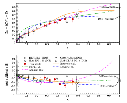
Figure 40: (Color online) Our combined $E=4.74$ and $5.89$ GeV data for the up and down quark ratios. Our results are compared to existing data Zheng et al. (2004a); Dharmawardane et al. (2006); Alekseev et al. (2010a); Airapetian et al. (2005), where the error bars on all data sets are the in-quadrature sum of the statistical and systematic uncertainties. Also presented is a statistical quark model (solid) Bourrely and Soffer (2015), an NLO QCD global analysis from Leader et al. (dashed) Leader et al. (2007), and a pQCD analysis including orbital angular momentum from Avakian et al. (dash-dotted) Avakian et al. (2007). An NJL-type model from Cloët et al. (dash triple-dotted) Cloët et al. (2005) is also shown. DSE predictions Roberts et al. (2013) are shown at $x=1$.

VI Conclusions

Scattering a longitudinally-polarized electron beam of energies of $E=4.74$ GeV and $5.89$ GeV from a polarized ³He target in two orientations, longitudinal and transverse (with respect to the electron beam momentum), we measured the unpolarized electron-scattering cross section with the LHRS and the electron double-spin asymmetries with the BigBite spectrometer, with both spectrometers set at 45^∘ with respect to the beamline. Combining the unpolarized cross sections and double-spin asymmetries allowed the extraction of the twist-3 matrix element $d_{2}^{n}$. This quantity was extracted at two $\left<Q^{2}\right>$ values of 3.21 GeV² and 4.32 GeV². The result at the lower $\left<Q^{2}\right>$ value is small and negative, while that for the higher $\left<Q^{2}\right>$ value is consistent with zero. The data indicate a trend towards the Lattice QCD Göckeler et al. (2005) calculation at $Q^{2}=5$ GeV². The extracted $d_{2}^{n}$ values are also consistent with predictions of chiral soliton Weigel et al. (1997); *Weigel:2000gx and bag Song (1996); Stratmann (1993); Ji and Unrau (1994) models. The size of the present $d_{2}^{n}$ results predicts the twist-3 contribution is small.

Utilizing our measured $d_{2}^{n}$ twist-3 matrix element combined with global analyses for $a_{2}^{n}$ and world data on $\Gamma_{1}^{n}$, we have extracted the twist-4 matrix element $f_{2}^{n}$. This matrix element is observed to be larger than $d_{2}^{n}$ in magnitude, resulting in approximately equal and opposite Lorentz color magnetic and electric forces in the neutron. The results for $f_{2}^{n}$ are consistent with instanton model calculations Balla et al. (1998); Lee et al. (2002) and a QCD sum rule calculation Stein et al. (1995a). The extracted values for $F_{E}^{y,n}$ and $F_{B}^{y,n}$ are in agreement with the instanton model calculations of Balla et al. (1998); Lee et al. (2002), while the value for $F_{B}^{y,n}$ is additionally in accordance with QCD sum-rule calculations from Stein et al. (1995a); Balitsky et al. (1990). We look forward to Lattice QCD calculations of the $f_{2}^{n}$ matrix element, not yet available at this time due to their difficulty, before the new wave of planned experiments in the 12 GeV upgrade era of Jefferson Lab to measure $d_{2}$ and $f_{2}$ with more precision.

Following a similar analysis procedure to the one used for $d_{2}^{n}$, we extracted the $a_{2}^{n}$ matrix element using our $g_{1}^{{}^{3}\text{He}}$ data. Our $a_{2}$ results are positive for both $\left<Q^{2}\right>=3.21$ and $4.32$ GeV², with an improved precision compared to the currently published data and lattice calculations.

The extracted virtual photon asymmetry $A_{1}^{n}$ is consistent with the current world data, especially JLab E99-117 Zheng et al. (2004b, a), and shows good agreement with pQCD calculations that incorporate quark orbital angular momentum Avakian et al. (2007). This suggests that orbital angular momentum may play an important role in the spin of the nucleon.

The measured structure function ratio of $g_{1}^{n}/F_{1}^{n}$ shows a similar trend to JLab E99-117 Zheng et al. (2004b, a), adding higher precision data to the world data set.

Fitting the world $g_{1}/F_{1}$ data on the proton allowed the extraction of $(\Delta u+\Delta\bar{u})/(u+\bar{u})$ and $(\Delta d+\Delta\bar{d})/(d+\bar{d})$ when using the CJ12 Owens et al. (2013) model for $d/u$. The extracted up-quark ratio is consistent with existing measurements and models, and its uncertainty is dominated by our fit to the world $g_{1}^{p}/F_{1}^{p}$ data. The down-quark ratio is observed to remain negative into the large-$x$ region, with no clear indication of a change to positive values in the range of $x\simeq 0.75$ as predicted in Ref. Avakian et al. (2007). The down-quark ratio is very sensitive to the $d/u$ ratio, as is evident in the systematic errors. Better precision on $d/u$ from the projected experiment Petratos et al. (2010) at Jefferson Lab in the 12 GeV upgrade era will help to constrain the $(\Delta d+\Delta\bar{d})/(d+\bar{d})$ ratio.

A future experiment Camsonne et al. (2006) proposed at Jefferson Lab calls for an even higher precision measurement of $d_{2}^{n}$ at four central $Q^{2}$-bins in a range from 2 GeV² to 7 GeV². While our data provide a good understanding of $d_{2}^{n}$ at $Q^{2}=3.21$ and $4.32$ GeV², those data will provide a direct comparison to the Lattice QCD calculation at $Q^{2}=5$ GeV². There are also two dedicated $A_{1}^{n}$ experiments approved to run at Jefferson Lab Averett et al. (2006); Cates et al. (2010) that aim to extend DIS $A_{1}^{n}$ measurements to larger $x$ ($\sim 0.77$) in addition to studying the $Q^{2}$-evolution of the asymmetry. These measurements are important for broadening our insight in the large-$x$ spin structure of the nucleon, as suggested by the results presented in this paper.

Appendix A Deep inelastic electron scattering formalism

A.1 Structure functions and cross sections

In electron scattering, the electrons are accelerated to high energies and scatter from a nuclear or nucleon target. In practice, the target is typically fixed. The electron interacts with the target by exchanging a virtual photon with the target object, transferring its energy and momentum to the target. An advantage of lepton scattering is that the interaction at the leptonic vertex is solely described by quantum electrodynamics, which simplifies the mathematics. The electromagnetic nature of the interaction also results in the process being a “clean” probe into the structure of the nucleon, where the QCD physics is contained entirely in the description of the nucleon and is not convoluted with the leptonic probe.

To describe the process more quantitatively, consider Fig. 41. The incident and scattered electrons have the four-momenta $k=(E,\vec{k})$ and $k^{\prime}=(E^{\prime},\vec{k}^{\prime})$, respectively. The target has a four-momentum of $p=(E_{T},\vec{p})$. The virtual photon exchanged between the incident electron and the target has the four-momentum $q=(\nu,\vec{q})$. If the incident electron has enough energy, the target can break up into a number of distinct hadrons; otherwise, the target will remain intact. In the latter case, the recoiling target object would have a four-momentum $p^{\prime}$ in the final hadronic state. Electron scattering data are presented and discussed in terms of a number of Lorentz-invariant variables, namely $\nu$, $y$, $Q^{2}$, $W$ and $x$. Since the four-momentum at each vertex is conserved, we begin by defining $q$ in terms of the incoming and outgoing electron four-momenta:

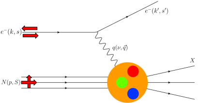
Figure 41: (Color online) A cartoon describing inclusive polarized electron-nucleon scattering. The large arrows indicate possible spin orientations of the incident electron and nucleon. The quantities $s$ and $S$ indicate the spin four-vectors of the electron and nucleon, respectively. The other kinematic variables are described in the text.

$$q=k-k^{\prime}=(E-E^{\prime},\vec{k}-\vec{k}^{\prime})=(\nu,\vec{q}),$$ (52)

where $\nu$ can be defined in an invariant form:

$$\nu\equiv p\cdot q/M,$$ (53)

with $M$ being the mass of the nucleon. In the target rest frame, $p=(M,\vec{0})$, so Eq. 53 reduces to $\nu=E-E^{\prime}$, and is known as the electron energy loss. The fractional energy loss, $y$, can be defined in an invariant form:

$$y\equiv\frac{p\cdot q}{q\cdot k},$$ (54)

which simplifies to the non-invariant form $y=(E-E^{\prime})/E$.

The four-momentum transfer squared, $q^{2}$, always evaluates to less than or equal to zero. For convenience, we define a positive quantity $Q^{2}$:

$$Q^{2}\equiv-q^{2}=4EE^{\prime}\sin^{2}\left(\theta/2\right),$$ (55)

where $\theta$ is the scattering angle of the electron in the laboratory frame and we have neglected the electron mass.

Shifting our focus to the hadronic side of Fig. 41, there are two possibilities for the final state: there is one object (i.e., the target remains intact) or several, determined by the energy with which the target is probed. Furthermore, the measured interaction may be described by two general terms: exclusive or inclusive scattering. In the case of exclusive scattering, the scattered electron and all final-state hadrons are detected; there is also the case of detecting an electron and at least one particle in the final state, which is called semi-inclusive. For inclusive scattering, only the scattered electron is detected in the final state.

Inclusive scattering can be represented as $eN\rightarrow eX$, where $e$ is the electron, $N$ is the target nucleon and $X$ is the final (unmeasured) hadronic state. In the context of an unmeasured final hadronic state (which could consist of any of the multitude of particle states for a given combination of $\nu$ and $Q^{2}$ values), we can define the invariant mass of the system, $W$:

$$W^{2}\equiv\left(q+p\right)^{2}=M^{2}+2M\nu-Q^{2}.$$ (56)

Finally, we come to the variable $x$. It is defined in terms of the other invariants $\nu$ and $Q^{2}$ as:

$$x\equiv\frac{Q^{2}}{2p\cdot q}=\frac{Q^{2}}{2M\nu}.$$ (57)

The simplest interpretation of $x$ comes in the infinite momentum frame, where the nucleon is traveling with a large momentum along $\vec{q}$. In this frame, the active quark in the interaction (struck by the virtual photon) carries the momentum fraction $x$ of the nucleon momentum in the leading-order DIS process Halzen and Martin (1984).

The DIS region is characterized by $W>2$ GeV, where $\nu$ and $Q^{2}$ become large enough so that the quarks can be resolved inside the nucleon. In this case, the electron is scattering from an asymptotically free quark (or anti-quark) in the nucleon.

Consider scattering unpolarized electrons from pointlike, unpolarized spin-1/2 particles that are infinitely heavy with a charge of $+1$. In this case, energy conservation dictates $E^{\prime}=E$ and the cross section is given by:

$$\left(\frac{d\sigma}{d\Omega}\right)_{\text{Mott}}=\frac{\alpha^{2}\cos^{2}\left(\theta/2\right)}{4E^{2}\sin^{4}\left(\theta/2\right)},$$ (58)

with $\theta$ being the scattering angle of the electron. This quantity is known as the Mott cross section. However, since the nucleon is a composite object and is not infinitely massive, the cross section is more complicated than that seen in Eq. 58, and is given by:

$$\frac{d^{2}\sigma^{\text{unpol.}}}{d\Omega dE^{\prime}} = \left(\frac{d\sigma}{d\Omega}\right)_{\text{Mott}}\Bigg{[}\frac{1}{\nu}F_{2}\left(x,Q^{2}\right)$$ (59)

$$+ \frac{2\tan^{2}\left(\theta/2\right)}{M}F_{1}\left(x,Q^{2}\right)\Bigg{]},$$

where $F_{1}$ and $F_{2}$ are the unpolarized structure functions, and are related to one another through Eq. 43.

For experiments that use targets that are not nucleons ($A\neq 1$), there are two conventions for expressing the quantities $F_{1}$ and $F_{2}$. The first is per nucleon, written as $F_{1}/A$ and $F_{2}/A$. The second is per nucleus, where the structure functions are reported without dividing by $A$. The latter representation is used in this paper.

When both the incident electron beam and target are polarized, one can access the spin structure functions $g_{1}$ and $g_{2}$. A full discussion may be found in Ref. Anselmino et al. (1995). The polarized cross section difference for when the target spin (double arrows) and electron spin (single arrows) are polarized along the direction of the electron momentum is given as:

$$\frac{d^{2}\sigma^{\downarrow,\Uparrow}}{d\Omega dE^{\prime}}-\frac{d^{2}\sigma^{\uparrow,\Uparrow}}{d\Omega dE^{\prime}} = \frac{4\alpha^{2}}{Q^{2}}\frac{E^{\prime}}{\nu E}\big{[}\left(E+E^{\prime}\cos\theta\right)g_{1}\left(x,Q^{2}\right)$$ (60)

$$- 2Mxg_{2}\left(x,Q^{2}\right)\big{]}.$$

When the target spin is perpendicular to the electron spin, the cross section difference is written as:

$$\frac{d^{2}\sigma^{\downarrow,\Rightarrow}}{d\Omega dE^{\prime}}-\frac{d^{2}\sigma^{\uparrow,\Rightarrow}}{d\Omega dE^{\prime}} = \frac{4\alpha^{2}}{Q^{2}}\frac{E^{\prime 2}}{\nu E}\sin\theta\big{[}g_{1}\left(x,Q^{2}\right)$$ (61)

$$+ \frac{2ME}{\nu}g_{2}\left(x,Q^{2}\right)\big{]}.$$

A.2 Bjorken scaling, the quark-parton model and scaling violation

When probing an object of finite size, the measurement will depend upon the spatial resolution of the probe; in the case of electron scattering, this is $Q^{2}$, the negative of the momentum transferred to the target squared. If we increase $Q^{2}$ so that we can resolve the internal structure of the nucleon, the quarks will become visible. At this point, inelastic electron-nucleon scattering may be seen as elastic scattering from a single quark, while the other quarks remain undisturbed. Considering that quarks are pointlike particles, increasing the resolution $Q^{2}$ will no longer affect the interaction.

In the limit where $Q^{2}$ $\rightarrow\infty$ and $\nu\rightarrow\infty$, with $x=Q^{2}/(2M\nu)$ fixed (the Bjorken limit), the phenomenon where experimental observables lose their $Q^{2}$-dependence is known as Bjorken scaling Bjorken and Paschos (1969). As a result, the structure functions depend upon a single variable $x$. Furthermore, the $F_{2}$ structure function can be related to the $F_{1}$ structure function by the Callan-Gross relation Callan and Gross (1969):

$$F_{2}(x)=2xF_{1}(x).$$ (62)

To connect the quark behavior to the structure functions, we turn to the quark-parton model (QPM). In this model, deep inelastic scattering of electrons from nucleons is described as the incoherent scattering of electrons from free partons (quarks and anti-quarks) inside the nucleon Feynman (1969), via the exchange of a virtual photon. Therefore, the nucleon structure functions $F_{1}$ and $g_{1}$ can be written in terms of the parton distribution functions (PDFs) Feynman (1969); Halzen and Martin (1984):

$$F_{1}\left(x\right) = \frac{1}{2}\sum_{i}e_{i}^{2}q_{i}\left(x\right)$$ (63)

$$g_{1}\left(x\right) = \frac{1}{2}\sum_{i}e_{i}^{2}\Delta q_{i}\left(x\right),$$ (64)

with $q=q^{\uparrow}(x)+q^{\downarrow}(x)$ and $\Delta q=q^{\uparrow}(x)-q^{\downarrow}(x)$, where $\uparrow$ ($\downarrow$) indicates quark spin parallel (antiparallel) to the parent nucleon spin.

The scaling behavior of the structure functions is only exact in the limit of infinite $Q^{2}$ and $\nu$. At finite values of $Q^{2}$ and $\nu$, it is only an approximation. In reality, the quarks participating in the interaction with the electron may radiate gluons before or after scattering. Such processes result in an infinite cross section, and can only be treated properly when all other processes of the same order are considered. These gluonic radiative corrections result in the cross section acquiring a logarithmic $Q^{2}$ dependence, which can be computed exactly in pQCD under the formalism of the Dokshitzer-Gribov-Lipatov-Altarelli-Parisi (DGLAP) evolution equations Dokshitzer (1977); *Gribov:1972ri; *Altarelli:1977zs. As a result, the $Q^{2}$-dependence manifests itself in the structure functions.

As a result of the scaling violation, we re-cast the PDFs and the structure functions in terms of both $x$ and $Q^{2}$. In particular, the definition of the PDF is now $q^{\uparrow(\downarrow)}(x,Q^{2})$: this is the probability of finding a quark $q$ with its spin parallel (antiparallel) to its parent nucleon with momentum fraction $x$ when viewed at an energy scale $Q=\sqrt{Q^{2}}$.

The physical interpretation tied to scaling violation is that structure functions at low $Q^{2}$ are dominated by three valence quarks “dressed” by sea quarks (manifesting as $q$-$\bar{q}$ pairs) and gluons. As $Q^{2}$ is increased, the resolving power increases, allowing for sensitivity to the “bare” quarks and gluons which make up the nucleon.

A.3 The resonance region

Due to the kinematics of our experiment, about half of our data set corresponds to the DIS regime, while the other corresponds to the resonance region. With this in mind, we give a brief description of the resonance region.

When $\nu$ and $Q^{2}$ have values such that $1.2<W<2$ GeV, we explore the substructure of the nucleon. In this energy range, the quarks that make up the nucleon collectively absorb the energy of the virtual photon, leading to unstable excited states of the nucleon called nucleon resonances. The most prominent resonance occurs at $W=1.232$ GeV, and is known as the $\Delta$ resonance. Higher resonances are also possible at $W>1.4$ GeV, but are difficult to discern from one another, as their peaks and tails tend to overlap.

A.4 The virtual photon-nucleon asymmetry $A_{1}$

Let us consider a scattering interaction in which the nucleon is longitudinally polarized, while the virtual photon is circularly polarized with a helicity of $\pm 1$. As a result, two possible helicity-dependent cross sections for a given nucleon polarization arise, denoted $\sigma_{3/2}$ and $\sigma_{1/2}$. The subscripts denote the projection of the total spin of the virtual photon-nucleon system along the direction of the virtual photon momentum Abe et al. (1998); Zheng (2002). When the virtual photon spin is parallel (antiparallel) to the nucleon spin, they add to 3/2 (1/2). From these two cross sections, the $A_{1}$ asymmetry is formed as:

$$A_{1}\equiv\frac{\sigma_{1/2}-\sigma_{3/2}}{\sigma_{1/2}+\sigma_{3/2}}.$$ (65)

In terms of the structure functions, $A_{1}$ may be written as Anselmino et al. (1995):

$$A_{1}\left(x,Q^{2}\right)=\frac{g_{1}\left(x,Q^{2}\right)-\gamma^{2}g_{2}\left(x,Q^{2}\right)}{F_{1}\left(x,Q^{2}\right)}.$$ (66)

At large $Q^{2}$, $A_{1}\approx g_{1}/F_{1}$. This can be seen by observing that $\gamma^{2}\rightarrow 0$ as $Q^{2}$ gets increasingly large. A conceptual argument on the quark level is as follows: if the spin of the virtual photon is antiparallel to that of the quark, then the virtual photon can be absorbed and the quark spin is flipped; however, if the spins are parallel, then the absorption of the virtual photon is forbidden, since the total projection of the spins along $\vec{q}$ is 3/2 and the quark is a spin-1/2 particle. The mathematical form of the approximation can be illustrated using this physical interpretation: for the case where the spins of the nucleon and virtual photon are parallel ($\sigma_{3/2}$), then the quark that can absorb the virtual photon has its spin antiparallel to the nucleon spin. This translates to: $\sigma_{3/2}\sim\sum\limits_{i}e_{i}^{2}q_{i}^{\downarrow}(x)$. A similar argument may be made for the $\sigma_{1/2}$ case where only quarks with spins parallel to the parent nucleon can absorb virtual photons. Thus, we have: $\sigma_{1/2}\sim\sum\limits_{i}e_{i}^{2}q_{i}^{\uparrow}(x)$. Rewriting $A_{1}$ in terms of these approximations, we obtain:

$$A_{1}\sim\frac{\sum\limits_{i}e_{i}^{2}\left[q_{i}^{\uparrow}(x)-q_{i}^{\downarrow}(x)\right]}{\sum\limits_{i}e_{i}^{2}\left[q_{i}^{\uparrow}(x)+q_{i}^{\downarrow}(x)\right]}=\frac{\sum\limits_{i}e_{i}^{2}\Delta q_{i}(x)}{\sum\limits_{i}e_{i}^{2}q_{i}(x)}=\frac{g_{1}(x)}{F_{1}(x)},$$ (67)

where the last term arises from the quark-parton model description of the $F_{1}$ and $g_{1}$ structure functions (Eqs. 63 and 64).

The $A_{1}$ asymmetry is a ratio of structure functions ($\approx g_{1}/F_{1}$), and as a result there is very little $Q^{2}$ dependence. This is because $g_{1}$ and $F_{1}$ follow the same $Q^{2}$ evolution described by the DGLAP equations Dokshitzer (1977); *Gribov:1972ri; *Altarelli:1977zs which tends to cancel in the ratio, leading to $A_{1}$ being roughly $Q^{2}$-independent.

A.5 Electron asymmetries

The virtual photon-nucleon asymmetry $A_{1}$ is defined in terms of a ratio of the difference in virtual photon cross sections to their sum. Due to the difficulty associated with aligning the virtual photon spin along the direction of the nucleon spin, another approach is utilized to measure $A_{1}$ that consists of aligning the incident electron spin relative to the direction of the nucleon spin. The extraction of the electron asymmetries allows the determination of $A_{1}$. After some algebra, the electron asymmetries (Section I.2) may be written as Melnitchouk et al. (2005):

$$A_{\parallel} = D\left(A_{1}+\eta A_{2}\right)$$ (68)

$$A_{\perp} = d\left(A_{2}-\eta A_{1}\right).$$ (69)

The asymmetry $A_{2}$ is defined as $A_{2}\equiv 2\sigma_{LT}/\left(\sigma_{1/2}+\sigma_{3/2}\right)$, where $\sigma_{LT}$ is the cross section describing the interference between virtual photons with longitudinal and transverse polarizations. In the QPM, there is no clear interpretation for $\sigma_{LT}$, and in turn $A_{2}$, as there is for $\sigma_{1/2}$, $\sigma_{3/2}$ and $A_{1}$ Drechsel et al. (2001). From Eqs. 68 and 69, one can write $A_{1}$ and $A_{2}$ in terms of the double-spin asymmetries $A_{\parallel}$ and $A_{\perp}$. Similar equations may be obtained for $g_{1}/F_{1}$ and $g_{2}/F_{1}$ Melnitchouk et al. (2005). The equations for $A_{1}$ and $g_{1}/F_{1}$ are shown in Section I.3.

A.6 Spin structure functions

The spin structure functions $g_{1}$ and $g_{2}$ may be obtained from the measured unpolarized cross section $\sigma_{0}$ and the double-spin asymmetries $A_{\parallel}$ and $A_{\perp}$ through:

$$g_{1} = \frac{MQ^{2}}{4{\alpha}^{2}}\frac{2y}{\left(1-y\right)\left(2-y\right)}\sigma_{0}\Big{[}A_{\parallel}$$

$$+\tan\left(\theta/2\right)A_{\perp}\Big{]}$$

$$g_{2} = \frac{MQ^{2}}{4{\alpha}^{2}}\frac{y^{2}}{\left(1-y\right)\left(2-y\right)}\sigma_{0}\times$$

$$\left[-A_{\parallel}+\frac{1+\left(1-y\right)\cos\theta}{\left(1-y\right)\sin\theta}A_{\perp}\right].$$

Appendix B Quark-gluon correlations

B.1 The operator product expansion and twist

The operator product expansion (OPE) allows the separation of the perturbative and non-perturbative components in structure functions at finite $Q^{2}$. This concept is illustrated in the product of two local quark (or gluon) operators $\mathcal{O}_{a}(d)\mathcal{O}_{b}$ separated by a distance $d$ in the limit of $d\rightarrow 0$:

$$\lim_{d\rightarrow 0}\mathcal{O}_{a}(d)\mathcal{O}_{b}(0)=\sum\limits_{k}c_{abk}(d)\mathcal{O}_{k}(0),$$ (72)

where the coefficient functions $c_{abk}$ are the Wilson coefficients and contain the perturbative part, which can be computed using perturbation theory since non-perturbative effects occur at distances much larger than $d$ Manohar (1992). The non-perturbative components manifest in $\mathcal{O}_{k}(0)$, and contribute to the cross section on the order of $x^{-n}(Q/M)^{D-2-n}$. The exponents $n$ and $D$ are the spin and (mass) dimension of the operator, respectively. The quantity $Q=\sqrt{Q^{2}}$. The twist $\tau$ of the operator is defined by:

$$\tau\equiv D-n.$$ (73)

At large $Q^{2}$, $\tau=2$ terms dominate in the OPE; at low $Q^{2}$, higher-twist $(\tau>2)$ operators become important.

B.2 Cornwall-Norton moments and Nachtmann moments

Using the OPE, an infinite set of sum rules may be derived under a twist expansion of the spin structure functions $g_{1}$ and $g_{2}$ Anselmino et al. (1995). Such expansions of $g_{1}$ and $g_{2}$ are known as the Cornwall-Norton (CN) moments Melnitchouk et al. (2005):

$$\int_{0}^{1}x^{n-1}g_{1}\left(x,Q^{2}\right)dx = \frac{1}{2}a_{n-1},\text{ }n=1,3,5,\ldots$$ (74)

$$\int_{0}^{1}x^{n-1}g_{2}\left(x,Q^{2}\right)dx = \frac{n-1}{2n}\left(d_{n-1}-a_{n-1}\right),$$

$$n=3,5,7,\ldots,$$

where $n$ indicates the $n^{\text{th}}$ moment. In Eqs 74 and B.2, only twist-2 and twist-3 contributions are considered. The quantities $a_{n-1}$ and $d_{n-1}$ represent the twist-2 and twist-3 matrix elements, respectively . The expansions are only over odd integers, which is a result of the symmetry of the structure functions under charge conjugation Slifer (2004).

The twist-3 matrix elements $d_{n-1}$ may be accessed by combining Eqs. 74 and B.2. One obtains Melnitchouk et al. (2005):

$$\int_{0}^{1}x^{n-1}\left[g_{1}\left(x,Q^{2}\right)+\frac{n}{n-1}g_{2}\left(x,Q^{2}\right)\right]dx=\frac{d_{n-1}}{2},\quad n\geq 3.$$ (76)

Choosing $n=3$ yields the equation for $d_{2}$ (cf. Eq. 4).

The study of higher twist in structure functions has traditionally been done through the formalism of the CN moments; however, the exact relation of the CN moments to the dynamical higher-twist contributions has come into question in recent analyses Melnitchouk et al. (2005); Dong (2008). It is argued that the CN moments are only valid when the terms connected to the finite mass of the nucleon are neglected. Such terms are known as target mass corrections. These corrections are related to twist-2 operators, and are of order $\mathcal{O}(M^{2}/Q^{2})$. Analogous to the CN moments, the Nachtmann moments $M_{1}$ and $M_{2}$ can be used to separate the higher-twist contribution from the target mass corrections Nachtmann (1973); Wandzura (1977); Georgi and Politzer (1976); Matsuda and Uematsu (1980); Sidorov and Stamenov (2006); Accardi and Melnitchouk (2008). They are defined as Melnitchouk et al. (2005); Piccione and Ridolfi (1998); Slifer et al. (2010):

$$M_{1}^{n}\left(Q^{2}\right) \equiv \frac{1}{2}a_{n-1}=\frac{1}{2}\tilde{a}_{n}E_{1}^{n}$$

$$= \int_{0}^{1}\frac{\xi^{n+1}}{x^{2}}\Bigg{[}\frac{x}{\xi}-\frac{n^{2}}{(n+2)^{2}}\frac{M^{2}x\xi}{Q^{2}}g_{1}\left(x,Q^{2}\right)$$

$$- \frac{4n}{n+2}\frac{M^{2}x^{2}}{Q^{2}}g_{2}\left(x,Q^{2}\right)\Bigg{]}dx,$$

$$n=1,3,\ldots$$

$$M_{2}^{n}\left(Q^{2}\right) \equiv \frac{1}{2}d_{n-1}=\frac{1}{2}\tilde{d}_{n}E_{2}^{n}$$

$$= \int_{0}^{1}\frac{\xi^{n+1}}{x^{2}}\Bigg{[}\frac{x}{\xi}g_{1}\left(x,Q^{2}\right)$$

$$+ \left(\frac{n}{n-1}\frac{x^{2}}{\xi^{2}}-\frac{n}{n+1}\frac{M^{2}x^{2}}{Q^{2}}\right)g_{2}\left(x,Q^{2}\right)\Bigg{]}dx,$$

$$n=3,5,\ldots.$$

We have performed the analysis to extract $d_{2}^{n}$ according to the CN moments, and checked that result against what was obtained from using the Nachtmann moments. The difference in results between the two approaches was found to be negligible, on the order of $10^{-5}$ in absolute value.

Appendix C Fits to data

C.1 Cross section fits

As discussed in Section IV.2, due to time constraints not all cross section measurements for studying pair production on ³He and N₂ were carried out. To resolve the absence of those data, the data that were collected were fit to a function of the form:

$$f\left(E_{p}\right)=\frac{1}{E_{p}^{2}}e^{\left(a_{0}+a_{1}E_{p}\right)},$$ (79)

where the scattered electron energy $E_{p}$ is in GeV. This was done for $\sigma^{e^{+}}$, $\sigma_{\text{N}_{2}}^{e^{-}}$ and $\sigma_{\text{N}}^{e^{+}}$. The fits were performed in ROOT ROO , and the extracted parameters and their uncertainties were obtained from the Minuit minimization package James and Roos (1975). The fits were done separately for the data sets corresponding to each beam energy. The systematic uncertainties on the fits was obtained by varying the parameters within their errors and observing the change on the fit (see Figs 18 and 19). The parameters together with their uncertainties are listed in Table 20 for the nitrogen cross section when scattered electrons were detected, $\sigma_{\text{N}_{\text{2}}}^{e^{-}}$ (LHRS set to negative polarity mode), and in Table 21 when positrons were detected, $\sigma_{\text{N}_{\text{2}}}^{e^{+}}$ (LHRS in positive polarity mode). Table 22 gives the fit parameters and their uncertainties for the unpolarized ³He cross section where positrons were detected, $\sigma^{e^{+}}$ (LHRS in positive polarity mode).

Table 20: Fit parameters for the nitrogen cross section (negative polarity), $\sigma_{\text{N}_{\text{2}}}^{e^{-}}$, for $E=4.74$ GeV and $E=5.89$ GeV.

Par.	$E=4.74$ GeV	$E=5.89$ GeV
$a_{0}$	$1.465\text{E+}01\pm 4.919\text{E-}02$	$1.480\text{E+}01\pm 5.647\text{E-}02$
$a_{1}$	$-1.825\text{E-}03\pm 4.770\text{E-}05$	$-2.123\text{E-}03\pm 5.607\text{E-}05$

Table 21: Fit parameters for the nitrogen cross section (positive polarity), $\sigma_{\text{N}_{\text{2}}}^{e^{+}}$, for $E=4.74$ GeV and $E=5.89$ GeV.

Par.	$E=4.74$ GeV	$E=5.89$ GeV
$a_{0}$	$1.559\text{E+}01\pm 1.604\text{E-}01$	$1.614\text{E+}01\pm 2.120\text{E-}01$
$a_{1}$	$-4.699\text{E-}03\pm 2.255\text{E-}04$	$-5.232\text{E-}03\pm 3.126\text{E-}04$

Table 22: Fit parameters for the positron cross section on ³He, $\sigma^{e^{+}}$, for $E=4.74$ GeV and $E=5.89$ GeV.

Par.	$E=4.74$ GeV	$E=5.89$ GeV
$a_{0}$	$1.887\text{E+}01\pm 7.998\text{E-}02$	$1.896\text{E+}01\pm 6.899\text{E-}02$
$a_{1}$	$-5.620\text{E-}03\pm 1.194\text{E-}04$	$-5.421\text{E-}03\pm 9.286\text{E-}05$

C.2 $g_{1}^{p}/F_{1}^{p}$ fit

To carry out the analysis to obtain $g_{1}^{n}/F_{1}^{n}$ from our $g_{1}^{{}^{3}\text{He}}/F_{1}^{{}^{3}\text{He}}$ data, a parameterization of the $g_{1}^{p}/F_{1}^{p}$ data was needed. We fit the world data to a three-parameter, $Q^{2}$-independent function given by:

$$f(x)=p_{0}+p_{1}x+p_{2}x^{2}.$$ (80)

The assumption of $Q^{2}$-independence is reasonable as the $Q^{2}$-evolution in $g_{1}$ and $F_{1}$ partially cancels in the ratio to leading order and next-to-leading order in $Q^{2}$ Anselmino et al. (1995). Additionally, the world data (which are at differing $Q^{2}$) show roughly the same behavior. The world data considered were from HERMES Ackerstaff et al. (1997), SLAC E143 Abe et al. (1998) and E155 Anthony et al. (1999), along with CLAS EG1b Dharmawardane et al. (2006) and CLAS EG1-DVCS Prok et al. (2014). First, all of these data were rebinned in $x$, in new bins formed based on a statistical-error-weighted average; the systematic errors of all data contributing to a new bin were averaged with equal weights to yield its systematic error. The fit result, with $\chi^{2}/\text{ndf}=0.91$, is shown in Fig. 42 The fit parameters were found to be:

$$p_{0} = 0.035\pm 0.008$$

$$p_{1} = 1.478\pm 0.077$$ (81)

$$p_{2} = -1.010\pm 0.138.$$

The fit was performed in ROOT ROO , and the extracted parameters and their uncertainties were obtained from the Minuit minimization package James and Roos (1975). The band indicates the uncertainty on the fit which was taken as the spread in the $g_{1}^{p}/F_{1}^{p}$ data, serving as a conservative estimate.

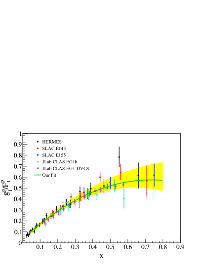
Figure 42: (Color online) Our fit to world $g_{1}^{p}/F_{1}^{p}$ data. The error bars on the data are the in-quadrature sums of their statistical and systematic uncertainties. The band indicates the error on the fit.

C.3 $A_{1}^{p}$ fit

To obtain $A_{1}^{n}$ from our $A_{1}^{{}^{3}\text{He}}$ data, we followed a similar procedure to the $g_{1}/F_{1}$ analysis. The data used in the fit include measurements from SMC Adeva et al. (1998), HERMES Airapetian et al. (2007), EMC Ashman et al. (1988, 1989), SLAC E143 Abe et al. (1998) and E155 Anthony et al. (1999), COMPASS Alekseev et al. (2010b) and CLAS EG1b Dharmawardane et al. (2006). The fit is shown in Fig. 43, where we obtained $\chi^{2}/\text{ndf}=1.11$. The fit parameters were found to be:

$$p_{0} = 0.044\pm 0.007$$

$$p_{1} = 1.423\pm 0.078$$ (82)

$$p_{2} = -0.552\pm 0.158.$$

The fit was performed in ROOT ROO , and the extracted parameters and their uncertainties were obtained from the Minuit minimization package James and Roos (1975). The band in Fig. 43 gives the fit uncertainty, computed in the same fashion as was done for the $g_{1}^{p}/F_{1}^{p}$ fit.

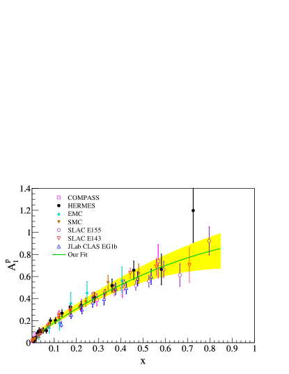
Figure 43: (Color online) Our fit to world $A_{1}^{p}$ data. The error bars on the data are the in-quadrature sums of their statistical and systematic uncertainties. The band indicates the uncertainty on the fit.

Appendix D World $\Gamma_{1}^{n}$ Data

The world $\Gamma_{1}^{n}$ data from SLAC E142 Anthony et al. (1996), E143 Abe et al. (1998) and E154 Abe et al. (1997b), SMC Adeva et al. (1998), HERMES Airapetian et al. (2003), and JLab RSS Slifer et al. (2010) and E94-010 Slifer et al. (2008) used in our $f_{2}^{n}$ analysis are shown in Fig. 44. The twist-2 contribution, $\mu_{2}^{n}$, given by the solid curve; its uncertainty is indicated by the band. The elastic contribution is also shown, given as the dashed curve. For more details, see Section V.2.3.

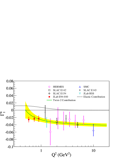
Figure 44: (Color online) $\Gamma_{1}^{n}$ for the world data from SLAC E142 Anthony et al. (1996), E143 Abe et al. (1998) and E154 Abe et al. (1997b), SMC Adeva et al. (1998), HERMES Airapetian et al. (2003), and JLab RSS Slifer et al. (2010) and E94-010 Slifer et al. (2008). The uncertainties on the world data are the in-quadrature sum of statistical and systematic uncertainties. The elastic contribution is given by the dashed curve, and has been added to the data. The twist-2 contribution is indicated by the solid curve and its uncertainty is given by the band, which is dominated by the uncertainty in $\alpha_{s}$.

Subtracting $\mu_{2}^{n}$ from $\Gamma_{1}^{n}$ yields the higher-twist contribution, $\Delta\Gamma_{1}^{n}\equiv\Gamma_{1}^{n}-\mu_{2}^{n}$, shown in Fig. 45. Fitting these data to the function

$$f\left(\frac{1}{Q^{2}}\right)=\frac{A}{Q^{2}}+\frac{B}{Q^{4}}$$ (83)

where $A=\left(M_{n}^{2}/9\right)\left(a_{2}^{n}+4d_{2}^{n}+4f_{2}^{n}\right)$ and $B=\mu_{6}$, a higher-twist ($\tau>4$) term, are free parameters. Using the result for the fit parameter $A$, we extract $f_{2}^{n}$ after inserting the average $a_{2}^{n}$ from global analyses and our measured $d_{2}^{n}$ (see Section V.2.3) into Eq. 83. The values of the fit parameters $A$ and $B$ were found to be:

$$A = 1.936\text{E-}2$$

$$B = -1.675\text{E-}2,$$ (84)

with the error matrix:

$$\varepsilon=\left(\begin{array}[]{c c}2.240\text{E-}4&-1.653\text{E-}4\\ -1.653\text{E-}4&1.351\text{E-}4\end{array}\right).$$ (85)

The fit was performed in ROOT ROO , and the extracted parameters and their uncertainties were obtained from the Minuit minimization package James and Roos (1975). This fit allowed the extraction of $f_{2}^{n}$ as described in Section V.2.3.

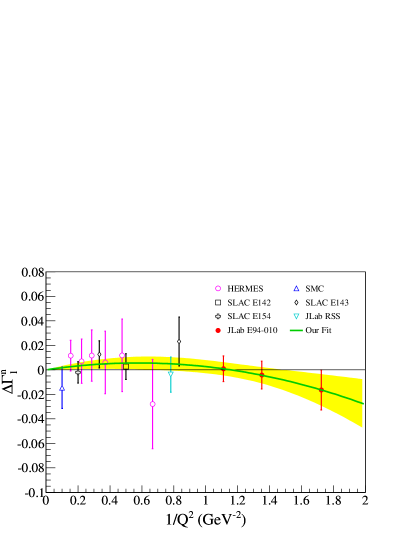
Figure 45: (Color online) $\Delta\Gamma_{1}^{n}\equiv\Gamma_{1}^{n}-\mu_{2}^{n}$ for the world data shown in Fig. 44. The uncertainties on the world data are the in-quadrature sum of statistical and systematic uncertainties. Our fit is indicated by the solid curve and its uncertainty is given by the yellow band.

Appendix E Systematic Uncertainty Tables

This section contains tables of showing the contributing factors to the systematic uncertainties for the final unpolarized cross sections and double-spin asymmetries, $d_{2}^{n}$, $g_{1}^{{}^{3}\text{He}}$, $g_{2}^{{}^{3}\text{He}}$, $A_{1}^{{}^{3}\text{He}}$, $A_{1}^{n}$, $g_{1}^{{}^{3}\text{He}}/F_{1}^{{}^{3}\text{He}}$, $g_{1}^{n}/F_{1}^{n}$ and the flavor-separated ratios $(\Delta u+\Delta\bar{u})/(u+\bar{u})$ and $(\Delta d+\Delta\bar{d})/(d+\bar{d})$.

E.1 Final unpolarized cross section systematic uncertainties

The breakdown of the systematic uncertainty on the unpolarized cross sections is given in Tables 23 and 24. The column “Cuts” indicates uncertainties due to event cuts, which includes the gas Čerenkov, $E/p$, and target cuts to remove the target windows; “Background” corresponds to uncertainties related to the positron and nitrogen background subtractions; “Misc.” refers to the uncertainties incurred from the beam charge calibration, and the density of nitrogen and ³He in the target cell; “RC” is the uncertainty due to the radiative corrections, as explained in Section IV.2.3. The final column (“Total”) gives the in-quadrature sum of all uncertainties in the row.

Table 23: Systematic uncertainty breakdown for the unpolarized ³He cross section at E = 4.74 GeV. All uncertainties are in nb/GeV/sr. See Appendix E.1 for a discussion of the various contributions to the systematic uncertainty.

$<x>$	Cuts	Background	Misc.	RC	Total
0.214	1.700E-01	3.800E-01	2.440E-01	2.870E-01	5.610E-01
0.299	1.390E-01	1.170E-01	2.120E-01	2.400E-02	2.810E-01
0.456	6.400E-02	1.700E-02	1.000E-01	5.000E-03	1.210E-01
0.494	5.300E-02	1.200E-02	8.800E-02	1.000E-03	1.030E-01
0.533	4.700E-02	8.000E-03	7.000E-02	0.000E+00	8.400E-02
0.579	3.600E-02	6.000E-03	5.300E-02	2.000E-03	6.500E-02
0.629	2.800E-02	4.000E-03	4.000E-02	4.000E-03	5.000E-02
0.686	2.000E-02	3.000E-03	2.800E-02	5.000E-03	3.500E-02
0.745	1.500E-02	3.000E-03	2.100E-02	9.000E-03	2.800E-02

Table 24: Systematic uncertainty breakdown for the unpolarized ³He cross section at E = 5.89 GeV. All uncertainties are in nb/GeV/sr. See Appendix E.1 for a discussion of the various contributions to the systematic uncertainty.

$<x>$	Cuts	Background	Misc.	RC	Total
0.208	1.060E-01	3.710E-01	1.610E-01	2.600E-01	4.920E-01
0.247	1.120E-01	2.280E-01	1.710E-01	4.700E-02	3.100E-01
0.330	5.600E-02	6.100E-02	9.800E-02	1.700E-02	1.300E-01
0.434	4.400E-02	1.700E-02	6.300E-02	4.000E-03	7.900E-02
0.468	3.800E-02	1.100E-02	4.900E-02	4.000E-03	6.300E-02
0.503	2.900E-02	8.000E-03	4.200E-02	1.000E-03	5.200E-02
0.539	2.600E-02	6.000E-03	3.300E-02	0.000E+00	4.200E-02
0.580	1.800E-02	4.000E-03	2.700E-02	1.000E-03	3.300E-02
0.629	1.100E-02	3.000E-03	1.900E-02	2.000E-03	2.200E-02
0.679	9.000E-03	2.000E-03	1.300E-02	2.000E-03	1.600E-02
0.738	7.000E-03	2.000E-03	1.000E-02	4.000E-03	1.300E-02

E.2 Final asymmetry systematic uncertainties

Tables 25, 28, 27 and 28 list the systematic uncertainties assigned to the double-spin physics asymmetries $A_{\parallel}$ and $A_{\perp}$ on ³He. The systematic uncertainty depends on the electron beam polarization $P_{b}$, the target polarization $P_{b}$, the nitrogen dilution factor $D_{\text{N}_{2}}$, and contaminations in the BigBite analysis due to $\pi^{-}$ ($f_{1}$), $\pi^{+}$ ($f_{2}$), and $e^{+}$ ($f_{3}$). Also there are contributions from the electron selection cuts (“Cuts”) and the radiative corrections (“RC”). The final column (“Total”) is the in-quadrature sum of the uncertainties in each row. Columns for all quantities except for the PID cuts have been omitted since they were very small for the lowest $x$-bins, and were negligible otherwise.

Table 25: Systematic uncertainties assigned to $A_{\parallel}^{{}^{3}\text{He}}$ at an incident beam energy of 4.74 GeV. See Appendix E.2 for a discussion of the various contributions to the systematic uncertainty.

$<x>$	Cuts	Total
0.277	7.000E-03	7.000E-03
0.325	2.000E-03	3.000E-03
0.374	2.000E-03	2.000E-03
0.424	4.000E-03	5.000E-03
0.473	3.000E-03	3.000E-03
0.523	2.000E-03	2.000E-03
0.574	4.000E-03	4.000E-03
0.623	2.000E-03	3.000E-03
0.673	4.000E-03	5.000E-03
0.723	6.000E-03	6.000E-03
0.773	1.300E-02	1.300E-02
0.823	1.100E-02	1.100E-02
0.874	1.700E-02	1.700E-02

Table 26: Systematic uncertainties assigned to $A_{\perp}^{{}^{3}\text{He}}$ at an incident beam energy of 4.74 GeV See Appendix E.2 for a discussion of the various contributions to the systematic uncertainty.

$<x>$	Cuts	Total
0.277	2.000E-03	2.000E-03
0.325	2.000E-03	2.000E-03
0.374	2.000E-03	2.000E-03
0.424	2.000E-03	2.000E-03
0.473	1.000E-03	1.000E-03
0.523	1.000E-03	1.000E-03
0.574	2.000E-03	2.000E-03
0.623	2.000E-03	2.000E-03
0.673	3.000E-03	3.000E-03
0.723	2.000E-03	2.000E-03
0.773	4.000E-03	5.000E-03
0.823	6.000E-03	6.000E-03
0.874	4.000E-03	6.000E-03

Table 27: Systematic uncertainties assigned to $A_{\parallel}^{{}^{3}\text{He}}$ at an incident beam energy of 5.89 GeV See Appendix E.2 for a discussion of the various contributions to the systematic uncertainty.

$<x>$	Cuts	Total
0.277	9.000E-03	1.000E-02
0.325	3.000E-03	3.000E-03
0.374	2.000E-03	2.000E-03
0.424	2.000E-03	3.000E-03
0.474	6.000E-03	6.000E-03
0.524	2.000E-03	2.000E-03
0.573	3.000E-03	3.000E-03
0.624	5.000E-03	5.000E-03
0.674	5.000E-03	5.000E-03
0.723	5.000E-03	5.000E-03
0.773	8.000E-03	8.000E-03
0.823	1.400E-02	1.400E-02
0.873	1.700E-02	1.700E-02

Table 28: Systematic uncertainties assigned to $A_{\perp}^{{}^{3}\text{He}}$ at an incident beam energy of 5.89 GeV See Appendix E.2 for a discussion of the various contributions to the systematic uncertainty.

$<x>$	Cuts	Total
0.277	2.000E-03	3.000E-03
0.325	1.000E-03	1.000E-03
0.374	0.000E+00	0.000E+00
0.424	1.000E-03	1.000E-03
0.474	1.000E-03	1.000E-03
0.524	1.000E-03	1.000E-03
0.573	1.000E-03	1.000E-03
0.624	1.000E-03	1.000E-03
0.674	2.000E-03	2.000E-03
0.723	3.000E-03	3.000E-03
0.773	2.000E-03	2.000E-03
0.823	3.000E-03	4.000E-03
0.873	7.000E-03	7.000E-03

E.3 Polarized spin structure function systematic uncertainties

Tables 29, 31, 30 and 32 list the systematic uncertainties assigned to the polarized spin-structure functions. A number of factors contribute to the systematic uncertainty, including kinematics (“Kin.”) and all of the systematic uncertainties found to contribute to the final asymmetries, namely $P_{b}$, $P_{t}$, $f_{1}$, $f_{2}$ $f_{3}$, PID cuts (“Cuts”) and radiative corrections (“RC”). Other contributions include the systematic uncertainty on the unpolarized cross section ($\sigma_{0}$), in addition to the uncertainties associated with the interpolation or extrapolation of the data where necessary. The value for each these uncertainties was determined by varying each of these contributions within reasonable limits and taking the corresponding change in the observable (either $g_{1}^{{}^{3}\text{He}}$ or $g_{2}^{{}^{3}\text{He}}$) as the uncertainty. The last column (“Total”) is the in-quadrature sum of the uncertainties in each row. All uncertainties are absolute. Columns for all quantities except for the PID cuts have been omitted since they were very small for the lowest $x$-bins, and were negligible otherwise.

Table 29: Systematic uncertainties assigned to $g_{1}^{{}^{3}\text{He}}$ at an incident beam energy of 4.74 GeV See Appendix E.3 for a discussion of the various contributions to the systematic uncertainty.

$<x>$	Cuts	Total
0.277	8.000E-03	9.000E-03
0.325	2.000E-03	2.000E-03
0.374	2.000E-03	2.000E-03
0.424	3.000E-03	3.000E-03
0.473	1.000E-03	2.000E-03
0.523	0.000E+00	0.000E+00
0.574	1.000E-03	1.000E-03
0.623	0.000E+00	1.000E-03
0.673	1.000E-03	1.000E-03
0.723	0.000E+00	1.000E-03
0.773	1.000E-03	1.000E-03
0.823	1.000E-03	1.000E-03
0.874	0.000E+00	1.000E-03

Table 30: Systematic uncertainties assigned to $g_{2}^{{}^{3}\text{He}}$ at an incident beam energy of 4.74 GeV See Appendix E.3 for a discussion of the various contributions to the systematic uncertainty.

$<x>$	Cuts	Total
0.277	9.000E-03	9.000E-03
0.325	6.000E-03	6.000E-03
0.374	4.000E-03	5.000E-03
0.424	2.000E-03	2.000E-03
0.473	0.000E+00	1.000E-03
0.523	1.000E-03	1.000E-03
0.574	1.000E-03	1.000E-03
0.623	1.000E-03	1.000E-03
0.673	1.000E-03	1.000E-03
0.723	0.000E+00	1.000E-03
0.773	0.000E+00	1.000E-03
0.823	0.000E+00	0.000E+00
0.874	0.000E+00	1.000E-03

Table 31: Systematic uncertainties assigned to $g_{1}^{{}^{3}\text{He}}$ at an incident beam energy of 5.89 GeV See Appendix E.3 for a discussion of the various contributions to the systematic uncertainty.

$<x>$	Cuts	Total
0.277	1.000E-02	1.200E-02
0.325	2.000E-03	3.000E-03
0.374	2.000E-03	2.000E-03
0.424	1.000E-03	2.000E-03
0.474	2.000E-03	2.000E-03
0.524	1.000E-03	1.000E-03
0.573	1.000E-03	1.000E-03
0.624	1.000E-03	1.000E-03
0.674	0.000E+00	0.000E+00
0.723	0.000E+00	0.000E+00
0.773	0.000E+00	0.000E+00
0.823	0.000E+00	0.000E+00
0.873	0.000E+00	0.000E+00

Table 32: Systematic uncertainties assigned to $g_{2}^{{}^{3}\text{He}}$ at an incident beam energy of 5.89 GeV See Appendix E.3 for a discussion of the various contributions to the systematic uncertainty.

$<x>$	Cuts	Total
0.277	1.400E-02	1.900E-02
0.325	5.000E-03	6.000E-03
0.374	1.000E-03	2.000E-03
0.424	2.000E-03	2.000E-03
0.474	2.000E-03	2.000E-03
0.524	1.000E-03	1.000E-03
0.573	1.000E-03	1.000E-03
0.624	0.000E+00	0.000E+00
0.674	0.000E+00	0.000E+00
0.723	0.000E+00	0.000E+00
0.773	0.000E+00	0.000E+00
0.823	0.000E+00	1.000E-03
0.873	0.000E+00	0.000E+00

E.4 $d_{2}^{n}$ systematic uncertainties

A breakdown of the $d_{2}^{n}$ systematic uncertainties is given in Table 33, for each of the measured mean $Q^{2}$ points. This table includes the effects of all the uncertainties found in the preceding tables (i.e. $P_{p}$, $P_{t}$, etc.), referred to as experimental systematics (“Exp.”), in addition to radiative corrections, $d_{2}^{p}$, the proton and neutron polarizations ($\tilde{P}_{p}$ and $\tilde{P}_{n}$), and the unmeasured low $x$ contributions. The value for each these uncertainties was determined by varying each of these contributions within reasonable limits and taking the corresponding change in $d_{2}^{n}$ as the uncertainty. The two sources of uncertainty that dominate the $d_{2}^{n}$ systematic uncertainty are those from the experimental and low-$x$ contributions. However, the final $d_{2}^{n}$ measurement’s statistical uncertainty is larger than its systematic uncertainty.

Table 33: Systematic uncertainties assigned to different regions of $d_{2}^{n}$. “Res” indicates the contribution from the resonance region; in particular, from data with $W<2$ GeV. “DIS” represents the contribution due to data for $W>2$ GeV. See Appendix E.4 for a discussion of the various contributions to the systematic uncertainty.

Region	$\left<Q^{2}\right>$ $\left(\text{GeV}^{\text{2}}\right)$	Exp.	RC	$d_{2}^{p}$	$\tilde{P}_{p}$, $\tilde{P}_{n}$ (high error)	$\tilde{P}_{p}$, $\tilde{P}_{n}$ (low error)	Low $x$	Total
DIS+Res	3.21	4.700E-04	2.000E-05	4.000E-05	6.000E-05	1.000E-04	5.800E-04	7.500E-04
DIS+Res	4.32	3.700E-04	2.000E-05	4.000E-05	2.000E-05	4.000E-05	5.800E-04	6.900E-04
DIS	2.59	3.600E-04	1.000E-05	5.000E-05	3.000E-05	5.000E-05	—	3.700E-04
DIS	3.67	2.900E-04	2.000E-05	4.000E-05	2.000E-05	2.000E-05	—	2.900E-04
Res	4.71	2.200E-04	0.000E+00	4.000E-05	3.000E-05	5.000E-05	—	2.300E-04
Res	5.99	1.100E-04	0.000E+00	2.000E-05	1.000E-05	3.000E-05	—	1.200E-04

E.5 $a_{2}$ systematic uncertainties

The systematic uncertainties for the measured $a_{2}^{{}^{3}\text{He}}$ are given in Table 34, where the column labeled $g_{1}^{{}^{3}\text{He}}$ corresponds to the uncertainty due to our $g_{1}^{{}^{3}\text{He}}$ data, and the column labeled $x$ is the uncertainty due to $x$ in the integration. The value of these uncertainties was determined by varying each of these contributions within reasonable limits and taking the change in the $a_{2}^{n}$ as the uncertainty. The in-quadrature sum of the two contributions is given as the column labeled “Total.” The systematic uncertainties for the $a_{2}^{n}$ extraction for the full $x$-range are presented in Table 35. The columns labeled low-$x$ (high-$x$) correspond to the uncertainties due to the low-$x$ (high-$x$) regions. The uncertainty due to the effective proton (neutron) polarization is given by the column labeled $\tilde{P}_{p}$ ($\tilde{P}_{n}$). The uncertainties due to $a_{2}^{p}$ and our measured $a_{2}^{{}^{3}\text{He}}$ are also given.

Table 34: The systematic uncertainties contributing to the $a_{2}^{{}^{3}\text{He}}$ result in the measured $x$-range. See Appendix E.5 for a discussion of the various contributions to the systematic uncertainty.

$\left<Q^{2}\right>$ $\left(\text{GeV}^{\text{2}}\right)$	$g_{1}^{{}^{3}\text{He}}$	$x$	Total
3.21	3.428E-05	8.803E-06	3.539E-05
4.32	3.281E-05	6.681E-06	3.348E-05

Table 35: The systematic uncertainties contributing to the $a_{2}^{n}$ result over the full $x$-range. See Appendix E.5 for a discussion of the various contributions to the systematic uncertainty listed below.

$\left<Q^{2}\right>$ $\left(\text{GeV}^{\text{2}}\right)$	low-$x$	high-$x$	$\tilde{P}_{p}$	$\tilde{P}_{n}$	$a_{2}^{p}$	$a_{2}^{{}^{3}\text{He}}$	Total
3.21	1.374E-4	1.373E-04	2.439E-04	3.012E-04	3.068E-04	3.052E-04	6.125E-04
4.32	8.878E-5	8.880E-05	2.518E-04	3.054E-04	3.118E-04	3.089E-04	6.042E-04

E.6 $A_{1}$ and $g_{1}/F_{1}$ systematic uncertainties

This section discusses the breakdown of the systematic uncertainties on $A_{1}^{{}^{3}\text{He}}$ and $A_{1}^{n}$. The main factors that contribute to the uncertainties on the ³He data are the physics asymmetries $A_{\parallel}$ and $A_{\perp}$, and the kinematic factors $D$, $\eta$, $\xi$ and $d$ (see Section I.3). Each physics asymmetry was varied within its uncertainty, and the change in $A_{1}^{{}^{3}\text{He}}$ was observed. For the kinematics, the low-level variables of the electron momentum $p$ and scattering angle $\theta$ were changed within their relative uncertainties of $1\%$ and $1.4\%$ Flay (2014) respectively, and the kinematic factors were re-evaluated, and the change in the $A_{1}$ asymmetry was observed. The resulting contributions to the systematic uncertainty in $A_{1}^{{}^{3}\text{He}}$ are listed in Tables 36 and 37 for the 4.74 GeV and 5.89 GeV runs, respectively.

The systematic uncertainties for $A_{1}^{n}$ are listed in in Tables 38 and 39. The inputs in the $A_{1}^{n}$ extraction that were varied consisted of $F_{2}^{n}$ and $F_{2}^{p}$, $F_{2}^{{}^{3}\text{He}}$, $A_{1}^{p}$ and our $A_{1}^{{}^{3}\text{He}}$ data. For the neutron and proton $F_{2}$, various models Pumplin et al. (2002); Owens et al. (2013); Bourrely et al. (2002); *Bourrely:2007if were compared, and the largest difference in $A_{1}^{n}$ was taken as the uncertainty, listed in the $F_{2}^{n,p}$ column. The same procedure was used for $F_{2}^{{}^{3}\text{He}}$, where the models considered were F1F209 Bosted and Mamyan (2012) and NMC95 Arneodo et al. (1995). This uncertainty is given in the $F_{2}^{{}^{3}\text{He}}$ column. Our fit of the world $A_{1}^{p}$ data was varied within its uncertainty and the change in $A_{1}^{n}$ was taken as the uncertainty, listed in the $A_{1}^{p}$ column. The values for the effective neutron (proton) polarization $\tilde{P}_{n}$ ($\tilde{P}_{p}$) were varied within their uncertainties, and the change in $A_{1}^{n}$ was taken as the uncertainty. These contributions are listed as $\tilde{P}_{n}$ and $\tilde{P}_{p}$ for the neutron and proton, respectively. We varied our $A_{1}^{{}^{3}\text{He}}$ data within their systematic uncertainties and observed the changes in the $A_{1}^{n}$ results, which were taken as the uncertainties, listed in the $A_{1}^{{}^{3}\text{He}}$ column. The in-quadrature sum of all contributions is given in the column labeled “Total”.

To evaluate the systematic uncertainties on $g_{1}/F_{1}$ data, shown in Tables 40, 41, 42 and 43, the same procedure used for the $A_{1}$ data was applied. The same models for $F_{2}$ on the neutron, proton and ³He were used, in addition to the effective polarizations of the neutron and proton, $\tilde{P}_{n}$ and $\tilde{P}_{p}$.

Table 36: Systematic uncertainties for $A_{1}^{{}^{3}\text{He}}$ data at E = 4.74 GeV. See Appendix E.6 for a discussion of the various contributions to the systematic uncertainty.

$<x>$	$A_{\parallel}$	$A_{\perp}$	Kin.	Total
0.277	3.850E-03	1.900E-04	1.200E-04	3.860E-03
0.325	1.480E-03	1.400E-04	7.000E-05	1.480E-03
0.374	9.900E-04	2.100E-04	5.400E-04	1.150E-03
0.424	2.650E-03	1.700E-04	1.200E-04	2.660E-03
0.473	1.840E-03	1.100E-04	1.900E-04	1.850E-03
0.523	1.100E-03	1.600E-04	1.900E-04	1.130E-03
0.574	2.430E-03	3.300E-04	2.000E-04	2.460E-03
0.623	1.840E-03	3.600E-04	1.400E-04	1.880E-03
0.673	2.620E-03	5.000E-04	1.300E-04	2.670E-03
0.723	3.770E-03	4.400E-04	2.000E-04	3.800E-03
0.773	7.510E-03	8.900E-04	3.900E-04	7.570E-03
0.823	7.000E-03	1.180E-03	3.200E-04	7.100E-03
0.874	1.019E-02	1.250E-03	1.960E-03	1.045E-02

Table 37: Systematic uncertainties for $A_{1}^{{}^{3}\text{He}}$ data at E = 5.89 GeV. See Appendix E.6 for a discussion of the various contributions to the systematic uncertainty.

$<x>$	$A_{\parallel}$	$A_{\perp}$	Kin.	Total
0.277	5.520E-03	1.800E-04	5.900E-04	5.550E-03
0.325	1.850E-03	9.000E-05	2.400E-04	1.870E-03
0.374	1.230E-03	4.000E-05	4.000E-05	1.230E-03
0.424	1.510E-03	1.100E-04	2.200E-04	1.530E-03
0.474	3.270E-03	9.000E-05	4.000E-05	3.270E-03
0.524	1.200E-03	1.200E-04	1.000E-05	1.210E-03
0.573	1.800E-03	1.400E-04	1.300E-04	1.810E-03
0.624	3.120E-03	1.000E-04	1.600E-04	3.130E-03
0.674	2.770E-03	2.700E-04	7.000E-05	2.780E-03
0.723	2.740E-03	3.900E-04	1.300E-04	2.770E-03
0.773	4.430E-03	3.500E-04	1.100E-04	4.450E-03
0.823	7.870E-03	7.100E-04	6.600E-04	7.930E-03
0.873	9.270E-03	1.170E-03	1.400E-04	9.340E-03

Table 38: Systematic uncertainties for $A_{1}^{n}$ at E = 4.74 GeV. See Appendix E.6 for a discussion of the various contributions to the systematic uncertainty.

$<x>$	$F_{2}^{n,p}$	$F_{2}^{{}^{3}\text{He}}$	$\tilde{P}_{p}$	$\tilde{P}_{n}$	$A_{1}^{p}$	$A_{1}^{{}^{3}\text{He}}$	Total
0.277	2.730E-03	7.000E-04	5.160E-03	1.500E-04	5.080E-03	2.680E-03	8.220E-03
0.325	2.690E-03	1.010E-03	6.160E-03	1.200E-04	6.050E-03	1.850E-03	9.280E-03
0.374	6.900E-03	6.500E-04	7.200E-03	1.690E-03	6.690E-03	6.370E-03	1.371E-02
0.424	5.980E-03	1.810E-03	8.310E-03	1.190E-03	7.710E-03	6.390E-03	1.449E-02
0.473	5.740E-03	1.710E-03	9.570E-03	8.500E-04	8.960E-03	5.280E-03	1.537E-02

Table 39: Systematic uncertainties for $A_{1}^{n}$ at E = 5.89 GeV. See Appendix E.6 for a discussion of the various contributions to the systematic uncertainty.

$<x>$	$F_{2}^{n,p}$	$F_{2}^{{}^{3}\text{He}}$	$\tilde{P}_{p}$	$\tilde{P}_{n}$	$A_{1}^{p}$	$A_{1}^{{}^{3}\text{He}}$	Total
0.277	4.500E-03	4.000E-04	5.140E-03	2.070E-03	5.130E-03	3.370E-02	3.483E-02
0.325	2.440E-03	1.310E-03	6.140E-03	5.900E-04	5.810E-03	3.060E-03	9.430E-03
0.374	2.650E-03	6.400E-04	7.190E-03	5.200E-04	6.700E-03	1.470E-03	1.032E-02
0.424	2.900E-03	2.120E-03	8.300E-03	7.400E-04	7.940E-03	3.740E-03	1.263E-02
0.474	3.940E-03	1.350E-03	9.560E-03	8.400E-04	9.240E-03	9.750E-03	1.702E-02
0.524	9.950E-03	0.000E+00	1.096E-02	1.720E-03	1.060E-02	5.050E-03	1.897E-02
0.573	1.300E-02	1.500E-04	1.247E-02	2.140E-03	1.207E-02	8.000E-03	2.321E-02

Table 40: Systematic uncertainties for $g_{1}^{{}^{3}\text{He}}/F_{1}^{{}^{3}\text{He}}$ data at E = 4.74 GeV. See Appendix E.6 for a discussion of the various contributions to the systematic uncertainty.

$<x>$	$A_{\parallel}$	$A_{\perp}$	Kin.	Total
0.277	3.680E-03	5.300E-04	4.000E-05	3.720E-03
0.325	1.340E-03	3.500E-04	4.000E-05	1.380E-03
0.374	9.200E-04	4.900E-04	4.000E-05	1.040E-03
0.424	2.560E-03	3.300E-04	1.300E-04	2.580E-03
0.473	1.710E-03	2.000E-04	1.100E-04	1.720E-03
0.523	1.030E-03	2.600E-04	2.000E-05	1.060E-03
0.574	2.200E-03	4.700E-04	3.000E-05	2.260E-03
0.623	1.610E-03	5.000E-04	1.700E-04	1.690E-03
0.673	2.430E-03	6.700E-04	1.400E-04	2.530E-03
0.723	3.350E-03	5.100E-04	2.000E-04	3.390E-03
0.773	6.410E-03	9.700E-04	1.600E-04	6.490E-03
0.823	5.760E-03	1.260E-03	2.800E-04	5.900E-03
0.874	8.590E-03	1.230E-03	3.200E-04	8.680E-03

Table 41: Systematic uncertainties for $g_{1}^{{}^{3}\text{He}}/F_{1}^{{}^{3}\text{He}}$ data at E = 5.89 GeV. See Appendix E.6 for a discussion of the various contributions to the systematic uncertainty.

$<x>$	$A_{\parallel}$	$A_{\perp}$	Kin.	Total
0.277	5.320E-03	2.570E-03	5.000E-05	5.910E-03
0.325	1.720E-03	1.070E-03	4.000E-05	2.030E-03
0.374	1.170E-03	1.900E-04	1.000E-05	1.190E-03
0.424	1.350E-03	9.500E-04	4.000E-05	1.650E-03
0.474	3.160E-03	1.100E-04	5.000E-05	3.160E-03
0.524	1.200E-03	1.100E-04	0.000E+00	1.200E-03
0.573	1.640E-03	6.800E-04	1.000E-05	1.780E-03
0.624	2.720E-03	9.100E-04	2.000E-05	2.870E-03
0.674	2.420E-03	4.400E-04	1.000E-05	2.460E-03
0.723	2.370E-03	1.070E-03	2.000E-05	2.600E-03
0.773	3.900E-03	1.120E-03	4.000E-05	4.060E-03
0.823	7.090E-03	1.068E-02	1.800E-04	1.282E-02
0.873	8.480E-03	2.030E-03	1.000E-04	8.720E-03

Table 42: Systematic uncertainties for $g_{1}^{n}/F_{1}^{n}$ at E = 4.74 GeV. See Appendix E.6 for a discussion of the various contributions to the systematic uncertainty.

$<x>$	$F_{2}^{n,p}$	$F_{2}^{{}^{3}\text{He}}$	$\tilde{P}_{p}$	$\tilde{P}_{n}$	$g_{1}^{p}/F_{1}^{p}$	$g_{1}^{{}^{3}\text{He}}/F_{1}^{{}^{3}\text{He}}$	Total
0.277	2.530E-03	7.100E-04	5.320E-03	1.200E-04	2.950E-03	7.630E-03	1.011E-02
0.325	2.480E-03	9.800E-04	6.270E-03	1.300E-04	3.650E-03	3.060E-03	8.310E-03
0.374	5.640E-03	2.900E-04	7.230E-03	1.080E-03	4.680E-03	2.470E-03	1.064E-02
0.424	5.770E-03	1.730E-03	8.190E-03	1.100E-03	6.020E-03	6.360E-03	1.346E-02
0.473	6.020E-03	1.700E-03	9.240E-03	9.700E-04	7.600E-03	5.050E-03	1.445E-02

Table 43: Systematic uncertainties for $g_{1}^{n}/F_{1}^{n}$ at E = 5.89 GeV. See Appendix E.6 for a discussion of the various contributions to the systematic uncertainty.

$<x>$	$F_{2}^{n,p}$	$F_{2}^{{}^{3}\text{He}}$	$\tilde{P}_{p}$	$\tilde{P}_{n}$	$g_{1}^{p}/F_{1}^{p}$	$g_{1}^{{}^{3}\text{He}}/F_{1}^{{}^{3}\text{He}}$	Total
0.277	4.500E-03	4.500E-04	5.100E-03	2.450E-03	2.970E-03	1.193E-02	1.427E-02
0.325	2.180E-03	1.160E-03	6.030E-03	3.300E-04	3.760E-03	4.510E-03	8.780E-03
0.374	2.420E-03	6.200E-04	6.950E-03	5.300E-04	4.790E-03	2.920E-03	9.290E-03
0.424	3.110E-03	2.110E-03	7.890E-03	8.400E-04	6.020E-03	4.410E-03	1.152E-02
0.474	3.770E-03	1.260E-03	8.900E-03	7.600E-04	7.280E-03	9.170E-03	1.525E-02
0.524	9.150E-03	0.000E+00	9.980E-03	1.680E-03	9.620E-03	3.940E-03	1.716E-02
0.573	1.240E-02	1.500E-04	1.111E-02	2.280E-03	1.183E-02	7.140E-03	2.176E-02

E.7 Flavor decomposition systematic uncertainties

Tables 44 and 45 give a breakdown of the systematic uncertainties at $E=4.74$ GeV for the up and down quark ratios, respectively. Tables 46 and 47 list the uncertainties for $E=5.89$ GeV. The columns of the table represent the contribution due to our $g_{1}^{n}/F_{1}^{n}$ data, our fit to world $g_{1}^{p}/F_{1}^{p}$ data, the $(d+\bar{d})/(u+\bar{u})$ parameterization, and the strange uncertainty, respectively. The value of these uncertainties, except for the strange uncertainty (see Section V.3), was determined by varying each of these contributions within reasonable limits and taking the change in the quark ratio as the uncertainty. This was done for both the up and down quark ratios. The in-quadrature sum of all contributions is displayed in the last column, labeled “Total.”

Table 44: Systematic uncertainties for $(\Delta u+\Delta\bar{u})/(u+\bar{u})$ at $E=4.74$ GeV. See Appendix E.7 for a discussion of the various contributions to the systematic uncertainty.

$<x>$	$g_{1}^{n}/F_{1}^{n}$	$g_{1}^{p}/F_{1}^{p}$	$(d+\bar{d})/(u+\bar{u})$	$s$	Total
0.277	9.900E-04	2.918E-02	3.260E-03	8.700E-03	3.064E-02
0.325	7.800E-04	3.556E-02	3.590E-03	6.450E-03	3.633E-02
0.374	9.300E-04	4.243E-02	3.610E-03	4.580E-03	4.284E-02
0.424	1.090E-03	4.967E-02	4.620E-03	3.280E-03	5.000E-02
0.473	1.100E-03	6.300E-02	5.070E-03	2.350E-03	6.326E-02

Table 45: Systematic uncertainties for $(\Delta d+\Delta\bar{d})/(d+\bar{d})$ at $E=4.74$ GeV. See Appendix E.7 for a discussion of the various contributions to the systematic uncertainty.

$<x>$	$g_{1}^{n}/F_{1}^{n}$	$g_{1}^{p}/F_{1}^{p}$	$(d+\bar{d})/(u+\bar{u})$	$s$	Total
0.277	8.240E-03	1.518E-02	1.455E-02	1.673E-02	2.811E-02
0.325	7.140E-03	2.027E-02	1.886E-02	1.363E-02	3.167E-02
0.374	9.290E-03	2.647E-02	2.280E-02	1.071E-02	3.770E-02
0.424	1.193E-02	3.399E-02	3.467E-02	8.140E-03	5.066E-02
0.473	1.343E-02	4.814E-02	4.754E-02	5.940E-03	6.923E-02

Table 46: Systematic uncertainties for $(\Delta u+\Delta\bar{u})/(u+\bar{u})$ at $E=5.89$ GeV. See Appendix E.7 for a discussion of the various contributions to the systematic uncertainty.

$<x>$	$g_{1}^{n}/F_{1}^{n}$	$g_{1}^{p}/F_{1}^{p}$	$(d+\bar{d})/(u+\bar{u})$	$s$	Total
0.277	1.380E-03	3.088E-02	1.980E-03	8.300E-03	3.207E-02
0.325	8.100E-04	3.675E-02	3.750E-03	6.190E-03	3.746E-02
0.374	7.800E-04	4.430E-02	3.800E-03	4.390E-03	4.469E-02
0.424	9.400E-04	5.109E-02	4.460E-03	3.110E-03	5.139E-02
0.474	1.160E-03	6.267E-02	4.810E-03	2.220E-03	6.290E-02
0.524	1.220E-03	6.976E-02	4.130E-03	1.600E-03	6.991E-02
0.573	1.430E-03	8.454E-02	3.860E-03	1.240E-03	8.465E-02

Table 47: Systematic uncertainties for $(\Delta d+\Delta\bar{d})/(d+\bar{d})$ at $E=5.89$ GeV. See Appendix E.7 for a discussion of the various contributions to the systematic uncertainty.

$<x>$	$g_{1}^{n}/F_{1}^{n}$	$g_{1}^{p}/F_{1}^{p}$	$(d+\bar{d})/(u+\bar{u})$	$s$	Total
0.277	1.158E-02	1.622E-02	8.640E-03	1.631E-02	2.716E-02
0.325	7.470E-03	2.116E-02	1.973E-02	1.339E-02	3.274E-02
0.374	7.850E-03	2.792E-02	2.503E-02	1.036E-02	3.969E-02
0.424	1.039E-02	3.539E-02	3.438E-02	7.810E-03	5.102E-02
0.474	1.436E-02	4.863E-02	4.929E-02	5.660E-03	7.094E-02
0.524	1.731E-02	6.181E-02	5.298E-02	3.580E-03	8.331E-02
0.573	2.341E-02	8.633E-02	6.641E-02	2.130E-03	1.114E-01

References

- Mcallister and Hofstadter (1956) R. W. Mcallister and R. Hofstadter, Phys. Rev. 102, 851 (1956).
- Bloom et al. (1969) E. D. Bloom et al., Phys. Rev. Lett. 23, 930 (1969).
- Breidenbach et al. (1969) M. Breidenbach et al., Phys. Rev. Lett. 23, 935 (1969).
- Gross and Wilczek (1973a) D. J. Gross and F. Wilczek, Phys. Rev. Lett. 30, 1343 (1973a).
- Gross and Wilczek (1973b) D. Gross and F. Wilczek, Phys. Rev. D 8, 3633 (1973b).
- Gross and Wilczek (1974) D. Gross and F. Wilczek, Phys. Rev. D 9, 980 (1974).
- Kuhn et al. (2009) S. Kuhn, J.-P. Chen, and E. Leader, Prog. Part. Nucl. Phys. 63, 1 (2009), arXiv:0812.3535 [hep-ph] .
- Aidala et al. (2013) C. A. Aidala, S. D. Bass, D. Hasch, and G. K. Mallot, Rev. Mod. Phys. 85, 655 (2013).
- Adare et al. (2014) A. Adare et al. (PHENIX), Phys. Rev. D 90, 012007 (2014), arXiv:1402.6296 [hep-ex] .
- Adamczyk et al. (2015) L. Adamczyk et al. (STAR), Phys. Rev. Lett. 115, 092002 (2015), arXiv:1405.5134 [hep-ex] .
- Shuryak and Vainshtein (1982a) E. V. Shuryak and A. I. Vainshtein, Nucl. Phys. B 201, 141 (1982a).
- Jaffe (1990) R. Jaffe, Comments Nucl. Part. Phys. 19, 239 (1990).
- Jaffe and Ji (1991) R. L. Jaffe and X.-D. Ji, Phys. Rev. D 43, 724 (1991).
- Dokshitzer (1977) Y. L. Dokshitzer, Sov. Phys. JETP 46, 641 (1977).
- Gribov and Lipatov (1972) V. Gribov and L. Lipatov, Sov. J. Nucl. Phys. 15, 438 (1972).
- Altarelli and Parisi (1977) G. Altarelli and G. Parisi, Nucl. Phys. B 126, 298 (1977).
- Bjorken (1966) J. D. Bjorken, Phys. Rev. 148, 1467 (1966).
- Bjorken (1970) J. D. Bjorken, Phys. Rev. D 1, 1376 (1970).
- Manohar (1992) A. V. Manohar, (1992), arXiv:hep-ph/9204208 [hep-ph] .
- Cortes et al. (1992) J. L. Cortes, B. Pire, and J. Ralston, Z. Phys. C 55, 409 (1992).
- Filippone and Ji (2001) B. W. Filippone and X.-D. Ji, Adv. Nucl. Phys. 26, 1 (2001), arXiv:hep-ph/0101224 [hep-ph] .
- Wandzura and Wilczek (1977) S. Wandzura and F. Wilczek, Phys. Lett. B 72, 195 (1977).
- Wilson (1969) K. G. Wilson, Phys. Rev. 179, 1499 (1969).
- Ehrnsperger et al. (1994) B. Ehrnsperger, A. Schäfer, and L. Mankiewicz, Phys. Lett. B 323, 439 (1994), arXiv:hep-ph/9311285 [hep-ph] .
- Burkardt (2013) M. Burkardt, Phys. Rev. D 88, 114502 (2013).
- Shuryak and Vainshtein (1982b) E. V. Shuryak and A. I. Vainshtein, Nucl. Phys. B 199, 451 (1982b).
- Edelmann et al. (2000) J. Edelmann, G. Piller, N. Kaiser, and W. Weise, Nucl. Phys. A 665, 125 (2000).
- Osipenko et al. (2005) M. Osipenko et al., Phys. Lett. B 609, 259 (2005), arXiv:hep-ph/0404195 [hep-ph] .
- Larin et al. (1997) S. Larin, T. van Ritbergen, and J. Vermaseren, Phys. Lett. B 404, 153 (1997), arXiv:hep-ph/9702435 [hep-ph] .
- Meziani et al. (2005) Z.-E. Meziani et al., Phys. Lett. B 613, 148 (2005), arXiv:hep-ph/0404066 [hep-ph] .
- Note (1) In this paper, natural units are used.
- Amarian et al. (2004) M. Amarian et al. (Jefferson Lab E94-010 Collaboration), Phys. Rev. Lett. 92, 022301 (2004), arXiv:hep-ex/0310003 [hep-ex] .
- Slifer et al. (2010) K. Slifer et al. (Resonance Spin Structure Collaboration), Phys. Rev. Lett. 105, 101601 (2010), arXiv:0812.0031 [nucl-ex] .
- Solvignon et al. (2015) P. Solvignon et al. (E01-012), Phys. Rev. C 92, 015208 (2015), arXiv:1304.4497 [nucl-ex] .
- Anthony et al. (2003) P. Anthony et al. (E155 Collaboration), Phys. Lett. B 553, 18 (2003), arXiv:hep-ex/0204028 [hep-ex] .
- Zheng et al. (2004a) X. Zheng et al. (Jefferson Lab Hall A Collaboration), Phys. Rev. C 70, 065207 (2004a), arXiv:nucl-ex/0405006 [nucl-ex] .
- Drechsel et al. (2007) D. Drechsel, S. Kamalov, and L. Tiator, Eur. Phys. J. A 34, 69 (2007), arXiv:0710.0306 [nucl-th] .
- Stein et al. (1995a) E. Stein et al., Phys. Lett. B 343, 369 (1995a), arXiv:hep-ph/9409212 [hep-ph] .
- Balitsky et al. (1990) I. Balitsky, V. M. Braun, and A. Kolesnichenko, Phys. Lett. B 242, 245 (1990), arXiv:hep-ph/9310316 [hep-ph] .
- Weigel et al. (1997) H. Weigel, L. Gamberg, and H. Reinhardt, Phys. Rev. D 55, 6910 (1997), arXiv:hep-ph/9609226 [hep-ph] .
- Weigel and Gamberg (2000) H. Weigel and L. P. Gamberg, Nucl. Phys. A 680, 48 (2000), arXiv:hep-ph/0004057 [hep-ph] .
- Song (1996) X. Song, Phys. Rev. D 54, 1955 (1996), arXiv:hep-ph/9604264 [hep-ph] .
- Song and McCarthy (1994) X. Song and J. S. McCarthy, Phys. Rev. D 49, 3169 (1994), [Erratum: Phys. Rev.D50,4718(1994)], arXiv:hep-ph/9401356 [hep-ph] .
- Göckeler et al. (2005) Göckeler et al., Phys. Rev. D 72, 054507 (2005), arXiv:hep-lat/0506017 [hep-lat] .
- Stratmann (1993) M. Stratmann, Z. Phys. C 60, 763 (1993).
- Ji and Unrau (1994) X.-D. Ji and P. Unrau, Phys. Lett. B 333, 228 (1994), arXiv:hep-ph/9308263 [hep-ph] .
- Ji and Melnitchouk (1997) X.-D. Ji and W. Melnitchouk, Phys. Rev. D 56, 1 (1997), arXiv:hep-ph/9703363 [hep-ph] .
- E07- (003) J. L. E07-003, https://userweb.jlab.org/~rondon/sane/.
- Riordan et al. (2010) S. Riordan et al., Phys. Rev. Lett. 105, 262302 (2010), arXiv:1008.1738 [nucl-ex] .
- Kelly (2004) J. Kelly, Phys. Rev. C 70, 068202 (2004).
- Note (2) We use the parameterization for this ratio in our analysis from Ref. Abe et al. (1999).
- Anthony et al. (1996) P. Anthony et al. (E142 Collaboration), Phys. Rev. D 54, 6620 (1996), arXiv:hep-ex/9610007 [hep-ex] .
- Abe et al. (1997a) K. Abe et al. (E154 Collaboration), Phys. Lett. B 404, 377 (1997a), arXiv:hep-ex/9705017 [hep-ex] .
- Ackerstaff et al. (1997) K. Ackerstaff et al. (HERMES Collaboration), Phys. Lett. B 404, 383 (1997), arXiv:hep-ex/9703005 [hep-ex] .
- Zheng et al. (2004b) X. Zheng et al. (Jefferson Lab Hall A Collaboration), Phys. Rev. Lett. 92, 012004 (2004b), arXiv:nucl-ex/0308011 [nucl-ex] .
- Abe et al. (1998) K. Abe et al. (E143 collaboration), Phys. Rev. D 58, 112003 (1998), arXiv:hep-ph/9802357 [hep-ph] .
- Isgur (1999) N. Isgur, Phys. Rev. D 59, 034013 (1999), arXiv:hep-ph/9809255 [hep-ph] .
- Leader et al. (1998) E. Leader, A. V. Sidorov, and D. B. Stamenov, Int. J. Mod. Phys. A 13, 5573 (1998), arXiv:hep-ph/9708335 [hep-ph] .
- Avakian et al. (2007) H. Avakian, S. J. Brodsky, A. Deur, and F. Yuan, Phys. Rev. Lett. 99, 082001 (2007), arXiv:0705.1553 [hep-ph] .
- Bourrely and Soffer (2015) C. Bourrely and J. Soffer, Nucl. Phys. A 941, 307 (2015), arXiv:1502.02517 [hep-ph] .
- Cloët et al. (2005) I. C. Cloët, W. Bentz, and A. W. Thomas, Phys. Lett. B 621, 246 (2005), arXiv:hep-ph/0504229 [hep-ph] .
- Roberts et al. (2013) C. D. Roberts, R. J. Holt, and S. M. Schmidt, Phys. Lett. B 727, 249 (2013), arXiv:1308.1236 [nucl-th] .
- Airapetian et al. (2005) A. Airapetian et al. (HERMES), Phys. Rev. D 71, 012003 (2005), arXiv:hep-ex/0407032 [hep-ex] .
- Alekseev et al. (2010a) M. Alekseev et al. (COMPASS Collaboration), Phys. Lett. B 693, 227 (2010a), arXiv:1007.4061 [hep-ex] .
- Dharmawardane et al. (2006) K. Dharmawardane et al. (CLAS Collaboration), Phys. Lett. B 641, 11 (2006), arXiv:nucl-ex/0605028 [nucl-ex] .
- Lai et al. (2000) H. Lai et al. (CTEQ Collaboration), Eur. Phys. J. C 12, 375 (2000), arXiv:hep-ph/9903282 [hep-ph] .
- Martin et al. (2006) A. Martin, W. Stirling, and R. Thorne, Phys. Lett. B 636, 259 (2006), arXiv:hep-ph/0603143 [hep-ph] .
- Leader et al. (2007) E. Leader, A. V. Sidorov, and D. B. Stamenov, Phys. Rev. D 75, 074027 (2007), arXiv:hep-ph/0612360 [hep-ph] .
- Friar et al. (1990) J. L. Friar, B. Gibson, G. Payne, A. Bernstein, and T. Chupp, Phys. Rev. C 42, 2310 (1990).
- Leemann et al. (2001) C. W. Leemann, D. R. Douglas, and G. A. Krafft, Annu. Rev. Nucl. Part. Sci. 51, 413 (2001).
- Posik (2013) M. Posik, Ph.D. thesis, Temple University (2013).
- Aniol et al. (2004) K. Aniol et al. (HAPPEX Collaboration), Phys. Rev. C 69, 065501 (2004), arXiv:nucl-ex/0402004 [nucl-ex] .
- Parno (2011) D. Parno, Ph.D. thesis, Carnegie Mellon University (2011).
- Alcorn et al. (2004) J. Alcorn et al., Nucl. Instrum. Methods Phys. Res. A 522, 294 (2004).
- Allada (2010) K. Allada, Ph.D. thesis, University of Kentucky (2010).
- Kresnin and Rozentsveig (1957) A. A. Kresnin and L. N. Rozentsveig, Sov. Phys. JETP 5, 288 (1957).
- Glamazdin et al. (1999) A. V. Glamazdin et al., Fiz. B 8, 91 (1999), hep-ex/9912063 .
- Lipps and Tolhoek (1954a) F. W. Lipps and H. A. Tolhoek, Physica 20, 85 (1954a).
- Lipps and Tolhoek (1954b) F. W. Lipps and H. A. Tolhoek, Physica 20, 395 (1954b).
- Jorda et al. (1997) J. P. Jorda et al., 412, 1 (1997).
- Friend et al. (2012) M. Friend et al., Nucl. Inst. Meth. A 676, 96 (2012).
- Parno et al. (2013) D. S. Parno et al., Nucl. Instrum. Meth. A 728, 92 (2013), arXiv:1211.3710 [physics.ins-det] .
- Tiefenback and Douglas (1992) M. G. Tiefenback and D. Douglas, Proposal for a beam profile monitor using a static wire pickup, Tech. Rep. (Jefferson Lab, 1992) JLab-TN92-061.
- Marchand (1998) D. Marchand, Ph.D. thesis, Université Blaise Pascal (1998).
- Qian et al. (2011) X. Qian et al. (Jefferson Lab Hall A Collaboration), Phys. Rev. Lett. 107, 072003 (2011), arXiv:1106.0363 [nucl-ex] .
- Grupen and Shwartz (2008) C. Grupen and B. Shwartz, Particle Detectors, 2nd ed. (Cambridge University Press, 2008).
- Bach and Neuroth (1995) H. Bach and N. Neuroth, The Properties of Optical Glass, 2nd ed. (Springer, 1995).
- Green (2000) D. Green, The Physics of Particle Detectors (Cambridge University Press, 2000).
- Qian (2010) X. Qian, Ph.D. thesis, Duke University (2010).
- de Lange et al. (1998) D. J. J. de Lange, J. J. M. Steijger, H. de Vries, M. Anghinolfi, M. Taiuti, D. W. Higinbotham, B. E. Norum, and E. Konstantinov, Nucl. Inst. & Meth. in Phys. Res. A 406, 182 (1998).
- (91) M. Posik et al., To be published.
- Winston (1970) R. Winston, J. Opt. Soc. Am. 47, 245 (1970).
- Note (3) The lead-glass blocks used had a Molière radius that contained % of the total deposited energy of an incident particle; therefore, the blocks were grouped into a clustering scheme to capture more of the deposited energy Posik (2013). See section II.6.
- III et al. (1994) W. A. III, Watson, J. Chen, G. Heyes, et al., IEEE Trans. Nucl. Sci. 41, 61 (1994).
- Flay (2014) D. Flay, Ph.D. thesis, Temple University (2014).
- (96) “ROOT/C++ Analyzer for Hall A,” http://hallaweb.jlab.org/podd/.
- (97) “ROOT: C++ Data Analysis Framework,” http://root.cern.ch/drupal/.
- Note (4) The details of the performance of the gas Čerenkov will be discussed in an upcoming publication Posik et al. .
- Wietfeldt (2014) F. E. Wietfeldt, in 8th International Workshop on the CKM Unitarity Triangle (CKM2014) Vienna, Austria, September 8-12, 2014 (2014) arXiv:1411.3687 [nucl-ex] .
- Colegrove et al. (1963) F. D. Colegrove, L. D. Shearer, and G. K. Walters, Phys. Rev. 12, 2561 (1963).
- Happer (1972) W. Happer, Rev. Mod. Phys. 44, 169 (1972).
- Appelt et al. (1998) S. Appelt et al., Phys. Rev. A 58, 1412 (1998).
- Chupp et al. (1987) T. Chupp, M. Wagshul, K. Coulter, A. B. Mcdonald, and W. Happer, Phys. Rev. C 36, 2244 (1987).
- Walker and Happer (1997) T. G. Walker and W. Happer, Rev. Mod. Phys. 69, 629 (1997).
- Newbury et al. (1993) N. R. Newbury, A. S. Barton, P. Bogorad, et al., Phys. Rev. A 48, 558 (1993).
- Walker et al. (1997) T. G. Walker, J. H. Thywissen, and W. Happer, Phys. Rev. A 56, 2090 (1997).
- Dutta (2010) C. Dutta, Ph.D. thesis, University of Kentucky (2010).
- Note (5) This cell does not have a pumping chamber.
- Zheng (2002) X. Zheng, Ph.D. thesis, Massachusetts Institute of Technology (2002).
- Kolarkar (2008) A. Kolarkar, Ph.D. thesis, University of Kentucky (2008).
- Kelleher (2010) A. Kelleher, Ph.D. thesis, College of William and Mary (2010).
- Huang (2012) J. Huang, Ph.D. thesis, Massachusetts Institute of Technology (2012).
- Romalis (1997) M. V. Romalis, Ph.D. thesis, Princeton University (1997).
- (114) J. Singh, A. M. Kelleher, and P. H. Solvignon, Polarization Gradients in a Two Chambered Cell, Tech. Rep.
- Ye et al. (2010) Q. Ye et al., Eur. Phys. J. A 44, 55 (2010), arXiv:0911.3647 [nucl-ex] .
- Dolph et al. (2011) P. A. M. Dolph et al., Phys. Rev. C84, 065201 (2011), arXiv:1107.1902 [physics.ins-det] .
- Kadlecek et al. (2005) S. Kadlecek, E. Babcock, I. A. Nelson, and T. G. Walker, Phys. Rev. A 71, 013414 (2005).
- Abragam (1961) A. Abragam, Principles of Nuclear Magnetism (Oxford University Press, 1961).
- Lorenzon et al. (1993) W. Lorenzon, T. R. Gentile, and R. D. McKeown, Phys. Rev. A 47, 468 (1993).
- Note (6) A prescale factor restricts the number of events accepted for a given trigger. For example, a prescale of 100 means that one event per every 100 will be accepted. It was used to either remove certain types of events entirely, or to restrict events due to high rates.
- Note (7) 1 amagat = m-3.
- Note (8) The live-time is defined as the ratio of the number of triggers accepted by the DAQ to the total number of triggers generated for a given run Flay (2014). This factor corrects for the high trigger rates during the experiment, which prevent the detectors from recording every event.
- (123) “Monte-Carlo Used in Hall A: SAMC,” hallaweb.jlab.org/data_reduc/mc/mc.htm.
- (124) J. J. LeRose, “SNAKE transfer functions,” https://hallaweb.jlab.org/news/minutes/tranferfuncs.html.
- Mo and Tsai (1969) L. W. Mo and Y.-S. Tsai, Rev. Mod. Phys. 41, 205 (1969).
- Amroun et al. (1994) A. Amroun et al., Nucl. Phys. A 579, 596 (1994).
- Lightbody and O’Connell (1988) J. W. Lightbody and J. S. O’Connell, Comp. in Phys. , 57 (1988).
- Stein et al. (1975) S. Stein et al., Phys. Rev. D 12, 1884 (1975).
- Day et al. (1979) D. Day et al., Phys. Rev. Lett. 43, 1143 (1979).
- Marchand et al. (1985) C. Marchand et al., Phys. Lett. B 153, 29 (1985).
- Meziani et al. (1992) Z.-E. Meziani, J.-P. Chen, D. Beck, G. Boyd, L. Chinitz, et al., Phys. Rev. Lett. 69, 41 (1992).
- Tsai (1971) Y. S. Tsai, (1971), SLAC-PUB-0848.
- Bosted and Mamyan (2012) P. E. Bosted and V. Mamyan, (2012), arXiv:1203.2262 [nucl-th] .
- Anselmino et al. (1995) M. Anselmino, A. Efremov, and E. Leader, Phys. Rep. 261, 1 (1995), arXiv:hep-ph/9501369 [hep-ph] .
- Bosted (2004) P. Bosted, Pair-symmetric and pion backgrounds for EG1b, Tech. Rep. (2004) CLASNOTE 2004-005.
- (136) R. Michaels and B. Moffit, “Parity daq for charge asymmetry feedback,” http://hallaweb.jlab.org/experiment/HAPPEX/HAPPEXII/paritydaq/parity_daq.html.
- Riordan (2008) S. Riordan, Ph.D. thesis, Carnegie Mellon University (2008).
- Miller (2001) G. W. Miller, Ph.D. thesis, Princeton University (2001).
- de Florian et al. (2008) D. de Florian, R. Sassot, M. Stratmann, and W. Vogelsang, Phys. Rev. Lett. 101, 072001 (2008), arXiv:0804.0422 [hep-ph] .
- Bosted (1995) P. E. Bosted, Phys. Rev. C 51, 409 (1995).
- Amaro et al. (2005) J. E. Amaro et al., Phys. Rev. C 71, 015501 (2005), arXiv:nucl-th/0409078 [nucl-th] .
- Amarian et al. (2002) M. Amarian et al., Phys. Rev. Lett. 89, 242301 (2002), arXiv:nucl-ex/0205020 [nucl-ex] .
- Slifer et al. (2008) K. Slifer et al. (E94010 Collaboration), Phys. Rev. Lett. 101, 022303 (2008), arXiv:0803.2267 [nucl-ex] .
- Akushevich et al. (1997) I. Akushevich et al., Comput. Phys. Commun. 104, 201 (1997), arXiv:hep-ph/9706516 [hep-ph] .
- Bissey et al. (2002) F. R. P. Bissey, V. A. Guzey, M. Strikman, and A. W. Thomas, Phys. Rev. C 65, 064317 (2002), arXiv:hep-ph/0109069 [hep-ph] .
- Bourrely et al. (2002) C. Bourrely, J. Soffer, and F. Buccella, Eur. Phys. J. C 23, 487 (2002), arXiv:hep-ph/0109160 [hep-ph] .
- Bourrely et al. (2007) C. Bourrely, J. Soffer, and F. Buccella, Phys. Lett. B 648, 39 (2007), arXiv:hep-ph/0702221 [hep-ph] .
- de Florian et al. (2005) D. de Florian, G. Navarro, and R. Sassot, Phys. Rev. D 71, 094018 (2005), arXiv:hep-ph/0504155 [hep-ph] .
- Gehrmann and Stirling (1996) T. Gehrmann and W. J. Stirling, Phys. Rev. D 53, 6100 (1996), arXiv:hep-ph/9512406 [hep-ph] .
- Accardi et al. (2009a) A. Accardi, A. Bacchetta, W. Melnitchouk, and M. Schlegel, JHEP 11, 093 (2009a), arXiv:0907.2942 [hep-ph] .
- Accardi et al. (2009b) A. Accardi, A. Bacchetta, and M. Schlegel, Spin structure at long distance. Proceedings, Workshop, Newport News, USA, March 12-13, 2009, AIP Conf. Proc. 1155, 35 (2009b), arXiv:0905.3118 [hep-ph] .
- Anthony et al. (1999) P. Anthony et al. (E155 Collaboration), Phys. Lett. B 458, 529 (1999), arXiv:hep-ex/9901006 [hep-ex] .
- Ackerstaff et al. (2000) K. Ackerstaff et al. (HERMES), Phys. Lett. B 475, 386 (2000), [Erratum: Phys. Lett.B567,339(2003)], arXiv:hep-ex/9910071 [hep-ex] .
- Owens et al. (2013) J. Owens, A. Accardi, and W. Melnitchouk, Phys. Rev. D 87, 094012 (2013), arXiv:1212.1702 [hep-ph] .
- Prok et al. (2014) Y. Prok et al. (CLAS Collaboration), Phys. Rev. C 90, 025212 (2014), arXiv:1404.6231 [nucl-ex] .
- Airapetian et al. (2007) A. Airapetian et al. (HERMES Collaboration), Phys. Rev. D 75, 012007 (2007).
- Ashman et al. (1988) J. Ashman et al. (European Muon Collaboration), Phys. Lett. B 206, 364 (1988).
- Ashman et al. (1989) J. Ashman et al. (European Muon Collaboration), Nucl. Phys. B 328, 1 (1989).
- Alekseev et al. (2010b) M. Alekseev et al. (COMPASS Collaboration), Phys. Lett. B 690, 466 (2010b), arXiv:1001.4654 [hep-ex] .
- Adeva et al. (1998) B. Adeva et al. (Spin Muon Collaboration), Phys. Rev. D 58, 112001 (1998).
- Ethier and Melnitchouk (2013) J. J. Ethier and W. Melnitchouk, Phys. Rev. C 88, 054001 (2013), arXiv:nucl-th/1308.3723 [nucl-th] .
- Ackerstaff et al. (1999) K. Ackerstaff et al. (HERMES Collaboration), Phys. Lett. B 464, 123 (1999), arXiv:hep-ex/9906035 [hep-ex] .
- Solvignon et al. (2008) P. Solvignon et al. (Jefferson Lab E01-012 Collaboration), Phys. Rev. Lett. 101, 182502 (2008), arXiv:0803.3845 [nucl-ex] .
- Kramer (2003) K. Kramer, Ph.D. thesis, College of William and Mary (2003).
- Kramer et al. (2005) K. Kramer et al., Phys. Rev. Lett. 95, 142002 (2005), arXiv:nucl-ex/0506005 [nucl-ex] .
- Posik et al. (2014) M. Posik et al. (Jefferson Lab Hall A Collaboration), Phys. Rev. Lett. 113, 022002 (2014), arXiv:1404.4003 [nucl-ex] .
- Melnitchouk et al. (2005) W. Melnitchouk, R. Ent, and C. Keppel, Phys. Rep. 406, 127 (2005), arXiv:hep-ph/0501217 [hep-ph] .
- Nachtmann (1973) O. Nachtmann, Nucl. Phys. B 63, 237 (1973).
- Accardi and Melnitchouk (2008) A. Accardi and W. Melnitchouk, Phys. Lett. B 670, 114 (2008), arXiv:0808.2397 [hep-ph] .
- Sidorov and Stamenov (2006) A. V. Sidorov and D. B. Stamenov, Mod. Phys. Lett. A 21, 1991 (2006), arXiv:hep-ph/0604092 [hep-ph] .
- Matsuda and Uematsu (1980) S. Matsuda and T. Uematsu, Nucl. Phys. B 168, 181 (1980).
- Wandzura (1977) S. Wandzura, Nucl. Phys. B 122, 412 (1977).
- Braun et al. (2011) V. M. Braun, T. Lautenschlager, A. N. Manashov, and B. Pirnay, Phys. Rev. D 83, 094023 (2011), arXiv:1103.1269 [hep-ph] .
- Braun et al. (2001) V. M. Braun, G. P. Korchemsky, and A. N. Manashov, Nucl. Phys. B 603, 69 (2001), arXiv:hep-ph/0102313 [hep-ph] .
- Botje (2011) M. Botje, Comput. Phys. Commun. 182, 490 (2011), arXiv:1005.1481 [hep-ph] .
- Olive et al. (2014) K. A. Olive et al. (Particle Data Group), Chin. Phys. C 38, 090001 (2014).
- Sato et al. (2016) N. Sato et al., (2016), arXiv:1601.07782 [hep-ph] .
- Airapetian et al. (2003) A. Airapetian et al. (HERMES), Eur. Phys. J. C 26, 527 (2003), arXiv:hep-ex/0210047 [hep-ex] .
- Abe et al. (1997b) K. Abe et al. (E154 Collaboration), Phys. Rev. Lett. 79, 26 (1997b), arXiv:hep-ex/9705012 [hep-ex] .
- Heimann (1973) R. L. Heimann, Nucl. Phys. B 64, 429 (1973).
- Ellis and Karliner (1988) J. R. Ellis and M. Karliner, Phys. Lett. B 213, 73 (1988).
- Galster et al. (1971) S. Galster et al., Nucl. Phys. B 32, 221 (1971).
- Bethke (2009) S. Bethke, Eur. Phys. J. C 64, 689 (2009), arXiv:0908.1135 [hep-ph] .
- Accardi et al. (2012) A. Accardi, J. Albacete, M. Anselmino, N. Armesto, E. Aschenauer, et al., (2012), arXiv:1212.1701 [nucl-ex] .
- Nocera et al. (2014) E. R. Nocera, R. D. Ball, S. Forte, G. Ridolfi, and J. Rojo (NNPDF), Nucl. Phys. B887, 276 (2014), arXiv:1406.5539 [hep-ph] .
- Lee et al. (2002) N.-Y. Lee, K. Goeke, and C. Weiss, Phys. Rev. D 65, 054008 (2002), arXiv:hep-ph/0105173 [hep-ph] .
- Balla et al. (1998) J. Balla, M. V. Polyakov, and C. Weiss, Nucl. Phys. B 510, 327 (1998), arXiv:hep-ph/9707515 [hep-ph] .
- Stein et al. (1995b) E. Stein, P. Gornicki, L. Mankiewicz, and A. Schafer, Phys. Lett. B 353, 107 (1995b), arXiv:hep-ph/9502323 [hep-ph] .
- Parno et al. (2015) D. S. Parno et al. (Jefferson Lab Hall A), Phys. Lett. B 744, 309 (2015), arXiv:1406.1207 [nucl-ex] .
- Anthony et al. (2000) P. Anthony et al. (E155 Collaboration), Phys. Lett. B 493, 19 (2000), arXiv:hep-ph/0007248 [hep-ph] .
- Feynman (1969) R. P. Feynman, Phys. Rev. Lett. 23, 1415 (1969).
- Petratos et al. (2010) G. Petratos et al., “Measurement of the Ratios and EMC Effect in Deep Inelastic Scattering off the Tritium and Helium Mirror Nuclei,” (2010), proposal for Jefferson Lab PAC 37.
- Camsonne et al. (2006) A. Camsonne et al., “Probing Quark-Gluon Correlations in the Neutron: A Precision Measurement of the Neutron and at High in Hall A,” (2006), proposal for Jefferson Lab PAC 30.
- Averett et al. (2006) T. Averett et al., “Measurement of neutron spin asymmetry in the valence quark region using 8.8 GeV and 6.6 GeV beam energies and BigBite spectrometer in Hall A,” (2006), proposal for Jefferson Lab PAC 30.
- Cates et al. (2010) G. Cates et al., “Measurement of neutron spin asymmetry in the valence quark region using an 11 GeV beam and a polarized 3he target in Hall C,” (2010), proposal for Jefferson Lab PAC 36.
- Halzen and Martin (1984) F. Halzen and A. D. Martin, Quarks and Leptons (John Wiley and Sons, Inc., 1984).
- Bjorken and Paschos (1969) J. Bjorken and E. A. Paschos, Phys. Rev. 185, 1975 (1969).
- Callan and Gross (1969) J. Callan, Curtis G. and D. J. Gross, Phys. Rev. Lett. 22, 156 (1969).
- Drechsel et al. (2001) D. Drechsel, S. Kamalov, and L. Tiator, Phys. Rev. D 63, 114010 (2001), arXiv:hep-ph/0008306 [hep-ph] .
- Note (9) The convention used by Melnitchouk et al. (2005) is such that the matrix elements are labeled according to as opposed to , as defined in this paper.
- Slifer (2004) K. Slifer, Ph.D. thesis, Temple University (2004).
- Dong (2008) Y. Dong, Phys. Rev. C 77, 015201 (2008).
- Georgi and Politzer (1976) H. Georgi and H. D. Politzer, Phys. Rev. D 14, 1829 (1976).
- Piccione and Ridolfi (1998) A. Piccione and G. Ridolfi, Nucl. Phys. B 513, 301 (1998), arXiv:hep-ph/9707478 [hep-ph] .
- James and Roos (1975) F. James and M. Roos, Comput. Phys. Commun. 10, 343 (1975).
- Pumplin et al. (2002) J. Pumplin, D. R. Stump, J. Huston, et al., J. High Energy Phys. 07, 012 (2002).
- Arneodo et al. (1995) M. Arneodo et al. (New Muon Collaboration), Phys. Lett. B 364, 107 (1995), arXiv:hep-ph/9509406 [hep-ph] .
- Abe et al. (1999) K. Abe et al. (E143 Collaboration), Phys. Lett. B 452, 194 (1999).