On Bayesian analysis of on–off measurements

Abstract

We propose an analytical solution to the on–off problem within the framework of Bayesian statistics. Both the statistical significance for the discovery of new phenomena and credible intervals on model parameters are presented in a consistent way. We use a large enough family of prior distributions of relevant parameters. The proposed analysis is designed to provide Bayesian solutions that can be used for any number of observed on–off events, including zero. The procedure is checked using Monte Carlo simulations. The usefulness of the method is demonstrated on examples from $\gamma$–ray astronomy.

1 Introduction

We consider an on–off experiment that is designed for counting two classes of events, source and background events, the type of which cannot be distinguished in principle. These events are registered in two disjoint regions characterized by some sets of coordinates. We deal with small numbers of events the detection rates of which are modeled as independent Poisson processes with unknown means.

The problem of the on–off measurement we want to solve is whether the same emitter with a constant but unknown intensity is responsible for the observed counts in both studied regions. Any inconsistency between the numbers of events collected in these regions, when they are properly normalized, then speaks in favor of the predominance of a source producing more events in one of the explored region over the other.

Techniques for addressing these issues from a classical point of view have been presented in the literature. The likelihood ratio test together with the Wilks’ theorem [1] are often utilized to characterize asymptotically the level of agreement between the data and the assumption of new phenomena, see e.g. Refs. [2, 3, 4]. A widely discussed problem is of how to establish upper bounds of the source intensity for small numbers of detected counts [4, 5, 6, 7]. A Bayesian solution of the on–off problem was proposed in Refs. [8, 9] when analyzing multichannel spectra in nuclear physics. More general solutions can be found in Refs. [10, 11, 12, 13]. Very recently, two specific Bayesian solutions to the on–off problem have been presented [14, 15].

In this study, we focus on how to confirm the presence of a weak source and on the determination of credible intervals for its intensity at a given level of significance. We address these issues from a Bayesian point of view. Our original intent is to provide different insights pertaining to the on–off problem that benefit from its simplicity. We do not follow Bayesian alternatives to classical hypothesis testing that deal with priors for models (hypotheses) and compare competing models in terms of Bayes factors. In our concept, the plausibility of possible models for the on–off data is assessed by parametrizing the space of models using a suitable parameter. Here we use the difference between the on–source and background means inferred from the on–off measurement, treating these quantities as random variables within the Bayesian setting. Information on the various aspects of the investigated phenomena are accessible in the posterior distribution of this difference.

Our à priori knowledge about the underlying Poisson processes is consistently improved by using only the on–off data without any external assumptions. By finding the extent to which the on–source Poisson mean is greater or less than the background one, this option allows us to obtain a new well–reasoned formula for the Bayesian probability of the source presence in the on–source zone. As other Bayesian approaches to the on–off problem, we also receive solutions in the case of small numbers, including the null experiment or the experiment with no background, when classical methods based on the asymptotic properties of the likelihood ratio statistic [2, 3, 4] are not easily applicable. In addition, our strategy allows us to establish limits on parameters for the processes that are responsible for the observed phenomena. There are no problems with the discreteness of counting experiments or with unphysical likelihood estimates, see e.g. Refs. [5, 6, 7]. We provide credible intervals that are likely to be very similar to the way in which the experimental results are usually communicated.

The proposed method is particularly suitable when dealing with peculiar sources whose observational conditions cannot be set in an optimal way. Examples include transient $\gamma$–ray sources and gamma–ray bursts when searching for an accompanying signal on targets in their space–time vicinity. This approach can also advantageously be used to assess possible sources of charged cosmic rays with characteristics hypothesized in previous measurements.

The structure of the paper is as follows. The essential features of our approach are described in detail in Section 2. We present and discuss general formulae for assessing the existence of the source and for estimating its activity. Particular attention is paid to cases with uninformative priors. Examples are presented and discussed in Section 3. The paper is concluded in Section 4.

2 Bayesian solutions to on–off problem

In a typical on–off analysis, a measurement of a physical quantity of interest is set by comparing the number of events $n_{\rm on}$ recorded in a signal (on–source) region, where a source is expected, with the number of events $n_{\rm off}$ detected in a reference (off–source) region. The on–off data, especially when only a few events are recorded, are modeled as discrete random variables generated in two independent Poisson processes with unknown on– and off–source means, $\mu_{\rm on}$ and $\mu_{\rm off}$, i.e. $n_{\rm on}\sim{\rm Po}(\mu_{\rm on})$ and $n_{\rm off}\sim{\rm Po}(\mu_{\rm off})$, respectively.

The relationship between both the on– and off–source regions is given by the ratio of on– and off–source exposures, by the on–off parameter $\alpha>0$. This parameter includes, for example, the ratio of the observational time for the two kinds of events and the ratio of their collecting areas modified by corresponding experimental efficiencies. Its value is assumed to be known from the experimental details. It can be estimated from additional measurements or extracted from a model of the detection. Relying upon that, the unknown mean of background counts in the on–source region is $\mu_{\rm b}=\alpha\mu_{\rm off}$.

In our treatment, the on–off problem consists in the assessment of the relationship between the two unknown on– and off–source means, $\mu_{\rm on}$ and $\mu_{\rm off}$. To solve this task we utilize Bayesian reasoning. It is worth pointing out that we do not use often adopted scheme, whereby the source and background parameters, that are responsible for observed on–source counts, are chosen as the basic independent variables, see e.g. [13, 14, 15]. We proceed quite differently. In our concept, the Bayesian inference is applied to improve our knowledge about the observed phenomena without any external assumptions about the relationship of the underlying processes. We do not compare models with and without a source in the on–source zone, as usually proposed, i.e. no hypotheses about the source presence are tested nor Bayes factors for on–source model selection are examined. In addition to our à priori notion derived from our previous experience or just selected with respect to our ignorance, for example, we use only experimental data in order to assess whether a source may be identified in the on–source region. We also show how new information may be incorporated in our treatment. This scheme is not only backed by a compelling statistical motivation, but also fairly simple to implement, yet sufficiently general. Nonetheless, our results may deviate from the results obtained under the assumptions used in other Bayesian inference methods aiming to analyze the on–off problem [10, 11, 13, 12, 14, 15]. Based on that, our findings are to be interpreted differently in some cases.

In the first step of our analysis, we focus on what kind of information about the on– and off–source means can be obtained from the on–off measurements provided that observed counts in both zones follow the Poisson distribution. Since we have no à priori knowledge whether or in what way these means are related, we examine their independent prior distributions. Using the on–off data and our prior information about the on– and off–source means, we derive their marginal posterior distributions. These distributions summarize our state of knowledge and remaining uncertainty about the on–source mean $\mu_{\rm on}$ and separately about the off–source mean $\mu_{\rm off}$, given the data. Thus, the probability that the on–source mean acquires a certain value is given without reference to values of the off–source mean, and vice versa.

In the second step, we compare information we have about both inferred means. Using a known on–off parameter $\alpha$, we normalize the off–source mean in order to obtain a parameter that corresponds to the on–source exposure, i.e. we construct the marginal distribution for the parameter $\mu_{\rm b}=\alpha\mu_{\rm off}$. Then, we determine which of the observed on–off processes is more substantial without any assumptions about the relationship of the underlying processes. In order to get the most unbiased value of the source probability, we assume a maximally uninformative joint distribution of the on–source and background means, given the on–off data. For this purpose, we examine the product of their marginal posterior distributions, as dictated by the principle of maximum entropy, and construct the distribution of their difference $\delta=\mu_{\rm on}-\mu_{\rm b}$ with a real valued domain. The probability with which $\delta>0$, as inferred from this distribution, tells us what is the probability that a larger intensity is detected in the on–source region than expected from the off–source measurement.

In more detail, the posterior distribution of the difference $\delta$ allows us to decide whether a source is or is not present in the on–source zone. The presence of a source in the on–source region is validated if the on–off data prefers $\delta>0$ at a given level of significance. On the other hand, if the data indicates that $\delta\leq 0$ at a chosen level of significance, we state that a source is not present in the on–source region. Instead, we infer that the data suggests more activity observed in the off–source region than in the on–source zone.

Although, in the Bayesian context, the assumption of a non–negative source rate ($\delta\geq 0$) is often taken into account by noting that its negative values are unphysical [10, 11, 12, 13, 14, 15], we initially do not require that a source is present in the on–source region. In this step, our choice of the on– and off–source region is regarded as purely formal considering the fact that it is not clear in advance what the data will reveal. This feature brings our analysis closer to widely used classical methods that strive for knowledge about the source activity without constraints on the properties of the underlying processes and benefit just from the maximum likelihood estimates of relevant parameters, see e.g. Refs. [2, 3, 4, 5, 6, 7]. In this sense, we adopt more precise information about the same parameters including their uncertainties. This information is contained in their marginal posterior distributions obtained with the help of the on–off data using the Bayesian reasoning. We end up with simple expressions that, in agreement with our initial knowledge and without any additional assumptions, describe what can be learned about the source presence in the on–off experiment.

In the final step of our analysis, we focus on the important case when it is known before the measurement is carried out that a source may be present only in the on–source region. Under this condition, our initial ignorance about the relationship between the on– and off–source processes is updated. With the prior requirement that only the joint distribution of the on–source and background means satisfying $\mu_{\rm on}\geq\mu_{\rm b}$ ($\delta\geq 0$) is admissible, the dependence between on– and off–source processes reappears in the posterior probability distribution of the non–negative difference. Using this distribution, we finally obtain credible intervals or upper bounds of the intensity of a possible source that is expected in the on–source zone. By their construction, these limits are to be non–negative. In special cases, we obtain the posterior distributions of the non–negative difference that are in agreement with the distributions of the source rate that have been derived using a joint prior distribution with dependent on– and off–source parameters ( $\mu_{\rm on}\geq\alpha\mu_{\rm off}$, $\mu_{\rm off}>0$) within different Bayesian approaches [8, 9, 10, 11, 13, 14].

2.1 On–off means

We consider that $n_{\rm on}$ and $n_{\rm off}$ counts were registered independently in the on– and off–source regions, respectively. We treat the on– and off–source data separately on an equal footing and construct the marginal posterior distributions of the on– and off–source means $\mu_{\rm on}$ and $\mu_{\rm off}$. This way, information about the on–source mean contained in its posterior distribution is given without reference to what is known about the off–source mean, and vice versa.

For both these random variables, we adopt a sufficiently large family of conjugate prior distributions for the Poisson likelihood function. Specifically, we assume that the prior probability distribution of the on–source mean is $p(\mu_{\rm on})=f_{\rm Ga}(\mu_{\rm on}\mid s_{p},\gamma_{p}-1)$ and, in a similar way, the prior distribution of the off–source mean is $p(\mu_{\rm off})=f_{\rm Ga}(\mu_{\rm off}\mid s_{q},\gamma_{q}-1)$, where the Gamma distribution $f_{\rm Ga}=f_{\rm Ga}(\mu\mid s,\lambda)$ is introduced in A. The prior shape parameters, $s_{p}>0$ and $s_{q}>0$, and the prior rate parameters, $\gamma_{p}>1$ and $\gamma_{q}>1$, characterize our information about the on– and off–source zones before the measurement began.

Here we allow that the prior parameters for the on– and off–source means can acquire different values. This freedom is due to the fact that we can have in principle different initial knowledge about the on– and off–source zone. Such informative prior distributions express our specific knowledge of the examined parameters that may be taken from other experiments or from theoretical considerations, for example. On the other hand, when no such input information is available, the use of uninformative prior distributions (small values of the prior parameters, e.g. $0<s\leq 1$ and $\gamma\to 1$) typically yields results which are not too different from the results of conventional statistical analysis.

The posterior distributions of the means $\mu_{\rm on}$ and $\mu_{\rm b}=\alpha\mu_{\rm off}$, given the on–off data, $n_{\rm on}$ and $n_{\rm off}$, then take again the form of the Gamma distribution, see A. In particular, we have $\mu_{\rm on}\sim{\rm Ga}(p,\gamma_{p})$ for the posterior distribution of $\mu_{\rm on}$ and $\mu_{\rm b}\sim{\rm Ga}(q,\frac{\gamma_{q}}{\alpha})$ for the posterior distribution of $\mu_{\rm b}$. Here, the shape parameters, $p=n_{\rm on}+s_{p}$ and $q=n_{\rm off}+s_{q}$, include, except of the prior input ($s_{p}$ or $s_{q}$), also the information acquired from the on–off measurement ($n_{\rm on}$ or $n_{\rm off}$). The rate parameters of the posterior distributions of the on– and off–source means are given by the prior rates $\gamma_{p}$ and $\gamma_{q}$, respectively. The rate parameter of the posterior distribution of the background mean $\mu_{\rm b}$ is modified according to the exposures of the on– and off–source zones as expressed by the on–off parameter $\alpha$.

2.2 Difference of on–off means

In the context of a single on–off measurement, we address a question of what we are able to learn about the relationship of the underlying Poisson processes that generate the observed on– and off–source counts. Since there is no other relevant information, we assume that the joint probability distributions of the involved on–source and background means is given by the product of their marginal posterior distributions, as it results from maximizing missing information.

With the marginal posterior distributions of the on–source and background means, $\mu_{\rm on}$ and $\mu_{\rm b}=\alpha\mu_{\rm off}$, derived from the on–off data (see Section 2.1), we arrive at the first important result of our study. Under the transformation $\delta=\mu_{\rm on}-\mu_{\rm b}$ while keeping $\mu_{\rm b}$ unchanged, with the Jacobian $J=1$, and then marginalizing over $\mu_{\rm b}$, we obtain after the standard calculations the probability distribution of the difference of these two unknown means (to simplify the notation we denote $f_{\delta}(x)=f_{\delta}(\delta=x\mid n_{\rm on},n_{\rm off},I)$ where $I=(s_{p},s_{q},\gamma_{p},\gamma_{q},\alpha)$ stands for prior information)

$$f_{\delta}(x)=\frac{\gamma_{p}^{p}\left(\frac{\gamma_{q}}{\alpha}\right)^{q}}{\Gamma(p)}\ e^{-\gamma_{p}x}x^{p+q-1}\ U(q,p+q,\eta x),\qquad\qquad x\geq 0,$$ (1)

$$f_{\delta}(x)=\frac{\gamma_{p}^{p}\left(\frac{\gamma_{q}}{\alpha}\right)^{q}}{\Gamma(q)}\ e^{\frac{\gamma_{q}}{\alpha}x}(-x)^{p+q-1}\ U(p,p+q,-\eta x),\qquad\qquad x<0.$$ (2)

Here $p=n_{\rm on}+s_{p}$ and $q=n_{\rm off}+s_{q}$ where $s_{p}>0$, $s_{q}>0$, $\gamma_{p}>1$ and $\gamma_{q}>1$ are the prior parameters, $\eta=\gamma_{p}+\frac{\gamma_{q}}{\alpha}$, $\Gamma(a)=\int\limits_{0}^{\infty}e^{-t}t^{a-1}{\rm\,d}{t}$ stands for the Gamma function and

$$U(a,b,z)=\frac{1}{\Gamma(a)}\int\limits_{0}^{\infty}e^{-zt}t^{a-1}(1+t)^{b-a-1}{\rm\,d}{t},$$ (3)

is the integral representation of the Tricomi confluent hypergeometric function [16]. The probability distribution written in Eqs. (1) and (2) is our full inference about the difference of the two unknown means $\mu_{\rm on}$ and $\mu_{\rm b}=\alpha\mu_{\rm off}$ given the on–off data. This solution is maximally noncommittal with respect to unavailable information about the relationship between these means. Note that, by definition, the domain of the new random variable $\delta=\mu_{\rm on}-\mu_{\rm b}$ is not limited and this difference may take all real values.

In practical applications, the integrals in Eq. (3) can be calculated numerically. The saddle point approximation can be used with a good precision if the parameters $p>1$ and $q>1$. Analytic expressions can be obtained when selecting particular parameters of the prior distributions.

In some cases, it may be preferred to work with integer values of the parameters $p$ and $q$. Then, the Tricomi confluent hypergeometric function in Eq. (3) may be after some calculations expressed as a finite series ($a,b\in{\rm N}$)

$$U(a,b,z)=z^{1-b}\ (b-a-1)!\ Q(a,b,z),$$ (4)

where

$$Q(a,b,z)=\sum\limits_{i=0}^{b-a-1}{b-i-2\choose b-a-i-1}\frac{z^{i}}{i!}.$$ (5)

Straightforward calculations then give ($p,q\in{\rm N}$)

$$f_{\delta}(x)=\frac{\gamma_{p}^{p}\left(\frac{\gamma_{q}}{\alpha}\right)^{q}}{\eta^{p+q-1}}\ e^{-\gamma_{p}x}\ Q(q,p+q,\eta x),\qquad\qquad x\geq 0,$$ (6)

$$f_{\delta}(x)=\frac{\gamma_{p}^{p}\left(\frac{\gamma_{q}}{\alpha}\right)^{q}}{\eta^{p+q-1}}\ e^{\frac{\gamma_{q}}{\alpha}x}\ Q(p,p+q,-\eta x),\qquad\qquad x<0.$$ (7)

Special examples are $s_{p}=s_{q}=1$ or a limiting case when $s_{p}=s_{q}\to 0$ (for $n_{\rm on}>0$ and $n_{\rm off}>0$).

Notice that, if $\gamma_{p}=\gamma_{q}$, any probabilistic conclusion based on the distribution of the difference is independent of the choice of the common prior rate. This property is confirmed when integrating the distribution for the difference over an arbitrary interval. Indeed, after a suitable transformation of variables it turns out that the result of integration, and the cumulative distribution function in particular, depends only on the ratio $\frac{\gamma_{p}}{\gamma_{q}}$.

It is also worth mentioning the following property of the difference of the on–source and background parameters. Let us define a new random variable $\delta^{\prime}=-\delta/\alpha$. Then, it is easy to show that its distribution function, $g_{\delta^{\prime}}(x)$, satisfies $g_{\delta^{\prime}}(x)=f_{\delta}^{\prime}(x)$ where $f_{\delta}^{\prime}(x)$ denotes the distribution function of the difference $\delta=\mu_{\rm on}-\alpha\mu_{\rm off}$, as given in Eqs. (1) and (2), that is obtained under the transformation $(p,q,\gamma_{p},\gamma_{q},\alpha)\to(q,p,\gamma_{q},\gamma_{p},\frac{1}{\alpha})$. Stated differently, when the on– and off–source regions are exchanged, i.e. $(n_{\rm on},n_{\rm off},\alpha)\to(n_{\rm off},n_{\rm on},\frac{1}{\alpha})$, and, accordingly, prior information is exchanged, $(s_{p},s_{q},\gamma_{p},\gamma_{q})\to(s_{q},s_{p},\gamma_{q},\gamma_{p})$, then the resulting distribution function describes the difference $\delta^{\prime}=\mu_{\rm off}-\mu_{\rm on}/\alpha$. Thus, any imbalance between the involved regions leads to the same statistical conclusion irrespective what is the reference region. Any excess of counts in one of these zones that suggests the source presence therein is equivalently described as an unknown process that reduces the number of events in the complementary region.

From this point of view, it is worth bearing in mind that other classical test statistics possess the same property. For example, the asymptotic Li–Ma significance, see Eq.(17) in Ref. [2], is in this sense invariant under the transformation $(n_{\rm on},n_{\rm off},\alpha)\to(n_{\rm off},n_{\rm on},\frac{1}{\alpha})$. In the binomial treatment [3], the binomial $p$–value for a deficit of counts in the new on–source region is equal to the $p$–value for an excess of counts in the original on–source zone. Also the asymptotic binomial formula for the source detection, see e.g. Eq.(9) in Ref. [2], has the same characteristics. In a similar manner, when the on– and off–source regions are exchanged, it is easy to show that the transformed profile likelihood ratio, see e.g. Ref. [7], provides asymptotic confidence intervals for $\delta^{\prime}=-\delta/\alpha=\mu_{\rm off}-\mu_{\rm on}/\alpha$.

2.3 Source detection

With the posterior probability distribution of the difference we compare the involved on–source and background means. The Bayesian probability that the source is not present in the on–source region corresponds to the non–positive difference of the on–source and background means. It is obtained by integrating the probability distribution of the difference $\delta$ given in Eq. (2) for $\mu_{\rm on}\leq\mu_{\rm b}$, i.e. $\delta\leq 0$. After straightforward calculations we get the second important result of this study. The Bayesian probability of the absence of a source in the on–source region takes a simple form

$$P^{-}=P(\delta\leq 0)=\int\limits_{-\infty}^{0}f_{\delta}(x){\rm\,d}{x}=I_{\frac{\rho}{1+\rho}}(p,q),$$ (8)

where $\rho=\frac{\alpha\gamma_{p}}{\gamma_{q}}$, $I_{x}(a,b)$ denotes the regularized incomplete Beta function that is determined by $B(a,b)I_{x}(a,b)=B_{x}(a,b)$ where $B_{x}(a,b)=\int\limits_{0}^{x}t^{a-1}(1-t)^{b-1}{\rm\,d}{t}$ is the incomplete Beta function and $B(a,b)=B_{1}(a,b)=\frac{\Gamma(a)\Gamma(b)}{\Gamma(a+b)}$ denotes the Beta function [16]. Obviously, the source is observed in the on–source region with the Bayesian probability

$$P^{+}=P(\delta>0)=1-P^{-}=I_{\frac{1}{1+\rho}}(q,p).$$ (9)

For practical reasons, we also define the Bayesian significance by $S_{\rm B}=\Phi^{-1}(P^{+})$ where $\Phi=\Phi(x)$ is the cumulative standard normal distribution. This significance corresponds to the number of standard deviations from a hypothesized value in a classical one–tailed test with a normal distributed variable [3]. We use notation in which a negative value of this significance indicates that the absence of a source in the on–source region is more likely than its presence therein, i.e. if $P^{-}>0.5$.

The result written in Eq. (9) represents the Bayesian probability of the source hypothesis, given the on–off data and our prior knowledge of the underlying processes. It allows us to assess the extent to which the processed data is indicative of the source of events. This approach differs from the classical concept designed to measure the exceptional nature of the on–off data with respect to the background model. Our determination of the probability of the source model also differs from the Bayesian strategy based on the initial premise of the non–negative source rate ($\mu_{\rm on}\geq\mu_{\rm b}$), see our discussion on special cases in Sections 2.4.2 and 2.4.3. In a sense, by using a wider range of alternative models ($\mu_{\rm on}>0$ and $\mu_{\rm off}=\alpha\mu_{\rm b}>0$), our approach can yield more robust information.

The interpretation of the probability of the source presence in the on–source zone is valid only if the on–off experiment is well designed in the sense that only background counts are recorded in the off–source zone, the corresponding background applies in the on–source region where an extra source may be present. Nonetheless, if it is not the case and, for example, an unknown source is present in the off–source zone or the on–source region is shielded due to an unknown process, the resultant probabilities apply as well, but they should be assigned different meanings. Naturally, the above mentioned options can not be distinguished in a statistical evaluation.

The Bayesian probabilities of the source absence or presence in the on–source region do not depend on the prior rate parameters if $\gamma_{p}=\gamma_{q}$ implying $\rho=\alpha$. In such a case, if the parameters $p>0$ and $q>0$ acquire integer values, the result in Eq. (8) can be rephrased using the representation of the binomial distribution. Since the probability $P(N\leq q-1)=I_{\frac{\alpha}{1+\alpha}}(p,q)$ [16] where $N$ is a binomial random variable with parameters $p+q-1$ and $\frac{1}{1+\alpha}$, i.e. $N\sim{\rm Bi}(p+q-1,\frac{1}{1+\alpha})$, we have ($p,q\in{\rm N}$)

$$P^{-}=\sum\limits_{i=0}^{q-1}{p+q-1\choose i}\left(\frac{1}{1+\alpha}\right)^{i}\left(\frac{\alpha}{1+\alpha}\right)^{p+q-i-1}.$$ (10)

It gives the probability that less than $q$ events out of $p+q-1$ events are registered in the off–source region or, alternatively, $p$ or more events out of $p+q-1$ events are detected in the on–source region, if the null background hypothesis is true, i.e. $\mu_{\rm on}=\mu_{\rm b}$.

Alternatively, when the parameters $p>0$ and $q>0$ are integers and $\gamma_{p}=\gamma_{q}$, it also holds that the probability $P(N\leq q-1)=I_{\frac{\alpha}{1+\alpha}}(p,q)$ where $N$ is a negative binomial random variable with parameters $p$ and $\frac{1}{1+\alpha}$, i.e. $N\sim{\rm NBi}(p,\frac{1}{1+\alpha})$. Then, one easily recovers that the probability of the absence of a source in the on–source region is ($p,q\in{\rm N}$)

$$P^{-}=\sum\limits_{i=0}^{q-1}{p+i-1\choose i}\left(\frac{1}{1+\alpha}\right)^{i}\left(\frac{\alpha}{1+\alpha}\right)^{p}.$$ (11)

This probability describes that less than $q$ events are registered in the off–source region before the chosen number of $p$ events is detected in the on–source region, if the null hypothesis stating that no source is present in the on–source region is true.

The above mentioned results written in Eqs. (10) and (11) hold, for example, for the uniform prior distributions of the on– and off–source means when the prior shape parameters $s_{p}=s_{q}=1$ or for the scale invariant prior distributions when $s_{p}=s_{q}\to 0$ (for $n_{\rm on}>0,n_{\rm off}>0$), while $\gamma_{p}=\gamma_{q}\to 1$. In both these cases, the Bayesian probability of no source in the on–source region is similar to the classical probability to reject the background hypothesis, if it is true, in favor of an excess of the on–source events (excess $p$–value). Note that this $p$–value follows from the classical test of the ratio of two unknown Poisson means [3].

Interestingly, assuming $\gamma_{p}=\gamma_{q}\to 1$, the probability of the source absence in the on–source zone derived with the uniform priors ($s_{p}=s_{q}=1$) is higher than the corresponding probability derived with the scale invariant priors ($s_{p}=s_{q}\to 0$ for $n_{\rm on}>0,n_{\rm off}>0$), i.e. $P^{-}(s_{p}=s_{q}=1)>P^{-}(s_{p}=s_{q}\to 0)$, only if $\alpha n_{\rm on}>n_{\rm off}$, and vice versa. This result is easily obtained by combining the recurrence relations for the incomplete Beta function [16].

2.4 Known source

An important case occurs if it is guaranteed with certainty that a source may be observed only in the on–source region. Then, the mean event rate in the on–source zone can only increase beyond what is expected from background. Such a situation is encountered when the ability of the source to produce detectable events has been confirmed in previous analyses or deduced from theoretical considerations, for example. In our concept, the additional knowledge about the source, thought of as a new piece of prior information, is easily incorporated into the Bayesian inference by conditioning on the source rate. This modification allows us to describe the properties of the predefined source, thus also providing us with information related to its detection.

Assuming that the on–source mean is not less than the background one, we are now dealing the case when the processes generating observed counts in both zones are not independent. For this purpose, we consider the joint prior of both means that is written in a separable form and supplemented with the condition $\mu_{\rm on}\geq\mu_{\rm b}=\alpha\mu_{\rm off}$, i.e. $\delta\geq 0$. Under this condition, the posterior probability distribution of the non–negative difference is easily determined by using the results written in Eqs. (1) and (2). The resultant distribution allows us to deduce a credible interval or an upper bound of the source intensity, while there are no problems with negative limits. It is worth emphasizing that this fairly simple construction of limits is equivalent to the analysis scheme in which the model with non–negative source intensity ($\mu_{\rm on}\geq\alpha\mu_{\rm off}$) is examined. Therefore, using special kinds of the prior distributions, we arrive to the posterior distributions of the non–negative difference which agree with the corresponding posterior distributions of the source intensity obtained in other Bayesian approaches, see Sections 2.4.1, 2.4.2, 2.4.3 and 2.4.4.

When one is concerned with the non–negative source rate, the corresponding probability distribution is derived under the condition of non–negative values of the difference of the on–source and background means, i.e. $\mu_{\rm on}\geq\mu_{\rm b}=\alpha\mu_{\rm off}$ implying $\delta\geq 0$. The distribution of the non–negative difference then follows from Eq. (1). Another important result of our analysis that includes several previously derived results [8, 9, 10, 11, 13, 14] is

$$f^{+}_{\delta}(x)=\frac{\gamma_{p}^{p}\left(\frac{\gamma_{q}}{\alpha}\right)^{q}\Gamma(q)}{\Gamma(p+q)B_{\frac{1}{1+\rho}}(q,p)}\ e^{-\gamma_{p}x}x^{p+q-1}\ U(q,p+q,\eta x),\qquad x\geq 0,$$ (12)

where we introduced the conditional distribution $f^{+}_{\delta}(x)=\frac{f_{\delta}(x)}{P^{+}}$ for $x\geq 0$, $P^{+}=1-P^{-}$ is the Bayesian probability that the source is present in the on–source region, as given in Eq. (9), $\eta=\gamma_{p}+\frac{\gamma_{q}}{\alpha}$ and $\rho=\frac{\alpha\gamma_{p}}{\gamma_{q}}$.

In particular, if the parameters $p>0$ and $q>0$ acquire integer values, the probability distribution of the non–negative difference of the on–source and background means is obtained from Eq. (6) ($p,q\in{\rm N}$)

$$f^{+}_{\delta}(x)=\frac{f_{\delta}(x)}{P^{+}}=e^{-\gamma_{p}x}\frac{Q(q,p+q,\eta x)}{Q_{\gamma_{p}}^{+}(q,p+q,\eta)},\qquad x\geq 0,$$ (13)

where the function $Q(a,b,z)$ is given in Eq. (5) and $P^{+}$ is the probability that the source is present in the on–source region written

$$P^{+}=\frac{\gamma_{p}^{p}\left(\frac{\gamma_{q}}{\alpha}\right)^{q}}{\eta^{p+q-1}}\ Q_{\gamma_{p}}^{+}(q,p+q,\eta),$$ (14)

where ($a,b\in{\rm N}$)

$$Q_{\gamma_{p}}^{+}(a,b,z)=\int\limits_{0}^{\infty}Q(a,b,zx)e^{-\gamma_{p}x}{\rm\,d}{x}=\sum\limits_{i=0}^{b-a-1}{b-i-2\choose b-a-i-1}\ \frac{z^{i}}{\gamma_{p}^{i+1}}.$$ (15)

2.4.1 Scale invariant priors

The scale invariant prior for a non–negative random variable corresponds to a uniform prior of its logarithm. In our treatment, such prior distributions of the means $\mu_{\rm on}$ and $\mu_{\rm off}$ can be selected only if the numbers of detected on– and off–source events are positive. These prior distributions are classified by the rate parameters $\gamma_{p}=\gamma_{q}\to 1$, i.e. $\eta=\frac{1+\alpha}{\alpha}$ and $\rho=\alpha$, the shape parameters $s_{p}=s_{q}\to 0$, i.e. $p=n_{\rm on}>0$ and $q=n_{\rm off}>0$. Hence, for the posterior distributions we have $\mu_{\rm on}\sim{\rm Ga}(n_{\rm on},1)$ and $\mu_{\rm b}\sim{\rm Ga}(n_{\rm off},\frac{1}{\alpha})$, see A. Then it follows from Eq. (13) that the non–negative difference of the on–source and background means, $\mu_{\rm on}\geq\mu_{\rm b}$, is

$$f^{+}_{\delta}(x)=e^{-x}\ \frac{\sum\limits_{i=0}^{n_{\rm on}-1}{n_{\rm on}+n_{\rm off}-i-2\choose n_{\rm on}-i-1}\left(\frac{1+\alpha}{\alpha}\right)^{i}\frac{x^{i}}{i!}}{\sum\limits_{i=0}^{n_{\rm on}-1}{n_{\rm on}+n_{\rm off}-i-2\choose n_{\rm on}-i-1}\left(\frac{1+\alpha}{\alpha}\right)^{i}},\qquad\qquad x\geq 0.$$ (16)

The same result was presented in Ref. [11].

In our analysis, the Bayesian probability that a source is present in the on–source region is given explicitly by, see Eq. (14),

$$P^{+}=\left(\frac{1}{1+\alpha}\right)^{n_{\rm off}}\sum\limits_{i=0}^{n_{\rm on}-1}{n_{\rm on}+n_{\rm off}-i-2\choose n_{\rm on}-i-1}\left(\frac{\alpha}{1+\alpha}\right)^{n_{\rm on}-i-1}.$$ (17)

2.4.2 Uniform priors

Let us consider the uniform prior distributions of the means $\mu_{\rm on}$ and $\mu_{\rm off}$. In such a case, the rate parameters $\gamma_{p}=\gamma_{q}\to 1$, i.e. $\eta=\frac{1+\alpha}{\alpha}$ and $\rho=\alpha$, the shape parameters $s_{p}=s_{q}=1$, i.e. $p=n_{\rm on}+1$ and $q=n_{\rm off}+1$. The posterior distributions are $\mu_{\rm on}\sim{\rm Ga}(n_{\rm on}+1,1)$ and $\mu_{\rm b}\sim{\rm Ga}(n_{\rm off}+1,\frac{1}{\alpha})$, see A. Assuming the non–negative difference of the on–source and background means, $\mu_{\rm on}\geq\mu_{\rm b}$, we get from Eq. (13)

$$f^{+}_{\delta}(x)=e^{-x}\ \frac{\sum\limits_{i=0}^{n_{\rm on}}{n_{\rm on}+n_{\rm off}-i\choose n_{\rm on}-i}\left(\frac{1+\alpha}{\alpha}\right)^{i}\frac{x^{i}}{i!}}{\sum\limits_{i=0}^{n_{\rm on}}{n_{\rm on}+n_{\rm off}-i\choose n_{\rm on}-i}\left(\frac{1+\alpha}{\alpha}\right)^{i}},\qquad\qquad x\geq 0.$$ (18)

The same result was obtained in Refs. [13, 10].

The Bayesian probability that a source is present in the on–source region follows from Eq. (14), namely,

$$P^{+}=\left(\frac{1}{1+\alpha}\right)^{n_{\rm off}+1}\sum\limits_{i=0}^{n_{\rm on}}{n_{\rm on}+n_{\rm off}-i\choose n_{\rm on}-i}\left(\frac{\alpha}{1+\alpha}\right)^{n_{\rm on}-i}.$$ (19)

We note that a quite different formula has been advocated in Ref. [13]. Its justification is based on the Bayes factor that accounts for a complex source model put against a simple background hypothesis. However, as pointed out in Ref. [13], the significant disadvantage is that the resultant probability strongly depends on the choice of the upper bound of the uniform prior used for the source activity.

Our Bayesian probabilities for the presence or absence of a source in the on–source region are easily obtained in the case of the null experiment, when no counts are registered in the on–source region, i.e. $n_{\rm on}=0$ and $p=1$, or in the experiment with zero background counts, i.e. $n_{\rm off}=0$ and $q=1$,

$$P^{+}_{n_{\rm on}=0}=\left(\frac{1}{1+\alpha}\right)^{n_{\rm off}+1},\qquad\qquad P^{-}_{n_{\rm off}=0}=\left(\frac{\alpha}{1+\alpha}\right)^{n_{\rm on}+1}.$$ (20)

Both these probabilities depend on the relationship between the on– and off–source regions, on the on–off parameter $\alpha$. Unlike other results [13], our approach provides us with well understandable solutions. For example, in the null experiment ($n_{\rm on}=0$), the Bayesian probability of the source detection in the on–source region drops down with the increasing on–source exposure (increasing $\alpha$) as well as with the increasing number of registered off–source events. If no events are registered at all, we get $P^{+}_{n_{\rm on}=n_{\rm off}=0}=(1+\alpha)^{-1}$.

2.4.3 Jeffreys’ priors

The key characteristic of the Jeffreys’ prior distribution is that it is invariant under a transformation of parameters. Thus, it expresses the same prior belief no matter which metric is used.

In our notation scheme, Jeffreys’ prior distributions of the on– and off–source means are of the form introduced in B. The posterior distributions are formally constructed if the rate and shape parameters of the Gamma distributions given in A satisfy $s_{p}=s_{q}=\frac{1}{2}$ and $\gamma_{p}=\gamma_{q}\to 1$, respectively. Then, the distribution of the difference is obtained putting $p=n_{\rm on}+\frac{1}{2}$, $q=n_{\rm off}+\frac{1}{2}$, $\eta=\frac{1+\alpha}{\alpha}$ and $\rho=\alpha$ into the relevant equations.

In particular, the distribution for the non–negative difference written in Eq. (12) implies the recent result based on Jeffreys’ rule presented in Ref. [14]. Indeed, using the identities for the hypergeometric functions [16]

$$\frac{a}{x^{a}}B_{x}(a,b)={{}_{2}F_{1}}(a,1-b,a+1,x),$$ (21)

and

$${{}_{2}F_{1}}(a,b,c,x)=(1-x)^{a}{{}_{2}F_{1}}(a,c-b,c,\frac{x}{x-1}),$$ (22)

one has, in our notation scheme,

$$q\alpha^{q}B_{\frac{1}{1+\alpha}}(q,p)=\left(\frac{\alpha}{1+\alpha}\right)^{q}{{}_{2}F_{1}}(q,1-p,q+1,\frac{1}{1+\alpha})={{}_{2}F_{1}}(q,p+q,q+1,-\frac{1}{\alpha}).$$ (23)

Substituting this result into Eq. (12) and decoding the values of the parameters $p$, $q$ and $\eta$, while $\gamma_{p}=\gamma_{q}\to 1$, the correspondence with the result written in Eq.(30) in Ref. [14] is evident.

This consistency is due to the above mentioned invariant property of the Jeffreys’ prior. In our strategy, we started with the two independent variables $\mu_{\rm on}>0$ and $\mu_{\rm off}>0$ the prior distributions of which are given by Jeffreys’ rule, see Eq. (33) in B. Choosing a new mean $\mu_{\rm s}=\mu_{\rm on}-\alpha\mu_{\rm off}\geq 0$ and keeping $\mu_{\rm off}>0$ unchanged, the bidimensional prior distribution considered in Eq.(15) in Ref. [14] is easily obtained under this transformation.

It is worth stressing, however, that the probability of the absence of a source in the on–source zone that was derived in this study using the distribution of the difference (see Section 2.3) differs from the results of Refs. [14, 15] when Jeffreys’ rule for prior distributions is considered. The reason is that the other methods do not benefit from all input information or do not fully utilize the Bayesian inference.

In Ref. [14], the determination of the Bayesian probability of the background hypothesis was based on the questionable argument about how to choose the ratio of the arbitrary scale factors of the prior distributions of model parameters. This ratio was derived following the ad hoc assumption that if no counts are observed in both zones, the probabilities of both the signal and background model remain the same. However, one may successfully argue that such a null measurement with no background counts ($n_{\rm on}=n_{\rm off}=0$) should update our knowledge about the signal. The point is that one has additional information since the ratio of the on– and off–source exposures is known by definition. Therefore, the result of the null experiment with no background counts is to prefer the signal alternative if $0<\alpha<1$ (larger off–source exposure) and vice versa. Unfortunately, the premise behind the procedure that provides the probability of the background hypothesis, as advocated in Ref. [14], does not take into account the possibility of different exposures. Interestingly, while the probability of the no–source hypothesis $H_{0}$ is assumed to be $P(H_{0}\mid n_{\rm on}=n_{\rm off}=0)=\frac{1}{2}$ in Ref. [14], we obtain from Eq. (8) for the Bayesian probability of the absence of a source in the on–source region a more intuitively appealing result

$$P^{-}_{n_{\rm on}=n_{\rm off}=0}=I_{\frac{\alpha}{1+\alpha}}(\frac{1}{2},\frac{1}{2})=\frac{2}{\pi}{\rm arctan}(\sqrt{\alpha}).$$ (24)

With the increasing on–source exposure (increasing $\alpha$), the probability that a source is not in the on–source region increases if no counts ($n_{\rm on}=n_{\rm off}=0$) are detected in both on–off zones, for the uniform priors see Eq. (20).

In Ref. [15], a predictive distribution of background counts was utilized in order to assess to what extent the source model is not supported by the on–off data. Following Jeffreys’ rule, the distribution for the background mean was modeled as the Gamma distribution with parameters deduced from the off–source observation using the method of moments. The significance of the signal deviation from the background hypothesis was established based on the Poisson–Gamma mixture. In this approach, the on– and off–source zones are treated differently. The resultant $p$–values are to be interpreted as the probability of obtaining a result at least as extreme as the observed data if the null background hypothesis is true. Thus, such an approach does not fully exploit the Bayesian reasoning and, therefore, it cannot provide us with information what hypothesis is more likely, given the data.

2.4.4 Known background

The analysis may be adapted for the case of known background with remaining uncertainty in the on–source zone, for classical results see e.g. Ref. [5]. Let us assume that the background mean $\mu_{\rm b}$ is known, but we do not measure the counts due to the background during the experiment. Such a situation may be reviewed as the limit $q\to\infty$ ($q=n_{\rm off}+s_{q}$), $\alpha\to 0$ when $q\alpha=\mu_{\rm b}$ remains a finite constant [10]. In our scheme, the difference of the two Poisson parameters enlarged by the constant background parameter follows the Gamma distribution, i.e. $\mu_{\rm on}=(\delta+\mu_{\rm b})\sim{\rm Ga}(p,\gamma_{p})$ where $p=n_{\rm on}+s_{p}$ and $\gamma_{p}>1$ are parameters for the prior distribution of the on–source mean. Therefore, the probability distribution of the difference $\delta$ is then given by (here we have $h_{\delta}(x)=h_{\delta}(\delta=x\mid n_{\rm on},\mu_{\rm b},I)$)

$$h_{\delta}(x)=\frac{\gamma_{p}^{p}}{\Gamma(p)}(x+\mu_{\rm b})^{p-1}e^{-\gamma_{p}(x+\mu_{\rm b})},\qquad\qquad x\geq-\mu_{\rm b}.$$ (25)

In addition, assuming non–negative values of the difference $\delta$, i.e. $\mu_{\rm on}\geq\mu_{\rm b}$, we have for its probability distribution

$$h^{+}_{\delta}(x)=\frac{h_{\delta}(x)}{R^{+}}=\frac{\gamma_{p}^{p}}{\Gamma(p,\mu_{\rm b})}(x+\mu_{\rm b})^{p-1}e^{-\gamma_{p}(x+\mu_{\rm b})},\qquad\qquad x\geq 0,$$ (26)

where $\Gamma(a,x)=\int\limits_{x}^{\infty}t^{a-1}e^{-t}{\rm\,d}{t}$ is the upper incomplete Gamma function and

$$R^{+}=P(\delta>0)=\int\limits_{0}^{\infty}h_{\delta}(x){\rm\,d}{x}=\frac{\Gamma(p,\mu_{\rm b})}{\Gamma(p)},$$ (27)

is the probability of the presence of a source in the on–source region if the background mean is known.

Note that for the uniform prior distribution of the on–source parameter, when $p=n_{\rm on}+1$ ($s_{p}=1$) and $\gamma_{p}\to 1$, the result written in Eq. (26) was obtained in Ref. [9]. More general expressions with the prior parameter $\gamma_{p}\to 1$ were presented in Ref. [10].

2.5 Source intensity

With the complete information about the on–off measurement contained in the distribution of the difference $\delta$, we can estimate the source intensity. We use the shortest credible interval $\langle\delta_{-},\delta_{+}\rangle$ that includes the source intensity at a chosen significance level of $P$. In order to obtain these intervals, one has to solve numerically

$$P=\int\limits_{\delta_{-}}^{\delta_{+}}f_{\delta}(x){\rm\,d}{x},\qquad\qquad f_{\delta}(\delta_{-})=f_{\delta}(\delta_{+}),$$ (28)

with the indicated condition on interval endpoints, if it can be fulfilled.

In those cases when the lower endpoint of a credible interval is negative, an upper bound for the source intensity is usually required. Its value, $\delta_{+}$, is determined numerically using the integral in Eq. (28) where we put $\delta_{-}\to-\infty$ and relax the constraint on interval endpoints.

When it is known that a source may be present only in the on–source zone (see Section 2.4), we obtain credible intervals for the source intensity by putting $f_{\delta}(x)\to f^{+}_{\delta}(x)$ with $0\leq\delta_{-}$ into Eq. (28). For upper bounds we set $\delta_{-}=0$ while not using the constraint on interval endpoints.

3 Examples

3.1 Source detection significance

We present examples which illustrate some of the features of the method described in Section 2.3 that allows us to assign the probability of the source absence or presence in the on–source zone for a pair of on–off measurements. We focused on the cases with small numbers of events. For this purpose, we use the significance derived from the Bayesian probability of the source presence in the on–source region using the standard normal variate, see Section 2.3. In each example we calculated Bayesian significances using the scale invariant, Jeffreys’ as well as uniform prior distributions of the on– and off–source means ($\gamma=\gamma_{p}=\gamma_{q}\to 1$, $s=s_{p}=s_{q}$, $s\to 0$ or $s=\frac{1}{2},1$). We also calculated the asymptotic Li–Ma significance [2] with which, relying on the likelihood ratio method, the no–source hypothesis is rejected if it is true. We added a sign to the Li–Ma statistic $S_{\rm LM}$ considering it as non–negative if $n_{\rm on}-\alpha n_{\rm off}\geq 0$ and negative otherwise, i.e. $S_{\rm LM}={\rm sgn}(n_{\rm on}-\alpha n_{\rm off})\sqrt{S_{\rm LM}^{2}}$, since the original statistic [2] is equivalent to the absolute value of a standard normal variable.

In the first example, we chose the number of events detected in the off–source zone while varying the number of registered on–source counts. We dealt with two cases. In the first case, we assumed that $n_{\rm off}=36$ counts were detected in the off–source region the exposure of which is $12$–times larger than the exposure of the on–source zone, i.e. $\alpha=\frac{1}{12}$. In the second case, we chose the same exposures of the on– and off–source regions ($\alpha=1$), and assumed that $n_{\rm off}=3$ events were registered in the off–source zone. The numbers of on–source events were small, $n_{\rm on}\in\langle 0,16\rangle$. Note that for $n_{\rm on}=0$ the scale invariant and Li–Ma significances are not determined. In Fig. 1, our results obtained within the Bayesian inference are compared with the asymptotic Li–Ma significances [2]. Obviously, better knowledge about background ($n_{\rm off}=36,\alpha=\frac{1}{12}$) implies higher absolute values of significances. Note that in this case ($n_{\rm off}=36,\alpha=\frac{1}{12}$), the Bayesian significances based on the uniform prior distributions are larger when compared with the scale invariant results since $\alpha n_{\rm on}<n_{\rm off}=36$, see Section 2.3. The opposite is true in the second case ($n_{\rm off}=3$, $\alpha=1$) only when $n_{\rm on}>n_{\rm off}=3$. The Bayesian significances based on Jeffreys’ prior distributions always lie in between results derived assuming the uniform and scale invariant prior distributions, if the latter choice is possible ($n_{\rm on}>0$ and $n_{\rm off}>0$).

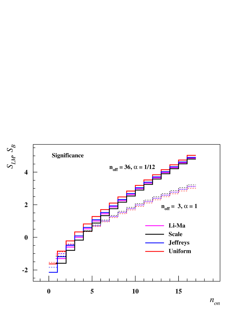
Figure 1: Significances for the source detection are shown as functions of the number of events detected in the on–source zone for two different off–source measurements. In the first case (thick lines), $n_{\rm off}=36$ and $\alpha=\frac{1}{12}$. In the second case (thin lines), $n_{\rm off}=3$ and $\alpha=1$. The Li–Ma significances are shown in magenta. The Bayes significances for scale invariant (black lines), Jeffreys’ (blue lines) and uniform (red lines) prior distributions were derived from the probability of the source presence in the on–source region, see Eq. (9).

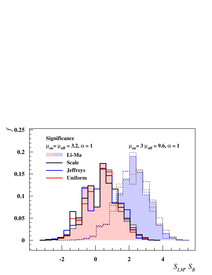
Figure 2: Distributions of significances for the source detection. Histograms for the Li–Ma significances (filled areas) as well as for the Bayes significances using scale invariant (black lines), Jeffreys’ (blue lines) and uniform (red lines) prior distributions are visualized. Two examples for the same exposures of the on– and off–source zones ($\alpha=1$) are presented. In the first example (light red area and thick lines), the on– and off–source counts were generated with the mean parameters $\mu_{\rm on}=\mu_{\rm off}=3.2$. In the second example (light blue area and thin dashed lines), the mean parameters were $\mu_{\rm on}=3\mu_{\rm off}=9.6$.

In the second example, using the Monte Carlo technique, we focused on the distributions of significances for the source detection. We generated $10^{5}$ pairs of on– and off–source counts that follow the Poisson distribution with predefined source and background means, respectively, assuming that they were registered in the regions of the same exposures ($\alpha=1$). We determined the Bayesian probabilities of the source presence in the on–source region (see Eq. (9)) and the corresponding significances as well as the asymptotic Li–Ma significances [2] for each pair of on– and off–source counts. In Fig. 2, we present the significance distributions for no source in the on–source zone, when the on– and off–source means $\mu_{\rm on}=\mu_{\rm off}=3.2$ (light red area and thick lines). Typically, in about $10\%$ of on–off pairs, it happened that no events in the on– or off–source zone were generated. This results in dips in scale invariant (thick black line) and Li–Ma (light red area) histograms located around zero significance since, in such cases, the relevant significances cannot be determined. In Fig. 2, we also show significance distributions that we received in the case when the source is present in the on–source region using $\mu_{\rm on}=3\mu_{\rm off}=9.6$ (light blue and thin dashed lines). In both presented cases, except the problem with zero counts, the significance distributions obtained using the Bayesian inference, with the scale invariant, Jeffreys’ or uniform prior distributions, are similar to each other as well as to the corresponding outputs obtained with the help of the asymptotic Li–Ma formula [2].

3.2 Gamma–ray bursts

The method described in Section 2 was applied to the data sets examined in Refs. [14, 15]. We used information about very high energy (VHE) photons from gamma–ray bursts (GRB) collected by the VERITAS setup [17] and by the Fermi Large Area Telescope [18]. These data sets of VHE photons detected during or shortly after 12 bursts are listed in the first four columns in Table 1. Typically, only a few VHE photons were registered in the directions of GRBs. In most cases, the number of collected events is not too different from the corresponding number of events expected from background.

We assumed the same prior distributions for the on– and off–source means with the common shape parameter, $s=s_{p}=s_{q}$, and zero rate parameters, i.e. $\gamma=\gamma_{p}=\gamma_{q}\to 1$. With these restrictions we calculated the distributions of the difference of the on–source and background means. The probability that a source is absent in the on–source region is then given by Eq. (8). We also determined credible intervals and, if appropriate, upper bounds of the source intensity at a given level of significance as described in Section 2.5.

The conditional distributions of the difference ($\mu_{\rm on}\geq\mu_{\rm b}$) for all data sets are depicted in Fig. 3. These results were obtained with Jeffreys’ prior distributions ($s=\frac{1}{2}$ and $\gamma\to 1$). Specific properties of the GRB sources are summarized in Table 1. In this table, we present the Bayesian probabilities of the absence of a source of VHE photons in the on–source zone ($P^{-}$). Negative values of the corresponding Bayesian significance ($S_{\rm B}$) indicate that the absence of a source in the on–source region is more likely than its presence therein, i.e. $P^{-}>0.5$. For all data sets, we also give credible intervals for the difference of the on–source and background means at a $99\%$ level of confidence. With the distributions of the difference conditioned on the non–negative source intensity we reproduce the upper bounds ($\delta^{+}_{+}$) obtained in Ref. [14] at the same level of confidence (see Section 2.4.3).

Table 1: GRB data collected by VERITAS [17], GRB 080825C was observed by Fermi–Lat [18]. The same sets of data as in Refs. [14, 15] are used. GRB assignments, measured counts and on–off parameters $\alpha$ are listed in the first four columns. The Bayesian probability of the absence of a source in the on–source zone ($P^{-}$), corresponding significance ($S_{\rm B}$) and Li–Ma significance ($S_{\rm LM}$) are given in the following three columns. We show credible intervals for the difference ($\langle\delta_{-},\delta_{+}\rangle$) and its upper bounds obtained by assuming that a source may be present only in the on–source zone ($\delta^{+}_{+}$), both at a $99\%$ level of confidence. Confidence intervals for the difference ($\langle\delta_{-},\delta_{+}\rangle_{\rm L}$) derived in the unbounded profile likelihood method [7] at the same level of confidence are given in the rightmost column. For Bayesian results, Jeffreys’ prior distributions ($s=\frac{1}{2}$ and $\gamma\to 1$) were used.

GRB	$n_{\rm on}$	$n_{\rm off}$	$\alpha$	$P^{-}$	$S_{\rm B}$	$S_{\rm LM}$	$\langle\delta_{-},\delta_{+}\rangle$	$\delta^{+}_{+}$	$\langle\delta_{-},\delta_{+}\rangle_{\rm L}$
070419A	2	14	0.057	0.110	1.23	1.08	-1.11, 7.74	6.88	-0.88, 7.34
070521	3	113	0.057	0.923	-1.43	-1.48	-6.86, 2.91	6.12	-6.77, 3.58
070612B	3	21	0.066	0.106	1.25	1.14	-1.50, 8.61	8.00	-1.23, 8.55
080310	3	23	0.128	0.455	0.11	0.03	-3.60, 6.92	7.16	-3.37, 7.08
080330	0	15	0.123	0.932	-1.49		-3.84, 3.43	4.10	-3.38, 2.40
080604	2	40	0.063	0.591	-0.23	-0.33	-3.03, 5.10	6.12	-2.93, 5.66
080607	4	16	0.112	0.080	1.41	1.32	-1.82,10.12	9.17	-1.42, 9.84
080825C	15	19	0.063	$7\,10^{-10}$	6.22	6.36	5.05, 26.60		5.86, 26.12
081024A	1	7	0.142	0.441	0.15	0.01	-2.13, 5.64	5.30	-1.89, 5.19
090418A	3	16	0.123	0.233	0.73	0.64	-2.50, 8.24	7.64	-2.17, 8.01
090429B	2	7	0.106	0.106	1.25	1.12	-1.04, 6.41	6.92	-0.99, 7.41
090515	4	24	0.126	0.282	0.58	0.50	-3.25, 8.63	8.34	-2.94, 8.66

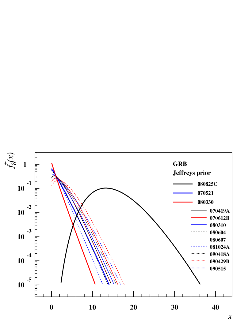
Figure 3: Distributions of the difference conditioned on non–negative values of the on–source rate for 12 data sets connected with GRB observations [17, 18]. These results were obtained with Jeffreys’ prior distributions for the on– and off–source means ($s=\frac{1}{2}$ and $\gamma\to 1$). Full black, blue and red curves are for GRB 080825C, GRB 070521 and GRB 080330, respectively.

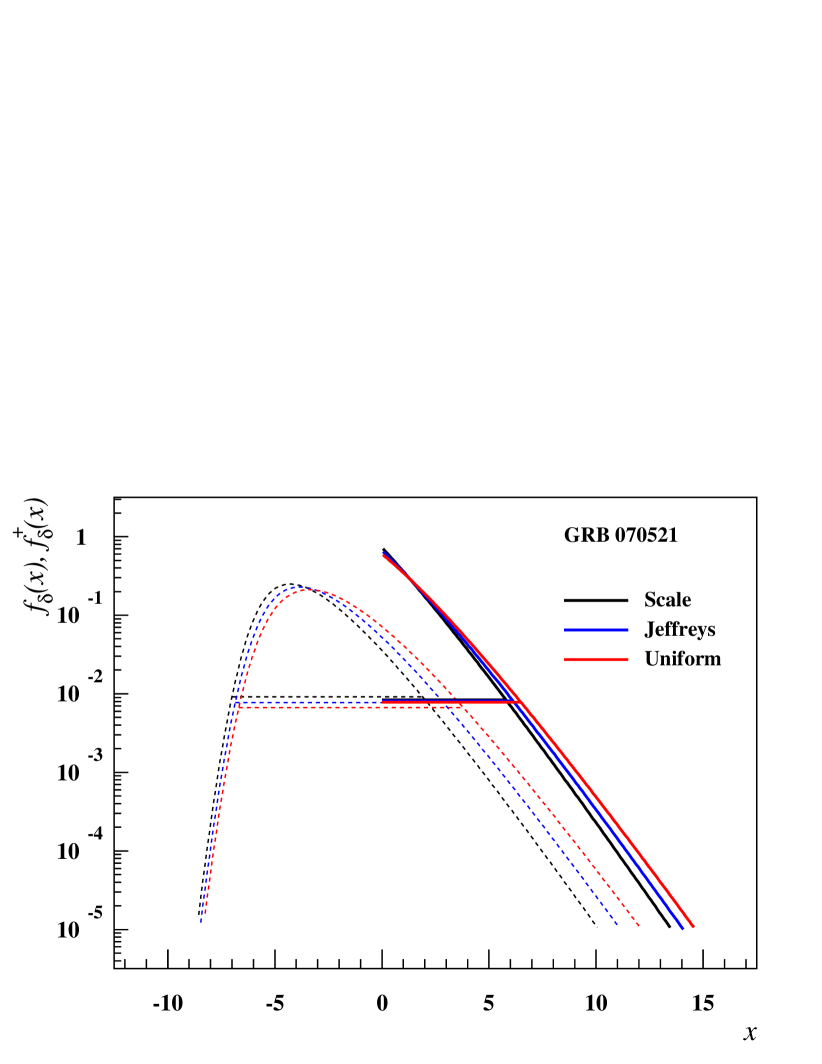
Figure 4: Distributions of the difference using the GRB 070521 data. The distributions shown in black, blue and red were obtained with scale invariant ($s\to 0$), Jeffreys’ ($s=\frac{1}{2}$) and uniform ($s=1$) priors, respectively. The thick full curves are for the distributions determined by assuming that a source may be present only in the on–source zone. The dashed lines indicate solutions without this information. Horizontal lines visualize credible intervals at a $99\%$ level of confidence.

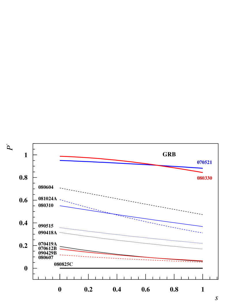
Figure 5: Probabilities of the source absence in the on–source zone are shown as functions of the common shape parameter of prior distributions. The thick full black, blue and red curves are for GRB 080825C, GRB 070521 and GRB 080330, respectively.

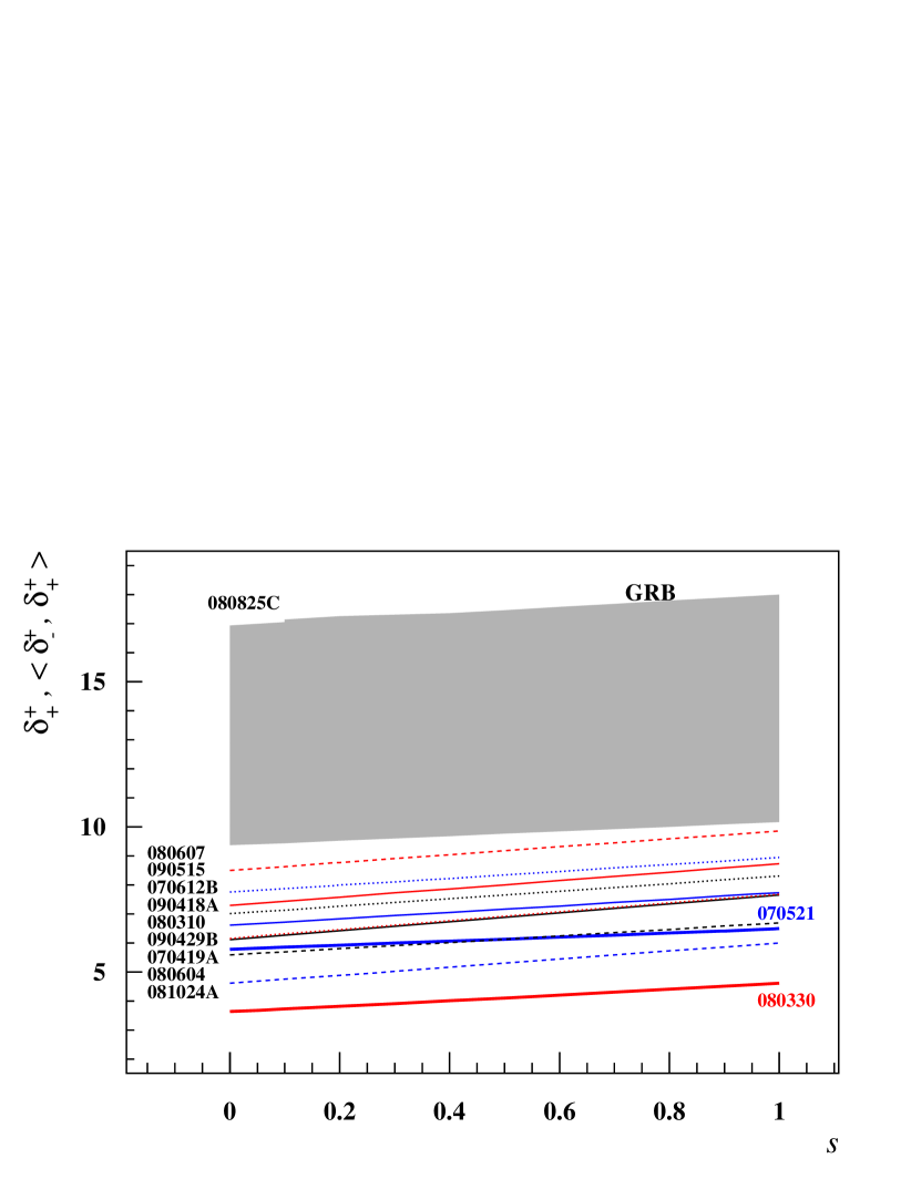
Figure 6: Upper bounds for the difference at a $99\%$ level of confidence are shown as functions of the common shape parameter of prior distributions. They were obtained by assuming that a source may be present only in the on–source zone. The thick full blue and red curves are for GRB 070521 and GRB 080330, respectively. A grey band represents the $1\sigma$ credible interval for the activity associated with GRB 080825C.

In Table 1, we also present other on–off results which were obtained within the classical concept and have, therefore, a different meaning. In particular, we calculated the Li–Ma significance [2]. Also confidence intervals derived using the unbounded likelihood method [7] were determined. It is worth stressing that both these classical statistics are obtained asymptotically relying upon the likelihood ratio and the Wilks’ theorem [1]. The asymptotic confidence intervals or upper bounds are constructed in such way that they cover an unknown true value of the parameter under consideration with a specified probability. The Li–Ma significance corresponds to the probability with which the null background hypothesis is rejected if it is true. We added a sign to the Li–Ma statistic $S_{\rm LM}$ in order that $S_{\rm LM}<0$ if $n_{\rm on}-\alpha n_{\rm off}<0$.

There is a clear evidence that VHE photons from GRB 080825C were detected by the Fermi–Lat instrument [18]. The significance of the presence of a source in the on–source zone, $S_{\rm B}=6.22$, provides the same conclusion as the asymptotic Li–Ma significance, as the original finding [18] and other results [14, 15]. Our $1\sigma$ estimate of the source intensity, $\delta\in\langle 9.75,17.49\rangle$ obtained with Jeffreys’ prior distributions, corresponds to previously presented estimates [14, 15, 18].

Other data sets of VHE photons collected in the directions of GRBs show no signature that would distinguish them from background data. The Bayesian probabilities of the absence of a source in the selected on–source regions are above $8\%$, see Table 1. The absolute values of the corresponding significance are below $1.50$. Three data sets indicate a deficit of events in the on–source region, i.e. $P^{-}>0.5$ and $S_{\rm B}<0$.

Of particular interest are the results derived from the data associated with GRB 080330 since no on–source event was recorded in this observation. We recall that the data is easy to evaluate in the Bayesian approach. No special assumptions or external constraints are needed. The only exception is that the choice of the scale invariant priors ($s\to 0$) is excluded. Using Jeffreys’ prior distributions, our analysis yields the Bayesian probability of the absence of a source in the on–source zone of about $93\%$, see Table 1. Our upper bound for the source intensity is somewhat higher than the estimate which was obtained by extrapolation within the unbounded likelihood method [7].

With the aim to demonstrate the impact of different prior distributions, we choose the data set of GRB 070521. This data yields the lowest positive ratio of the number of on–source events with respect to the background counts expected in the on–source region. In Fig. 4, various distribution functions of the difference for GRB 070521 are shown. Three types of prior distributions were examined. Namely, we present results based on the scale invariant ($s\to 0$, in black), Jeffreys’ ($s=\frac{1}{2}$, blue) and uniform ($s=1$, red) prior distributions. The depicted distributions were obtained without (dashed curves) or with (full curves) assuming that a source may be present only in the on–source zone. The former distributions are used in order to determine the probability of the source presence in the on–source zone. The latter conditional distributions are then used for estimating credible intervals or upper bounds of the source intensity.

In this case, and also for other data sets listed in Table 1, we mostly obtained very similar results for the three types of prior distributions used for the on– and off–source means. This situation is documented in Fig. 5 where the Bayesian probabilities for the source absence in the on–source zone are shown as functions of the common shape parameter of the prior distributions. The no–source probabilities mostly slowly decrease with the increasing value of the prior shape parameter, from the scale invariant option ($s\to 0$) down to the uniform choice ($s=1$). The largest decline is found for the data associated with the observation of GRB 081024A when the lowest total number of events was detected.

Finally, the $99\%$ upper bounds of the source intensity, and the $1\sigma$ credible interval in case of 080825C, are depicted in Fig. 6 as functions of the common shape parameter of the prior distributions. These characteristics were obtained by assuming that a source may be present only in the on–source region. We learned that the limits of the source intensity are weakly dependent on the prior choice of the common shape parameter for $0<s\leq 1$.

4 Conclusions

In this study we dealt the issue of detection of a source the activity of which is immersed in the surrounding background. For this purpose, we adopted the Bayesian concept that provides, on one side, a unified and intuitively appealing approach to the problem of drawing inferences from observations and, on the other side, it offers a powerful and sufficiently general framework for determining optimal behavior in the face of uncertainty. As often reported, the Bayesian inference also allows us to alleviate some of the issues that affect conventional statistical approaches.

We have proposed a consistent description of the on–off measurement. We focused on cases of small numbers of registered events that obey a Poisson distribution. For the on– and off–source means, we used an adequately large class of conjugate prior distributions for the Poisson likelihood function. It consists of Gamma distributions, each of which is parametrized by two parameters, by the rate and shape parameter. The Gamma family includes several interesting and widely used options, i.e. scale invariant, uniform or Jeffreys’ prior distributions.

We examined the distribution of the difference between the on–source and background means. This distribution is maximally noncommittal with regard to their dependence, but it carries all the information available from the on–off experiment. Using it, the probability of the presence of a source in the on–source zone and other source properties are consistently derived within the Bayesian concept and, therefore, have well defined meaning. We stress that our interpretation of the on–off data is different from reasoning behind hypothesis testing, regardless of whether the test is conducted in a classical or Bayesian framework.

The distribution of the difference is well suited for weak sources whose observations may reveal a signal either in the on–source or off–source zone, due to experimental limitations, for example. Except one case, the proposed Bayesian solutions can be used for any number of on–off counts, including the null experiment or the experiment with no background. To our knowledge, such results of the Bayesian inference have not yet been discussed in the literature. By conditioning on the values of the difference we obtained a probability distribution that allows us to describe the on–off problem with a preassigned source in the on–source region the activity of which is to be examined. In this case, the resultant conditional distribution includes several results that have previously been obtained in other Bayesian approaches. Using this distribution, well reasoned limits of the source activity are easily determined.

We also presented several numerical examples that may serve as guides for practical applications. In most cases, when little is known about investigated phenomena, it turned out that the scale invariant, if applicable, or uniform prior distributions are good choices. The corresponding formulae reduce to simple algebraic sums, as described in Sections 2.4.1 and 2.4.2 provided that a source may be present only in the on–source zone. The Bayesian inference using Jeffreys’ prior distributions should be a better compromise. However, this option, as well as the choice of informative priors, requires more complicated calculations based on integral expressions.

Appendix A Bayesian inference with Poisson likelihood

We consider that the number of events registered in a counting experiment, a random variable $n$, obeys the Poisson distribution with a mean $\mu>0$, i.e. $n\sim{\rm Po}(\mu)$. The probability to observe $n$ events ($n=0,1,\dots$) is

$$P_{\rm Po}(n\mid\mu)=\frac{\mu^{n}}{n!}e^{-\mu}.$$ (29)

Our aim is to deduce some information about the Poisson mean $\mu$ from a measurement in which $n$ counts were registered. For this purpose, we adopt the Bayesian reasoning. The probability distribution of the Poisson mean to have the value $\mu>0$ is found by means of Bayes’ theorem

$$f(\mu\mid n)\propto L(\mu\mid n)p(\mu),$$ (30)

where $L(\mu\mid n)=P_{\rm Po}(n\mid\mu)$ is the likelihood function and $p(\mu)$ denotes the prior distribution of the mean $\mu$.

The problem is solved once we specify the form of the prior distribution. To this end, we use Gamma distributions that provide a family of conjugate prior distributions for the Poisson likelihood function

$$p(\mu)=f_{\rm Ga}(\mu\mid s,\lambda)=\frac{\lambda^{s}}{\Gamma(s)}\mu^{s-1}e^{-\lambda\mu},$$ (31)

where $s>0$ is the shape parameter, $\lambda>0$ denotes the rate parameter and $\Gamma(s)$ is the Gamma function. Notice that the mean and variance of a random variable obeying the Gamma distribution are ${\rm E}(\mu)=\lambda^{-1}s$ and ${\rm Var}(\mu)=\lambda^{-2}s$, respectively. Hence, with the increasing value of the shape parameter $s$, the prior distribution is peaked at larger values around a mode $\lambda^{-1}(s-1)$. With the increasing value of the rate parameter $\lambda$, that shifts the position of the mean towards lower values, the prior distribution becomes narrower.

The Gamma family of prior distributions is sufficiently large. The two prior parameters $s$ and $\lambda$ may be chosen to contain our degree of belief about the problem before the experiment is conducted. Notice that traditionally accepted prior assumptions about the studied parameter are included among these possibilities. For example, in a limiting case, if $\lambda\to 0$, the choice $s=1$ represents the uniform prior, $s=\frac{1}{2}$ is for the Jeffreys’ prior (see B) and, if $n>0$, then the scale invariant prior distribution with $s\to 0$ may be selected.

The posterior distribution of the Poisson mean $\mu$ then depends on the prior choice and experimental data. If $n$ events were collected, one easily finds that $\mu\sim{\rm Ga}(p,\gamma)$, where $p=n+s>0$ and $\gamma=\lambda+1>1$, follow from Eq. (30) for the prior distributions chosen from the Gamma family defined in Eq. (31). Hence, the posterior distribution function is

$$f(\mu\mid n)=f_{\rm Ga}(\mu\mid p,\gamma)=\frac{\gamma^{p}}{\Gamma(p)}\mu^{p-1}e^{-\gamma\mu}.$$ (32)

Let us finally note, that for the random variable $\mu^{\prime}=k\mu$, where $k>0$ is a constant, one obtains $\mu^{\prime}\sim{\rm Ga}(p,\frac{\gamma}{k})$.

Appendix B Jeffreys’ prior

By definition, the Jeffreys’ prior is proportional to the square root of the determinant of the Fisher information. In the case of a single–valued Poisson mean $\mu>0$, it is written

$$p(\mu)\propto\sqrt{-{\rm E}\left[\frac{\partial^{2}\ln L(\mu\mid n)}{\partial^{2}\mu}\right]}=\frac{1}{\sqrt{\mu}},$$ (33)

where $L(\mu\mid n)=P_{\rm Po}(n\mid\mu)$ is the likelihood function given in Eq. (29) and ${\rm E}$ denotes the mean value with respect to the Poisson model under study.

Acknowledgment: We would like to thank the two unknown reviewers for their constructive criticism and many useful suggestions that helped us with the presentation of our study. This work was supported by the Czech Science Foundation under project 14-17501S.

References

- [1] S.S.Wilks, Ann.Math.Stat. 9 (1938) 60.
- [2] T.P.Li, Y.Q.Ma, Astrophys.J. 272 (1983) 317.
- [3] R.D.Cousins, J.T.Linnemann, J.Tucker, Nucl.Instrum.Methods A 595 (2008) 480.
- [4] G.Cowan, K.Cranmer, E.Gross, O.Vitells, Eur.Phys.J. C71 (2011), 1554; G.Cowan, K.Cranmer, E.Gross, O.Vitells, Eur.Phys.J. C73 (2013) 2501.
- [5] G.J.Feldman, R.D.Cousin, Phys.Rev. D57 (1998) 3873.
- [6] R.D.Cousins, Nucl.Instrum.Methods A 417 (1998) 391.
- [7] W.A.Rolke, A.M.López, J.Conrad, Nucl.Instrum.Methods A 551 (2005) 493.
- [8] O.Helene, Nucl.Instrum.Methods 212 (1983) 319.
- [9] O.Helene, Nucl.Instrum.Methods 228 (1984) 120.
- [10] H.B.Prosper, Nucl.Instrum.Methods A 241 (1985) 236.
- [11] H.B.Prosper, Phys.Rev. 37 (1988) 1153.
- [12] S.Gillesen and H.L.Harney, Astron.Astrophys. 430 (2005) 355.
- [13] P.Gregory, Bayesian Logical Data Analysis for the Physical Sciences, Cambridge, Cambridge University Press, 2005, (Chapter 14).
- [14] M.L.Knoetig, Astrophys.J. 790 (2014) 106.
- [15] D.Casadei, Astrophys.J. 798 (2015) 5.
- [16] F.W.J.Olver, D.M.Lozier, R.F.Boisvert, C.W.Clark (eds.), NIST Handbook of Mathematical Functions, Cambridge University Press, Cambridge, 2010, (Chapters 8, 13 and 15).
- [17] V.A.Acciari et al., Astrophys.J. 743 (2011) 62.
- [18] A.A.Abdo et al., Astrophys.J. 707 (2009) 580.