Probing New Physics Scales from Higgs and Electroweak Observables at $\bm{e^{+}e^{-}}$ Higgs Factory

Abstract

New physics beyond the standard model (SM) can be model-independently formulated via dimension-6 effective operators, whose coefficients (cutoffs) characterize the scales of new physics. We study the probe of new physics scales from the electroweak precision observables (EWPO) and the Higgs observables (HO) at the future $e^{+}e^{-}$ Higgs factory (such as CEPC). To optimize constraints of new physics from all available observables, we establish a scheme-independent approach. With this formulation, we treat the SM electroweak parameters and the coefficients of dimension-6 operators on equal footing, which can be fitted simultaneously by the same $\chi^{2}$ function. As deviations from the SM are generally small, we can expand the new physics parameters up to linear order and perform an analytical $\chi^{2}$ fit to derive the potential reach of the new physics scales. We find that the HO from both Higgs produnction and decay rates can probe the new physics scales up to 10 TeV  (and to 44 TeV for the case of gluon-involved operator $\mathcal{O}_{g}$), and the new physics scales of Yukawa-type operators can be probed by the precision Higgs coupling measurements up to ($13-25$) TeV. Further including the EWPO can push the limit up to $35$ TeV. From this prospect, we demonstrate that the EWPO measured in the early phase of a Higgs factory can be as important as the Higgs observables. These indirect probes of new physics scales at the Higgs factory can mainly cover the energy range to be directly explored by the next generation hadron colliders of $pp\,(50-\!100$ TeV), such as the SPPC and FCC-hh.
. JHEP (2016), in Press $[$arXiv:1603.03385$]$

1 Introduction

The LHC discovery Higgs12 of a light Higgs boson $h(125\text{GeV})$ Higgs has completed the particle spectrum of the standard model (SM) of particle physics. This culminates in the success of searches that lasted for decades HiggsProfile . Although the new physics has not yet been established so far, there are already strong motivations for going beyond the SM, including the observed neutrino oscillations and cosmic baryon asymmetry, as well as evidences for the dark matter and inflation. Since 2012, the particle physics has come to a turning point at which the precision Higgs measurements have become an important task for seeking clues to the new physics discovery Ellis .

We should stress that the SM is not merely a collection of various observed particles (fermions and bosons). The completion of the SM particle spectrum does not mean the completion of the SM itself until all SM interaction forces could be firmly measured. In fact, the SM consists of three fundamental gauge forces as its key ingredients, the electromagnetic force, the weak force, and the strong force, which are mediated by spin-1 gauge bosons, the photon ($A_{\mu}$), the weak bosons $(W_{\mu}^{\pm},Z_{\mu}^{0})$, and the gluons $(G_{\mu}^{a})$, respectively. Furthermore, the spin-0 Higgs boson $h(125\text{GeV})$ is not merely another particle in the SM, because it joins three types of fundamental forces: (i) the gauge forces mediated by the spin-1 weak gauge bosons $(W,Z)$; (ii) the Yukawa forces with fermions mediated by the spin-0 Higgs boson $h$; (iii) and the cubic and quartic Higgs self-interactions  $h^{3}$ and $h^{4}$ .  Among these, the type-(ii) and type-(iii) are new forces solely mediated by the Higgs boson itself.  They are largely untested so far, and provide the most likely places to encode new physics beyond the SM. Even for the type-(i) force, the LHC Run-2 could only measure the $hWW$ and $hZZ$ couplings down to $(10-20)$% at $2\sigma$ level Peskin . It should be stressed that the discovery of the SM is not complete until all three types of Higgs-involved forces are fully tested by direct measurements.

The existence of such a spin-0 Higgs boson  $h(125\text{GeV})$  is truly profound. This is because $\,h$  is responsible for mass-generations for all SM particles, the spin-1 weak gauge bosons and the spin-$\frac{1}{2}$ quarks and leptons,  via the above type-(i) and type-(ii) forces. Note that the observed unnaturally large hierarchies among the quark and lepton masses correspond to the same hierarchies among the Higgs Yukawa couplings. These Yukawa couplings range from the top quark Yukawa coupling $\,y_{t}\simeq 1\,$ down to a tiny electron Yukawa coupling $\,y_{e}=\mathcal{O}(10^{-6})$,  and have a rather irregular pattern, which are all unexplained within the SM. Hence, the Yukawa sector apparently calls for new physics. The upper bounds on the new physics scales associated with all SM fermion mass-generations vary within the range of $\,3.5-107$ TeV, from the top quark to the electron Dicus:2004rg . This range of scales are mainly beyond the reach of the LHC, but are within the (in)direct reaches of the next generation of high energy circular colliders Nima Dicus:2004rg . The Higgs boson $h$ also generates a physical mass $\,M_{h}\,$ for itself via its type-(iii) self-interaction force after spontaneous symmetry breaking, but this mass is not protected against radiative corrections, causing the naturalness problem HP . Furthermore, this Higgs boson could serve as the inflaton to drive the required exponential expansion of the early universe HINF , and may also be connected to dark matter DM . But, the SM Higgs potential suffers instability at scales well below the Planck mass vacIn and calls for new physics at or beyond the TeV scale TeV .

The above physics considerations strongly motivate the next generation high energy colliders beyond the LHC. Because of the profound implications of the newly discovered light Higgs boson  $h(125\text{GeV})$,  it is natural to first precisely measure its properties at an $e^{+}e^{-}$ Higgs factory and find compelling clues to the new physics. There are three major proposals on the market, the Circular Electron Positron Collider (CEPC) CEPC , the Future Circular Collider (FCC-ee) FCC-ee , and the International Linear Collider (ILC) ILC . All three proposed colliders can run at $\sqrt{s}=250$ GeV  by producing Higgs boson via Higgsstrahlung ($e^{+}e^{-}\!\!\rightarrow Zh$) and $WW$ fusion ($e^{+}e^{-}\!\!\rightarrow\nu\bar{\nu}h$). By measuring decay products of the final state $Z$ boson in the Higgsstrahlung process, the Higgs signal can be extracted with the aid of recoil mass reconstruction technique recoil . This allows model-independent measurement of Higgs decay branching fractions down to percentage level. The CEPC runs at the collision energy of 250 GeV with 5 ab^-1 integrated luminosity can produce about 1 million Higgs bosons. With these, most Higgs decay channels can be precisely measured with sizable events. Hence, such a Higgs factory will be an ideal place to probe the new physics deviations via Higgs production and decays, as well as other precision measurements.

In this work, we will study the probe of new physics scales at the $e^{+}e^{-}$ Higgs factory, with CEPC as a concrete example. For such a Higgs factory, all the new physics effects associated with the light Higgs boson $h(125\text{GeV})$ can be parametrized by model-independent dimension-6 effective operators, which involve the SM Higgs doublet $H$. We will establish a scheme-independent approach to optimize the constraints of new physics from all available observables, including both the electroweak precision observables (EWPO) and the Higgs observables (HO). With this formulation, we treat the SM electroweak parameters and the coefficients of dimension-6 operators on equal footing for a combined analysis, which can be fitted simultaneously by the same $\chi^{2}$ function. Since deviations from the SM are generally small, we can expand the new physics parameters up to linear order and perform an analytical $\,\chi^{2}\,$ fit to derive the potential reach of the new physics scales. We will demonstrate that the $Z$-pole measurements in the early phase of a Higgs factory can be as important as the Higgs observables. Some aspects of the effects of these operators on Higgsstrahlung production were studied before for $e^{+}e^{-}$ colliders at various energies and with different focuses pre , which usually did not cover a complete list of these operators, and also did not consider the interplay with precision observables. A recent paper Craig:2014una studied the probe of these operators at a Higgs factory in the $Z$-scheme by taking the three most precisely measured electrowaek observables (the fine structure constant $\alpha$, the Fermi constant $G_{F}$, and the $Z$ boson mass $M_{Z}$) as fixed inputs. The extended studies considered the existing electroweak precision observables at LEP Falkowski:2014tna , and the measurements at a future Higgs factory Ellis:2015sca . But a comprehensive investigation to combine the constraints of all HO and EWPO would be highly beneficial.

This paper is organized as follows. In Sec. 2, we first establish a scheme-independent approach with linear expansion, which puts both dimension-6 operators and electroweak parameters on equal footing for fitting the data. In Sec. 3, we analyze the CP-conserving dimension-6 effective operators that involve the SM Higgs doublet $H$, and summarize their effects on the field redefinition, particle masses, and interaction vertices, along with Appendix A on kinetic mixing of gauge bosons. With these, in Sec. 4, we study the Higgs and precision observables to deduce the reach of new physics scales that can be probed at the $e^{+}e^{-}$ Higgs factory. Then, in Sec. 5, we present the reach of precision measurement of the SM Higgs couplings at the CEPC, and apply this to study the probe of new physics scales associated with the dimension-6 Yukawa-type operators. Finally, we conclude in Sec. 6. We also present our method of the analytic linear $\chi^{2}$ fit in Appendix B, which is used for the current analyses in Sec. 4 and Sec. 5.

2 Scheme-Independent Approach for Precision Observables

The electroweak sector of SM contains three basic parameters, the $SU(2)_{L}$ gauge coupling $\,g$ ,  the $U(1)_{Y}$ gauge coupling  $g^{\prime}$,  and the Higgs vacuum expectation value (VEV) $v$. They can be determined by the existing precision tests, especially the four most precisely measured observables: the $Z$ boson mass $M_{Z}$,  the $W$ boson mass $M_{W}$,  the Fermi constant $G_{F}$,  and the fine structure constant $\alpha$ .  Fixing the electroweak (EW) parameters $(g,g^{\prime},v)$ needs only three observables as inputs. In common practice, one usually adopts either $Z$-scheme ($M_{Z},G_{F},\alpha$) or $W$-scheme ($M_{Z},M_{W},\alpha$) to fix the values of $(g,g^{\prime},v)$.  Picking up which scheme is thus a matter of choice. In addition, the numerical analysis with this approach could only implement the central values of these electroweak observables without including the associated uncertainties. This means, some information from experimental measurements is discarded and the outcome turns out to be scheme-dependent. In the present study, we try to incorporate all precision observables, so we can realize more sensitive probe of the new physics scales of the dimension-6 operators by using all the information available from experiments. The improvement of this new method is minor for the current precision data, but will become significant for analyzing the future precision measurements at the Higgs factory.

Our new strategy is to employ all the precision observables, including both their central values and uncertainties. The values of  $(g,g^{\prime},v)$  are determined by fitting the data altogether with effective operator coefficients [cf. (5)], rather than being expressed as functions of central values of 3 input parameters chosen for the $Z$-scheme or $W$-scheme. In this way, we can utlize all the most precisely measured precision EW observables ($M_{Z},\,M_{W},\,G_{F},\,\alpha$) altogether with any other relevant observables in our $\chi^{2}$ fit. We no longer need to invoke the concept of scheme or input parameters. Our analysis only involves model (fitting) parameters and experimental data. The basic EW parameters and the coupling coefficients can be treated equally as the fitting parameters. This will just add three more fitting parameters, but all precision observables can be equally used to constrain the dimension-6 operators.

An observable contains the SM contribution, expressed in terms of the EW parameters, plus the corrections from new physics. When fitting experimental measurements, the SM contribution and new physics contribution vary simultaneously. So long as the precision measurements are included, the EW parameters are constrained with small uncertainties. On the other hand, the new physics contribution is expected to be small. Thus, it is well justified that both the EW parameters and the effective operator coefficients have only small shifts from their reference values. We can expand observables as linear combinations of the shifts. In consequence, we can perform analytic $\chi^{2}$ fit as elaborated in B.

To implement the two features above, we treat all model-parameters (EW parameter and effective operator coefficients) on equal footing and make analytic $\chi^{2}$ fit for small variations. We lay out the procedure as follows. First, we split each EW parameter  $f$  as a sum of the reference value (acting as starting point for the $\chi^{2}$ fit) and the shift from it,

$$f^{(\text{sm})}\,\equiv\,f^{(r)}+\delta f\,\simeq\,f^{(r)}\!\left(\!1+\frac{\delta f}{f}\right),$$ (1)

where $\,f^{(\text{sm})}\,$ is the SM prediction, $\,f^{(r)}\,$ the reference value, and $\delta f$ the shift between them. Note that before fitting the data each of these quantities exists only symbolically and should be treated as a variable without specific value. Then, any observable $\,X\,$ can be expanded in a similar way,

$$X\,\equiv\,X\llbracket f^{(\text{sm})}\rrbracket+\overline{\delta X}\,=\,X\llbracket f^{(r)}\rrbracket+X^{\prime}\llbracket f\rrbracket\delta f\!+\overline{\delta X}\,\equiv\,X^{(r)}\!+\widetilde{\delta X},$$ (2)

where $\,X\llbracket f\rrbracket$  is a functional form of the observable in terms of the EW parameters, while the new physics contribution (which can arise from the relevant dimension-6 operators EFT1 ; EFT2 for instance, cf. Eq. (5) and Table 1) and the SM loop corrections are included in $\,\overline{\delta X}$ .  Corresponding to the reference value $f^{(r)}$ of the EW parameters, the observable also has a reference value $\,X^{(r)}\!\equiv X\llbracket f^{(r)}\rrbracket$ .  Its shift from reference value is then combined into

$$\widetilde{\delta X}\,\equiv\,X^{\prime}\llbracket f\rrbracket\delta f+\overline{\delta X}\,,$$ (3)

where $\,X^{\prime}\llbracket f\rrbracket$  is a functional derivative with respect to $\,f\,$.

For the present study, we use $\,f=(M_{Z},\,G_{F},\,\alpha)$  as EW fitting parameters which are equivalent to using $(g,\,g^{\prime},\,v)$, but have the benefit of being direct physical observables. Each of them contains a shift from its reference value,

$$M^{(\text{sm})}_{Z}\!=M^{(r)}_{Z}\!\left(\!1\!+\!\frac{\delta M_{Z}}{M_{Z}}\right)\!,~{}~{}~{}G^{(\text{sm})}_{F}\!=G^{(r)}_{F}\!\left(\!1\!+\!\frac{\delta G_{F}}{G_{F}}\right)\!,~{}~{}~{}\alpha^{(\text{sm})}\!=\alpha^{(r)}\!\left(\!1\!+\!\frac{\delta\alpha}{\alpha}\right)\!.$$ (4)

The quantities  $(\delta M_{Z},\,\delta G_{F},\,\delta\alpha)$  are the differences between the SM prediction and reference value. Note that the SM prediction can be at either tree-level or loop-level, depending on whether the loop-level correction needs to be taken into consideration. In either case, the dependence on the electroweak parameter shifts remains the same, since the SM loop-contribution is already at the linear order and hence can be treated as a constant term in our linear $\chi^{2}$ fit,  $\delta X_{\mathrm{1-loop}}\llbracket f\rrbracket\simeq\delta X_{\mathrm{1-loop}}\llbracket f^{(r)}\rrbracket$ ,  as long as the reference values are close to the experimental central values so that the effect of the shift $\,\delta f\,$ belongs to higher orders and is negligible at the linear-order perturbation. We will give an explicit example for the case of $W$ boson mass in Sec. 4.1, which justifies that Eq.(4) applies to either tree-level or loop-level analysis.

In principle, the reference point  $f^{(f)}$  can take any value. This arbitrariness is then compensated by the corresponding shift parameter $\,\delta f$ .  Nevertheless, for our linear expansion and thus the analytic $\chi^{2}$ fit to work, the reference point should be close to the best-fit value which is around the experimental central value. When the reference value is fixed to the experimental central value and if no parameter is allowed to be freely adjusted, the shift quantity $\,\widetilde{\delta X}$  would vanish. For our choice of $\,(M_{Z},\,G_{F},\,\alpha)$  as fitting parameter, the assumption of vanishing  $(\widetilde{\delta M_{Z}},\,\widetilde{\delta G_{F}},\,\widetilde{\delta\alpha})$  will reduce our scheme-independent approach to the commonly used $Z$-scheme. For the practical analysis here, we will assign the reference values of $\,(M_{Z},\,G_{F},\,\alpha)$  to be their current experimental central values for convenience and allow their shifts $\,(\delta M_{Z},\,\delta G_{F},\,\delta\alpha)$  to vary for scheme-independent fit (when needed).

3 New Physics from Dimension-6 Effective Operators

In this section, we first present the effective Lagrangian with relevant dimension-6 operators for the current precision Higgs study (Sec. 3.1). Then, we systematically derive their effects via kinetic terms and mass terms (Sec. 3.2), and via interaction vertices (Sec. 3.3).

Table 1: List of dimension-6 effective operators for the present study.

Higgs	EW Gauge Bosons	Fermions
$\mathcal{O}_{H}\!=\frac{1}{2}(\partial_{\mu}|H|^{2})^{2}$	$\mathcal{O}_{WW}\!=g^{2}|H|^{2}W^{a}_{\mu\nu}W^{a\mu\nu}$	$\mathcal{O}^{(3)}_{L}\!=(iH^{\dagger}\sigma^{a}\!\!\stackrel{{\scriptstyle\leftrightarrow}}{{D}}_{\mu}\!\!H)(\overline{\Psi}_{L}\gamma^{\mu}\sigma^{a}\Psi_{L})$
$\mathcal{O}_{T}\!=\frac{1}{2}(H^{\dagger}\!\stackrel{{\scriptstyle\leftrightarrow}}{{D}}_{\mu}\!H)^{2}$	$\mathcal{O}_{BB}\!=g^{2}|H|^{2}B_{\mu\nu}B^{\mu\nu}$	$\mathcal{O}^{(3)}_{LL}\!=(\overline{\Psi}_{L}\gamma_{\mu}\sigma^{a}\Psi_{L})(\overline{\Psi}_{L}\gamma^{\mu}\sigma^{a}\Psi_{L})$
	$\mathcal{O}_{WB}\!=gg^{\prime}H^{\dagger}\sigma^{a}HW^{a}_{\mu\nu}B^{\mu\nu}$	$\mathcal{O}_{L}\!=(iH^{\dagger}\!\stackrel{{\scriptstyle\leftrightarrow}}{{D}}_{\mu}\!H)(\overline{\Psi}_{L}\gamma^{\mu}\Psi_{L})$
Gluon	$\mathcal{O}_{HW}\!=ig(D^{\mu}H)^{\dagger}\sigma^{a}(D^{\nu}H)W^{a}_{\mu\nu}$	$\mathcal{O}_{R}\!=(iH^{\dagger}\!\!\stackrel{{\scriptstyle\leftrightarrow}}{{D}}_{\mu}\!\!H)(\overline{\psi}_{R}\gamma^{\mu}\psi_{R})$
$\mathcal{O}_{g}\!=g_{s}^{2}|H|^{2}G^{a}_{\mu\nu}G^{a\mu\nu}$	$\mathcal{O}_{HB}\!=ig^{\prime}(D^{\mu}H)^{\dagger}(D^{\nu}H)B_{\mu\nu}$	$\mathcal{O}_{y}^{u}=|H|^{2}\,\overline{\Psi}_{L}^{q}\tilde{H}u_{R}$
	$\mathcal{O}_{W}=\mbox{$\frac{{ig}}{2}$}(H^{\dagger}\!\sigma^{a}\!\!\stackrel{{\scriptstyle\leftrightarrow}}{{D}}_{\mu}\!\!H)D_{\nu}W^{a\mu\nu}$	$\mathcal{O}_{y}^{d}=|H|^{2}\,\overline{\Psi}_{L}^{q}{H}d_{R}$
	$\mathcal{O}_{B}=\mbox{$\frac{{ig^{\prime}}}{2}$}(H^{\dagger}\!\stackrel{{\scriptstyle\leftrightarrow}}{{D}}_{\mu}\!\!H)D_{\nu}B^{\mu\nu}$	$\mathcal{O}_{y}^{\ell}=|H|^{2}\,\overline{\Psi}_{L}^{\ell}{H}\ell_{R}$

3.1 Effective Lagrangian with Dimension-6 Operators

The new physics effects beyond the SM can be generally parametrized by the dimension-6 effective operators in a model-independent way EFT1 ; EFT2 ,

$$\mathcal{L}~{}=~{}\mathcal{L}_{\text{SM}}+\sum_{j}\frac{c_{j}}{\,\Lambda^{2}\,}\mathcal{O}_{j}\,.$$ (5)

If these new physics effects are associated with Higgs boson, we expect a set of gauge-invariant and CP-conserving dimension-6 operators will appear in the low energy effective theory, as summarized in Table 1. We expect the associated cutoff scale $\,\Lambda/{|c_{j}|^{\frac{1}{2}}}\,$ to be around TeV scale or not far above it. Since the physical processes at an $e^{+}e^{-}$ Higgs factory with $\,\sqrt{s}=240-250$ GeV  have energy scales well below the TeV scale, we see that the effective Lagrangian (5) provides a perfectly valid low energy formulation of the new physics effects.

This effective Lagrangian contains ten bosonic and seven fermionic dimension-6 operators, where each operator is associated with its own coefficient $\,c_{j}/\Lambda^{2}$.  We note that integration by part gives the identities eom ,

$$\mathcal{O}_{B} = \,\mathcal{O}_{HB}+\frac{1}{4}\left(\mathcal{O}_{BB}\!+\mathcal{O}_{WB}\right),$$ (6a)

$$\mathcal{O}_{W} = \mathcal{O}_{HW}+\frac{1}{4}\left(\mathcal{O}_{WW}\!+\mathcal{O}_{WB}\right).$$ (6b)

It means that among the seven operators ($\mathcal{O}_{B}$, $\mathcal{O}_{W}$, $\mathcal{O}_{BB}$, $\mathcal{O}_{WB}$, $\mathcal{O}_{WW}$, $\mathcal{O}_{HB}$, $\mathcal{O}_{HW}$), two of them are redundant. We could use these to eliminate ($\mathcal{O}_{B},\,\mathcal{O}_{W}$), which is called the HISZ basis in the literature basis . We further note that the operators ($\mathcal{O}_{B},\,\mathcal{O}_{W}$) can be replaced by the equation of motion (EOM) eom ,

$$\mathcal{O}_{B} = \,{{g^{\prime}}^{2}}\!\left[-\mbox{$\frac{{1}}{2}$}\mathcal{O}_{T}+\mbox{$\frac{{1}}{2}$}(Y_{L}\mathcal{O}_{L}+Y_{R}\mathcal{O}_{R})\right]\!,$$ (7a)

$$\mathcal{O}_{W} = \,g^{2}\!\left[-\mbox{$\frac{{3}}{2}$}\mathcal{O}_{H}+2\mathcal{O}_{6}+\mbox{$\frac{{1}}{2}$}\left(\mathcal{O}_{y}^{u}+\mathcal{O}_{u}^{d}+\mathcal{O}_{y}^{\ell}+\textrm{h.c.}\right)+\mbox{$\frac{{1}}{4}$}\mathcal{O}_{L}^{(3)}\right]\!,$$ (7b)

where $\,Y_{L}\,$ and $\,Y_{R}\,$ stand for the hypercharges of fermion fields $\Psi_{L}$ and $\Psi_{R}$, respectively. Eqs. (7a)-(7b) also make ($\mathcal{O}_{B},\,\mathcal{O}_{W}$) redundant. Thus, one may use the identities (6a)-(6b) to eliminate the two other operators ($\mathcal{O}_{WW},\,\mathcal{O}_{WB}$) instead. This means that the four operators ($\mathcal{O}_{B},\,\mathcal{O}_{W}$) and ($\mathcal{O}_{WW},\,\mathcal{O}_{WB}$) are redundant, and can be eliminated in principle. For the current first-step study, with the limited experimental observables and a large number of dimension-6 effective operators, we will not carry out a global $\chi^{2}$ fit of all operators together. Instead, we perform the $\chi^{2}$ fit by including only one operator at each time, which is common in the literature. So we need not to exclude the redundant operators. In this way, we can first examine how each operator contributes and how it can be constrained, for completeness. Nevertheless, in the current study, we will always impose the basic identities (6a)-(6b) to eliminate ($\mathcal{O}_{B},\,\mathcal{O}_{W}$), as is the commonly used HISZ basis basis . [But we stress that when considering a future global $\chi^{2}$ fit including many operators simultaneously, it is necessary to remove all the redundant operators by using both the identities (6) and the EOM (7).]

Note that in Table 1, $\mathcal{O}^{(3)}_{LL}$ does not involve the SM Higgs doublet, but we take it into account since it affects the Fermi constant (which is the coefficient of dimension-6 four-fermion operator itself), and consequently the other observables through parameter shift. Since each of the Yukawa-type effective operators $(\mathcal{O}_{y}^{u},\,\mathcal{O}_{y}^{d},\,\mathcal{O}_{y}^{\ell})$ modifies the SM Yuakawa coupling only by a rescaling factor, we study their tests separately in Section 5.

If the underlying UV theory for these effective operators is known, their coefficients could be expressed in terms of the model-parameters in principle. For the present study, we follow the model-independent effective theory formulation, where the coefficients of dimension-6 operators are independent of each other. We will use experimental measurements to estimate the potential reach of indirectly probing the effective new physics scale $\,\Lambda_{j}\equiv\Lambda/{|c_{j}|^{\frac{1}{2}}}\,$ associated with each operator at the Higgs factory (cf. Sec. 4).  We will keep in mind that the coefficient $\,c_{j}\,$ of each effective operator $\,\mathcal{O}_{j}\,$ usually depends on powers of the couplings from the underlying UV theory, which could be larger or smaller than $\,\mathcal{O}(1)$.  The coefficient $\,c_{j}\,$ could also depend on loop-factors when $\,\mathcal{O}_{j}\,$ is induced from loop-level contributions (such as the case of $\,\mathcal{O}_{g}\,$). Hence, it is a model-dependent issue to further convert our general bound on $\,\Lambda_{j}\,$ to the corresponding bound on $\,\Lambda\,$.  In the rest of this section, we first analyze the contributions of these dimension-6 operators to the relevant Feynman vertices and physical observables.

3.2 New Physics via Kinetic Terms and Mass Terms

Before drawing Feynman diagrams and computing the relevant Higgs production cross sections and decay width, it is necessary to check whether all the involved propagators take their canonical form. If not, we need to make proper field redefinitions as summarized in Appendix A. Such redefinitions will modify the relevant mass terms and interaction vertices. With the dimension-6 operators in Table 1, the kinetic terms of fermions remain the same, while those of bosonic fields, the Higgs field $h$ and the gauge bosons ($W^{\pm},\,Z^{0},\,A^{0}$), are affected.

3.2.1 Higgs Field $h$

The operator $\mathcal{O}_{H}$ in Table 1 could contribute a nonzero correction to the kinetic term of the Higgs field. Redefining the Higgs field,

$$h~{}\rightarrow~{}\left(1-\frac{1}{2}\frac{v^{2}}{\Lambda^{2}}c_{H}\right)h\equiv Z_{h}h,$$ (8)

will absorb the deviation from the canonical form. It applies to every $h$ that appears in the Lagrangian and leads to a rescaling factor for any interaction vertex involving Higgs field(s). Each Higgs field $h$ receives a rescaling factor $Z_{h}$, and Higgs mass term receives a rescaling factor $Z^{2}_{h}$.

3.2.2 Charged Gauge Boson

The $W^{\pm}$ gauge bosons receive a correction to its kinetic term from the operator $\mathcal{O}_{WW}$ in Table 1. This leads to the field redefinition of the $W^{\pm}$ bosons,

$$W^{\pm}~{}\rightarrow~{}\left(1+\frac{v^{2}}{\Lambda^{2}}g^{2}c_{WW}\right)W^{\pm}\,\equiv\,Z_{W}W^{\pm}.$$ (9)

Although the $W$ mass receives no direct correction, the field redefinition and parameter shift can contribute indirectly,

$$\frac{\widetilde{\delta M_{W}}}{M_{W}}\,=\,\frac{1}{c^{2}_{w}-s^{2}_{w}}\left[c^{2}_{w}\frac{\delta M_{Z}}{M_{Z}}+\frac{1}{2}s^{2}_{w}\left(\frac{\delta G_{F}}{G_{F}}-\frac{\delta\alpha}{\alpha}\right)\right]+\frac{v^{2}}{\Lambda^{2}}g^{2}c_{WW}\,,$$ (10)

according to (63). The weak mixing angle is denoted as $(c_{w},s_{w})\equiv(\cos\theta_{w},\sin\theta_{w})$ evaluated at the reference point. Note that the correction from field redefinition to the mass term has the same sign as in (9).

3.2.3 Neutral Gauge Bosons

The case of neutral gauge bosons is a little bit more complicated since both kinetic term and mass term are $2\times 2$ matrices. From the dimension-6 operators $(\mathcal{O}_{WW},\mathcal{O}_{BB},\mathcal{O}_{WB})$ in Table 1, we derive corrections to the kinetic term, $\mathbb{I}\partial^{2}\rightarrow\mathbb{K}\partial^{2}\equiv(\mathbb{I}+\delta K)$, with the explicit form of $\delta K$ given in (73). The neutral $Z$ and $A$ gauge bosons need to be not only redefined but also diagonalized as we elaborate in Appendix A.2,

$$Z^{\mu} \rightarrow \left[1+\frac{v^{2}}{\Lambda^{2}}\left(c^{2}_{w}g^{2}c_{WW}+c_{w}s_{w}gg^{\prime}c_{WB}+s^{2}_{w}g^{\prime 2}c_{BB}\right)\right]\!Z^{\mu},$$ (11a)

$$A^{\mu} \rightarrow \left[1+\frac{v^{2}}{\Lambda^{2}}\left(s^{2}_{w}g^{2}c_{WW}-c_{w}s_{w}gg^{\prime}c_{WB}+c^{2}_{w}g^{\prime 2}c_{BB}\right)\right]\!A^{\mu}$$ (11b)

$$+2\frac{v^{2}}{\Lambda^{2}}\left[c_{w}s_{w}g^{2}c_{WW}-\frac{1}{2}(c^{2}_{w}-s^{2}_{w})gg^{\prime}c_{WB}-c_{w}s_{w}g^{\prime 2}c_{BB}\right]\!Z^{\mu}.$$

For convenience, we denote the field redefinition of $A$ and $Z$ as $A\rightarrow Z_{A}A+\delta Z_{X}Z\equiv(1+\delta Z_{A})A+\delta Z_{X}Z$ and  $Z\rightarrow Z_{Z}Z\equiv(1+\delta Z_{Z})Z$,  respectively, where the explicit form of  $(\delta Z_{A},\,\delta Z_{Z},\,\delta Z_{X})$  can be read off from (11). Note that kinetic mixing can introduce not only field redefinition $(\delta Z_{A},\delta Z_{Z})$ to both $A$ and $Z$, but also equal correction $\delta Z_{X}$ to the left- and right-handed currents of the $Z$ boson from the electromagnetic current as shown in the last line.

Any vertex involving $n$ fields of $Z$ should be divided by a factor of $Z^{n}_{Z}$ due to this field redefinition. The mass term can be treated as a vertex with two gauge fields. Hence, it is rescaled by $Z^{2}_{Z}$. The mass of the neutral gauge boson $Z$ is also affected by $\mathcal{O}_{T}$ in Table 1,

$$\frac{\widetilde{\delta M_{Z}}}{M_{Z}}=\frac{\delta M_{Z}}{M_{Z}}-\frac{1}{2}\frac{v^{2}}{\Lambda^{2}}c_{T}+\delta Z_{Z}\,.$$ (12)

where the extra contribution comes from the field redefinition (11a) of the $Z$ gauge boson as indicated by the general analysis in Appendix A.2.

3.2.4 Gluons

Once the Higgs field $H$ develops nonzero VEV, the operator $\mathcal{O}_{g}$ in Table 1 can induce a correction to the kinetic term of gluons. The effect is a field redefinition,

$$G^{a}_{\mu}\rightarrow\left(1+\frac{v^{2}}{\Lambda^{2}}g^{2}_{s}c_{g}\right)G^{a}_{\mu}\equiv Z_{G}G^{a}_{\mu}\,,$$ (13)

which only affect the relevant interaction vertices.

3.3 New Physics via Interaction Vertices

The new physics parameters of the dimension-6 operators can affect the interaction vertices in three ways. First, they can give direct contributions to the existing vertex, sometimes with a different tensor structure such as the case of $ZZh$ coupling. Second, the field redefinition can introduce an overall rescaling factor of the relevant vertex that contains the corresponding field. Finally, the shifts of electroweak parameters from their reference values can affect the existing vertex through zeroth order correlations. In addition, the dimension-6 operators may introduce some new vertices, such as the trilinear vertex $AZh$, and other quartic interactions $\,Zh\psi\bar{\psi}\,$ and $\,Wh\ell\nu$.

3.3.1 Gauge Boson Coupling with Fermions

The coupling between the charged gauge boson $W^{\pm}$ and leptons can be modified by the operator $\mathcal{O}^{(3)}_{L}$ in Table 1 and the $W$ field redefinition (9),

$$\frac{g}{\sqrt{2}}\left(\frac{v^{2}}{\Lambda^{2}}c^{(3)}_{L}+\frac{v^{2}}{\Lambda^{2}}g^{2}c_{WW}\right)\left(W^{+}_{\mu}\bar{\nu}_{L}\gamma^{\mu}\ell_{L}+W^{-}_{\mu}\bar{\ell}_{L}\gamma^{\mu}\nu_{L}\right).$$ (14)

Note that the direct correction to this vertex has the same form as the SM counterpart. Hence, its contribution can be combined into the overall coupling constant. In addition, $\,g_{W\ell\nu}\,$ can split into the reference value plus parameter shift in $\,g\,$,

$$\frac{\widetilde{\delta g_{W\ell\nu}}}{g_{W\ell\nu}}~{}=~{}\frac{1}{\,\cos 2\theta_{w}\,}\left(c^{2}_{w}\frac{\delta M_{Z}}{M_{Z}}+\frac{1}{2}c^{2}_{w}\frac{\delta G_{F}}{G_{F}}-\frac{1}{2}s^{2}_{w}\frac{\delta\alpha}{\alpha}\right)+\frac{v^{2}}{\Lambda^{2}}c^{(3)}_{L}+\frac{v^{2}}{\Lambda^{2}}g^{2}c_{WW}.$$ (15)

For the $Z\bar{\ell}\ell$ vertex, new physics contributions arise from both direct correction and kinetic mixing. The first part comes from operators $(\mathcal{O}^{(3)}_{L},\mathcal{O}_{L},\mathcal{O}_{R})$ in Table 1,

$$\frac{g}{2c_{w}}\frac{v^{2}}{\Lambda^{2}}\left[\left(c^{(3)}_{L}\!-c_{L}\right)\bar{\nu}_{L}\gamma^{\mu}\nu_{L}-\left(c^{(3)}_{L}\!+c_{L}\right)\bar{\ell}_{L}\gamma^{\mu}\ell_{L}-c^{\nu}_{R}\bar{\nu}_{R}\gamma^{\mu}\nu_{R}-c^{\ell}_{R}\bar{\ell}_{R}\gamma^{\mu}\ell_{R}\right]Z_{\mu}.$$ (16)

We can see that the four terms are independent of each other with four different dimension-6 operator coefficients. In addition, the redefinitions (11) of $(Z,A)$ introduce extra corrections to the left- and right-handed currents,

$$\delta g^{*}_{L} = Q\,g_{z}c_{w}s_{w}\delta Z_{X}+g_{z}(T_{3}-s^{2}_{w}Q)\delta Z_{Z},$$ (17a)

$$\delta g^{*}_{R} = Q\,g_{z}c_{w}s_{w}\delta Z_{X}-g_{z}s^{2}_{w}Q\delta Z_{Z}.$$ (17b)

The first term is universal for left- and right-handed couplings, since it comes from the $Z$-$A$ mixing and most importantly is proportional to the electromagnetic current. On the other hand, the second term comes from the field redefinition of the $Z$ gauge boson, rendering it proportional to the SM prediction of $g_{L}$ and $g_{R}$, respectively. Finally, from the zeroth-order coupling, extra correction can appear through parameter shift. Here we show the correction to the coupling with charged leptons,

$$\widetilde{\delta g_{L}} \equiv -\left[\frac{1}{2\cos 2\theta_{w}}\left(\frac{\delta M_{Z}}{M_{Z}}+\frac{1}{2}\frac{\delta G_{F}}{G_{F}}\right)-\frac{c^{2}_{w}s^{2}_{w}}{\cos 2\theta_{w}}\frac{\delta\alpha}{\alpha}\right]\!g_{z}-\frac{g_{z}v^{2}}{2\Lambda^{2}}\left(c^{(3)}_{L}+c_{L}\right)+\delta g^{*}_{L},\qquad\quad$$ (18a)

$$\widetilde{\delta g_{R}} \equiv -\left[\frac{s^{2}_{w}}{\cos 2\theta_{w}}\left(\frac{\delta M_{Z}}{M_{Z}}+\frac{1}{2}\frac{\delta G_{F}}{G_{F}}\right)-\frac{c^{2}_{w}s^{2}_{w}}{\cos 2\theta_{w}}\frac{\delta\alpha}{\alpha}\right]\!g_{z}-\frac{g_{z}v^{2}}{2\Lambda^{2}}c_{R}+\delta g^{*}_{R},$$ (18b)

where the second term accounts for the direct contribution summarized in (16). For convenience, we use $\,g_{z}\equiv g/\cos\theta_{w}\,$ to denote the weak gauge coupling associated with $Z$ boson.

3.3.2 Gauge Boson Couplings with Higgs

Corrections to the $ZZh$ vertex arise from $(\mathcal{O}_{T},\mathcal{O}_{WW},\mathcal{O}_{BB},\mathcal{O}_{WB},\mathcal{O}_{HW},\mathcal{O}_{HB})$ in Table 1,

$$-\frac{g^{2}v}{2c^{2}_{w}}\frac{v^{2}}{\Lambda^{2}}c_{T}hZ_{\mu}Z^{\mu}+\delta Z_{Z}h\mathcal{Z}_{\mu\nu}\mathcal{Z}^{\mu\nu}+\frac{g}{2}\frac{v\partial_{\mu}h}{\Lambda^{2}}\left[gc_{HW}+\frac{s_{w}}{c_{w}}g^{\prime}c_{HB}\right]Z_{\nu}\mathcal{Z}^{\mu\nu},~{}~{}~{}$$ (19)

where $\mathcal{Z}_{\mu\nu}\equiv\partial_{\mu}Z_{\nu}-\partial_{\nu}Z_{\mu}$.  Note that the Higgs field redefinition (8) also contributes an overall term, $-\delta Z_{h}g_{z}M_{Z}\frac{1}{2}hZ_{\mu}Z^{\mu}$,  which should be combined with the first term that has the same tensor structure as the SM contribution. To keep the expression neat, let us define $\,f^{\mu\nu}\llbracket p,q\rrbracket\equiv p^{\nu}q^{\mu}-(p\cdot q)g^{\mu\nu}$.  Then, the Feynman rule reads,

$$ig_{ZZh}\left\{\left(1+c^{Z}_{0}\right)g^{\mu\nu}+c^{Z}_{1}f^{\mu\nu}\llbracket k_{1},k_{2}\rrbracket+c^{Z}_{2}f^{\mu\nu}\llbracket k_{1},k_{1}\rrbracket+c^{Z}_{3}f^{\mu\nu}\llbracket k_{2},k_{2}\rrbracket\right\},\quad$$ (20)

with $\,g_{ZZh}\equiv gM_{Z}/c_{w}$.  The decomposition (20) is useful when discussing Higgs decay and will be applied to the $W^{+}W^{-}h$ and $AZh$ vertices discussed later in this section. The coefficients $c^{Z}_{i}$ are defined as

$$c^{Z}_{1} = \frac{2}{\Lambda^{2}}\left[4\left(s^{4}_{w}c_{BB}+c^{2}_{w}s^{2}_{w}c_{WB}+c_{w}^{4}c_{WW}\right)-\left(s^{2}_{w}c_{HB}+c^{2}_{HW}\right)\right],$$ (21a)

$$c^{Z}_{2} = c^{Z}_{3}=-\frac{1}{\Lambda^{2}}\left(s^{2}_{w}c_{HB}+c^{2}_{w}c_{HW}\right).$$ (21b)

Note that the overall rescaling factor of the SM contribution has been combined with the $Z$ boson field redefinition (11a) and the parameter shift,

$$c^{Z}_{0}\,=\,\frac{\widetilde{\delta g_{ZZh}}}{g_{ZZh}}\,=\,\frac{1}{2}\frac{\delta G_{F}}{G_{F}}+2\frac{\delta M_{Z}}{M_{Z}}-2\frac{v^{2}}{\Lambda^{2}}\left(c_{T}+\frac{1}{4}c_{H}\right)+2\delta Z_{Z}\,.$$ (22)

The $W^{+}W^{-}h$ vertex is much simpler without complication from kinetic mixing. It receives corrections from $(\mathcal{O}_{WW},\,\mathcal{O}_{HW})$ in Table 1,

$$2g^{2}\frac{vh}{\Lambda^{2}}c_{WW}\mathcal{W}^{+}_{\mu\nu}\mathcal{W}^{-\mu\nu}-\frac{g^{2}}{2}\frac{v\partial_{\mu}h}{\Lambda^{2}}c_{HW}(W^{+}_{\nu}\mathcal{W}^{-\mu\nu}+W^{-}_{\nu}\mathcal{W}^{+\mu\nu}),$$ (23)

where $\mathcal{W}^{\pm\mu\nu}\equiv\partial^{\mu}W^{\pm\nu}-\partial^{\nu}W^{\pm\mu}$. It can be grouped into the same form as (20), with $p_{\pm}$ denoting the momenta of $W_{\pm}$,

$$igM_{W}\left\{\left(1+c^{W}_{0}\right)g^{\mu\nu}+c^{W}_{1}f^{\mu\nu}\llbracket p_{+},p_{-}\rrbracket+c^{W}_{2}f^{\mu\nu}\llbracket p_{+},p_{+}\rrbracket+c^{W}_{3}f^{\mu\nu}\llbracket p_{-},p_{-}\rrbracket\right\},$$ (24)

where the coefficients $c^{W}_{i}$ are defined as

$$c^{W}_{1}=\frac{2}{\Lambda^{2}}\left(4c_{WW}\!+c_{HW}\right),\quad~{}~{}~{}c^{W}_{2}=c^{W}_{3}=\frac{1}{\Lambda^{2}}c_{HW}.$$ (25)

The field redefinitions of $W$ and Higgs field redefinitions, (9) and (8), contribute as an overall rescaling and hence can be combined with the parameter shift,

$$c^{W}_{0}\,=\,\frac{\widetilde{\delta g_{WWh}}}{g_{WWh}}\,=\,\frac{1}{2}\left(2c^{2}_{w}\frac{\delta M_{Z}}{M_{Z}}+\frac{1}{2}\frac{\delta G_{F}}{G_{F}}-s^{2}_{w}\frac{\delta\alpha}{\alpha}\right)-\frac{1}{2}\frac{v^{2}}{\Lambda^{2}}c_{H}+2\frac{v^{2}}{\Lambda^{2}}g^{2}c_{WW}.~{}~{}~{}~{}$$ (26)

In the SM, the photon $A_{\mu}$ only couples to a pair of charged particle and its anti-particle. This is violated by effective operators $(\mathcal{O}_{WW},\mathcal{O}_{BB},\mathcal{O}_{WB},\mathcal{O}_{HW},\mathcal{O}_{HB})$ in Table 1,

$$2\frac{\delta Z_{X}}{v}h\mathcal{Z}_{\mu\nu}F^{\mu\nu}+\frac{s_{w}g^{2}v}{2c_{w}\Lambda^{2}}\left(c_{HW}-c_{HB}\right)\partial_{\mu}hZ_{\nu}F^{\mu\nu},$$ (27)

where $\,F^{\mu\nu}=\partial^{\mu}A^{\nu}-\partial^{\nu}A^{\mu}$  is the field strength of photon. We can see that the first term actually comes from kinetic mixing which is proportional to $\,\delta Z_{X}\,$ and arises from the second line of (11b). With everything combined, the Feynman rule of this vertex $A^{\mu}Z^{\nu}h$ can be grouped into,

$$ig_{ZZh}\left(c^{A}_{1}f^{\mu\nu}\llbracket k_{A},k_{Z}\rrbracket+c^{A}_{3}f^{\mu\nu}\llbracket k_{A},k_{A}\rrbracket\right),$$ (28a)

where

$$c^{A}_{1}+c^{A}_{3}=2\frac{\delta Z_{X}}{\,g_{ZZh}v\,},\qquad c^{A}_{3}=-\frac{v}{\,\Lambda^{2}\,}c_{w}s_{w}(c_{HW}-c_{HB}).$$ (28b)

In SM, the Higgs boson couples with a pair photons/gluons through triangle loops. The $hAA$ and $hgg$ vertices can also be induced from high-energy theory, and can be contributed by the effective dimension-6 operators. From the operators $\mathcal{O}_{WW}$, $\mathcal{O}_{BB}$, and $\mathcal{O}_{WB}$ in Table 1, the Higgs field $h$ can directly couple with a pair of photons with the effective coupling,

$$V_{hAA}\,=~{}{\frac{4}{\,v\,}\,\delta Z_{A}}\,f^{\mu\nu}\llbracket p_{1},p_{2}\rrbracket,$$ (29)

where the momenta are assigned as $\,A^{\mu}(p_{1})A^{\nu}(p_{2})\,h\,$.  The operator $\,\mathcal{O}_{g}$  induces the effective coupling,

$$V_{hgg}\,=~{}\frac{4v}{\,\Lambda^{2}\,}g_{s}^{2}c_{g}\delta_{ab}f^{\mu\nu}\llbracket p_{1},p_{2}\rrbracket,$$ (30)

for the vertex $\,g^{\mu}(p_{1})g^{\nu}(p_{2})h$ .  Note that the above tree-level corrections by the dimension-6 operators should be of the same order as the one-loop contributions in the SM.

3.3.3 Hybrid Couplings between Bosons and Fermions

The first vertex $\,Zh\bar{f}f\,$ arises from $\,(\mathcal{O}^{(3)}_{L},\mathcal{O}_{L},\mathcal{O}_{R})$  in Table 1,

$$\frac{\,g_{z}v\,}{\,\Lambda^{2}\,}\left[\left(c^{(3)}_{L}\!-c_{L}\right)Z_{\mu}\bar{u}_{L}\gamma^{\mu}u_{L}-\left(c^{(3)}_{L}\!+c_{L}\right)Z_{\mu}\bar{d}_{L}\gamma^{\mu}d_{L}-c^{\psi}_{R}\bar{\psi}_{R}\gamma^{\mu}\psi_{R}\right]\!h\,.$$ (31)

The corresponding Feynman rules are

$$\bar{u}uZh\!: i\frac{g_{z}v}{\Lambda^{2}}\gamma^{\mu}\left[+\left(c^{(3)}_{L}\!-c_{L}\right)P_{L}-c^{u}_{R}P_{R}\right],$$ (32a)

$$\bar{d}dZh\!: i\frac{g_{z}v}{\Lambda^{2}}\gamma^{\mu}\left[-\left(c^{(3)}_{L}\!+c_{L}\right)P_{L}-c^{d}_{R}P_{R}\right].$$ (32b)

Similarly, the vertex $\,W^{+}h\bar{f}f^{\prime}\,$ can arise from $\mathcal{O}^{(3)}_{L}$,

$$\frac{\sqrt{2}gvc^{(3)}_{L}}{{\Lambda^{2}}}\left(W^{+}_{\mu}\bar{u}_{L}\gamma^{\mu}d_{L}+W^{-}_{\mu}\bar{d}_{L}\gamma^{\mu}u_{L}\right)h\,.$$ (33)

4 Probing New Physics Scales of Dimension-6 Operators

The dimension-6 operators in Table 1 can contribute to a wide range of physical observables, including the electroweak precision observables (EWPO) and the Higgs observables (HO) at a Higgs factory. Using the scheme-independent approach, we can utilize all of them to constrain the dimension-6 operators. Both the EWPO and HO could sensitively probe the new physics at high energy Ellis-LHC-TGC ; Henning:2014gca ; Falkowski:2014tna ; Ellis:2015sca . For instance, Ref. Ellis-LHC-TGC studied the LHC Run-1 constraints on some dimension-6 operators via measurements of triple gauge couplings, while Ref. Falkowski:2014tna studied the LEP-I and LEP-II limits on the coefficients of dimension-6 operators. These can probe the new physics scales of dimension-6 operators from roughly a TeV up to about 10 TeV.

In Sec. 4.1 and Sec. 4.2, we first derive the contributions of dimension-6 operators to precision observables $(\alpha,G_{F},M_{Z},M_{W})$ and Higgs observables (among which two production cross sections $\sigma(Zh)$ and $\sigma(h\nu\bar{\nu})$ together with all decay branching fractions can be measured). Then, we use these results, supplemented by the existing precision measurements, to estimate the new physics scales that can be probed at the CEPC in Sec. 4.3. We show the CEPC probe of these new physics scales can reach up to 10 TeV. We continue to elaborate the role of precision observables in Sec. 4.4, and demonstrate that the much more precisely measured $(\alpha,G_{F},M_{Z})$ effectively fix the three EW parameters $(g,\,g^{\prime},\,v)$,  while the less precisely known $\,M_{W}\,$ helps to enhance the new physics scale limit. The situation changes if $\,M_{W}\,$ can achieve comparable precision with $\,M_{Z}\,$ at Higgs factory as demonstrated in Sec. 4.5. We include more precision observables at $Z$-pole running of the $e^{+}e^{-}$ Higgs factory in Sec. 4.6, and demonstrate that the limit on the new physics scale can be further pushed up to around $30\,\mbox{TeV}$.

4.1 New Physics Contributions to Precision Observables

The existing best electroweak measurements include the weak gauge boson masses $(M_{W},M_{Z})$, the fine-structure constant $\alpha$, and the Fermi constant $\,G_{F}$ .  Since they have already been measured experimentally, it is necessary to consider both their central values and uncertainties. To achieve this, we will include the SM loop-corrections (which are of the same order as the dimension-6 operators) altogether. In this subsection, we first show how the four precision observables $(\alpha,G_{F},M_{Z},M_{W})$ are affected by dimension-6 operators via their linear combination and by the SM one-loop corrections via a constant term. Since we have four observables versus three electroweak parameters, only one observable ($M_{W}$) will receive explicit SM loop correction if the other three $(\alpha,\,G_{F},\,M_{Z})$  are used to fix the renormalization conditions.

4.1.1 Fine-Structure Constant

The fine-structure constant rescales by the photon field redefinition (11b), $\overline{\delta\alpha}/\alpha=2\delta Z_{A}$.  In addition, the parameter shift can also induce a correction. Altogether we have,

$$\frac{\widetilde{\delta\alpha}}{\alpha}\,\simeq\,\frac{\delta\alpha}{\alpha}+0.0111\left(\frac{c_{WW}}{\Lambda_{\mathrm{\scriptscriptstyle TeV}}^{2}}-\frac{c_{WB}}{\Lambda_{\mathrm{\scriptscriptstyle TeV}}^{2}}+\frac{c_{BB}}{\Lambda_{\mathrm{\scriptscriptstyle TeV}}^{2}}\right),$$ (34)

where $\,\Lambda_{\mathrm{\scriptscriptstyle TeV}}\equiv\Lambda/\mbox{TeV}\,$ is the cutoff scale in unit of TeV. Since the measurement of the fine-structure constant $\,\alpha\,$ is much more precise than any other observables, fitting data effectively gives $\,\widetilde{\delta\alpha}\simeq 0\,$.  In this sense, the parameter shift $\,\delta\alpha\,$ is always connected to the dimension-6 operator coefficients. Nevertheless, we keep it free at the moment, to give a general expression.

4.1.2 Fermi Constant

The Fermi constant is modified by the operators $\mathcal{O}^{(3)}_{L}$ and $\mathcal{O}^{(3)}_{LL}$ in Table 1, where the latter contributes a contact four-fermion vertex. Thus, we have $\,\overline{\delta G_{F}}/G_{F}=2(v^{2}/\Lambda^{2})(c^{(3)}_{LL}-c^{(3)}_{L})$ .  On the other hand, the effect of the $W$ field redefinition (9) is cancelled by the correction (10) to its mass. Including the parameter shift, we deduce the total effect,

$$\frac{\widetilde{\delta G_{F}}}{G_{F}}\,\simeq\,\frac{\delta G_{F}}{G_{F}}+0.121\left(\frac{c^{(3)}_{LL}}{\Lambda_{\mathrm{\scriptscriptstyle TeV}}^{2}}-\frac{c^{(3)}_{L}}{\Lambda_{\mathrm{\scriptscriptstyle TeV}}^{2}}\right)\!.$$ (35)

4.1.3 Weak Gauge Boson Masses $M_{W}$ and $M_{Z}$

The contributions of dimension-6 operators to the $(W,Z)$ masses have been summarized in Eqs.(10) and (12). Including the parameter shifts, we derive the total contributions,

$$\frac{\widetilde{\delta M_{W}}}{M_{W}} \simeq 0.184\frac{\delta G_{F}}{G_{F}}+1.37\frac{\delta M_{Z}}{M_{Z}}-0.184\frac{\delta\alpha}{\alpha}+0.0262\frac{c_{WW}}{\Lambda_{\mathrm{\scriptscriptstyle TeV}}^{2}}\,,$$ (36a)

$$\frac{\widetilde{\delta M_{Z}}}{M_{Z}} \simeq \frac{\delta M_{Z}}{M_{Z}}-0.0303\frac{c_{T}}{\Lambda_{\mathrm{\scriptscriptstyle TeV}}^{2}}+0.0206\frac{c_{WW}}{\Lambda_{\mathrm{\scriptscriptstyle TeV}}^{2}}+0.00149\frac{c_{BB}}{\Lambda_{\mathrm{\scriptscriptstyle TeV}}^{2}}+0.00555\frac{c_{WB}}{\Lambda_{\mathrm{\scriptscriptstyle TeV}}^{2}}\,,~{}~{}~{}~{}~{}~{}$$ (36b)

for $W$ and $Z$ boson masses, respectively.

To make a consistent fit with the existing data, it is necessary to included the SM radiative corrections. The coefficients of dimension-6 operators belong to the next-to-leading (NLO) order. Up to the linear order of these NLO coefficients, their contributions are independent of the SM loop corrections. Hence, the radiative correction can be computed fully within the SM without involving new ultraviolet divergence. Among the four observables $(\alpha,G_{F},M_{Z},M_{W})$, three of them can be used to fix the renormalization conditions, while the remaining one receives a constant correction term. For convenience, we follow the convention in Awramik:2003rn by imposing renormalization conditions on the SM predictions of $(\alpha,\,G_{F},\,M_{Z})$. Then, up to two-loop level, the $W$ mass becomes Awramik:2003rn ,

$$M^{2}_{W}\,=\,M^{2}_{Z}\left\{\frac{1}{2}+\sqrt{\frac{1}{4}-\frac{\pi\alpha}{\,\sqrt{2}G_{F}M^{2}_{Z}\,}\left[1+\Delta r\right]\,}\right\}.$$ (37)

The contribution of radiative corrections is included in $\,\Delta r\,$,  which is a function of electroweak parameters, $(\alpha,\,G_{F},\,M_{Z})$,  as well as Higgs mass $M_{h}$ and the top quark mass $\,M_{t}$ .  Since $\,\Delta r\,$ is already suppressed by loop factors, the effect of varying its arguments is fairly small and negligible up to the linear order. So $\,\Delta r\,$ can be treated as a constant. For convenience, we define, $\,\Delta r\equiv\Delta r_{1}+\Delta r_{2}$,  with $\,\Delta r_{1}$ ($\Delta r_{2}$)  denoting one-loop (two-loop) contributions. For $\,M_{h}=125\,\mbox{GeV}$,  the values of $\Delta r_{1}$ and $\Delta r_{2}$ can be inferred from the Table 1 of Awramik:2003rn , $\,\Delta r_{1}=290.24\!\times\!10^{-4}$  and $\,\Delta r_{2}=72.99\!\times\!10^{-4}$.  The parameters $(\alpha,\,G_{F},\,M_{Z})$ have been precisely measured, with precision much better than $10^{-4}$,  while the radiative corrections $\,\Delta r_{1}\simeq 4\Delta r_{2}=O(10^{-2})$.  So it is a reasonable approximation to expand the corrected $W$ boson mass (37) up to the linear order of $\,\delta\alpha$, $\delta G_{F}$, $\delta M_{Z}$, $\Delta r_{2}$, and the second order of $\Delta r_{1}$,

$$M_{W}\!=\!M^{(r)}_{W}\!\left\{\!1\!+\!\frac{1}{\cos\!2\theta_{w}}\!\left[c^{2}_{w}\frac{\delta M_{Z}}{M_{Z}}+\frac{s^{2}_{w}}{2}\!\left(\frac{\delta G_{F}}{G_{F}}\!-\!\frac{\delta\alpha}{\alpha}\right)\!-\!\frac{s^{2}_{w}}{2}\Delta r\!-\!\frac{s^{4}_{w}(5c^{2}_{w}\!-\!s^{2}_{w})}{8(c^{2}_{w}\!-\!s^{2}_{w})^{2}}\Delta r^{2}_{1}\right]\right\}\!.\quad~{}~{}~{}$$ (38)

The dependence on the shifts of electroweak parameters remains the same as in Eq. (10). This is a general feature for any observables. Loop corrections do not change the dependence on the shifts of electroweak parameters up to the linear order, and only contribute as a constant term to the observables. By setting the reference values be the experimental central values PDG14 , $\,\alpha^{(r)}=7.2973525698\!\times\!10^{-3}$,  $G^{(r)}_{F}=1.1663787\!\times\!10^{-5}\mbox{GeV}^{-2}$,  and $\,M^{(r)}_{Z}=91.1876\,\mbox{GeV}$,  the $W$ boson mass is predicted as $\,M_{W}=80.385\,\mbox{GeV}$,  which equals the current experimental central value PDG14 .

Two remarks are in order. First, in the above discussion we have imposed the renormalization conditions on $(\alpha,\,G_{F},\,M_{Z})$.  But one is free to choose any other renormalization conditions. The difference caused by using different sets of renormalization conditions only appears at higher order and thus can be ignored at the linear order analysis. Second, since the dependence on parameter shifts $(\delta\alpha,\,\delta G_{F},\,\delta M_{Z})$ remains the same as going from tree-level to one-loop level and the loop corrections only contribute a constant term, all the expansions derived earlier will continue to hold.

4.2 New Physics Contributions to Higgs Observables at $e^{+}e^{-}$ Colliders

At future $e^{+}e^{-}$ colliders (such as the CEPC CEPC , FCC-ee FCC-ee , and ILC ILC ), both productions and decays of the Higgs boson can be systematically studied. The Higgs boson with mass $\,M_{h}=125\,\mbox{GeV}$  is an ideal case for precision measurement of Higgs decay. If $\,M_{h}$  would be either lighter or heavier than 125 GeV, the branching fractions would decrease very fast for some decay channels ($\,h\rightarrow WW,ZZ$  when $\,h\,$ is too light, or $\,h\rightarrow\gamma\gamma,\,gg,\,f\bar{f}\,$ when $\,h\,$ is too heavy). With $10^{6}$ Higgs bosons to be collected at the CEPC, the Higgs decay into all gauge bosons and fermions $\,(b,\,c,\,\tau,\,\mu)$  can be measured. Both production and decay rates can help to measure the Higgs coupling with other SM particles. The projected precision of measuring the SM Higgs couplings can be extracted as we will elaborate in Appendix 5. In this subsection, we derive the corrections to these processes from new physics as parametrized by the dimension-6 operators in Table 1.

4.2.1 Higgsstrahlung: $e^{+}e^{-}\!\rightarrow Zh$

The Higgsstrahlung process $\,e^{+}e^{-}\!\rightarrow Zh\,$ is the major production mode of the Higgs boson $h$ (125GeV) at the Higgs factory with center-of-mass energy $\,\sqrt{s}=240-250\,\mbox{GeV}$.  Its key advantage is using the recoil mass distribution to make inclusive measurements, regardless of what final-states the Higgs boson decays into. The Higgs event rate can reach about $10^{6}$ at CEPC (250 GeV) with an integrated luminosity of 5ab^-1 Ruan . From naive expectation, this cross section could be measured to a precision level about $\,\delta N/N\approx 1/\sqrt{N}=0.1\%\,$.  The recent CEPC detector simulations CEPC give the estimated sensitivity, $\delta\sigma/\sigma\simeq 0.51\%$,  at 68%C.L.

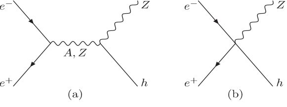
Figure 1: Feynman diagrams for the Higgsstrahlung process $\,e^{+}e^{-}\!\rightarrow Zh$ ,  which include contributions of the relevant dimension-6 operators in Table 1.

In Fig. 1, we summarize the relevant Feynman diagrams for $\,e^{+}e^{-}\!\rightarrow Zh\,$ production, which include possible contributions of the dimension-6 operators in Table 1. Note that only the first diagram (a) has visible contributions, while other diagrams are negligible due to the tiny Higgs-electron Yukawa coupling. This means that the Higgsstrahlung is mainly mediated by $s$-channel gauge boson $Z_{\mu}$ or $A_{\mu}$.  The new physics contributions come from corrections to vertices $\,Z\psi\bar{\psi}\,$ (cf. Sec. 3.3.1), $ZZh$ and $AZh$ (cf. Sec. 3.3.2), as well as $Zh\psi\bar{\psi}$ (cf. Sec. 3.3.3). Among these, the first does not introduce new topology since it contributes an overall factor $\,\delta(g^{2}_{L}\!+\!g^{2}_{R})$  to the SM cross section. This kind of contribution, including field redefinitions which can contribute to the exiting vertices $Z\psi\bar{\psi}$ and $ZZh$, can be treated as a simple rescaling. The others will either modify the tensor structure of the existing vertex or introduce new vertex. We have systematically derived these contributions for the present study. Since the final state consists of only the on-shell particles $Zh$, we can present the results in analytical form. We express the total cross section as a linear combination of the SM contribution and the corrections of dimension-6 operators,

$$\sigma(Zh)\,=\,\left(1+2c^{Z}_{0}\right)\sigma_{\text{sm}}\,+\,\sum_{\,j,V~{}}c_{j}^{V}\sigma_{j}^{V}\,,$$ (39a)

where $$\,c_{0}^{Z}\, \,c_{j}^{V}=c_{j}^{Z},c_{j}^{A}\, \,\sigma_{\text{sm}}\, \,\sigma_{j}^{V}\,$$ is defined in Eq.(22), and are given by Eqs.(21) and (28b). For Eq.(39a), we derive and as follows,

$$\sigma_{\text{sm}} = \frac{(g^{2}_{R}+g^{2}_{L})g_{hZZ}^{2}}{48\pi M_{Z}^{2}\sqrt{s}}\frac{P_{Z}(P_{Z}^{2}+3M_{Z}^{2})}{(s-M^{2}_{Z})^{2}},$$ (39b)

$$\sigma^{Z}_{1} = \frac{(g^{2}_{R}+g^{2}_{L})g_{hZZ}^{2}P_{Z}E_{Z}}{8\pi(s-M^{2}_{Z})(s-M^{2}_{V})},\hskip 51.21495pt\sigma^{A}_{1}\,=\,-\frac{\,g^{2}_{ZZh}(g_{R}+g_{L})e\,}{8\pi(s-M^{2}_{Z})s}E_{Z}P_{Z}\,,~{}~{}~{}~{}~{}$$ (39c)

$$\sigma^{Z}_{2} = -2M_{Z}^{2}\sigma_{\text{sm}}\,,$$ (39d)

$$\sigma^{Z}_{3} = -2\,s\,\sigma_{\text{sm}}\,,\qquad\hskip 93.89409pt\sigma^{A}_{3}\,=\,\frac{\,2(g_{L}\!+\!g_{R})e\,}{g^{2}_{L}\!+\!g^{2}_{R}}{(s\!-\!M^{2}_{Z})}\sigma_{\text{sm}}\,,~{}~{}~{}~{}~{}$$ (39e)

$$\sigma^{\prime}_{Z} = 2\frac{\,g_{L}\delta f_{L}\!+\!g_{R}\delta f_{R}\,}{(g^{2}_{L}\!+\!g^{2}_{R})g_{ZZh}}(s\!-\!M^{2}_{Z})\sigma_{\text{sm}}\,,$$ (39f)

where $(E_{Z},P_{Z})$ denote (energy, $|$momentum$|$) of the final-state $Z$ boson, and the coefficients  ($c^{Z}_{j}$,  $c^{A}_{j}$)  are defined in (21)-(22) as well as (28b). The corrections to fermionic coupling appear in $\,\delta g_{L}\,$ and $\,\delta g_{R}\,$,  as summarized in Sec. 3.3.1. In the last equation (39f), the corrections $\,\delta f_{L}=g_{z}v(c^{(3)}_{L}\!\!+c_{L})/\Lambda^{2}$  and $\,\delta f_{R}=g_{z}vc_{R}/\Lambda^{2}$  are coupling constants of the effective $\,\bar{e}eZh\,$ vertex discussed in (32). Combining everything, we derive the relative corrections to the cross section $\,\sigma(Zh)$ ,

$$\frac{\widetilde{\delta\sigma}}{\sigma} \,\simeq\, 2.34\frac{\delta G_{F}}{G_{F}}+5.51\frac{\delta M_{Z}}{M_{Z}}-0.344\frac{\delta\alpha}{\alpha}-0.0605\frac{c_{H}}{\Lambda_{\mathrm{\scriptscriptstyle TeV}}^{2}}-0.206\frac{c_{T}}{\Lambda_{\mathrm{\scriptscriptstyle TeV}}^{2}}$$ (40)

$$+0.338\frac{c_{WW}}{\Lambda_{\mathrm{\scriptscriptstyle TeV}}^{2}}+0.0122\frac{c_{BB}}{\Lambda_{\mathrm{\scriptscriptstyle TeV}}^{2}}+0.0682\frac{c_{WB}}{\Lambda_{\mathrm{\scriptscriptstyle TeV}}^{2}}+0.0429\frac{c_{HW}}{\Lambda_{\mathrm{\scriptscriptstyle TeV}}^{2}}+0.00315\frac{c_{HB}}{\Lambda_{\mathrm{\scriptscriptstyle TeV}}^{2}}$$

$$+1.02\frac{c^{(3)}_{L}}{\Lambda_{\mathrm{\scriptscriptstyle TeV}}^{2}}+1.02\frac{c_{L}}{\Lambda_{\mathrm{\scriptscriptstyle TeV}}^{2}}-0.755\frac{c_{R}}{\Lambda_{\mathrm{\scriptscriptstyle TeV}}^{2}}.$$

Comparing the above with the Eq.(3.10) of Ref. Craig:2014una , we can see that our coefficient $c_{T}$ is much larger, due to the fact that we use scheme-independent approach instead of the $Z$-scheme. The essential difference between these two approaches is due to the fact that in the $Z$-scheme, $(\alpha,G_{F},M_{Z})$ are fixed to the measured values. To reproduce the $Z$-scheme result from our scheme-independent approach, we can simply set $\,\widetilde{\delta\alpha}\,$ in (34), $\,\widetilde{\delta G_{F}}\,$ in (35), and $\,\widetilde{\delta M_{Z}}\,$ in (36b) to be zero. In this way, the parameter shifts $(\delta\alpha,\delta G_{F},\delta M_{Z})$ can be expressed in terms of dimension-6 operator coefficients. Then, implement these expressions of the parameter shifts into (40). After these operations, the coefficient of $c_{T}$ becomes $-0.0397$, and agrees well with the value $-0.04$ in Ref. Craig:2014una .

4.2.2 WW Fusion: $\bm{e^{+}e^{-}\!\rightarrow\nu\bar{\nu}h}$ at 250 GeV and 350 GeV

The next production mode at the Higgs factory is the $WW$ fusion process as depicted in Fig. 2. Since the cross section $\sigma(\nu\bar{\nu}h)$ at $\sqrt{s}=250$ GeV is about $1/30$ of $\,\sigma(Zh)$  Ruan , the $\sigma(\nu\bar{\nu}h)$ can be measured to a precision of $2.8\%$ at the CEPC CEPC . Although not as precise as the cross section $\sigma(Zh)$ of the Higgsstrahlung process, it can provide complementary constraint on the Higgs coupling with $W$ gauge bosons.

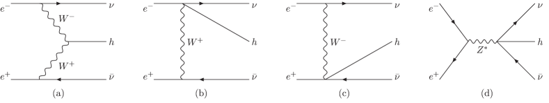
Figure 2: Feynman diagrams for the $WW$ fusion process $\,e^{+}e^{-}\rightarrow h\nu\bar{\nu}$ ,  including contributions of the relevant dimension-6 operators in Table 1.

The new physics contributions can be classified into two categories. The first kind is the contribution to the vertex $WWh$ with fusion topology, as studied in Sec. 3.3.2, which shares the same Feynman diagram Fig. 2(a) as the SM contribution. Corresponding to the coefficients $(c_{0}^{W},c_{1}^{W},c_{2}^{W},c_{3}^{W})$ defined in (25) and (26), we derive the squared $S$-matrix elements,

$$\overline{|\mathcal{M}|^{2}_{0}} = \frac{4g_{Wff}^{4}g^{2}M^{2}_{W}}{(M^{2}_{W}+2p_{1}\!\cdot\!p_{+})^{2}(M^{2}_{W}+2p_{2}\!\cdot\!p_{-})^{2}}(p_{1}\!\cdot\!p_{-})(p_{2}\!\cdot\!p_{+}),$$ (41a)

$$\overline{|\mathcal{M}|^{2}_{1}} = \frac{-2g_{Vff}^{4}g^{2}M^{2}_{W}(p_{1}\!\cdot\!p_{-}\!+p_{2}\!\cdot\!p_{+})}{(M^{2}_{W}\!+\!2p_{1}\!\cdot\!p_{+}\!)^{2}(M^{2}_{W}\!+\!2p_{2}\!\cdot\!p_{-}\!)^{2}}(2p_{1}\!\cdot\!p_{-}p_{2}\!\cdot\!p_{+}\!+2p_{1}\!\cdot\!p_{+}p_{2}\!\cdot\!p_{-}\!-sp_{+}\!\cdot\!p_{-}),~{}~{}~{}~{}~{}~{}$$ (41b)

$$\overline{|\mathcal{M}|^{2}_{2}} \!\!=\!\!\! -2k^{2}_{+}\overline{|\mathcal{M}|^{2}}_{0}=4(p_{2}\!\cdot\!p_{-})\overline{|\mathcal{M}|^{2}_{0}}~{},$$ (41c)

$$\overline{|\mathcal{M}|^{2}_{3}} \!\!=\!\!\! -2k^{2}_{-}\overline{|\mathcal{M}|^{2}_{0}}=4(p_{1}\!\cdot\!p_{+})\overline{|\mathcal{M}|^{2}_{0}}~{},$$ (41d)

where $p_{1}$ and $p_{2}$ denote the momenta of $e^{+}$ and $e^{-}$,  while $p_{+}$ and $p_{-}$ are the momenta of $\nu$ and $\bar{\nu}$,  respectively. The zeroth-order term $\,\overline{|\mathcal{M}|^{2}_{0}}\,$ gives the SM contribution. Only $\,\overline{|\mathcal{M}|^{2}_{1}}\,$ needs to be evaluated independently, the rest are proportional to the zeroth-order result. For the first diagram, its total effect is $\,(1\!+\!2c^{W}_{0})\sigma_{\mathrm{s}m}\!+\sum_{j}c_{j}\sigma_{j}\,$,  with coefficients defined in Eqs. (25) and (26). The second contribution comes from the new vertices in Sec. 3.3.3. Their contribution to the $WW$ fusion is represented by the three new diagrams Fig. 2(b)-(d),

$$\delta|\mathcal{M}_{Wh\ell\bar{\nu}}|^{2} =\, 2|\mathcal{M}_{0}|^{2}\frac{g_{Wh\ell\bar{\nu}}}{\,g_{We\nu}g_{hWW}\,}\left[(k^{2}_{+}\!-M^{2}_{W})+(k^{2}_{-}\!-M^{2}_{W})\right],$$ (42a)

$$\delta|\mathcal{M}_{Zh\nu\bar{\nu}}|^{2} =\, 2|\mathcal{M}_{0}|^{2}\frac{\,(k^{2}_{+}\!-M^{2}_{W})(k^{2}_{-}\!-M^{2}_{W})\,}{s-M_{z}^{2}}\!\left(\!\!-\frac{\,g_{ZeeL}g_{Zh\nu\bar{\nu}}\,}{g_{We\nu}^{2}g_{hWW}}\!\right),~{}~{}~{}~{}~{}$$ (42b)

where $\,k_{\pm}\,$ denotes the momenta of $\,W^{\pm}$. Both contributions come from the interference with the SM contribution $\mathcal{M}_{0}$. For convenience we have denoted the couplings as $\,g_{Wh\ell\bar{\nu}}\equiv\sqrt{2}gvc^{(3)}_{L}/\Lambda^{2}$,  $g_{Zh\nu\bar{\nu}}\equiv g_{z}v(c^{(3)}_{L}\!-c_{L})/\Lambda^{2}$,  $g_{ZeeL}\equiv g_{z}(\frac{1}{2}\!-s^{2}_{w})$,  $g_{We\nu}\equiv g/\!\sqrt{2}$,  and $\,g_{hWW}\equiv g^{2}v/2$ ,  where $\,g_{z}\equiv g/\cos\theta_{w}\,$.  Note that only the left-handed part of the neutral current $\,g_{Zee,L}Z_{\mu}\bar{e}_{L}\gamma^{\mu}e_{L}\,$ in Fig. 2(d) can interfere with the SM contribution $\,\mathcal{M}_{0}$ .  After combining the two contributions, we derive

$$250\,\mbox{GeV}\!:\displaystyle\frac{\widetilde{\delta\sigma}}{\sigma} \,\simeq\, 3.44\frac{\delta G_{F}}{G_{F}}+3.28\frac{\delta M_{Z}}{M_{Z}}-0.442\frac{\delta\alpha}{\alpha}-0.0605\frac{c_{H}}{\Lambda_{\mathrm{\scriptscriptstyle TeV}}^{2}}$$ (43a)

$$+ 0.0515\frac{c_{WW}}{\Lambda_{\mathrm{\scriptscriptstyle TeV}}^{2}}+0.0126\frac{c_{HW}}{\Lambda_{\mathrm{\scriptscriptstyle TeV}}^{2}}-0.159\frac{c^{(3)}_{L}}{\Lambda_{\mathrm{\scriptscriptstyle TeV}}^{2}}+0.0136\frac{c_{L}}{\Lambda_{\mathrm{\scriptscriptstyle TeV}}^{2}},\qquad$$

$$350\,\mbox{GeV}\!:\displaystyle\frac{\widetilde{\delta\sigma}}{\sigma} \simeq\, 3.52\frac{\delta G_{F}}{G_{F}}+3.89\frac{\delta M_{Z}}{M_{Z}}-0.523\frac{\delta\alpha}{\alpha}-0.0605\frac{c_{H}}{\Lambda_{\mathrm{\scriptscriptstyle TeV}}^{2}}$$ (43b)

$$+ 0.0575\frac{c_{WW}}{\Lambda_{\mathrm{\scriptscriptstyle TeV}}^{2}}+0.0188\frac{c_{HW}}{\Lambda_{\mathrm{\scriptscriptstyle TeV}}^{2}}-0.226\frac{c^{(3)}_{L}}{\Lambda_{\mathrm{\scriptscriptstyle TeV}}^{2}}+0.00918\frac{c_{L}}{\Lambda_{\mathrm{\scriptscriptstyle TeV}}^{2}},$$

for $\,\sqrt{s}=250\,\mbox{GeV}$ and 350 GeV, respectively. At $\,\sqrt{s}=350$ GeV, we see that the Higgs production cross section through $WW$ fusion has sizable increase, leading to a better measurement of $\,\sigma(\nu\bar{\nu}h)$ .

4.2.3 Higgs Decay into $Z$ Boson Pair

For Higgs decay into the $Z$ boson pair, at least one of them must be off-shell. The decay width can be computed via the corresponding three-body decay process, $\,h\rightarrow ZZ^{*}\rightarrow Zf\bar{f}$ .  In addition, the double off-shell process $\,h\rightarrow Z^{*}Z^{*}$  still contributes $25\%$ of the partial width and thus should be included via the four-body decay process, $\,h\rightarrow Z^{*}Z^{*}\rightarrow f_{1}\bar{f}_{1}f_{2}\bar{f}_{2}$ .  We compute the new physics contributions to the Higgs partial width by using FeynRules FeynRules and MadGraph5 Mad5 . With these, we derive the following expression,

$$\frac{\,\widetilde{\delta\Gamma}\,}{\Gamma} \simeq 3.42\frac{\delta G_{F}}{G_{F}}-5.44\frac{\delta M_{Z}}{M_{Z}}-0.420\frac{\delta\alpha}{\alpha}-0.0605\frac{c_{H}}{\Lambda_{\mathrm{\scriptscriptstyle TeV}}^{2}}+0.190\frac{c_{T}}{\Lambda_{\mathrm{\scriptscriptstyle TeV}}^{2}}$$ (44)

$$-0.0968\frac{c_{WW}}{\Lambda_{\mathrm{\scriptscriptstyle TeV}}^{2}}-0.0255\frac{c_{BB}}{\Lambda_{\mathrm{\scriptscriptstyle TeV}}^{2}}-0.0579\frac{c_{WB}}{\Lambda_{\mathrm{\scriptscriptstyle TeV}}^{2}}+0.0131\frac{c_{HW}}{\Lambda_{\mathrm{\scriptscriptstyle TeV}}^{2}}+0.0144\frac{c_{HB}}{\Lambda_{\mathrm{\scriptscriptstyle TeV}}^{2}}$$

$$+0.0410\frac{c^{(3)}_{L}}{\Lambda_{\mathrm{\scriptscriptstyle TeV}}^{2}}-0.0112\frac{c_{L}}{\Lambda_{\mathrm{\scriptscriptstyle TeV}}^{2}}-0.00957\frac{c_{R}}{\Lambda_{\mathrm{\scriptscriptstyle TeV}}^{2}}$$

$$+0.101\frac{c^{(3)}_{L,q}}{\Lambda_{\mathrm{\scriptscriptstyle TeV}}^{2}}+0.0269\frac{c_{L,q}}{\Lambda_{\mathrm{\scriptscriptstyle TeV}}^{2}}+0.0128\frac{c_{R,u}}{\Lambda_{\mathrm{\scriptscriptstyle TeV}}^{2}}-0.00957\frac{c_{R,d}}{\Lambda_{\mathrm{\scriptscriptstyle TeV}}^{2}}.$$

The CEPC detector simulations CEPC show that this decay branching fraction can be measured to the precision of $4.3\%$ .

4.2.4 Higgs Decay into $W$ Boson Pair

The analysis of this process is similar to that of $\,h\rightarrow ZZ$ .  We use FeynRules FeynRules and MadGraph5 Mad5 to numerically compute the new physics contributions to $h\rightarrow WW^{*},W^{*}W^{*}$ with 3-body and 4-body final states. Altogether, we derive the contributions of the relevant dimension-6 operators to the following,

$$\frac{\widetilde{\delta\Gamma}}{\Gamma} \simeq 1.64\frac{\delta G_{F}}{G_{F}}-10.1\frac{\delta M_{Z}}{M_{Z}}+1.36\frac{\delta\alpha}{\alpha}-0.0605\frac{c_{H}}{\Lambda_{\mathrm{\scriptscriptstyle TeV}}^{2}}$$ (45)

$$-0.233\frac{c_{WW}}{\Lambda_{\mathrm{\scriptscriptstyle TeV}}^{2}}+0.0225\frac{c_{HW}}{\Lambda_{\mathrm{\scriptscriptstyle TeV}}^{2}}+0.0479\frac{c^{(3)}_{L}}{\Lambda_{\mathrm{\scriptscriptstyle TeV}}^{2}}+0.0968\frac{c^{(3)}_{L,q}}{\Lambda_{\mathrm{\scriptscriptstyle TeV}}^{2}}.$$

The branching fraction of $\,h\rightarrow WW\,$ can be measured with to $\,1.5\%\,$ accuracy at the CEPC CEPC . Note that this channel is measured with better precision than $\,h\rightarrow ZZ$ .  This is because $W$ is lighter than $Z$, and hence the $\,WW\,$ channel has much larger branching fraction than the $ZZ$ channel. This difference in decay rates leads to different precisions which are mainly dominated by statistical fluctuations.

4.2.5 Other Decay Channels

The remaining Higgs decay channels can be divided into two major classes: one with fermionic decay products and the other with massless gauge bosons (photons or gluons). The first class occurs at tree-level, while the second class arises from one-loop level. Both receive contributions from the Higgs field redefinition (8),

$$\frac{\,\delta\Gamma\,}{\Gamma}\,=\,-0.0605\frac{c_{H}}{\,\Lambda_{\mathrm{\scriptscriptstyle TeV}}^{2}\,}\,,$$ (46)

which is the only contribution to fermionic decays. The vertex $\,f\bar{f}h\,$ comes from Yukawa interaction which flips chirality and is not affected by either the dimension-6 operators in Table 1 or the EW parameters mentioned earlier. On the other hand, the decay into photons has extra contributions. For fermion loop, it is affected by the photon field redefinition (11b) only. For bosonic $W$-loop, the new physics effects come from $W$-mass correction (10) and the photon field redefinition (11b). Note that the corrections of $W$-field redefinition to the vertex and mass should cancel with each other. Since the EW parameters are involved in bosonic decay, their shifts $(\delta\alpha,\,\delta G_{F},\,\delta M_{Z})$ should also appear. Note that $\,h\rightarrow gg\,$ only has fermionic contributions.

Furthermore, dimension-6 operators induce direct coupling of the Higgs field $h$ with photons or gluons, as shown in Eqs. (29) and (30), respectively. Thus, we derive the following $hAA$ and $hgg$ couplings,

$$\mathcal{M}_{hAA} = \frac{4}{\,v\,}\delta Z_{A}f^{\mu\nu}\llbracket p_{1},p_{2}\rrbracket\epsilon_{1\mu}\epsilon_{2\nu}\,,~{}~{}~{}~{}~{}$$ (47a)

$$\mathcal{M}_{hgg} = \frac{4v}{\,\Lambda^{2}\,}g_{s}^{2}c_{g}f^{\mu\nu}\llbracket p_{1},p_{2}\rrbracket\,\delta_{ab}\,\epsilon_{1\mu}\epsilon_{2\nu}\,.$$ (47b)

We may compare them with the corresponding SM-loop results,

$$\mathcal{M}_{hAA}^{\text{sm}} \,=\, \frac{e^{2}}{\,8\pi^{2}v\,}\left(F_{W}+\sum N_{c}Q_{f}^{2}F_{f}\right)\!f^{\mu\nu}\llbracket p_{1},p_{2}\rrbracket\epsilon_{1\mu}\epsilon_{2\nu},$$ (48a)

$$\mathcal{M}_{hgg}^{\text{sm}} \,=\, \frac{\alpha_{s}}{\,4\pi v\,}F_{f}f^{\mu\nu}\llbracket p_{1},p_{2}\rrbracket\,\delta_{ab}\,\epsilon_{1\mu}\epsilon_{2\nu},$$ (48d)

$$F_{W}\equiv~{}2+3\tau_{W}^{-1}\left[1+(2-\tau_{W}^{-1})f(\tau_{W})\right]\!,$$

$$F_{f}~{}\equiv\,-2\tau_{f}^{-1}\left[1+(1-\tau_{f}^{-1})f(\tau_{f})\right]\!,$$

where $\,\tau_{j}\equiv{M_{h}^{2}}/{(4M_{j}^{2})}$  and $\,f(\tau_{j})\equiv(\arcsin\!\sqrt{\tau_{j}})^{2}\,$,  with $\,j=W,t$.  Combining everything together, we derive the total corrections,

$$\frac{\,\delta\Gamma_{AA}\,}{\Gamma_{AA}} = 0.997\frac{\delta G_{F}}{G_{F}}+2\frac{\delta\alpha}{\alpha}-0.0218\frac{\delta M_{Z}}{M_{Z}}-0.0605\frac{c_{H}}{\,\Lambda_{\mathrm{\scriptscriptstyle TeV}}^{2}}+5.91\frac{\,c_{WW}\!-\!c_{WB}\!+\!c_{BB}\,}{\Lambda_{\mathrm{\scriptscriptstyle TeV}}^{2}},~{}~{}~{}~{}~{}~{}\qquad$$ (49a)

$$\frac{\,\delta\Gamma_{gg}\,}{\Gamma_{gg}} = \frac{\delta G_{F}}{G_{F}}-0.0605\frac{c_{H}}{\,\Lambda_{\mathrm{\scriptscriptstyle TeV}}^{2}}-55.2\frac{c_{g}}{\,\Lambda_{\mathrm{\scriptscriptstyle TeV}}^{2}}\,,$$ (49b)

for $\,\Gamma_{AA}\,$ and $\,\Gamma_{gg}$ ,  respectively. We note that the coefficients of the last terms in both (49a) and (49b) come from the interference between the SM prediction (48) and the contribution (47) by dimension-6 operators. Although the SM predictions of $\,h\rightarrow gg\,$ and $\,h\rightarrow\gamma\gamma\,$ arise from loop-level and are expected to be of the same order as that of dimension-6 operators, it is well justified to make expansion up to the linear terms of $\,c_{g}$  and $\,(c_{WW},c_{WB},c_{BB})$.  This is because the current LHC data constrain the deviations from the SM predictions within about 20% at $2\sigma$ level LHC-fit , and the future Higgs factory sensitivities to such deviations are even much smaller (Table 2 in Sec. 4.3 and Fig. 5 in Appendix 5). Hence, the dimension-6 contributions can be well treated as small perturbations up to the linear order.

4.3 Probing New Physics Scales at Higgs Factory

As discussed in Sec. 4.1 and Sec. 4.2, the dimension-6 effective operators can modify both EW precision observables (EWPO) and Higgs observables (HO). The EWPO have been precisely measured at the LEP and Tevatron with high precision, while the HO can be measured at the future Higgs factory under planning. Currently, there are three major candidates of Higgs factory, CEPC CEPC , FCC-ee FCC-ee , and ILC ILC , which can run at the collision energies around $240-250$ GeV. They can measure the Higgs production cross sections and decay branching fractions with precisions at percentage level. This provides important means to indirectly probe the scales of new physics. In the following, we study how the EWPO and HO can probe the new physics scales via effective dimension-6 operators and the interplay with each other.

For convenience, we first summarize the inputs for our analysis in Table 2. Since the EWPO have already been measured, we list both their central values and relative errors. These four observables are the most precisely measured ones. Especially, the fine-structure constant $\alpha$ is measured with unprecedented precision of $\,\delta\alpha/\alpha=3.29\!\times\!10^{-10}$,  much better than all the others. According to its expression (34), one degrees of freedom can be effectively eliminated. This is also true for the Fermi constant $\,G_{F}$ ,  whose precision $\,\delta G_{F}/G_{F}=5.14\!\times\!10^{-7}$  is just next to that of $\,\alpha$ .

Table 2: Inputs used to constrain the new physics scales of the dimension-6 operators. The electroweak precision observables in the first four rows are taken from PDG PDG14 , and the estimated precisions of Higgs measurements (68% C.L.) are given by the CEPC detector simulations CEPC . For the $WW$ fusion cross section $\sigma[\nu\bar{\nu}h]_{350\text{GeV}}$ at $\sqrt{s}=350$ GeV, we adopt the FCC-ee (TLEP) estimation FCC-ee for illustration. For the “Measurements” entry, the number inside the parentheses stands for experimental uncertainty.

Observables	Measurements	Relative Error	SM Prediction
$M_{Z}$	91.1876(21) GeV	$2.3\times 10^{-5}$	–
$M_{W}$	80.385(15) GeV	$1.87\times 10^{-4}$	–
$G_{F}$	$1.1663787(6)\!\times\!10^{-5}\mbox{GeV}^{-2}$	$5.14\!\times\!10^{-7}$	–
$\alpha$	$7.2973525698(24)\!\times\!10^{-3}$	$3.29\!\times\!10^{-10}$	–
$\sigma[Zh]$	–	0.50%	–
$\sigma[\nu\bar{\nu}h]$	–	2.86%	–
$\sigma[\nu\bar{\nu}h]_{350\text{GeV}}$	–	0.75%	–
$\text{Br}[WW]$	–	1.2%	22.5%
$\text{Br}[ZZ]$	–	4.3%	2.77%
$\text{Br}[bb]$	–	0.54%	58.1%
$\text{Br}[cc]$	–	2.5%	2.10%
$\text{Br}[gg]$	–	1.4%	7.40%
$\text{Br}[\tau\tau]$	–	1.1%	6.64%
$\text{Br}[\gamma\gamma]$	–	9.0%	0.243%
$\text{Br}[\mu\mu]$	–	17%	0.023%

For the Higgs observables, Table 2 summarizes the estimated precisions at the CEPC CEPC . The production cross sections and branching fractions are independent of each other. Nevertheless, the decay widths (44)-(45) for Higgs decays into $ZZ$ and $WW$ bosons cannot be directly used to compare with the branching fraction precisions in Table 2. The decay width for a specific channel competes with all other channels, so its corresponding branching fraction is given by $\,\text{Br}_{j}\equiv\Gamma_{j}/\Gamma$,  where $\,\Gamma\equiv\sum_{k}\Gamma_{k}$  is the total decay width. Each partial width can be expressed as $\,\Gamma_{j}\equiv\Gamma^{(r)}_{j}(1+\delta\Gamma_{j}/\Gamma_{j})$  with $\,\delta\Gamma_{j}\,$ denoting the deviation from the reference point. When expanded to linear order, the decay branching fraction becomes,

$$\text{Br}_{j}~{}\simeq~{}\text{Br}^{(r)}_{j}\!\left[1+\left(1-\text{Br}^{(r)}_{j}\right)\!\frac{\,\delta\Gamma_{j}\,}{\Gamma_{j}}-\sum_{k\neq j}\text{Br}^{(r)}_{k}\frac{\,\delta\Gamma_{k}\,}{\Gamma_{k}}\right]\!.$$ (50)

The corrections to Higgs partial width affect not only its own branching fraction, but also all the others. Eq.(50) shows that for the branching fraction $\,\text{Br}_{j}$,  the contribution due to its own channel is modulated by $\,1\!-\text{Br}^{(r)}_{j}$,  while other channels by the corresponding $\,\text{Br}^{(r)}_{k}$.  Since the reference value is around the SM prediction, $\,\text{Br}^{(r)}_{j}\!\approx\text{Br}^{\text{sm}}_{j}$,  the modulation is essentially controlled by the SM predictions. In this way, the precision measurements of branching fractions at CEPC will constrain the new physics scales via $\,\delta\Gamma_{j}\,$ term and $\,\delta\Gamma_{k}\,$ term.

The observables in Table 2 can be used to constrain the electroweak parameters $(\delta\alpha$, $\delta G_{F}$, $\delta M_{Z})$ and the coefficients of dimension-6 operators simultaneously. This can be achieved by the so-called $\chi^{2}$ fit technique. As described in Appendix B, the $\chi^{2}$ function sums over all experimental observables $\,\mathcal{O}_{j}$ ,

$$\chi^{2}\!\left(\delta\alpha,\delta G_{F},\delta M_{Z},\frac{c_{i}}{\Lambda^{2}}\right)~{}=~{}\sum_{j}\left[\frac{\,\mathcal{O}^{\mathrm{th}}_{j}\!\left(\delta\alpha,\delta G_{F},\delta M_{Z},\frac{c_{i}}{\Lambda^{2}}\right)-\mathcal{O}^{\mathrm{exp}}_{j}\,}{\Delta\mathcal{O}_{j}}\right]^{\!2},~{}~{}~{}~{}~{}$$ (51)

where the theoretical predictions are functions of the fitting parameters. The $\chi^{2}$ function reaches its minimal value at the best fit values of $(\delta\alpha,\delta G_{F},\delta M_{Z})$ and $c_{i}/\Lambda^{2}$. Using the linear $\chi^{2}$ fitting method shown in Appendix  B, we can perform this fit analytically with the package BSMfitter BSMfitter . As usual, for simplicity, we will consider only one dimension-6 effective operator to be nonzero during each fit, and turn off the others. Thus, each fit will deal with only four fitting parameters, $(\delta\alpha,\delta G_{F},\delta M_{Z})$ and one dimension-6 coefficient $\,c_{i}/\Lambda^{2}\,$.

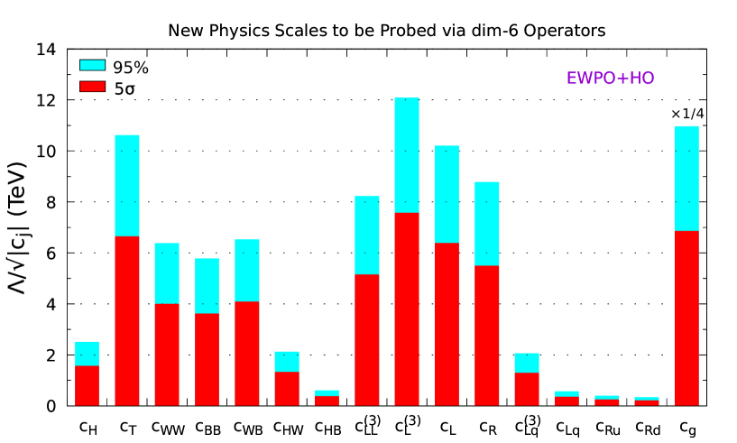
Figure 3: The 95% exclusion limits (blue) and $5\sigma$ discovery sensitivities (red) to the new physics scales $\,\Lambda/\!\sqrt{|c_{j}|}\,$ by combining the current electroweak precision observables ($\alpha,\,G_{F},\,M_{Z},\,M_{W}$) PDG14 and the future Higgs observables (Table 2) at the Higgs factory CEPC (250 GeV) CEPC with a projected luminosity of  5 ab^-1. In the last column for $\mathcal{O}_{g}$, we have rescaled its height by a factor $1/4$ to fit the plot, so its actual reach is $\,\Lambda/\!\sqrt{|c_{g}|}=43.8\,$TeV.

In Fig. 3, we present the lower limit on the new physics scale of each dimension-6 operator by combining the existing electroweak precision measurements and future Higgs measurements at the CEPC with $\sqrt{s}=250\,\mbox{GeV}$. We see that it can probe the new physics scales up to about $12\,\mbox{TeV}$ for $\mathcal{O}^{(3)}_{L}$ at 95% C.L.

For the operators listed in Table 1, ($\mathcal{O}_{T}$, $\mathcal{O}^{(3)}_{LL}$, $\mathcal{O}^{(3)}_{L}$, $\mathcal{O}_{L,R}$, $\mathcal{O}_{g}$) are among the first group to be sensitively probed. Roughly speaking, they can be probed up to the new physics scales $\,(8-10)\,\mbox{TeV}$.  The second group consists ($\mathcal{O}_{H}$, $\mathcal{O}_{WW}$, $\mathcal{O}_{BB}$, $\mathcal{O}_{WB}$, $\mathcal{O}_{HW}$, $\mathcal{O}^{(3)}_{Lq}$), which can be probed up to the scales $\,(2-5)\,\mbox{TeV}$.  The others operators, ($\mathcal{O}_{HB}$, $\mathcal{O}_{Lq}$, $\mathcal{O}_{Ru}$, $\mathcal{O}_{Rd}$), cannot be probed above the  1 TeV scale. We note that the strong constraint on $\mathcal{O}_{T}$ mainly comes from the $W$ boson mass $M_{W}$.  Including electroweak precision observables can significantly improve the probe of new physics scales, as we will fully elaborate in following Sec. 4.4 and Sec. 4.5. The remaining constraints come from measuring the Higgs production and decay rates, most of which is provided by the Higgsstrahlung process. For the gluonic operator $\,\mathcal{O}_{g}$,  its constraint is mainly given by the branching fraction of $\,h\rightarrow gg\,$ which is the only relevant channel here. Although this is not the major Higgs decay channel, with the SM prediction $\,\text{Br}[gg]=7.4\%$,  it can put severe constraint on the scale of $\,\mathcal{O}_{g}$,  as high as about 43.8 TeV (cf. Fig. 3). Since in the SM the Higgs coupling with gluons arises at one-loop level and the dimension-6 operator $\,\mathcal{O}_{g}$  contributes to this coupling at tree-level, so the scale of $\,\mathcal{O}_{g}$  has to be high enough to suppress the deviation from the SM loop prediction. This is expected since the operator $\,\mathcal{O}_{g}$  may well be induced from loop-level in a given underlying theory and thus its coefficient $\,c_{g}\,$ will be suppressed by the corresponding loop-factor.

Note that Fig. 3 contains more fermionic operators than listed in Table 1 since quark and lepton can provide different contributions. For a specific operator, we assume the same operator coefficient for the three generations of fermions. Consequently, each of the operators involving left-handed fermions, ($\mathcal{O}^{(3)}_{LL},\,\mathcal{O}^{(3)}_{L},\,\mathcal{O}_{L}$), has two copies, one for leptons and the other for quarks (with extra subscript “$q$”). On the other hand, the operator $\,\mathcal{O}_{R}\,$ that contains the right-handed fermions has three copies, one for charged leptons and the other two for quarks (with subscripts “$u$” for up- and “$d$ ” for down-type quarks). We can see that leptonic operators are generally better constrained than those of quarks, since the former can enter the most precisely measured Higgsstrahlung process, and the latter can only be constrained by Higgs decays into $WW$ and $ZZ$ with limited branching fractions and statistics. Although the Higgs decay mode $\,h\rightarrow b\bar{b}\,$ has the largest branching fraction, it is not connected to the fermionic operators shown in Table 1.

Table 3: New physics scales $\Lambda/\!\sqrt{|c_{j}|}$ (in TeV) which can be probed by combining the current electroweak precision tests on ($\alpha,G_{F},M_{Z},M_{W}$) PDG14 and the future Higgs measurements on ($\sigma(Zh)$, $\sigma(\nu\bar{\nu}h)$, and branching fractions) at the Higgs factory CEPC (250 GeV) CEPC with a projected luminosity of 5 ab^-1. The sensitivities are presented as the $95\%$ exclusions (first row) and the $5\,\sigma$ discoveries (second row), respectively.

$\mathcal{O}_{H}$	$\mathcal{O}_{T}$	$\mathcal{O}_{WW}$	$\mathcal{O}_{BB}$	$\mathcal{O}_{WB}$	$\mathcal{O}_{HW}$	$\mathcal{O}_{HB}$	$\mathcal{O}^{(3)}_{LL}$	$\mathcal{O}^{(3)}_{L}$	$\mathcal{O}_{L}$	$\mathcal{O}_{R}$	$\mathcal{O}^{(3)}_{L,q}$	$\mathcal{O}_{L,q}$	$\mathcal{O}_{R,u}$	$\mathcal{O}_{R,d}$	$\mathcal{O}_{g}$
2.5	10.6	6.38	5.78	6.53	2.12	0.604	8.23	12.1	10.2	8.78	2.06	0.568	0.393	0.339	43.8
1.57	6.65	4.00	3.62	4.09	1.33	0.378	5.15	7.57	6.39	5.49	1.29	0.356	0.246	0.212	27.4

For clarity, in Table 3, we further present the numerical limits of Fig. 3 at both 95% and $5\sigma$ confidence levels. The 95% limit corresponds to the exclusion reach, while $5\sigma$ limits gives the discovery reach. Since the results are obtained after reducing to one-dimensional Gaussian distribution by marginalization (see Appendix B for detail), the value of the $5\sigma$ reach on the new physics scale equals 39% of the corresponding 95% confidence limit.

Note that these results are obtained with all Higgs observables to be measured at $\sqrt{s}=250\,\mbox{GeV}$. If the collision energy is upgraded to $350\,\mbox{GeV}$, the cross section of the $WW$ fusion process for Higgs production will increase significantly. This can help to enhance the sensitivity to the scale of $\,\mathcal{O}_{H}\,$ by about  10%,  as will be shown in the first column of Table 6, while the others remain the same.

4.4 Combining with Electroweak Precision Observables

For comparison, we note that the $Z$-scheme is adopted in the recent studies Craig:2014una and Ellis:2015sca , where the latter also invokes the $W$ mass measurement at a Higgs factory. In this scheme, not all the electroweak parameters, especially the most precisely measured ones ($\alpha,G_{F},M_{Z}$), were included in their analysis. After incorporating the electroweak precision measurements, including also $M_{W}$,  the reach of new physics scales Ellis:2015sca becomes higher than the one with the $\,\sigma(Zh)\,$ constraints alone Craig:2014una . Although the $\,M_{W}\,$ measurement is also used in Ellis:2015sca , its interplay with $M_{Z}$ could not be studied within the $Z$-scheme. In this subsection, we first study the role of electroweak precision observables (EWPO) with the current data PDG14 . We will further analyze the interplay of including a significantly improved $M_{W}$ measurement in Sec. 4.5.

Among the existing EWPO, the most precisely measured observables are $\alpha$, $G_{F}$, and $M_{Z}$, in the order of their relative uncertainties, as shown in Table 2. Even the least precise one, $M_{Z}$, is much better measured than the other mass $M_{W}$ by about one order of magnitude. This hierarchical structure in the relative uncertainties makes it appropriate to treat $(\alpha,G_{F},M_{Z})$ as inputs to fix the electroweak parameters ($g,g^{\prime},v$), and implement the $M_{W}$ measurement into the fit. As we discussed in Sec. 4.2.1, this is equivalent to setting $\,(\widetilde{\delta\alpha},\,\widetilde{\delta G_{F}},\,\widetilde{\delta M_{Z}})=0$ ,  from which $(\delta\alpha,\delta G_{F},\delta M_{Z})$ can be solved in terms of dimension-6 operator contributions. With these extra constraints (which is exactly the definition of $Z$-scheme) implemented into (36a), we derive the $W$ mass correction as

$$\frac{\widetilde{\delta M_{W}}}{M_{W}}\,=~{}0.0414\frac{c_{T}}{\Lambda_{\mathrm{\scriptscriptstyle TeV}}^{2}}-0.00964\frac{c_{WB}}{\Lambda_{\mathrm{\scriptscriptstyle TeV}}^{2}}-0.0223\frac{c^{(3)}_{LL}}{\Lambda_{\mathrm{\scriptscriptstyle TeV}}^{2}}+0.0223\frac{c^{(3)}_{L}}{\Lambda_{\mathrm{\scriptscriptstyle TeV}}^{2}}\,,~{}~{}~{}~{}~{}$$ (52)

which is a function of the coefficients of dimension-6 operators alone. In Eq. (52), even though the coefficients of the $\,c_{T}\,$ and $\,c_{L}\,$ terms are not sizable, after imposing the experimental data $\,M_{W}=80.385\!\times\!(1\pm 1.87\!\times\!10^{-4})$ GeV (which is much more precise than the Higgs observables to be measured at the future Higgs factory), we can estimate the limit on the new physics scale to be $\,\Lambda/\!\sqrt{|c_{T}|}>14.9\,(7.59)\,$TeV at $1\sigma$ (95% C.L.). This demonstrates significant improvement of the new physics reach from the precision measurements of the EWPO. After further including the CEPC measurement of $\sigma(Zh)$, we find the improved limit, $\,\Lambda/\!\sqrt{|c_{T}|}>10.6\,$TeV at 95% C.L., as shown in Table 4.

Table 4: Impacts of adding the current electroweak precision observables ($\alpha,G_{F},M_{Z},M_{W}$) PDG14 on probing the new physics scales $\,\Lambda/\!\sqrt{|c_{j}|}$ (in TeV) at 95% C.L. The limits in the first row are obtained from $\sigma(Zh)$ to be measured at the CEPC CEPC only. The limits in the second row are given by combining with the current $M_{W}$ measurement plus $\sigma(Zh)$.  Finally, the third row presents the limits by including the current measurements of $(\alpha,G_{F},M_{Z})$ altogether. In the first two rows, $(\alpha,G_{F},M_{Z})$ are fixed to their experimental central values as in the $Z$-scheme, while the third row adopts the scheme-independent approach by allowing all electroweak parameters to freely vary in each fit. We label the entries of most significant improvements in red color with an underscore.

$\mathcal{O}_{H}$	$\mathcal{O}_{T}$	$\mathcal{O}_{WW}$	$\mathcal{O}_{BB}$	$\mathcal{O}_{WB}$	$\mathcal{O}_{HW}$	$\mathcal{O}_{HB}$	$\mathcal{O}^{(3)}_{LL}$	$\mathcal{O}^{(3)}_{L}$	$\mathcal{O}_{L}$	$\mathcal{O}_{R}$
2.48	2.01	4.83	0.89	1.86	2.09	0.567	5.38	11.6	10.2	8.78
2.48	10.6	4.83	0.89	5.16	2.09	0.567	8.22	12.1	10.2	8.78
2.48	10.6	4.83	0.875	5.12	2.09	0.567	8.15	12.1	10.2	8.78

In Table 4, the first two rows are essentially $Z$-scheme approach with $(\alpha,G_{F},M_{Z})$ fixed. Here we see whether including the current $M_{W}$ measurement or not leads to significant difference. The change appears in the probed new physics scales of the four operators $\mathcal{O}_{T}$, $\mathcal{O}_{WB}$, $\mathcal{O}^{(3)}_{LL}$, and $\mathcal{O}^{(3)}_{L}$,  which are involved in the $Z$-scheme correction (52). For them, the most significant changes come from $\mathcal{O}_{T}$ and $\mathcal{O}_{WB}$, since the reaches of the corresponding new physics scales are enhanced by about a factor of $5$ and $3$, respectively. It shows that for $\mathcal{O}_{T}$, the probe of its new physics scale is enhanced from $2.01\,\mbox{TeV}$ to $10.6\,\mbox{TeV}$ once $M_{W}$ measurement is included. Setting the most precisely measured observables $(\alpha,G_{F},M_{Z})$ be their experimental central values is equivalent to fixing the electroweak observables. This justifies the $Z$-scheme approach when the precisions of $(\alpha,G_{F},\,M_{Z})$ are much higher than the others. In Sec. 4.5, we will further analyze how the situation changes when the precisions of $M_{Z}$ and $M_{W}$ measurements become comparable with each other.

4.5 Enhanced Sensitivity from CEPC Measurements of ${W/Z}$ Masses

Lepton colliders such as the CEPC, FCC-ee and ILC can also make $Z$-pole measurements, which are necessary for calibrations at the initial stage of running the machine. To make full use of the $Z$-pole running, we can utilize the $Z$-pole data to further enhance the indirect probe of new physics scales. The most significant improvements include the weak boson masses $M_{Z}$ and $M_{W}$, as shown in Table 5 for the CEPC.

Table 5: Projected precisions (68% C.L.) of $Z$ and $W$ mass measurements at the CEPC CEPC ; Zpole .

Observables	Relative Error	Absolute Error
$M_{Z}$	$(0.55-1.1)\!\times\!10^{-5}$	$(0.5-1)$ MeV
$M_{W}$	$(3.7-6.2)\!\times\!10^{-5}$	$(3-5)$ MeV

In comparison with the existing precision data shown in the first block of Table 2, we see that the uncertainties of $\,M_{Z}\,$ and $\,M_{W}\,$ can be further improved by a factor of $\,2-4\,$ and $\,3-5$,  respectively. Since the constraints from current precision measurements are already rather sensitive, we can expect more significant enhancements by imposing the CEPC measurements. A rough estimate leads us to expect that the sensitivity to new physics scales could be doubled for operators $\mathcal{O}_{T}$ and $\mathcal{O}_{L}$,  reaching about $20\,\mbox{TeV}$.

In Table 6, we quantitatively analyze the impacts of imposing the $Z$-pole measurements of $M_{Z}$ and $M_{W}$ at the CEPC. In the following analysis, we implement the relative errors $\,8.25\!\times\!10^{-6}\,$ for $M_{Z}$ and $\,3.7\!\times\!10^{-5}\,$ for $M_{W}$ as an illustration. Here, we see that the relative errors of $M_{Z}$ and $M_{W}$ become comparable with each other. Including $M_{Z}$ alone makes no significant improvement. As we demonstrated in Table 4 and the related discussions, the effect of inputting the precision data $M_{Z}$ is to fix one of the three electroweak parameters. Adding a better measurement of $M_{Z}$ would not change this picture, except to further enhance it. On the other hand, imposing the CEPC measurement of $M_{W}$ alone can significantly improve the reach of new physics scales. This increases the sensitivities to the scales of $\mathcal{O}_{T}$, $\mathcal{O}_{WB}$, $\mathcal{O}_{L}$, and $\mathcal{O}^{(3)}_{LL}$ by about a factor of two, as shown in the third row of Table 6. This result is consistent with what we have observed in Table 4. A new point is that further imposing the CEPC measurement of $M_{Z}$, after imposing $M_{W}$,  can introduce extra improvement, although adding the CEPC measurement of $M_{Z}$ alone cannot. It demonstrates the fact that when the precisions of $M_{Z}$ and $M_{W}$ are comparable with each other, it is no longer appropriate to just pick up the three observables to fix the three electroweak variables. In other words, $Z$-scheme is a good approximation when the relative errors of $(\alpha,G_{F},M_{Z})$ are all much smaller than the others. This appears no longer the case at future lepton colliders. Here, we use the projected CEPC sensitivities to $M_{Z}$ and $M_{W}$ CEPC ; Zpole as an illustration, and we have demonstrated that the present scheme-independent approach is a more general-purpose method. In the conventional $Z$-scheme, $M_{Z}$ is commonly fixed to the experimental central value, so that the above improvement is impossible.

Table 6: Impacts of the projected $M_{Z}$ and $M_{W}$ measurements at CEPC CEPC ; Zpole on the reach of new physics scale $\Lambda/\!\sqrt{|c_{j}|}$ (in TeV) at 95% C.L. The Higgs observables (including $\sigma(\nu\bar{\nu}h)$ at 350 GeV) and the existing electroweak precision observables (Table 2) are always included in each row. The differences among the four rows arise from whether taking into account the measurements of $M_{Z}$ and $M_{W}$ (Table 5) or not. The second (third) row contains the measurement of $M_{Z}$ ($M_{W}$) alone, while the first (last) row contains none (both) of them. We mark the entries of the most significant improvements from $M_{Z}$ and/or $M_{W}$ measurements in red color with an underscore.

$\mathcal{O}_{H}$	$\mathcal{O}_{T}$	$\mathcal{O}_{WW}$	$\mathcal{O}_{BB}$	$\mathcal{O}_{WB}$	$\mathcal{O}_{HW}$	$\mathcal{O}_{HB}$	$\mathcal{O}^{(3)}_{LL}$	$\mathcal{O}^{(3)}_{L}$	$\mathcal{O}_{L}$	$\mathcal{O}_{R}$	$\mathcal{O}^{(3)}_{L,q}$	$\mathcal{O}_{L,q}$	$\mathcal{O}_{R,u}$	$\mathcal{O}_{R,d}$	$\mathcal{O}_{g}$
2.74	10.6	6.38	5.78	6.53	2.16	0.604	8.58	12.1	10.2	8.78	2.06	0.568	0.393	0.339	43.8
2.74	10.7	6.38	5.78	6.54	2.16	0.604	8.62	12.1	10.2	8.78	2.06	0.568	0.393	0.339	43.8
2.74	21.0	6.38	5.78	10.4	2.16	0.604	15.5	16.4	10.2	8.78	2.06	0.568	0.393	0.339	43.8
2.74	23.7	6.38	5.78	11.6	2.16	0.604	17.4	18.1	10.2	8.78	2.06	0.568	0.393	0.339	43.8

4.6 Enhancement from $Z$-Pole Observables at CEPC

In addition to the mass measurements of $W$ and $Z$, CEPC can also measure the $Z$ boson lineshape at the $Z$-pole, $\sqrt{s}=M_{Z}$ .  Currently, there are six observables that have been simulated at CEPC CEPC ; Zpole . For convenience, we summarize them in Table 7, in the order of their relative precisions.

Table 7: Projected precisions (68% C.L.) of $Z$-pole measurements at the CEPC CEPC ; Zpole .

Observables	Relative Error
$N_{\nu}$	$1.8\times 10^{-3}$
$A_{FB}(b)$	$1.5\times 10^{-3}$
$R_{b}$	$8\times 10^{-4}$
$R_{\mu}$	$5\times 10^{-4}$
$R_{\tau}$	$5\times 10^{-4}$
$\sin^{2}\theta_{W}$	$1\times 10^{-4}$

In comparison with the existing measurements of LEP PDG14 , CEPC can improve the accuracy by at least one order of magnitude. The relative errors of the projected CEPC measurements range from $\,1.8\!\times\!10^{-3}\,$ to $\,10^{-4}\,$ as shown in Table 7. Although these relative errors appear larger than those of the mass measurements for $Z$ and $W$ bosons, they are still much smaller than the Higgs observables listed in Table 2. The most sensitive Higgs observable at the CEPC is the production cross section $\,\sigma(Zh)\,$,  which can be measured to the precision of $\,0.51\%\,$.  We can expect a much more improved constraint on the new physics scales by using the $Z$-pole observables.

For this analysis, we derive the linearly expanded expressions for the new physics contributions to the observables shown in Table 7. We use the analytical formulae of these observables given in LEP1 . The new physics enters these observables through the parameter shifts of the involved vertices between the $Z$ boson and fermions. Since the deviations from the SM predictions should be reasonably small, we can expand the parameter shifts up to the linear order. For convenience, we present the expanded expressions as follows,

$$\frac{\delta\widetilde{N_{\nu}}}{N_{\nu}} = 2\frac{\,\delta G_{F}\,}{G_{F}}+5\frac{\,\delta M_{Z}\,}{M_{Z}}-0.0908\frac{c_{T}}{\,\Lambda_{\mathrm{\scriptscriptstyle TeV}}^{2}\,}$$ (53a)

$$+0.103\frac{\,c_{WW}\,}{\,\Lambda_{\mathrm{\scriptscriptstyle TeV}}^{2}\,}+0.00747\frac{\,c_{BB}\,}{\,\Lambda_{\mathrm{\scriptscriptstyle TeV}}^{2}\,}+0.0277\frac{\,c_{WB}\,}{\,\Lambda_{\mathrm{\scriptscriptstyle TeV}}^{2}\,}+0.121\frac{c^{(3)}_{LL}}{\,\Lambda_{\mathrm{\scriptscriptstyle TeV}}^{2}\,}-0.121\frac{\,c_{L}\,}{\,\Lambda_{\mathrm{\scriptscriptstyle TeV}}^{2}\,},~{}~{}~{}~{}~{}\qquad$$

$$\frac{\delta\widetilde{A_{FB}(b)}}{A_{FB}(b)} = 7.5\frac{\delta G_{F}}{G_{F}}+15\frac{\delta M_{Z}}{M_{Z}}-7.5\frac{\delta\alpha}{\alpha}+0.391\frac{c_{WW}}{\,\Lambda_{\mathrm{\scriptscriptstyle TeV}}^{2}\,}-0.0488\frac{c_{BB}}{\,\Lambda_{\mathrm{\scriptscriptstyle TeV}}^{2}\,}-0.038\frac{c_{WB}}{\,\Lambda_{\mathrm{\scriptscriptstyle TeV}}^{2}\,}$$ (53b)

$$+0.324\frac{c^{(3)}_{L}}{\,\Lambda_{\mathrm{\scriptscriptstyle TeV}}^{2}\,}+0.324\frac{c_{L}}{\,\Lambda_{\mathrm{\scriptscriptstyle TeV}}^{2}\,}+0.44\frac{c_{R}}{\,\Lambda_{\mathrm{\scriptscriptstyle TeV}}^{2}\,}$$

$$-0.00766\frac{c^{(3)}_{L,q}}{\,\Lambda_{\mathrm{\scriptscriptstyle TeV}}^{2}\,}+0.00766\frac{c_{L,q}}{\,\Lambda_{\mathrm{\scriptscriptstyle TeV}}^{2}\,}+0.0465\frac{c_{R,d}}{\,\Lambda_{\mathrm{\scriptscriptstyle TeV}}^{2}\,},$$

$$\frac{\delta\widetilde{R_{b}}}{R_{b}} = -0.0658\frac{\delta G_{F}}{G_{F}}-0.117\frac{\delta M_{Z}}{M_{Z}}+0.0658\frac{\delta\alpha}{\alpha}-0.000451\frac{c_{T}}{\,\Lambda_{\mathrm{\scriptscriptstyle TeV}}^{2}\,}$$ (53c)

$$+0.00268\frac{c_{WW}}{\,\Lambda_{\mathrm{\scriptscriptstyle TeV}}^{2}\,}+0.000872\frac{c_{BB}}{\,\Lambda_{\mathrm{\scriptscriptstyle TeV}}^{2}\,}+0.00198\frac{c_{WB}}{\,\Lambda_{\mathrm{\scriptscriptstyle TeV}}^{2}\,}$$

$$-0.0976\frac{c^{(3)}_{L,q}}{\,\Lambda_{\mathrm{\scriptscriptstyle TeV}}^{2}\,}+0.0976\frac{c_{L,q}}{\,\Lambda_{\mathrm{\scriptscriptstyle TeV}}^{2}\,}-0.0198\frac{c_{R,u}}{\,\Lambda_{\mathrm{\scriptscriptstyle TeV}}^{2}\,}-0.00703\frac{c_{R,d}}{\,\Lambda_{\mathrm{\scriptscriptstyle TeV}}^{2}\,},$$

$$\frac{\delta\widetilde{R_{\mu}}}{R_{\mu}} = 0.0923\frac{\delta G_{F}}{G_{F}}+0.189\frac{\delta M_{Z}}{M_{Z}}-0.0923\frac{\delta\alpha}{\alpha}-0.000138\frac{c_{T}}{\,\Lambda_{\mathrm{\scriptscriptstyle TeV}}^{2}\,}$$ (53d)

$$+0.0253\frac{c_{WW}}{\,\Lambda_{\mathrm{\scriptscriptstyle TeV}}^{2}\,}+0.000887\frac{c_{BB}}{\,\Lambda_{\mathrm{\scriptscriptstyle TeV}}^{2}\,}+0.00506\frac{c_{WB}}{\,\Lambda_{\mathrm{\scriptscriptstyle TeV}}^{2}\,}$$

$$-0.136\frac{c^{(3)}_{L}}{\,\Lambda_{\mathrm{\scriptscriptstyle TeV}}^{2}\,}-0.136\frac{c_{L}}{\,\Lambda_{\mathrm{\scriptscriptstyle TeV}}^{2}\,}+0.1\frac{c_{R}}{\,\Lambda_{\mathrm{\scriptscriptstyle TeV}}^{2}\,}$$

$$-0.0398\frac{c^{(3)}_{L,q}}{\,\Lambda_{\mathrm{\scriptscriptstyle TeV}}^{2}\,}+0.0398\frac{c_{L,q}}{\,\Lambda_{\mathrm{\scriptscriptstyle TeV}}^{2}\,}+0.0198\frac{c_{R,u}}{\,\Lambda_{\mathrm{\scriptscriptstyle TeV}}^{2}\,}-0.0146\frac{c_{R,d}}{\,\Lambda_{\mathrm{\scriptscriptstyle TeV}}^{2}\,},$$

$$\frac{\delta\widetilde{R_{\tau}}}{R_{\tau}} = 0.0915\frac{\delta G_{F}}{G_{F}}+0.183\frac{\delta M_{Z}}{M_{Z}}-0.0915\frac{\delta\alpha}{\alpha}+0.0252\frac{c_{WW}}{\,\Lambda_{\mathrm{\scriptscriptstyle TeV}}^{2}\,}$$ (53e)

$$+0.000886\frac{c_{BB}}{\Lambda_{\mathrm{\scriptscriptstyle TeV}}^{2}}+0.00504\frac{c_{WB}}{\Lambda_{\mathrm{\scriptscriptstyle TeV}}^{2}}-0.136\frac{c^{(3)}_{L}}{\Lambda_{\mathrm{\scriptscriptstyle TeV}}^{2}}-0.136\frac{c_{L}}{\Lambda_{\mathrm{\scriptscriptstyle TeV}}^{2}}+0.1\frac{c_{R}}{\Lambda_{\mathrm{\scriptscriptstyle TeV}}^{2}}$$

$$-0.0398\frac{c^{(3)}_{L,q}}{\Lambda_{\mathrm{\scriptscriptstyle TeV}}^{2}}+0.0398\frac{c_{L,q}}{\Lambda_{\mathrm{\scriptscriptstyle TeV}}^{2}}+0.0198\frac{c_{R,u}}{\Lambda_{\mathrm{\scriptscriptstyle TeV}}^{2}}-0.0146\frac{c_{R,d}}{\Lambda_{\mathrm{\scriptscriptstyle TeV}}^{2}},$$

$$\frac{\delta\widetilde{\sin^{2}\theta_{W}}}{\sin^{2}\theta_{W}} = -1.37\frac{\delta G_{F}}{G_{F}}-2.74\frac{\delta M_{Z}}{M_{Z}}+1.37\frac{\delta\alpha}{\alpha}-0.0692\frac{c_{WW}}{\,\Lambda_{\mathrm{\scriptscriptstyle TeV}}^{2}\,}+0.00907\frac{c_{BB}}{\,\Lambda_{\mathrm{\scriptscriptstyle TeV}}^{2}\,}$$ (53f)

$$+0.00753\frac{c_{WB}}{\,\Lambda_{\mathrm{\scriptscriptstyle TeV}}^{2}\,}-0.0605\frac{c^{(3)}_{L}}{\,\Lambda_{\mathrm{\scriptscriptstyle TeV}}^{2}\,}-0.0605\frac{c_{L}}{\,\Lambda_{\mathrm{\scriptscriptstyle TeV}}^{2}\,}-0.0821\frac{c_{R}}{\,\Lambda_{\mathrm{\scriptscriptstyle TeV}}^{2}\,}.$$

Table 8: Impacts of the projected $Z$-pole measurements at the CEPC CEPC ; Zpole on the reach of new physics scale $\Lambda/\sqrt{|c_{j}|}$ (in TeV) at 95% C.L. For comparison, the first row of this table repeats the last row of Table 6, as our starting point of this table. For the $(n+1)$-th row, the first $n$ observables in Table 7 are taken into account. In addition, the estimated $M_{Z}$ and $M_{W}$ measurements at the CEPC in Table 5, the Higgs observables (HO), and the existing electroweak precision observables (EWPO) in Table 2 are always included for each row. The entries with major enhancements of the new physics scale limit are marked in red color with an underscore.

$\mathcal{O}_{H}$	$\mathcal{O}_{T}$	$\mathcal{O}_{WW}$	$\mathcal{O}_{BB}$	$\mathcal{O}_{WB}$	$\mathcal{O}_{HW}$	$\mathcal{O}_{HB}$	$\mathcal{O}^{(3)}_{LL}$	$\mathcal{O}^{(3)}_{L}$	$\mathcal{O}_{L}$	$\mathcal{O}_{R}$	$\mathcal{O}^{(3)}_{L,q}$	$\mathcal{O}_{L,q}$	$\mathcal{O}_{R,u}$	$\mathcal{O}_{R,d}$	$\mathcal{O}_{g}$
2.74	23.7	6.38	5.78	11.6	2.16	0.604	17.4	18.1	10.2	8.78	2.06	0.568	0.393	0.339	43.8
2.74	23.7	6.38	5.78	11.6	2.16	0.604	17.5	18.3	10.5	8.78	2.06	0.568	0.393	0.339	43.8
2.74	24.0	8.32	5.80	12.2	2.16	0.604	20.7	23.0	12.5	13.0	2.23	1.62	0.393	3.97	43.8
2.74	24.0	8.33	5.80	12.2	2.16	0.604	20.7	23.0	12.5	13.0	7.90	7.89	3.55	4.05	43.8
2.74	24.0	8.54	5.80	12.2	2.16	0.604	20.7	23.4	14.4	14.0	8.63	8.62	4.88	4.71	43.8
2.74	24.0	8.75	5.81	12.3	2.16	0.604	20.7	23.7	15.8	14.9	9.21	9.21	5.59	5.17	43.8
2.74	26.3	12.6	5.93	15.3	2.16	0.604	30.2	35.2	19.8	21.6	9.21	9.21	5.59	5.17	43.8

We see that these observables involve almost all dimension-6 operators in Table 1, except the pure-Higgs operator $\,\mathcal{O}_{H}\,$ and the gluon operator $\,\mathcal{O}_{g}\,$. The bosonic operators $\,\mathcal{O}_{T}\,$,  $\mathcal{O}_{WW}$,  $\mathcal{O}_{BB}$,  and $\,\mathcal{O}_{WB}$  can enter through the field redefinitions and mass shifts. Only the operators $\mathcal{O}_{HB}$ and $\mathcal{O}_{HW}$ are not involved.

In Table 8, we present the sensitivity reaches by including the $Z$-pole observables summarized in Table 7. The $n$-th row corresponds to the constraint from the $(Z,W)$ mass measurements, the Higgs observables, and the existing EWPO, plus the first $n$ observables in Table 7. The difference between the $(n)$-th and $(n\!+\!1)$-th rows represents the effect of the $n$-th $Z$-pole observable in Table 7. It is striking to see that including the CEPC $Z$-pole measurements can further probe the new physics scale up to $\,35\,\mbox{TeV}$  for $\mathcal{O}^{(3)}_{L}$.  This is another factor-2 enhancement over that of only including $(Z,W)$ mass measurements in Table 6. The relative enhancements to the scales of $\mathcal{O}_{WW}$, $\mathcal{O}_{R}$, $\mathcal{O}^{(3)}_{L,q}$, $\mathcal{O}_{L,q}$, $\mathcal{O}_{R,u}$, and $\mathcal{O}_{R,d}$ are even larger, while operators $\mathcal{O}_{WB}$, $\mathcal{O}^{(3)}_{LL}$, and $\mathcal{O}_{L}$ also receive significantly enhanced constraints. In contrast, the operator $\mathcal{O}_{BB}$ is not significantly improved since its contribution to $Z$-pole observables is highly suppressed. We present the final results in Fig. 4.

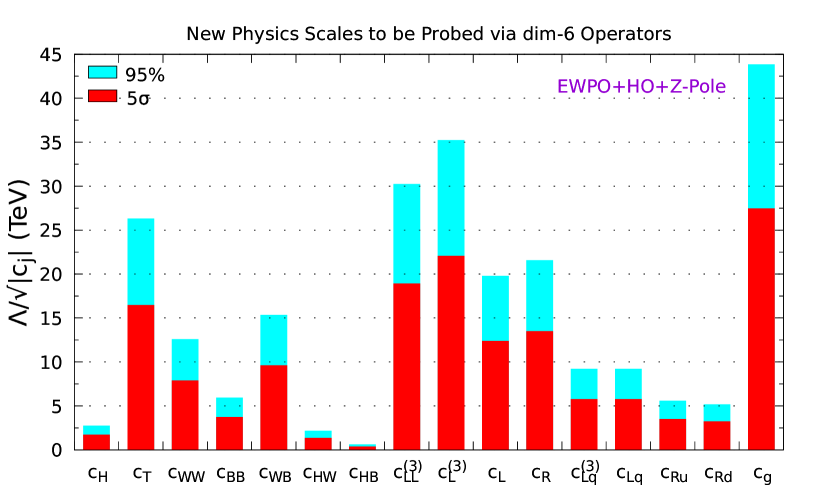
Figure 4: The 95% exclusion (blue) and $5\sigma$ discovery (red) sensitivities to the new physics scales $\,\Lambda/\!\sqrt{|c_{j}|}\,$ by combining the current electroweak precision measurements ($\alpha,\,G_{F},\,M_{Z},\,M_{W}$) PDG14 with the future Higgs observables at the Higgs factory CEPC (Table 2) and $Z$-pole measurements (Table 5) under a projected luminosity of  5 ab^-1 CEPC .

Fig. 4 demonstrates that the $Z$-pole measurements are even more sensitive than the Higgs observables for indirectly constraining the new physics scales of effective dimension-6 operators. This is mainly because of the huge event number that can be produced at the $Z$-pole resonance. We see that running the future $e^{+}e^{-}$ collider at $Z$-pole is beyond the technical purpose of the machine calibration. Our study shows that it is worth of running the collider at $Z$-pole for a longer time. Or, after running the Higgs factory at Higgsstrahlung energy ($240-250$ GeV), it is invaluable to return to the $Z$-pole running for a period and thus ensure the no-lose probe of new physics.

5 Higgs Coupling Precision Tests at CEPC and Probing Dimension-6 Yukawa-type Operators

In this section, we study the CEPC sensitivities to the SM-type Higgs couplings, and then apply these limits to study the probe of Yukawa-type dimension-6 operators (cf. Table 1). In Sec. 5.1, we first apply our analytical linear $\chi^{2}$ fitting method in Appendix B to study the sensitivity probe of the SM-type Higgs couplings at the CEPC. Then, based upon these, we will analyze the CEPC reach of new physics scales associated with the Yukawa-type dimension-6 operators in Sec. 5.2.

5.1 Higgs Coupling Precision Tests at CEPC

For an illustration, we apply the analytical linear $\chi^{2}$ fitting method described in Appendix B to extract the projected precisions of the CEPC Higgs measurements for probing the SM-type Higgs couplings. The Higgs couplings to other SM particles may be defined relative to their SM values by rescaling,  $g_{hii}/g^{\text{sm}}_{hii}\equiv\kappa_{i}\,$, where the possible deviation $\,\kappa_{i}-1\,$ denotes the anomalous Higgs couplings. Such deviations $\,\kappa_{i}-1\,$ can arise from the dimension-6 operators shown in Table 1. The anomalous Higgs couplings $\,\kappa_{i}\neq 1\,$ will modify the Higgs observables in Table 2 and thus receive constraints by the CEPC measurements.

The cross sections of Higgsstrahlung and $WW$ fusion processes are scaled by the Higgs couplings with $Z$ and $W$ gauge bosons as $\,\delta\sigma(Zh)/\sigma(Zh)\simeq 2\delta\kappa_{Z}\,$ and $\,\delta\sigma(\nu\nu h)/\sigma(\nu\nu h)\simeq 2\delta\kappa_{W}$.  On the other hand, each partial decay width of $\,h\rightarrow ii\,$ scales as, $\Gamma_{hii}/\Gamma^{\text{sm}}_{hii}=\kappa^{2}_{i}$.  For the exotic decay channels which are not present in the SM, such as the invisible decays, we can parametrize its contribution as a fraction of the total SM Higgs decay width, $\Gamma_{\mathrm{inv}}/\Gamma^{\mathrm{sm}}_{\textrm{tot}}=\mathrm{Br}(\mathrm{inv})\equiv\delta\kappa_{\mathrm{inv}}$, which is relatively small deviation in principle. Each branching fraction $\,\mathrm{Br}_{i}\,$ is a ratio between the individual decay width and total width, and is thus a function of all scaling factors $\{\kappa_{i}\}$, Since so far the SM fits LHC data quite well and the CEPC measurements can be rather precise, we expect that the relative deviations from the SM are significantly below one, $\,|\kappa_{i}-1|\ll 1$ .  We thus define, $\,\kappa_{i}\equiv 1+\delta\kappa_{i}$,  with $\,|\delta\kappa_{i}|\ll 1$.  Thus, we may expand the branching fractions up to the linear order of $\,\delta\kappa_{i}\,$,

$$\mathrm{Br}^{\mathrm{th}}_{i}\,\simeq\,\mathrm{Br}^{\mathrm{th},0}_{i}\Big{(}1+\sum_{j}A_{ij}\delta\kappa_{j}\Big{)},\qquad~{}~{}\mathrm{Br}^{\mathrm{th}}_{\mathrm{inv}}\,\simeq\,\delta\kappa_{\mathrm{inv}},$$ (54)

where $\,\mathrm{Br}^{\mathrm{th},0}_{i}=\mathrm{Br}^{\mathrm{sm}}_{i}\,$ is the SM prediction, and the coefficient matrix $\,A$  is,

$$A_{ij}=2(\delta_{ij}-\mathrm{Br}^{\mathrm{sm}}_{j}),\qquad A_{i,\mathrm{inv}}=-1,\qquad A_{\mathrm{inv},i}=0,\qquad A_{\mathrm{inv},\mathrm{inv}}=1.$$ (55)

Note that different branching fractions are correlated with coefficient proportional to the corresponding SM values, as shown in (50). For the branching fraction $\mathrm{Br}_{i}$, the contribution due to its own channel is modulated by $\,1-\textrm{Br}^{\text{sm}}_{i}\,$,  while the effect from other channels by the corresponding $\,\mathrm{Br}^{\text{sm}}_{i}$.  Larger branching fraction means the channel has smaller effect on its own, but larger on the others.

Applying our analytical $\chi^{2}$ fitting method (Appendix B) together with the relative uncertainties of Higgs production cross sections and branching fractions from Table 2, we extract the sensitivities of CEPC measurements to the SM Higgs couplings as shown in Table 9 with two different fits in the second and third columns. The first is a 9+1 parameter fit, including 9 parameters for decay branching fractions and 1 for total decay width. All the anomalous Higgs couplings have precisions at $1\%$ level, except that $\,\kappa_{\gamma}\,$ and $\,\kappa_{\mu}\,$ have larger uncertainties. This is because the branching fractions, $\mathrm{Br}(\gamma\gamma)$ and $\mathrm{Br}(\mu\bar{\mu})$, are too small according to the SM predictions hdecay . As shown in Table 2, their values are well below 1%. Since roughly 1 million Higgs particles can be produced at CEPC CEPC , measuring the decays into photon or muon can collect less than $10^{4}$ events. The statistical fluctuation is thus larger than 1%.  A realistic estimate gives  9% and 17%,  respectively, including both statistical and systematic uncertainties. On the contrary, the $ZZh$ Higgs coupling $\,\kappa_{Z}\,$ has a precision much better than $1\%$,  due to the direct measurement of the Higgsstrahlung production cross section $\sigma(Zh)$. This inclusive production rate has larger event rate than any individual decay channel. Without $\sigma(Zh)$, the precision on $\kappa_{Z}$ is also at percentage level. The same thing applies to $\kappa_{W}$,  which can be constrained by the $WW$ fusion production rate $\sigma(\nu\nu h)$, leading to roughly a factor of $\sqrt{2}$  improvement.

Table 9: Projected precisions of measuring Higgs couplings (68% C.L.) at the CEPC (250GeV, 5ab^-1) from our fit, in comparison with the LHC (14TeV, 300fb^-1), HL-LHC (14TeV, 3ab^-1) and ILC (250GeV, 250fb^-1)+(500GeV, 500fb^-1) Peskin .

Precision (%)	CEPC		LHC	HL-LHC	ILC-250	ILC-500
	9+1 fit	8+1 fit
$\kappa_{Z}$	0.249	0.249	8.5	6.3	0.78	0.50
$\kappa_{W}$	1.20	1.20	5.4	3.3	4.6	0.46
$\kappa_{\gamma}$	4.67	4.67	9.0	6.5	18.8	8.6
$\kappa_{g}$	1.42	1.42	6.9	4.8	6.1	2.0
$\kappa_{b}$	1.27	1.27	14.9	8.5	4.7	0.97
$\kappa_{c}$	1.75	1.75	–	–	6.4	2.6
$\kappa_{\tau}$	1.33	1.33	9.5	6.5	5.2	2.0
$\kappa_{\mu}$	8.59	–	–	–	–	–
$\mathrm{Br}(\mathrm{inv})$	0.134	0.134	8.0	4.0	0.54	0.52
$\Gamma_{h}$	2.6	2.6	–	–	–	–

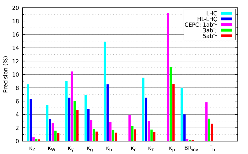
Figure 5: Precisions (68% C.L.) of the CEPC (250 GeV) for measuring the Higgs gauge couplings and Yukawa couplings from our 9+1 parameter fit, with an integrated luminosity of  (1, 3, 5) ab^-1,  respectively. These are compared to the precisions of the LHC (14 TeV, 300 fb^-1) and HL-LHC (14 TeV, 3 ab^-1) Peskin .

For comparison, we further present an 8+1 parameter fit with $\mathrm{Br}(\mu\bar{\mu})$ and $\kappa_{\mu}$ removed in the third column of Table 9. We note that the precision of measuring other anomalous couplings are not affected at all. This is because the branching fraction of this channel is very small in the first place. As explained below Eq. (55), the correlation is proportional to the corresponding SM prediction $\,\mathrm{Br}^{\text{sm}}_{j}$.  Hence, it is rather weakly correlated with other channels. We present the result of these two fits in Fig. 5.

Besides the precision limits on Higgs couplings at the CEPC (250 GeV, 5 ab^-1), we also show the bounds on Higgs couplings from the LHC (14 TeV, 300 fb^-1) and the HL-LHC (14 TeV, 3 ab^-1) Peskin , in Table 9, for comparison. It is clear that the CEPC (250 GeV, 5 ab^-1) can significantly improve the precision of Higgs coupling measurements. In addition, many decay channels cannot be probed at the LHC. For instance, the LHC has no sensitivity to the $\,hc\bar{c}\,$ coupling Peskin , as well as $h\mu\bar{\mu}$ coupling. But, they can be measured at the CEPC instead. The total decay width of the SM Higgs with $125\,$GeV mass is about $4$ MeV,  which is far below the LHC sensitivity. It is hard to make a direct measurement at the LHC without model assumptions. In Table 9, we also show the projected limits of the ILC (250 GeV, 250 fb^-1) and ILC (500 GeV, 500 fb^-1) for comparison Peskin . It shows that CEPC (250GeV, 5ab^-1) can have better sensitivities than the ILC (500GeV, 500fb^-1), except for the $hWW$ and $hb\bar{b}$ couplings.

5.2 Probing Dimension-6 Yukawa-type Operators at CEPC

The last column of Table 1 also presents three Yukawa-type dimension-6 operators $\,\mathcal{O}_{y}^{f}=(\mathcal{O}_{y}^{u},\,\mathcal{O}_{y}^{d},\,\mathcal{O}_{y}^{\ell})$.  These operators will modify the SM Yukawa coupling by a rescaling factor,

$$y_{f}^{\text{sm}}~{}~{}\longrightarrow~{}~{}y_{f}\,=\,y_{f}^{\text{sm}}+\frac{\,3c_{f}v^{2}\,}{2\Lambda^{2}}\,,$$ (56)

and correct the SM fermion mass,

$$m_{f}^{\text{sm}}=\frac{y_{f}^{\textrm{sm}}v}{\sqrt{2}}\,~{}~{}\longrightarrow~{}~{}m_{f}\,=\,\frac{v}{\sqrt{2}\,}\!\left(\!y_{f}^{\text{sm}}+\frac{\,c_{f}v^{2}\,}{\,2\Lambda^{2}\,}\!\right)\!,$$ (57)

where $\,m_{f}\,$ is the full fermion mass including contributions of dimension-6 operators. Thus, using (57), we can reexpress $\,y_{f}^{\text{sm}}\,$ as

$$y_{f}^{\textrm{sm}}\,=\,\frac{\,\sqrt{2}m_{f}\,}{v}-\frac{\,c_{f}v^{2}\,}{\,2\Lambda^{2}\,}\,=\,y_{f}^{\textrm{sm},0}-\frac{\,c_{f}v^{2}\,}{\,2\Lambda^{2}\,},$$ (58)

where $\,y_{f}^{\textrm{sm},0}\equiv\sqrt{2}m_{f}/v\,$.  From Eqs. (56) and (58), we compute the coupling ratios up to $\mathcal{O}(\Lambda^{-2})$,

$$\kappa_{f} = \frac{\,y_{f}\,}{\,y_{f}^{\textrm{sm}}\,}\,\simeq\,1+\frac{3c_{f}v^{3}}{\,2\sqrt{2}\,m_{f}\Lambda^{2}\,}\,,$$ (59a)

$$y_{f} = y_{f}^{\textrm{sm},0}\left(y_{f}/y_{f}^{\textrm{sm},0}\right)\,=\,y_{f}^{\textrm{sm},0}\tilde{\kappa}_{f}\,,$$ (59b)

$$\tilde{\kappa}_{f} \equiv \frac{y_{f}}{\,y_{f}^{\textrm{sm},0}\,}\,=\,\frac{y_{f}^{\textrm{sm}}}{\,y_{f}^{\textrm{sm},0}\,}\kappa_{f}\,\simeq\,1+\frac{c_{f}v^{3}}{\,\sqrt{2}\,m_{f}\Lambda^{2}\,}\,.$$ (59c)

We note that it is the effective coupling $\,y_{f}\,$ that actually enters the physical observables, and the $\chi^{2}$ fit we made in Sec. 5.1 (Table 9) is just a fit of the sensitivity reach on the coupling ratio $\,\tilde{\kappa}_{f}\equiv{y_{f}}/{\,y_{f}^{\textrm{sm},0}\,}\equiv 1+\Delta\tilde{\kappa}_{f}\,$,  for the case of Higgs Yukawa couplings, where $\,\Delta\tilde{\kappa}=\tilde{\kappa}_{f}-1\,$ is given by Eq. (59c) for the contribution of dimension-6 operator $\,\mathcal{O}_{y}^{f}\,$.  This means that each $\,\kappa_{f}\,$ in Table 9 should be replaced by the current notation $\,\tilde{\kappa}_{f}\,$ as we exactly defined in Eq. (59c).

Table 10: Sensitivity reaches (95% C.L.) of the new physics scales of Yukawa-type dimension-6 operators at the CEPC (250GeV, 5ab^-1), in comparison with the LHC (14TeV, 300fb^-1), HL-LHC (14TeV, 3ab^-1), and ILC (250GeV, 250fb^-1)+(500GeV, 500fb^-1).

$\Lambda/\!\sqrt{|c_{j}|}(\mbox{TeV})$	CEPC		LHC	HL-LHC	ILC-250	ILC-500
	9+1 fit	8+1 fit
$b$ quark	13.2	13.2	3.87	5.12	6.89	15.2
$c$ quark	24.4	24.4	–	–	12.8	20.0
$\tau$ lepton	15.4	15.4	5.74	6.95	7.76	12.5
$\mu$ lepton	25.1	–	–	–	–	–

Thus, for each given fitted experimental sensitivity $\,\Delta\tilde{\kappa}_{f}\,$ (Table 9) and using Eq. (59c), we can derive the following lower bound on the Yukawa-type new physics scale,

$$\frac{\Lambda}{\sqrt{|c_{f}|\,}\,}~{}\geqslant~{}\sqrt{\frac{v^{3}}{\,\sqrt{2}\,m_{f}\Delta\tilde{\kappa}_{f}\,}\,}\,.$$ (60)

In Eq. (60), the Yukawa coupling precision $\,\Delta\tilde{\kappa}_{f}\,$ will be measured at the CEPC with a typical renormalization scale $\,\mu=M_{h}\,$.  So we will input the fermion mass $\,m_{f}\,$ as the running mass defined at $\,\mu=M_{h}\,$.  With these, we present the CEPC potential reaches (95% C.L.) in Fig. 6 and Table 10, and compare them with the corresponding limits estimated for the LHC (14TeV, 300fb^-1), HL-LHC (14TeV, 3ab^-1), and ILC (250GeV, 250fb^-1)+(500GeV, 500fb^-1) Peskin . We see that depending on the experimental precision and the involved fermion mass, the CEPC probe of the Yukawa-type new physics scales can reach $\,13-25\,\mbox{TeV}$ range with a $5\,\mbox{ab}^{-1}$ integrated luminosity. These sensitivities are much higher than that of the LHC Run-2 and the HL-LHC.

From Fig. 6 and Table 10, it is interesting to see that the probe of the new physics scales with operators $\,\mathcal{O}_{y}^{\mu}\,$ and $\,\mathcal{O}_{y}^{c}\,$ are significantly better than other Yukawa-type operators such as $\,(\mathcal{O}_{y}^{b},\,\mathcal{O}_{y}^{\tau})\,$.  This is because the lower bound (60) is proportional to $(m_{f}\Delta\tilde{\kappa}_{f})^{-1/2}$,  which depends on both the coupling precision $\,\Delta\tilde{\kappa}_{f}\,$ and the fermion mass $\,m_{f}\,$.  Here we have used the running masses mass-run PDG2014 , $(m_{b},\,m_{c},\,m_{\tau},\,m_{\mu})\simeq(2.41,\,0.515,\,1.713,\,0.0996)$GeV, at the scale $\,\mu=M_{h}\,$.  As shown in Table 9 and Fig. 5, among the sensitivities to $(\tilde{\kappa}_{b},\,\tilde{\kappa}_{c},\,\tilde{\kappa}_{\tau},\,\tilde{\kappa}_{\mu})$,  CEPC can measure $\,\tilde{\kappa}_{b}\,$ most precisely (down to a relative precision $\Delta\tilde{\kappa}_{b}=1.27\%$), and probe $\,\tilde{\kappa}_{\mu}\,$ least precisely (down to $\Delta\tilde{\kappa}_{\mu}=8.59\%$), which differ by a factor 6.76.  But, their running masses differ by a much larger ratio $\,m_{b}/m_{\mu}\simeq\,24.2$ .  This means that the fermion mass ratio has larger effect than the ratio of their coupling sensitivities. Hence, we find that the reach of new physics scale with $\,\mathcal{O}_{y}^{\mu}\,$ is higher than that with $\,\mathcal{O}_{y}^{b}\,$ by a factor of $\,\sqrt{24.2/6.76}\simeq 1.9$ .  This explains our findings shown in Table 10  and Fig. 6 . Similarly, for the other two operators $\,(\mathcal{O}_{y}^{c},\,\mathcal{O}_{y}^{\tau})\,$ with fermions  $(c,\,\tau)$,  we can deduce that the corresponding reaches of new physics scales are enhanced relative to that of $\,\mathcal{O}_{y}^{b}\,$ by a factor about $(1.8,\,1.2)$.

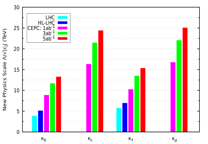
Figure 6: Sensitivity reaches (95% C.L.) of the new physics scales $\,\Lambda/\!\sqrt{|c_{j}|}$  of Yukawa-type dimension-6 operators by the precision Higgs coupling measurements at the Higgs factory CEPC (250GeV), in comparison with LHC (14TeV, 300fb^-1) and the HL-LHC (14TeV, 3ab${}^{-1})$.

6 Conclusions

The LHC Higgs discovery in 2012 has led particle physics to a turning point, at which the precision Higgs measurements have become an important task for seeking clues to the new physics discovery. A future Higgs factory (like the proposed $e^{+}e^{-}$ colliders CEPC, FCC-ee, and ILC) can provide such precision Higgs measurements.

In this work, we studied the new physics scales that a future Higgs factory can probe via general dimension-6 operators involving the observed Higgs boson (Table 1). Our analysis utilizes the existing electroweak precision observables (EWPO), as well as the Higgs observables and precision measurements at the future $e^{+}e^{-}$ Higgs factory (taking the CEPC as an illustration). The conventional scheme-dependent analysis usually fixes the three electroweak parameters ($g$, $g^{\prime}$, $v$) with three high precision electroweak observables ($\alpha,G_{F},M_{Z}$) in the $Z$-scheme or ($\alpha,M_{W},M_{Z}$) in the $W$-scheme, while ignoring their experimental uncertainties. In contrast, we developed a scheme-independent approach to incorporate full experimental information (including both central values and uncertainties) of the EWPO in Section 2. With this approach, the electroweak parameters and the new physics scales of dimension-6 operators can be fitted simultaneously by the same $\chi^{2}$ function.

The advantage of our scheme-independent approach is made clear when the precisions of $Z$ and $W$ mass measurements become comparable at the Higgs factory (cf. Table 6). Since new physics deviations from the SM are fairly small, as already constrained by the LHC data, the analytical expansion up to their linear order holds well (Section 3). Accordingly, we performed the analytic linear $\chi^{2}$ fit in Appendix B, which is physically intuitive, numerically fast, and can be straightforwardly generalized to include any number of observables and fitting parameters under consideration. In Section 4, we demonstrated that including the existing EWPO together with future Higgs measurements can probe the new physics scales up to 10 TeV (and to 44 TeV for the gluon-involved operator $\mathcal{O}_{g}$) at 95% C.L., as shown in Fig. 3 and Table 3. We found that including the CEPC precision measurements can further lift the reach up to 35 TeV (Fig. 4 and Table 8). In addition, the CEPC precision tests of Higgs couplings can probe the new physics scales with Yukawa-type operators up to $(13-25)$ TeV, (Fig. 6 and Table 10). We note that these indirect new physics reaches do cover the energy range to be probed by the future hadron colliders of $pp(50-100)$ TeV CEPC ; FCC-ee running in the same circular tunnel. Hence, the precision probe at the Higgs factory can provide an important guideline for the future new physics discoveries at the SPPC or FCC-hh. Our study demonstrates that the Higgs factory can probe the new physics of the Higgs sector much more sensitively than what the LHC would achieve LHCeff .

The $Z$-pole running of the $e^{+}e^{-}$ collider is required by the machine calibration at its initial stage. In Section 4.6, we further demonstrated that during the CEPC early phase, the $Z$-pole measurements can provide even stronger indirect probe of the new physics scales than the Higgs observables alone as measured at the Higgs factory ($250$GeV). This motivates a longer $Z$-pole running to ensure the no-lose probe of new physics deviations from the SM, complementary to the Higgs factory via the $Zh$ production.

Appendix A Kinetic Mixing of Gauge Bosons

The dimension-6 operators can make nontrivial corrections to both the mass matrices and the kinetic terms of gauge bosons. The situation is much simpler for charged weak bosons $W^{\pm}$ which have only one mass eigenstate and thus no extra mixing in the effective theory of the SM with dimension-6 operators. On the other hand, the situation for neutral gauge bosons are more involved since mixing between the photon $A$ and the $Z$ boson can arise from either loop corrections or new physics beyond the SM. Both kinetic mixing and mass diagonalization may appear. It is necessary to first transform their kinetic terms into the canonical forms and mass matrix into the diagonal form before deriving Feynman rules and computing physical processes. Here, we provide a general formalism within this effective theory, and describe how to deal with the corrections from dimension-6 operators up to the linear order.

A.1 Charged Gauge Bosons

For charged gauge boson, there is no mixing in either kinetic or mass term,

$${\bf D}(q^{2})\,=~{}\frac{1}{\,q^{2}K-\left[(M^{(0)}_{W})^{2}-\delta M^{2}_{W}\right]\,}\,,$$ (61)

where $\,K\equiv 1+\delta K=Z_{W}^{-2}\,$ with $\,Z_{W}\,$ given by Eq.(9). Thus, we have

$$\delta K\,\simeq\,-2\delta Z_{W}\,=\,-\frac{\,2v^{2}}{\,\Lambda^{2}\,}g^{2}c_{WW}\,.$$ (62)

The propagator (61) reduces to its canonical form, ${\bf D}(q^{2})=\frac{1}{\,q^{2}-M^{2}_{W}\,}$, when the $W$ boson field and its mass are renormalized as

$$W\rightarrow\frac{W}{\sqrt{K\,}\,}\,,\qquad M^{2}_{W}=\left(\!M^{(0)}_{W}\right)^{\!2}\!\left(\!1+\frac{\delta M^{2}_{W}}{M^{2}_{W}}-\delta K\!\right)\!.$$ (63)

Here we have omitted the small difference between $M_{W}$ and $M^{(0)}_{W}$ in the denominator of the second term, which is of the higher order.

A.2 Neutral Gauge Bosons

For neutral gauge bosons, both $A$ and $Z$ are involved. The kinetic mixing and mass terms are hence $2\!\times\!2$ matrices. Nontrivial mixing effects can appear in both parts. We first generally parametrize the correlated propagator as

$${\bf D}(q^{2})\,=\,\frac{1}{\,q^{2}\mathbb{K}-\mathbb{M}^{2}\,}\,,$$ (64)

where both kinetic coefficient matrix $\mathbb{K}$ and the mass matrix $\mathbb{M}$ need to be diagonalized, $S\mathbb{K}S^{-1}\equiv\mathbb{T}$ and $R\mathbb{M}^{2}R^{-1}\equiv\mathbb{D}^{2}$, with $\,\mathbb{T}\,$ and  $\mathbb{D}$  denoting the diagonal kinetic matrix and diagonal mass matrix, respectively. Then, we can first diagonalize the kinetic term as

$${\bf D}(q^{2})\,=\,\frac{1}{\,q^{2}S^{-1}\mathbb{T}S-\mathbb{M}^{2}\,}\,=\,S^{-1}\mathbb{T}^{-\frac{1}{2}}\frac{1}{\,q^{2}\mathbb{I}-\mathbb{T}^{-\frac{1}{2}}S\mathbb{M}^{2}S^{-1}\mathbb{T}^{-\frac{1}{2}}\,}\mathbb{T}^{-\frac{1}{2}}S\,,~{}~{}~{}~{}~{}$$ (65)

by folding kinetic mixing to the mass matrix, $\,\widetilde{\mathbb{M}}^{2}\equiv\mathbb{T}^{-\frac{1}{2}}S\mathbb{M}^{2}S^{-1}\mathbb{T}^{-\frac{1}{2}}$. The modified mass matrix can be diagonalized by $\,\widetilde{\mathbb{M}}^{2}\,=\,\widetilde{R}^{-1}\widetilde{\mathbb{D}}^{2}\widetilde{R}\,$.  Then, the propagator can be reduced to the fully diagonalized form,

$${\bf D}(q^{2})\,=\,S^{-1}\mathbb{T}^{-\frac{1}{2}}\widetilde{R}^{-1}\frac{1}{\,q^{2}\mathbb{I}-\widetilde{\mathbb{D}}^{2}\,}\widetilde{R}\mathbb{T}^{-\frac{1}{2}}S\,\equiv\,\widetilde{S}^{T}\frac{1}{\,q^{2}\mathbb{I}-\widetilde{\mathbb{D}}^{2}\,}\widetilde{S}\,.$$ (66)

For the current effective theory, the original mass matrix $\,\mathbb{M}^{2}=\mbox{diag}\{0,M^{2}_{Z}\}$  of neutral gauge bosons is diagonalized in the $A$-$Z$ space. It should be noted that $\,M^{2}_{Z}\equiv(M^{(0)}_{Z})^{2}+\delta M^{2}_{Z}$  is already the value after including the dimension-6 operator contributions. It remains diagonalized because of the unbroken $U(1)_{\text{em}}$ gauge symmetry requires, $\,\Pi_{AA}(0)=\Pi_{AZ}(0)=0$,  when writing down the effective operators. On the other hand, for generality, kinetic mixing can be parametrized as, $\mathbb{K}\equiv\mathbb{I}+\delta K$,  where $\delta K$ is a $2\times 2$ symmetric matrix whose explicit form will be given at the end of this section. A general feature is that its matrix elements  $(\delta K_{11},\delta K_{12},\delta K_{22})$  belong to the linear order in terms of dimension-6 operator coefficients. This leads to a sizable mixing of order $\mathcal{O}(1)$,

$$S\,\equiv\left\lgroup\begin{matrix}\cos\theta&\sin\theta\\ -\sin\theta~{}\,&\cos\theta\end{matrix}\right\rgroup\!\!,\quad\quad\tan 2\theta=\frac{2\delta K_{12}}{\,\delta K_{11}-\delta K_{22}\,},$$ (67)

under which the kinetic term becomes diagonal. But, the deviations from canonical form are still of the linear order, $\,\mathbb{T}\equiv\mbox{diag}\{1+\delta K_{1},1+\delta K_{2}\}$,  which is a diagonal matrix. Then, the modified mass matrix $\,\widetilde{\mathbb{M}}^{2}$  of neutral gauge bosons becomes,

$$\widetilde{\mathbb{M}}^{2}\,\equiv\,\mathbb{T}^{-\frac{1}{2}}S\mathbb{M}^{2}S^{-1}\mathbb{T}^{-\frac{1}{2}}\,=\,M^{2}_{Z}\!\left\lgroup\begin{matrix}\frac{\sin^{2}\theta}{1+\delta K_{1}}&\frac{\cos\theta\sin\theta}{\sqrt{1+\delta K_{1}}\sqrt{1+\delta K_{2}}}\\[5.69054pt] \frac{\cos\theta\sin\theta}{\sqrt{1+\delta K_{1}}\sqrt{1+\delta K_{2}}}&\frac{\cos^{2}\theta}{1+\delta K_{2}}\end{matrix}\right\rgroup\!.~{}~{}~{}~{}~{}$$ (68)

Since the rank of $\widetilde{\mathbb{M}}^{2}$ equals 1, it contains a massless eigenstate as the photon. This property is a consequence of the unbroken $U(1)_{\text{em}}$ gauge symmetry. In addition, the $Z$ boson mass is modified as

$$\widetilde{M}^{2}_{Z}\,\simeq\,M^{2}_{Z}\left(1\!-\sin^{2}\!\theta\delta\,K_{1}\!-\cos^{2}\!\theta\delta\,K_{2}\right)\,=\,\left[M^{(0)}_{Z}\right]^{2}\!\!\left(\!1+\frac{\delta M^{2}_{Z}}{M^{2}_{Z}}-\delta K_{22}\!\right)\!.$$ (69)

For convenience, we have denoted the zeroth-order of $Z$ boson mass as $M^{(0)}_{Z}$ and the correction as $\,\delta M^{2}_{Z}\,$ which is independent of the correction from kinetic mixing. The modified mixing matrix $\,\widetilde{R}\,$ is

$$\widetilde{R}\,=\left\lgroup\begin{matrix}\cot\!\theta\,\sqrt{\frac{1+\delta K_{1}}{1+\delta K_{2}+\cot^{2}\theta(1+\delta K_{1})}}~{}~{}&-\sqrt{\frac{1+\delta K_{2}}{1+\delta K_{2}+\cot^{2}\theta(1+\delta K_{1})}}\\[11.38109pt] \tan\!\theta\,\sqrt{\frac{1+\delta K_{2}}{1+\delta K_{1}+\tan^{2}\theta(1+\delta K_{2})}}~{}~{}&\sqrt{\frac{1+\delta K_{1}}{1+\delta K_{1}+\tan^{2}\theta(1+\delta K_{2})}}\end{matrix}\,\right\rgroup\!\!.$$ (70)

Altogether, we can derive the full current rotation $\,\widetilde{S}$ ,

$$\widetilde{S}\,\equiv\,\widetilde{R}\mathbb{T}^{-\frac{1}{2}}S\,=\,\mathbb{I}-\frac{1}{2}\!\left\lgroup\begin{matrix}\delta K_{11}\,&\,0\\[2.84526pt] 2\delta K_{12}\,&\,\delta K_{22}\end{matrix}\right\rgroup\!.$$ (71)

The mixing matrix $\,\widetilde{S}\,$ rotates $A$ and $Z$ as well as their corresponding currents,

$$\widetilde{J}\,\equiv\,\widetilde{S}J\,=\left\lgroup\begin{matrix}\left(1\!-\!\frac{1}{2}\delta K_{11}\right)\!J_{A}&0\\[4.2679pt] 0&~{}-\delta K_{12}J_{A}\!+\!\left(1\!-\!\frac{1}{2}\delta K_{22}\right)\!J_{Z}\end{matrix}\right\rgroup\!.$$ (72)

Note that this result still has linear dependence on the dimension-6 operator coefficients. The corrections to the kinetic term can lead to not only the field redefinitions of $A$ and $Z$, but also the mixing between them.

For the effective operators under consideration, the $\,\delta K\,$ matrix elements are

$$\delta K_{11} = \frac{-2v^{2}}{\Lambda^{2}}\left[s^{2}_{w}g^{2}c_{WW}\!-\!c_{w}s_{w}gg^{\prime}c_{WB}\!+\!c^{2}_{w}g^{\prime 2}c_{BB}\right]\!,$$ (73a)

$$\delta K_{12} = \frac{-2v^{2}}{\Lambda^{2}}\left[c_{w}s_{w}g^{2}c_{WW}\!-\!\frac{1}{2}(c^{2}_{w}\!-\!s^{2}_{w})gg^{\prime}c_{WB}\!-\!c_{w}s_{w}g^{\prime 2}c_{BB}\right]\!,$$ (73b)

$$\delta K_{22} = \frac{-2v^{2}}{\Lambda^{2}}\left[c^{2}_{w}g^{2}c_{WW}\!+\!c_{w}s_{w}gg^{\prime}c_{WB}\!+\!s^{2}_{w}g^{\prime 2}c_{BB}\right]\!,$$ (73c)

which involve only three operators, $\mathcal{O}_{WW}$, $\mathcal{O}_{BB}$, and $\mathcal{O}_{WB}$ .

Appendix B Analytic Linear $\chi^{2}$ Fit

To make our analysis fully transparent, in this Appendix we present the $\chi^{2}$ fitting method used for the current study. With a set of observables $\mathcal{O}_{j}$ to constrain model parameters, we need to minimize the $\chi^{2}$ function,

$$\chi^{2}~{}=\,\sum_{j}\left(\frac{\mathcal{O}^{\mathrm{th}}_{j}-\mathcal{O}^{\mathrm{exp}}_{j}}{\Delta\mathcal{O}_{j}}\right)^{\!2},$$ (74)

which is a summation of individual constraints. In the above, we use $\mathcal{O}^{\text{th}}_{j}$ to denote the theoretical prediction, $\mathcal{O}^{\mathrm{exp}}_{j}$ the experimental measurement, and $\,\Delta\mathcal{O}_{j}\,$ the associated uncertainty. The theoretical prediction is a function of model parameters. Here, we will just use the $\,\kappa_{j}\,$ rescaling of the Higgs coupling with the SM particles to fit experimental data (as to be elaborated in Appendix 5), for an illustration. The deviation from the SM is then parametrized as $\,\delta\kappa_{j}\equiv\kappa_{j}-1\,$,  which are small numbers. When expanded to the linear term of $\,\delta\kappa_{j}$,  the $\chi^{2}$ function can be expressed as a quadratic function with matrix manipulations,

$$\chi^{2}\,=\,(\mathcal{O}^{\text{th,0}}\!+A\delta\kappa-\mathcal{O}^{\text{exp}})^{T}\,\overline{\Sigma}^{-1}(\mathcal{O}^{\text{th,0}}\!+A\delta\kappa-\mathcal{O}^{\text{exp}})\,.$$ (75)

Note that, in matrix notations, the observable $\,\mathcal{O}\,$ has dimension $\,m\!\times\!1$,  the deviation $\delta\kappa$ has dimension $\,n\!\times\!1$,  coefficient matrix $A$ has dimension $\,m\!\times\!n$,  and error matrix $\,\overline{\Sigma}\,$ dimension $\,m\!\times\!m$,  where $m$ and $n$ are the number of observables and model/fitting parameters, respectively. The error matrix $\,\overline{\Sigma}^{-1}\,$ of independent measurements is diagonal,

$$\overline{\Sigma}^{-1}=\,\mbox{diag}\left\{\frac{1}{(\Delta\mathcal{O}_{1})^{2}},\,\frac{1}{(\Delta\mathcal{O}_{2})^{2}},\,\cdots\!,\,\frac{1}{(\Delta\mathcal{O}_{n})^{2}}\right\},$$ (76)

according to the definition in (74). This corresponds to uncorrelated/independent measurements. Nevertheless, this assumption is not necessary. For correlated/dependent measurements, the error matrix $\,\overline{\Sigma}^{-1}$  in the observable basis is in general a symmetric matrix, $\overline{\Sigma}_{ij}\equiv\sigma_{i}\rho_{ij}\sigma_{j}$,  where $\,\rho\,$ is the so-called correlation matrix.

The $\chi^{2}$ function reaches its minimum under the condition, $\,\partial\chi^{2}/\partial\delta\kappa_{j}=0$ .  From this, we can solve the best fit values of $\delta\kappa$,

$$\delta\kappa_{\text{best}}\,=~{}(A^{T}\,\overline{\Sigma}^{-1}\!A)^{-1}A^{T}\,\overline{\Sigma}^{-1}\!\left(\mathcal{O}^{\text{exp}}\!-\mathcal{O}^{\text{th,0}}\right).$$ (77)

For convenience, let us rewrite the $\chi^{2}$ function in the fitting parameter basis,

$$\chi^{2}\,=~{}\chi^{2}_{\text{min}}+(\delta\kappa-\delta\kappa_{\text{best}})^{T}\Sigma^{-1}(\delta\kappa-\delta\kappa_{\text{best}}),$$ (78)

where the error matrix $\,\Sigma\equiv A^{T}\,\overline{\Sigma}^{-1}A\,$ can be obtained from $\,\overline{\Sigma}\,$ through matrix manipulation, and has dimension $\,n\times n$.  Note that the error matrix $\,\Sigma^{-1}\,$ is also symmetric. The $\chi^{2}_{\text{min}}$ can also be expressed analytically, $\,\chi^{2}_{\text{min}}=~{}(\mathcal{O}^{\text{exp}}\!-\mathcal{O}^{\text{th,0}})^{T}B^{T}\overline{\Sigma}^{-1}B(\mathcal{O}^{\text{exp}}\!-\mathcal{O}^{\text{th,0}})$,  where $\,B\equiv\mathbb{I}-A(A^{T}\,\overline{\Sigma}^{-1}A)^{-1}A^{T}\,\overline{\Sigma}^{-1}$.  If the theoretical prediction is consistent with experimental measurement, $\,\mathcal{O}^{\mathrm{th},0}_{j}\!=\mathcal{O}^{\mathrm{exp}}_{j}$,  the $\chi^{2}$ function reaches the minimum at the SM values, $\,\delta\kappa_{j}=0$,  which is the best value. This formalism of analytic $\chi^{2}$ function can even be used to estimate the statistical fluctuation in $\chi^{2}_{\min}$ Ge:2012wj .

In general, different fitting parameters are correlated with each other through the coefficient matrix $A$ and hence can affect each other. To obtain the precision of a specific fitting parameter, we need to marginalize over the others. This can be done as a series of iterative reductions from higher-dimensional $\chi^{2}$ function to lower one, each time reducing the number of fitting parameters by $1$. During this process, the $\chi^{2}$ function can still be expressed with the quadratic form (78) in the fitting parameter basis while the n-dimensional error matrix $\,\Sigma\,$ can be reduced to $(n-1)$-dimensional $\,\widetilde{\Sigma}\,$ by integrating out one degree of freedom, say the $k$-th branching fraction,

$$\widetilde{\Sigma}^{-1}_{ij}~{}=~{}\Sigma^{-1}_{ij}-\frac{\,\Sigma^{-1}_{ik}\Sigma^{-1}_{jk}\,}{\Sigma^{-1}_{kk}}.$$ (79)

Note that there is no summation over $k$. This reduction formula is just a reflection of integrating out the $k$-th degree of freedom from the probability distribution $\,\mathbb{P}(\delta\kappa_{j})\equiv\mathrm{exp}(-\chi^{2}/2)$,

$$\mathbb{P}(\delta\kappa_{1}\cdots\delta\hat{\kappa}_{k}\cdots\delta\kappa_{n})~{}=\,\int^{+\infty}_{-\infty}\mathbb{P}(\delta\kappa_{1}\cdots\delta\kappa_{k}\cdots\delta\kappa_{n})\,\text{d}\delta\kappa_{k}\,.$$ (80)

The hat means that the corresponding variable has been integrated out. With quadratic $\chi^{2}$, this is an integration of Gaussian distribution that can be done analytically to produce (79). The same procedure should be carried out until there is only one degree of freedom left, say, the $\ell$-th anomalous coupling. The only element of the 1-dimensional error matrix is then its uncertainty, $\,\Delta(\delta\kappa_{\ell})\equiv\sqrt{\widetilde{\Sigma}_{\ell\ell}}$ .  To deduce the precision of all fitting parameters, we need to run over all possible values of $\,\ell\,$ and make the reduction for each case. This analytic $\chi^{2}$ fitting technique, along with other extensions, will be delivered in a general purpose package BSMfitter BSMfitter .

References

- (1) G. Aad et al. [ATLAS Collaboration], Phys. Lett. B 716 (2012) 1 [arXiv:1207.7214 [hep-ex]]; S. Chatrchyan et al. [CMS Collaboration], Phys. Lett. B 716 (2012) 30 [arXiv:1207.7235 [hep-ex]].
- (2) F. Englert and R. Brout, Phys. Rev. Lett. 13 (1964) 321. P. W. Higgs, Phys. Lett. 12 (1964) 132; Phys. Rev. Lett. 13 (1964) 508; G. S. Guralnik, C. R. Hagen, and T. Kibble, Phys. Rev. Lett. 13 (1965) 585; T. Kibble, Phys. Rev. 155 (1967) 1554.
- (3) J. Ellis, M. K. Gaillard and D. V. Nanopoulos, “An Updated Historical Profile of the Higgs Boson”, arXiv:1504.07217 [hep-ph]; and references therein.
- (4) For recent review, e.g., John Ellis, “Summary and Outlook: 2015 Lepton-Photon Symposium”, arXiv:1509.07336, in the proceedings of International Symposium on Lepton Photon Interactions at High Energies, August 17-22, 2015, Slovenia.
- (5) Nima Arkani-Hamed, “Vision for the Future”, presented at the Workshop on Physics at the CEPC, August 10-12, 2015, IHEP, Beijing, http://indico.ihep.ac.cn/event/4937.
- (6) Michael E. Peskin, “Estimation of LHC and ILC Capabilities for Precision Higgs Boson Coupling Measurements”, in the proceedings of Snowmass 2013, [arXiv:1312.4974 [hep-ph]].
- (7) D. A. Dicus and H. J. He, Phys. Rev. Lett. 94 (2005) 221802 [hep-ph/0502178]; Phys. Rev. D 71 (2005) 093009 [hep-ph/0409131].
-
(8)
K. G. Wilson, Phys. Rev. D 3 (1971) 1818;
L. Susskind, Phys. Rev. D 20 (1979) 2619.
For a recent review, G. Altarelli, Frascati Phys. Ser. 58 (2014) 102 [arXiv:1407.2122]. -
(9)
F. L. Bezrukov and M. Shaposhnikov,
Phys. Lett. B 659 (2008) 703 [arXiv:0710.3755];
F. Bezrukov, Class. Quant. Grav. 30 (2013) 214001 [arXiv:1307.0708]; and references therein. - (10) E.g., D. Bauer et al., Phys. Dark Univ. 7-8 (2015) 16 [arXiv:1305.1605]; S. Arrenberg et al., arXiv:1310.8621, Snowmass 2013 CF4 Working Group Report; J. Ren and H. J. He, JCAP 1503 (2015) 052 [arXiv:1410.6436]; Y. Bai, V. Barger, L. L. Everett, G. Shaughnessy, Phys. Rev. D 88 (2013) 015008 [arXiv:1212.5604]; and references therein.
- (11) E.g., J. R. Espinosa, G. F. Giudice, and A. Riotto, JCAP 0805 (2008) 002 [arXiv:0710.2484]; J. Ellis, J. R. Espinosa, G. F. Giudice, A. Hoecker and A. Riotto, Phys. Lett. B 679 (2009) 369 [arXiv:0906.0954 [hep-ph]]; A. Kobakhidze and A. Spencer-Smith, Phys. Lett. B 722 (2013) 130 [arXiv:1301.2846]; K. Enqvist, T. Meriniemi and S. Nurmi, JCAP 1310 (2013) 057 [arXiv:1306.4511]; M. Fairbairn and R. Hogan, Phys. Rev. Lett. 112 (2014) 201801 [arXiv:1403.6786]; K. Enqvist, T. Meriniemi and S. Nurmi, JCAP 1407 (2014) 025 [arXiv:1404.3699]; M. Herranen, T. Markkanen, S. Nurmi and A. Rajantie, Phys. Rev. Lett. 113 (2014) 211102 [arXiv:1407.3141]; K. Kamada, Phys. Lett. B 742 (2015) 126 [arXiv:1409.5078]; A. Spencer-Smith, arXiv:1405.1975; A. Shkerin and S. Sibiryakov, Phys. Lett. B 746 (2015) 257 [arXiv:1503.02586]; A. Hook, J. Kearney, B. Shakya, and K. M. Zurek, JHEP 1501 (2015) 061 [arXiv:1404.5953]; J. Kearney, H. Yoo, and K. M. Zurek, Phys. Rev. D 91 (2015) 123537 [arXiv:1503.05193]; J. R. Espinosa, G. F. Giudice, E. Morgante, A. Riotto, L. Senatore, and A. Strumia, N. Tetradis, JHEP 1509 (2015) 174 [arXiv:1505.04825]; and references therein.
- (12) E.g., J. Ellis and D. Ross, Phys. Lett. B 506 (2001) 331 [arXiv:hep-ph/0012067]; H. J. He and Z. Z. Xianyu, JCAP 1410 (2014) 019 [arXiv:1405.7331]; Z. Z. Xianyu and H. J. He, JCAP 1410 (2014) 083 [arXiv:1407.6993]; J. Ellis, H. J. He, Z. Z. Xianyu, Phys. Rev. D 91 (2015) 021302 [arXiv:1411.5537]; and JCAP 1608 (2016) 068 [arXiv:1606.02202]; S. F. Ge, H. J. He, J. Ren, Z. Z. Xianyu, Phys. Lett. B 757 (2016) 480 [arXiv:1602.01801]; and references therein.
- (13) CEPC Collaboration, http://cepc.ihep.ac.cn, “CEPC-SPPC preliminary conceptual design report”; and M. Ruan, [arXiv:1411.5606 [hep-ex]], “Higgs measurement at circular colliders”, presentation at 37th International Conference on High Energy Physics (ICHEP-2014), July 2-9, 2014, Valencia, Spain; and M. Ruan, “Higgs Physics at CEPC”, talk at KITPC, Beijing, July 28, 2016.
- (14) FCC Collaboration, http://cern.ch/FCC-ee; and M. Bicer et al., JHEP 1401 (2014) 164 [arXiv: 1308.6176 [hep-ex]]; D. d’Enterria, [arXiv:1602.05043 [hep-ex]].
- (15) H. Baer et al., [arXiv:1306.6352 [hep-ph]]; G. Moortgat-Pick et al., Eur. Phys. J. C 75 (2015) 371 [arXiv:1504.01726 [hep-ph]]; K. Fujii et al., [arXiv:1506.05992 [hep-ex]].
- (16) H. Li et al. [ILD Design Study Group Collaboration], [arXiv:1202.1439 [hep-ex]].
- (17) M. McCullough, Phys. Rev. D 90 (2014) 015001 [arXiv:1312.3322 [hep-ph]].
- (18) E.g., Weiming Yao, arXiv:1308.6302 [hep-ph], in the Proceedings of Snowmass Community Summer Study (CSS 2013), July 29–August 6, 2013, Minneapolis, USA; H. J. He, J. Ren, W. Yao, Phys. Rev. D 93 (2015) 015003 [arXiv:1506.03302]; A. J. Barr, M. J. Dolan, C. Englert, D. E. Ferreira de Lima, and M. Spannowsky, JHEP 1502 (2015) 016 [arXiv:1412.7154]; C. R. Chen and I. Low, Phys. Rev. D 90 (2014) 013018 [arXiv:1405.7040]; D. Curtin, P. Meade, C. T. Yu, JHEP 1411 (2014) 127 [arXiv:1409.0005]; A. Azatov, R. Contino, G. Panico, and M. Son, Phys. Rev. D 92 (2015) 035001 [arXiv:1502.00539]; Qiang Li, Zhao Li, Qi-Shu Yan, Xiaoran Zhao, Phys. Rev. D 92 (2015) 014015 [arXiv:1503.07611 [hep-ph]]; A. V. Kotwal, S. Chekanov and M. Low, Phys. Rev. D 91 (2015) 114018 [arXiv:1504.08042 [hep-ph]]; M. Dall’Osso, T. Dorigo, C. A. Gottardo, A. Oliveira, M. Tosi, and F. Goertz, JHEP 1604 (2016) 126 [arXiv:1507.02245 [hep-ph]]; B. Batell, M. McCullough, D. Stolarski, C. B. Verhaaren, JHEP 1509 (2015) 216 [arXiv:1508.01208 [hep-ph]]; A. Papaefstathiou and K. Sakurai, JHEP 1602 (2016) 006 [arXiv:1508.06524]; D. Curtin and P. Saraswat, arXiv:1509.04284 [hep-ph]; C. Y. Chen, Q. S. Yan, X. Zhao, Z. Zhao, and Y. M. Zhong, Phys. Rev. D 93 (2016) 013007 [arXiv:1510.04013 [hep-ph]]; Q. H. Cao, Y. Liu and B. Yan, arXiv:1511.03311 [hep-ph]; R. Grober, M. Muhlleitner, and M. Spira, arXiv:1602.05851 [hep-ph]; and references therein.
- (19) E.g., Kaoru Hagiwara and M. L. Stong, Z. Phys. C 62 (1994) 99 [arXiv:hep-ph/9309248]; G. J. Gounaris, F. M. Renard and N. D. Vlachos, Nucl. Phys. B 459 (1996) 51 [arXiv:hep-ph/9509316]; W. Kilian, M. Kramer and P. M. Zerwas, Phys. Lett. B 381 (1996) 243 [arXiv:hep-ph/9603409]; M. C. Gonzalez-Garcia, Int. J. Mod. Phys. A 14 (1999) 3121 [arXiv:hep-ph/9902321]; K. Hagiwara, S. Ishihara, J. Kamoshita and B. A. Kniehl, Eur. Phys. J. C 14 (2000) 457 [arXiv:hep-ph/0002043]; V. Barger, T. Han, P. Langacker, B. McElrath and P. Zerwas, Phys. Rev. D 67 (2003) 115001 [arXiv:hep-ph/0301097]; S. S. Biswal, R. M. Godbole, R. K. Singh and D. Choudhury, Phys. Rev. D 73 (2006) 035001 [D 74 (2006) 039904] [arXiv:hep-ph/0509070]; J. Kile and M. J. Ramsey-Musolf, Phys. Rev. D 76 (2007) 054009 [arXiv:0705.0554]; S. Dutta, K. Hagiwara and Y. Matsumoto, Phys. Rev. D 78 (2008) 115016 [arXiv:0808.0477]; R. Contino, C. Grojean, D. Pappadopulo, R. Rattazzi and A. Thamm, JHEP 1402 (2014) 006 [arXiv:1309.7038]; G. Amar, S. Banerjee, S. von Buddenbrock, A. S. Cornell, T. Mandal, B. Mellado and B. Mukhopadhyaya, JHEP 1502 (2015) 128 [arXiv:1405.3957 [hep-ph]]; and references therein.
- (20) Nathaniel Craig, Marco Farina, Matthew McCullough and Maxim Perelstein, JHEP 1503 (2015) 146 [arXiv:1411.0676 [hep-ph]].
- (21) John Ellis, Veronica Sanz, Tevong You, JHEP 1503 (2015) 157 [arXiv:1410.7703 [hep-ph]].
- (22) Adam Falkowski and Francesco Riva, JHEP 1502 (2015) 039 [arXiv:1411.0669 [hep-ph]].
- (23) John Ellis and Tevong You, JHEP 1603 (2016) 089 [arXiv:1510.04561 [hep-ph]].
- (24) W. Hollik and H. J. Timme, Z. Phys. C 33 (1986) 125.
- (25) S. Weinberg, Phys. Lett. B 91 (1980) 51; S. R. Coleman, J. Wess and B. Zumino, Phys. Rev. 177 (1969) 2239; C. G. Callan, Jr., S. R. Coleman, J. Wess and B. Zumino, Phys. Rev. 177 (1969) 2247.
- (26) C. J. C. Burges and H. J. Schnitzer, Nucl. Phys. B 228 (1983) 464; C. N. Leung, S. T. Love and S. Rao, Z. Phys. C 31 (1986) 433; W. Buchmüller and D. Wyler, Nucl. Phys. B 268 (1986) 621.
- (27) J. Elias-Miro, J. R. Espinosa, E. Masso, and A. Pomarol, JHEP 1311 (2013) 066 [arXiv:1308.1879 [hep-ph]].
- (28) E.g., B. Henning, X. Lu, and H. Murayama, JHEP 1601 (2016) 023 [arXiv:1412.1837].
- (29) E.g., Stefan Antusch, Eros Cazzato, and Oliver Fischer, JHEP 1604 (2016) 189 [arXiv:1512.06035 [hep-ph]]; Stefan Antusch and Oliver Fischer, JHEP 1505 (2015) 053 [arXiv:1502.05915 [hep-ph]]; JHEP 1410 (2014) 096 [arXiv:1407.6607 [hep-ph]]; Int. J. Mod. Phys. A 30 (2015) 1544004; Q. H. Cao, H. R. Wang and Y. Zhang, Chin. Phys. C 39 (2015) 113102 [arXiv:1505.00654 [hep-ph]]; J. Cao, C. Han, J. Ren, L. Wu, J. M. Yang, and Y. Zhang, arXiv:1410.1018 [hep-ph]; S. B. Giddings, T. Liu, I. Low and E. Mintun, Phys. Rev. D 88 (2013) 095003 [arXiv:1301.2324 [hep-ph]]; and references therein.
- (30) B. Henning, X. Lu, and H. Murayama, [arXiv:1404.1058 [hep-ph]].
- (31) M. Awramik, M. Czakon, A. Freitas and G. Weiglein, Phys. Rev. D 69 (2004) 053006 [arXiv:hep-ph/0311148].
- (32) A. Alloul, N. D. Christensen, C. Degrande, C. Duhr and B. Fuks, Comput. Phys. Commun. 185 (2014) 2250 [arXiv:1310.1921 [hep-ph]].
- (33) J. Alwall, R. Frederix, S. Frixione, V. Hirschi, F. Maltoni, O. Mattelaer, H. S. Shao, T. Stelzer, P. Torrielli, and M. Zaro, JHEP 1407 (2014) 079 [arXiv:1405.0301 [hep-ph]].
-
(34)
E.g., J. Ellis and T. You, JHEP 1306 (2013) 103 [arXiv:1303.3879 [hep-ph]];
C. Englert, R. Kogler, H. Schulz, and M. Spannowsky, [arXiv:1511.05170 [hep-ph]]. - (35) Xin Mo, Gang Li, Manqi Ruan, and Xinchou Lou, “Physics Cross Sections and Event Generation of Annihilations at the CEPC”, Chin. Phys. C 40 (2016) 33001 [arXiv:1505.01008 [hep-ex]].
- (36) K. A. Olive et al. [Particle Data Group Collaboration], Chin. Phys. C 38 (2014) 090001.
- (37) S. F. Ge, “BSMfitter – Beyond Standard Model Fitter”, http://bsmfitter.hepforge.org.
-
(38)
H. Yang, H. Li, Q. Li, J. Guo, M. Ruan, Y. Wu, and Z. Liang,
presentation of the CEPC Detector Working Group,
“ and Physics at CEPC”,
http://indico.ihep.ac.cn/event/4338/session/2/material/slides/1?contribId=32 - (39) W. Hollik and G. Duckeck, “Electroweak Precision Tests at LEP”, Springer Tracts in Modern Physics, Vol.162, 2000.
- (40) John Ellis, Veronica Sanz, Tevong You, JHEP 1503 (2015) 157 [arXiv:1410.7703 [hep-ph]].
- (41) E.g., A. Djouadi, J. Kalinowski, and M. Spira, Comput. Phys. Commun. 108 (1998) 56; Z. Z. Xing, H. Zhang and S. Zhou, Phys. Rev. D 77 (2008) 113016; and references therein.
- (42) K. A. Olive et al., [Particle Data Group], Chin. Phys. C 38 (2014) 090001.
- (43) Shao-Feng Ge, Kaoru Hagiwara, Naotoshi Okamura, Yoshitaro Takaesu, JHEP 1305 (2013) 131 [arXiv:1210.8141 [hep-ph]].
- (44) A. Djouadi, J. Kalinowski and M. Spira, Comput. Phys. Commun. 108 (1998) 56 [arXiv:hep-ph/9704448].