Spitzer IRAC Sparsely Sampled Phase Curve of the Exoplanet WASP-14b

Abstract

Motivated by a high Spitzer IRAC oversubscription rate, we present a new technique of randomly and sparsely sampling phase curves of hot Jupiters. Snapshot phase curves are enabled by technical advances in precision pointing as well as careful characterization of a portion of the central pixel on the array. This method allows for observations which are a factor of roughly two more efficient than full phase curve observations, and are furthermore easier to insert into the Spitzer observing schedule. We present our pilot study from this program using the exoplanet WASP-14b. Data of this system were taken both as a sparsely sampled phase curve as well as a staring mode phase curve. Both datasets as well as snapshot style observations of a calibration star are used to validate this technique. By fitting our WASP-14b phase snapshot dataset, we successfully recover physical parameters for the transit and eclipse depths as well as amplitude and maximum and minimum of the phase curve shape of this slightly eccentric hot Jupiter. We place a limit on the potential phase to phase variation of these parameters since our data are taken over many phases over the course of a year. We see no evidence for eclipse depth variations compared to other published WASP-14b eclipse depths over a 3.5 year baseline.

1. Introduction

The study and characterization of exoplanetary atmospheres has been, and continues to be, one of the greatest legacies of the Spitzer Space Telescope (Fazio et al., 2004; Werner et al., 2004). The unique capabilities of Spitzer, coupled with the favorable planet-to-star contrast ratio in the infrared (Burrows et al., 2006a), has allowed numerous achievements to date. For the first time, photons from a planet outside our solar system were directly detected through observations of a planet’s secondary eclipse which gave us the first insights into the temperatures of the planet’s synchronously rotating dayside (e.g., Charbonneau et al., 2005a; Deming et al., 2005). Emission spectrophotometry produced the first evidence of water molecules in the dense exoplanetary atmospheres (e.g., Grillmair et al., 2008). The Infrared Array Camera (IRAC) high precision photometry produced pioneering characterization of the atmospheres of extrasolar planets (e.g., Knutson et al., 2007a). While observations of secondary eclipses have been performed using ground-based facilities (e.g., Sing & López-Morales, 2009; Zhao et al., 2012), the study of phase curves and the dynamics of exoplanetary atmospheres has only been achieved from space.

Coupled with theoretical modeling (e.g., Cooper & Showman, 2005; Burrows et al., 2006b, 2008; Cowan & Agol, 2008; Lewis et al., 2010; Burrows et al., 2010; Menou & Rauscher, 2010; Thrastarson & Cho, 2010; Cowan & Agol, 2011) and Spitzer observations of secondary eclipses, phase curves can be used to put constraints on various parameters of the exoplanet atmosphere such as the atmospheric pressure structure, chemical composition, and the combination of albedo, different opacities, and existence of a temperature inversion in the upper layers of the atmosphere.

A significant fraction of extrasolar planets whose atmospheres have been characterized to date are ’hot Jupiters’, i.e., planets approximately the size and mass of Jupiter that orbit their respective parent star once every few days. Their rotation rate is consequently believed to be synchronized with their orbital period, such that the same side of the planet always faces the star. These exoplanets receive approximately 10,000 to 100,000 times the flux received by Jupiter which means their dayside temperatures reach values as high as several thousand Kelvin, while the nightside temperatures can be hundreds to thousands of Kelvin cooler. Additionally, hot Jupiters represent a simpler picture for circulation models in that they are in chemical equilibrium, largely cloud free, and there is not expected to be convection in their atmospheres (Fortney et al., 2006). Understanding a sample of hot Jupiters is a vital stepping stone on the path to future characterization of cooler planets, including those in the habitable zones, by future NASA space missions such as JWST.

About a dozen infrared phase curves have been published to date (see review in Wong et al. (2015b)(Harrington et al., 2006; Crossfield et al., 2010; Knutson et al., 2007a, 2009c, 2012, 2009b; Laughlin et al., 2009; Demory et al., 2013; Cowan et al., 2012; Crossfield et al., 2012a; Maxted et al., 2013; Lewis et al., 2013; Cowan et al., 2007a; Crossfield et al., 2012b; Zellem et al., 2014; Wong et al., 2015b, a). The next scientific breakthrough in this field will come from exploring a large sample of extrasolar planets and determining how their atmospheric properties depend on physical conditions: comparative atmospheric sciences. The shape of the infrared phase curve can be interpreted as a longitudinal brightness temperature distribution across the planet and provides the best measurement of the efficiency of the energy transport in the atmosphere. There are many factors involved in understanding the energy redistribution from the day- to nightside (Burrows et al., 2006b, 2008; Cowan & Agol, 2011). The measured energy emitted by the planet should equal the energy received by the planet from the star, modulo non-zero Bond albedo values and assuming no residual energy from planet formation (Knutson et al., 2009a). The longitudinal temperature distribution is driven by three effects: (1) the time it takes to absorb and reemit flux in the planet’ s atmosphere (radiative timescale), (2) the time it takes to transport a parcel of heated gas to the planet’s nightside (advective timescale), and (3) chemistry which can effect the pressure level of the atmosphere probed at any wavelength. Any potential shift in time between the brightness maximum of the phase curve and the time of secondary eclipse (ie., when the substellar spot is visible) is an indicator of the relative strength of radiative (heating/cooling) and advective(wind) processes. In addition, there are deviations in the planetary emission from a blackbody spectrum, such as inversion layers at the observed (wavelength-dependent) height in the atmosphere, which may affect the longitudinal temperature distribution.

The interpretation of published phase curves (e.g.. Cowan & Agol, 2011; Perez-Becker & Showman, 2013; Schwartz & Cowan, 2015; Wong et al., 2015b) has clearly illustrated a diversity in atmospheric circulation patterns within the exoplanet population studied thus far. The reasons for this are not clear, principally due to a lack of data. We hope to add data to this effort, starting with this first paper in a series to study phase curves of hot Jupiters through a novel snapshot technique which will help us compile a large sample with less observing time invested on the highly oversubscribed Spitzer Space Telescope.

There are two new techniques presented in this paper, 1) using a gain map dataset to remove intrapixel gain effect in the data and 2) sparsely sampled phase curves. The advent of precision pointing and characterization of the intrapixel sensitivity of the central pixel in the IRAC subarray make this sort of project possible. Phase curve observations do not have to be conducted in the time-consuming manner of multiple-day, consecutive observations. Instead, given that we know the periods of the planets, it is more efficient to build up phase curves over time from many, randomly spaced, short duration observations (see Section 2 for a more detailed description). The slew time of the Spitzer space telescope is relatively fast, so there is no large penalty to observing targets with multiple epochs.

Something similar to our snapshot technique was used in Cowan et al. (2007a). However, those observations nodded back and forth between the science target and a flux calibration star. This prevented them from making a correction for the intrapixel gain effect because the nods end up on different positions on the pixel. We have developed novel approaches, described below, in both observation planning and data reduction to correct for the intrapixel gain effect and other instrumental noise sources.

We present our pilot study with these new techniques of the hot Jupiter WASP-14b, a 7.3 Jupiter mass planet with eccentricity of 0.083 (Wong et al., 2015b) orbiting an F5V star at a radius of 0.036 AU with a 2.24 day period (Blecic et al., 2013; Ehrenreich & Désert, 2011). The star has a brightness of $K$=8.6 with $T_{eff}=6480\pm 140K$ and solar metallicity (Joshi et al., 2009). The above properties make this planet a prototype of hot Jupiters. Joshi et al. (2009) note a relatively high density for this planet of 4.6 g cm^-3 given that its radius is $1.26R_{Jupiter}$ radii. WASP-14b is known to have a significant spin-orbit misalignment, which, coupled with its eccentricity, is indicative of the orbital evolution of this massive planet (Johnson et al., 2009).

WASP-14b is predicted to have a thermal inversion based on its high level of irradiation and the activity of its parent star (Fortney et al., 2008; Knutson et al., 2010), however Blecic et al. (2013) find that eclipse spectroscopy at 3.6, 4.5, and $8.0\micron$ are well fit with no thermal inversion. Madhusudhan (2012) attribute the shape of the broad-band eclipse spectrum to possible condensation and gravitational settling of the TiO and VO (Spiegel et al., 2009) or a carbon-rich atmosphere with naturally low TiO and VO. Blecic et al. (2013) find evidence for a relatively low ($<30\%$) day-night energy redistribution and that the dayside spectrum of WASP-14b is consistent with both carbon-rich and oxygen-rich chemistry, with the latter being a marginally better fit.

This paper is structured in the following manner. Section 2 describes our strategy for snapshot observations including a discussion of stellar variability. Section 3 discusses systematic effects in IRAC data and our mitigation techniques. Data are described in Section 4 and data reduction methods are explained in Section 5. Results and Discussion are in Section 6 and the paper concludes in Section 7. Throughout the paper we will refer interchangeably to ’Ch1’ or $3.6\micron$ and ’Ch2’ or $4.5\micron$.

2. Snapshot Strategy

“Snapshot Phase Curves” is a program to observe a planet-hosting star for one epoch, and then later re-point to that star and observe it for another epoch, repeated at random intervals determined by brief holes in the Spitzer observing schedule, until we have built up a well sampled phase curve. Building phase curves in this way keeps data volumes low and does not require the observatory to be taken over for days at a time, as for traditional Spitzer exoplanet phase curve measurements. Snapshots are more efficient by a factor of two to three than long continuous staring mode observations, depending on the period, and are easier to schedule, which is especially important as the mission goes forward.

We set the duration of a single epoch snapshot at 30 minutes. This timescale is chosen for two reasons; (1) to stay within the roughly 30 - 40 minute pointing wobble (see Krick et al. (2015) for a discussion of spacecraft motions), and (2) it allows us to build up enough signal when binning to reach our signal to noise ratio (SNR) goals (described below).

We investigate the number of snapshot-style observations required to adequately sample a phase curve. We constructed a Monte- Carlo simulation of phase curves and simulated datasets that assume a random distribution of 30-min long snapshots (termed Astronomical Observation Requests (AORs) by Spitzer) in orbital phase-space. These simulated datasets are very simple approximations of IRAC photometry with a noise level commensurate with expected IRAC noise for a specific brightness star (this simulation was made prior to the more detailed IRAC data simulator(Ingalls et al., 2012)). The success of a simulation is judged by how well the phase amplitude measured on the simulated dataset matches the real (input) amplitude. Assumptions which go into this include (1) an expected phase curve amplitude of 0.06% (the smallest amplitude predicted for known hot Jupiters at the time of observation planning in 2011), (2) a photometric uncertainty per datapoint of 0.02% in relative flux, (3) a sinusoidal shape of the phase curve (Cowan et al., 2007b), and (4) that the combined data for a given target cover a time-span much longer than the period of the exoplanet. Assumption (4), combined with a short AOR duration, ensures that the simulation results are independent of the planetary orbital duration. Assumption (2) of photometric uncertainty is based on signal-to-noise calculations for 30-min on a 25 mJy source, which is a factor of three fainter than WASP-14b to accommodate all possible targets in our extended program.

In our simulation, the number of snapshot-style AORs was incremented from 1 to 60. The top range of the number of simulated AORs represents a rough boundary where it might not be worth using this technique because the overall time required for snapshots would be similar to a continuous phase curve (depending on the period of the planet). We generated the Monte-Carlo simulation with 5000 datasets, or sets of AORs, for each number of snapshot-style AORs bin. A $\chi^{2}$ fit was performed for each dataset and the result was compared to the input parameters. We show the results in Figure 1. The left panel illustrates an example simulated dataset of 35 measurements, where the solid line is the model used to generate the data and the dashed line is the best-fit to these data. The right panel summarizes all of the simulations. The dashed line is for those simulations where $\chi^{2}$ fits produced an amplitude within 40% of the actual amplitude, constituting a marginal detection, but nevertheless providing a quantitative upper limit on exoplanetary day/night contrast. The solid line indicates the percentage of datasets for which a measured amplitude within 20% of the actual amplitude was recovered. At this level of precision, much more quantitative constraints can be imposed on atmospheric properties. Thus, for 35 measurements per target, we can recover the amplitude of the phase curve to within 20% of its input value 77% of the time and to within 40% of the input value 99% of the time.

After observing 35 WASP-14b AORs in September 2012, we noticed that the assumed randomness of the observations was not achieved, and thus scheduled another 11 AORs in the hopes of filling in phase regions which were not covered in the original 35 AORs. 46 total snapshots provide a well-sampled phase curve with fortuitous observations of one AOR during transit and two AORs during eclipse.

2.1. Stellar Variability

If the star varies, then a snapshot light curve might just be capturing stellar variation instead of planet phase variations. The planetary variations are temporally well separated from stellar variations because the timescales of planetary orbits or rarely similar to the timescales of stellar rotations. The concern is that because we observe over many months and many phases, we may see an offset in fluxes from one snapshot to the next due to stellar variability. We chose WASP-14b because statistically it’s spectral type (F5V) indicates it should be relatively quiescent based on average variability of stars in the Kepler input catalog, the periodogram of the original survey data, and the measured radial velocity (RV) residuals.

Looking at a sample of F stars in the Kepler Input Catalog, Ciardi et al. (2011) find an average dispersion in 30 minute bins over 33 days of 0.1 mmag in the optical for F stars with Kepler mags in the range of WASP-14b ($K_{p}$ estimated to be 9.7). We expect the IR variation to be smaller than these average optical variations. Also, based on an emission spectrum, Knutson et al. (2010) find that WASP-14 is inactive.

Blecic et al. (2013) examine the periodogram of the original WASP light curve data to search for periodic signals as evidence of stellar activity. They find no significant (false alarm probability of less than 0.05) periodic signals in that dataset, implying no measurable stellar variability.

Lastly, stellar activity in the form of non-radial pulsations, or inhomogeneous convection or spots can cause RV variations which might show up in RV surveys published to date (Santos et al., 2000). Joshi et al. (2009), in the original discovery paper, quote RV residuals of 10.1m/s . Wong et al. (2015b) find a residual of 12.3 m/s based partially on data from Knutson et al. (2014). This is in the expected range for this type of star, and is not high enough to suggest stellar activity ($>40ms^{-1}$) (Paulson et al., 2004).

3. IRAC Sources of Noise

Data reduction for high precision photometry is challenging due to both instrumental and astrophysical effects. Instrumental effects are discussed below and their relative strengths are shown in Figure 2. This figure includes the Poisson contribution from an assumed source at half-full well and the background along with the readnoise. The intrapixel gain effect for each channel is shown as a grey line and discussed in section §3.1. Because this is such a strong effect, it must be removed from the data before we can detect phase variations.

Estimates of the strength of the effect on photometry of latent images and a detector bias pattern are shown as dashed gray lines. Low level persistent images exist after a bright star has been observed, and can last for many hours. These are discussed in §3.3. Changing bias patterns can be generated by a difference in the delay times before images are recorded from the darks to the science frames. The bias pattern effect has not been fully characterized and cannot be derived from this dataset. The estimates of the bias effect used in this plot are determined from a set of five 5 - 10 hour continuous staring mode archival observations of a blank field (no star targeted). The level of this bias effect is uncertain and will vary as a function of time over the days to months between observations presented here.

As examples of the rough level of the signals relevant to exoplanet studies with IRAC, we also show the relative levels of a 1% transit depth, a 0.1% eclipse depth, and a 70 ppm postulated Super-Earth secondary eclipse depth.

3.1. Intrapixel Sensitivity

Due to the under-sampled nature of the PSF, the warm IRAC arrays show variations of as much as $8\%$ in sensitivity as the center of the PSF moves across a pixel due to normal spacecraft motions (Ingalls et al., 2012). These intra-pixel gain variations are the largest source of correlated noise in IRAC photometry (see figure 2). Many data reduction techniques rely on the science data themselves to remove the gain variations as a function of position(Charbonneau et al., 2005b; Ballard et al., 2010; Stevenson et al., 2012; Knutson et al., 2012; Lewis et al., 2013; Deming et al., 2015). The limitation of self-calibration techniques is that it does not work well for sparsely sampled dataset (many full phase curves). The SSC has generated a high-resolution gain map from standard star data (Ingalls et al., 2012), which can be used as an alternative when reducing data.

The use of the gain map reduction technique is reliant on PCRS Peak-Up. PCRS Peak-Up uses the Spitzer Pointing Calibration Reference Sensor (PCRS) to repeatedly position a target to within 0.25 IRAC pixels of an area of minimal gain variation. It is important to land on this ’sweet spot’ ([15.120,15.085] in ch2) because it a) minimizes the effect on the photometry of standard telescope motions, b) it is the most well-calibrated position on the detector, and c) it enhances measurement repeatability from one epoch to the next. The minimization of the intra-pixel gain effect happens both because that region is well calibrated, and because the slope of the gain map is shallowest at this position. The change in gain as a function of position is minimized to $\sim 0.2\%$ across the sweet spot, which is smaller than at other positions on the pixel.

Most staring mode exoplanet observations employ the SSC recommended practice of observing a 30 min. pre-AOR to allow the telescope to settle. In the interest of time, we do not observe this pre-AOR, and instead peak-up directly to our target and start the snapshot observations.

The gain map (“pmap”) dataset uses the IRAC calibration stars KF09T1 in ch1 and BD+67 1044 in ch2 taken with subarray 0.4 and 0.1s frame times respectively. The Feb 26 2015 version of the $4.5\micron$ pmap dataset used in this reduction includes a total of 409,539 photometry points, 90% of which are within the sweet spot. Initial mapping of the central pixel deliberately included the whole pixel as work was beginning to define the sweet spot. In general PCRS Peak-Up places a target within the sweet spot 98% of the time (Ingalls et al., 2012). This paper only uses ch2. All gain map data are reduced in the same manner as the science observations.

The limitation of using a gain map for removing gain variations from the data is that it cannot be applied to data with positions off the sweet spot. This is more often the case for targets which are faint or extremely bright, and high proper motion stars. We leave a comparison of the various data reduction and analysis techniques for a future study.

3.2. Photometric Stability

The snapshot technique only works if aperture photometry is stable as a function of time, on year-long timescales. This is because both the gain map calibration dataset and the observations of WASP-14b were taken over many years. The gain map calibration dataset (see §3.1)was observed starting in 2011, with additional data taken as recently as winter 2014 and the data on WASP-14b was taken over a 1.5 year baseline (see §4.) The calibration dataset needs to be both consistent over the years it was observed and capable of correcting data taken at any time during the mission.

To understand the photometric stability of the IRAC detectors as a function of time, we examined the existing calibration data taken over the course of the entire 11 year mission to date. Figure 3 shows aperture photometry of seven IRAC primary calibration stars binned together on two week timescales. Primary calibrators are described in detail in Reach et al. (2005). Their main function is to determine the absolute calibration of the instrument.

There is a statistically significant decrease in sensitivity of both ch1 and ch2 over the course of the mission. The degradation is extremely small, of order 0.1% per year in ch1 and 0.05% per year in ch2. The decrease in sensitivity is potentially caused by radiation damage to the optics. Individual light curves for each of the calibration stars used in this analysis were checked to rule out the hypothesis that one or two of the stars varied in a way as to be the sole cause of the measured decrease. While the slope for each individual star is not as well measured as for the ensemble of stars, it is apparent that the decreasing trend is not caused by outliers. We also rule out the solar cycle as the cause of flux degradation by examining the cosmic ray rate as a function of time throughout the mission.

In light of this very small flux degradation, we have corrected the photometry of both the gain map dataset and the exoplanet host stars by a linear function in time which decreases at 0.05% per year.

3.3. Persistent Images

Both IRAC channels sometimes show residual images of a source after it has been moved off a pixel. When a pixel is illuminated, a small fraction of the photoelectrons are trapped. The traps have characteristic decay rates, and can release a hole or electron that accumulates on the integrating node long after the illumination has ceased. Persistent images on the IRAC array start out as positive flux remaining after a bright source has been observed. At some time later the residual images turn from positive to negative, so that they are actually below the background level (trapping a hole instead of trapping an electron). Positive and negative persistent images in either the aperture or background annulus in either the dark frame or the science frames can lead to artificial increases or decreases in aperture photometry fluxes. We will use the terms persistent images and latents interchangeably throughout the discussion.

We have learned from this work that persistent images are pervasive. Short term persistent images start at about 1% of the source flux and can be seen to decay over the course of minutes to hours. We look for long term latents by median combining all warm mission darks at the 2s frame time into a “superdark”. We also make yearly and seasonal superdarks which are a median combine of a single year’s worth of darks or a single seasons (e.g.. Jan - Mar) worth of darks throughout the mission. Differencing the mission long superdark from the yearly and seasonal darks reveals low-level long term latent patterns which change from year to year and season to season. These residual latent images are either caused by observing cadence (coincidentally Spitzer uses more subarray in the fall season) or by long-lasting, low-level, persistent images. Beyond knowing of their existence, it is very difficult to track these low level latent images post facto, especially since we know that the latents are both growing with new observations dependent on the specific observing history, and shrinking over time as they dissipate.

Long term latents are significant for this work because they change on timescales over which our observations are made. The effect on snapshot photometry will have a random component, as the scheduling of the snapshots was random. Our superdark analysis shows that persistent images can effect the photometry of snapshots at the 0.1% level (see Figure 2. In order to remove this effect for future snapshot phase curve observations, we recommend observing a dither pattern on a blank region before and/or after each snapshot. This will ultimately provide a dark observation which is specific for each snapshot observation. The choice of observing the dither before and after will depend on weather or not the persistent image is stable on 30 min. timescales, of which we don’t have a good understanding. Adding these dithered observations will increase the time required for these types of sparsely sampled phase curves. If the persistent image level were changing significantly on the 30 min. timescale of the snapshots, we might expect to see its signature in the RMS vs. Binning plots, which instead show only Poisson noise, see §6.3.1

This latent in the darks is not seen in the instrument stability section (§3.2) where tests were done on photometry of calibration stars because those observations are dithered around in position, as opposed to holding the observatory in one single position.

4. Spitzer Warm IRAC Observations

We present here snapshot observations of a pilot set of observations of WASP-14b, which can be extended to more exoplanetary systems. In addition, we also discuss archival continuous staring mode observations of WASP-14 and snapshot observations of the calibration star HD 158460 for verification of the observing strategy. Observing parameters are listed in Table 1. All observations discussed in this paper were taken with Warm IRAC in staring mode at $4.5\micron$ with the target observed as close as possible to the sweet spot of the central pixel of the sub-array.

We choose Ch2, and not Ch1, for both scientific and technical reasons. First, the predicted planet-to-star flux ratio values are larger at $4.5\micron$ (by tens of percent), which increases the planetary contribution to the photometry. Second, Ch2 is overall a better behaved instrument in the warm mission (see Figure 2). In particular, the pixel phase effect is a smaller effect in Ch2 than Ch1 (Ingalls et al., 2012). The only minor disadvantage to choosing Ch2 that we are aware of is that the stars are fainter.

In Staring mode, no dithering or mapping is used; the telescope is not intentionally moved after it arrives on target. The sub-array is a 32x32 pixel portion of the full detector array. Images are stored in sets of 64 sub-frames, tied together into one FITS file. Data described in this paper are from all archival data on Program IDs (PIDs) 80016, 80073, and calibration PIDs 1320, 1326, 1328,1331, 1333, 1336, 1338, 1346, 1658, 1659, 1669.

PCRS peak-up on the target was used prior to all AORs to reliably put the target star onto the sweet spot, which is necessary for our reduction technique. We have only mapped the gain variations to sufficient precision for this work over the single sweet spot of the central subarray pixel in both channels (see §3.1). If the target does not land on the sweet spot where the existing gain map dataset can provide calibration of the intrapixel gain effect, then this technique is not possible, and snapshots can not be used to build phase curves.

For WASP-14b, a two second frame time was chosen from among the fixed set available to observe this 68mJy star at $\sim 38\%$ of full well, where the IRAC detectors have the least non-linearity (see §5.4). In total, 46 snapshot visits were observed randomly throughout two visibility windows separated by one year. The first 35 observations were taken from 2012-09-07 to 2012-09-27 UTC. A further 11 snapshots were observed from 2013-08-24 to 2013-09-16 UTC. Each snapshot’s AOR produced 14 subarray FITS files containing 896 individual images. Continuous staring mode observations were made as 5 roughly 12 hour long, consecutive AORs from 2012-04-24 to 2012-04-26 UTC.

For HD 158460, a 0.1s frame time was chosen to observe this 1187 mJy calibration star at $\sim 32\%$ of full well, where the IRAC detectors have the least non-linearities. In total, 18 snapshot observations were taken randomly from 2012-01-13 though 2012-01-20 UTC. Each snapshot AOR produced 210 subarray FITS files containing 13,440 individual photometry measurements.

We do not use the standard 30-min pre-AOR as that would remove the efficiency gain provided by using snapshots over continuous stares. The goal of that pre-AOR is to allow the telescope motion to settle upon first arriving on target so that the target does not drift off of the sweet spot. Since our observations are only 30 minutes long, as opposed to the many hour continuous stares, the drift in position that occurs within the observations keeps the majority of the snapshots within the calibrated region of the pixel, so the pre-AOR is not necessary for this particular application.

Four of the 51 AORs did not end up with at least 20% of their datapoints on the sweet spot. This includes one continuous staring mode AOR (containing the second observation of the secondary eclipse) and three of the snapshot AORs. These non-sweet-spot AORs are ignored in the following analysis.

5. Data Reduction

Data reduction is exactly the same for all snapshot and continuous staring mode datasets. We start our data reduction from the Basic Calibrated Data (BCD) files provided by the SSC data pipeline, software version S19.1.0. The pipeline applies a dark subtraction, linearization, flat-field correction, and conversion to flux units. The first subframe of each 64-frame BCD is removed from this analysis due to its higher bias level. The higher bias level is caused by the larger elapsed time between BCDs as opposed to consecutive subframes within a single BCD. This effect is referred to as the “first frame effect” in the IRAC documentation (http://irsa.ipac.caltech.edu/data/SPITZER/docs/irac/iracinstrumenthandbook/).

5.1. Superdark

Dark current in all IRAC frames is measured with a shutterless system designed by the IRAC instrument team (described in detail in Krick et al., 2009). In summary, weekly observations at each frame time for both sub- and full-array are made of a low background field at the north ecliptic pole. These images are then vetted for obvious persistent images (latents), and median combined to make a weekly dark. For each data frame, the nearest-in-time dark is used by the pipeline to correct that frame. This means that for our datasets which span multiple weeks/years, different dark frames are subtracted from different AORs. For our science goals, we need to put aperture photometry from the whole set of snapshot observations on a single flux level. To determine how best to do this, we examine the effect of using weekly darks in comparison to a mission-long superdark. The reason for concern is that a latent image in the dark frame near the center of the frame (either in the aperture or the background annulus) will cause changes in the aperture photometry of the target from one AOR to the next.

Because the latent population changes on day to week long timescales, the advantage of weekly darks is that they potentially have the same latent in them that the science data has, allowing us to remove latents from the science frames. However it is also possible that the weekly darks have latents in them which have faded by the time the science data are observed, thereby adding a source of noise to the science data. It is possible to generate a superdark from archival data by median combining all dark images taken during the entire duration of the warm mission to date. Each frame time gets its own superdark. The advantage of superdarks is that they have no latent structure in them. The disadvantage of superdarks is that they cannot remove latents which are present in the science data.

When making both the weekly and superdarks, the median combine will reject all astronomical sources. Aside from latent images, we expect that the only other difference between the superdark and weekly dark to be a change in the background level because the zodiacal light component varies as a function of time (Krick et al., 2012). However, since we are doing aperture photometry, we do not care that the mean level of the dark is incorrect by the amount that the zodiacal light fluctuates over a one-year baseline. Throughout the warm mission we do not see evidence of a change in the background pattern in the darks. The superdark is applied to each data frame by first backing out the pipeline calibrations already applied to the BCD including the weekly dark, and then calibrating those images with our superdark. All of the calibration files required to do this are provided by the SSC in the Spitzer Heritage Archive.

Without the luxury of darks taken directly adjacent to the snapshots, we are forced to choose between using the weekly darks and the superdarks. We use the standard deviation within datasets as the metric for the decision of weekly darks versus superdarks. We find the lowest scatter photometry using weekly darks for the gain map calibration dataset and superdarks for the WASP-14b dataset. This is probably due to the persistent images we see in the snapshot dataset (see §6.1.1), whereas the gain map dataset is so much larger that the individual frames have not been studied in such detail.

5.2. Centroiding and Aperture Photometry

The centers of the star on each subframe are determined using the SSC provided box_centroider.pro (http://irachpp.spitzer.caltech.edu/page/contrib). This code uses an iterative process with the first moment of light to find the star centers. We choose this technique because it is simple, robust, repeatable, and easy to code for comparison with other groups using different methods. We have not tested other centroiding methods on this dataset. For WASP-14b, there is a faint star $\sim 11.4$ arcseconds from the center of WASP-14 (not cataloged in Simbad so we don’t have literature fluxes for it). A $6\times 6$ arcsecond region around the right ascension (RA) and declination (dec) of that star is masked in all images to block the light coming from that star before centroiding and performing photometry. The masked region is well outside of photometric aperture, but does cover part of the background annulus.

Aperture size is chosen for this dataset by finding that aperture radius which maximizes the SNR of the final reduced dataset. We test eight apertures in 0.25 pixel bins from 1.5 to 3.25 pixels. For WASP-14b, a 2.25 pixel aperture minimizes the contribution from background noise, while including enough of the star’s flux to maximize the SNR. Since the calibration star HD 158460 is a test dataset, we hold the aperture size constant at 2.25 pixels for that dataset as well. We use this same aperture size on the gain map dataset for consistency.

A background annulus of 3 - 7 pixels (3.6 - 8.4 ″) is used. We choose this annulus size for WASP-14b because there is a neighboring object in the images at about 10 pixels from the center of WASP-14, and since we have no information on the variability of that source, we would like to exclude it from our background region as much as possible. Also, since we need to use a single, uniform method for finding the background on our target as well as on the very large gain map dataset, we have chosen to stick with the 3-7 pixel annulus for the entire paper.

Along with centers and aperture fluxes, we calculate the number of noise pixels for each subframe as well as the individual components of noise pixel in the X and Y direction, calculated using the SSC provided box_centroider.pro. The noise pixel parameter gives an indication of apparent size of the target star and is defined in the IRAC Instrument Handbook (http://irsa.ipac.caltech.edu/data/SPITZER/docs/irac/iracinstrumenthandbook/5/) and in Mighell (2005)Lewis et al. (2013). Specifically it is the equivalent number of pixels whose noise contributes to the flux of a point source. There is no evidence that the PSF itself is changing with time. However, at frequencies higher than the observation rate, oscillations of the spacecraft will have the effect of smearing out the image, thereby increasing noise pixel, without changing the centroids significantly.

To bin, we remove both position and flux outliers. We first remove points from our dataset that are three standard deviations away from the global mean $Y$ position or 2.5 standard deviations away from the global mean $X$ position. The larger tolerance in the Y direction is due to more native spacecraft motion in the Y direction. We have checked individually many of these position outliers, and every one we have followed up is caused by a cosmic ray near to the star which corrupts the measured positions. For both the snapshot and continuous staring datasets we reject on average $\sim 1\%$ of the data as position outliers. Flux outliers are removed using a running three sigma mean.

Figure 4 shows the raw values of $X$ centroid, $Y$ centroid, X & Y FWHM (second moment of intensity distribution), noise pixels, normalized background value, and normalized raw flux, as a function of both orbital phase and time. The time plot includes a discontinuity of about a year between sets of observations. We also show a zoom in for a few AORs on Figure 5. Figure 6 shows all the snapshot AOR centroid positions over-plotted on an image of the intrapixel gain map to give a sense of how accurate and precise the pointing is for this program. The color coding of the AORs remains consistent throughout all figures for this paper.

5.3. Kernel Regression Gain Map Correction

Data for both the snaps and stares were reduced using a Nadaraya-Watson type kernel regression technique (Nadaraya, 2006; Watson, 1964). Kernel regression has been used extensively in the literature as a way of correcting for the IRAC intrapixel gain effect based on neighboring photometry points in the dataset itself (often referred to as pixel mapping) (Ballard et al., 2010; Knutson et al., 2012; Lewis et al., 2013; Zellem et al., 2014; Wong et al., 2015b). Different from the literature methods, however, we use the photometry of a separate calibration star BD+67 1044, which is not known to vary. As mentioned earlier, the Spitzer Science Center has accumulated approximately 400,000 measurements of this gain map calibration star, positioned all within 0.3 arcseconds of the “sweet spot” (peak of response) of the ch2 subarray central pixel.

Kernel regression correction of science data begins by finding the $N$ nearest neighbors to a given target data point in the gain map calibration dataset, based on the Euclidean distance in $X$ and $Y$ centroid and noise pixels. The $N$ gain map points are weighted by a kernel which is a Gaussian function of the distance to the science data point. The width of the Gaussian kernels are computed on the fly as the coordinate standard deviations (in x,y,NP, etc) of the 50 neighbors in the pmap dataset. The weighted kernels are then summed and normalized by the calibration star flux. The result is a prediction of the relative strength of the intrapixel gain map at the location of the science data point. To correct for the intrapixel gain we divided the science flux by this prediction.

The technique includes tunable parameters for the number of nearest neighbors $N$, the maximum distance from the science data point, and the minimum “occupation” number, a kernel-weighted measure of how many of the nearest neighbor gain map data points contributed to the result (see Ingalls et al. (2012) for details on the occupation). For the current program, we set the number of nearest neighbors to 50 (Lewis et al., 2013), the minimum distance to 0.0025 pixels, and the occupation number to 20. This tight requirement on the proximity and quantity of gain map data helps to minimize the effects of persistent images that may exist in the pmap dataset. As mentioned above, we did not include three AORs in our final analysis that have less than twenty percent of their photometry points within the sweet spot. One important difference between this method and literature kernel regression techniques for exoplanet reduction is that we did not build a correction from the science measurements themselves, and therefore minimize the risk of removing astrophysical signal.

An earlier version of this technique contained an intermediate step of computing the gain map on a regular grid in $X$ and $Y$ centroid, and then interpolating to the science data positions (Ingalls et al., 2012). We find the direct nearest neighbors approach to be more effective (albeit more CPU-intensive), because working from an intermediately gridded map introduces additional uncertainties inherent to grid-ding and interpolation. The current method will be described more fully in a future paper (Ingalls et al, in preparation).

Figure 7 shows the final reduction of WASP-14b snapshots and continuous staring mode AORs phased to the literature period of 2.24376507 days (Wong et al., 2015b) . Figure 8 shows the same data as a function of time instead of phase. Since there is about one year between each set of observations, we show this in two frames with the first set of 35 AORs in one frame, followed by the second set of 11 AORs in the other.

5.4. Nonlinearity

The IRAC detectors have a known nonlinearity such that a linear increase in the number of incoming photons does not lead to a linear increase in the flux measured on the detectors. The pipeline corrects for this nonlinearity to an accuracy of about 1%. High precision photometry studies which want to use the gain map taken at one flux level to correct science data taken potentially at another flux level are sensitive to a ’residual nonlinearity’ ($<1\%$). We have examined this residual nonlinearity in detail (Krick et al., 2015) and conclude that it does not effect flux as a function of position on the pixel for observations with peak pixel counts between 1,000 and 15,000 DN in ch2, which is the case for all observations here. WASP-14b has between nine and ten thousand DN in the peak pixel depending on the position.

5.5. Electronic Ramp

Some authors report an electronic ramp in flux measurements as a function of time in their warm IRAC datasets (Campo et al., 2011; Deming et al., 2011; Todorov et al., 2012, 2013). Ramps seen in the 5.8 and $8.0\micron$ cryogenic data are probably not relevant because those are Si:As detectors whereas the ch1 & 2 detectors are InSb (see http://irsa.ipac.caltech.edu/data/SPITZER/docs/files/spitzer/preflash.txt for a discussion of the $8\micron$ ramp). We see no evidence for a consistent ramp in our 30 minute AORs. Figure 10 shows normalized corrected flux as a function of time for all 46 snapshot AORs binned together into 4 bins as a function of time. There is no systematic trend from the beginning to the end of the observations within 0.005%, which is well below the noise level of our phase curve measured amplitude.

6. Results & Discussion

We first examine persistent images as a remaining noise source after the above reduction. We then fit a model to our reduction of both the snapshot and continuous staring mode WASP-14b data. Next, we consider three independent metrics for judging the success of the snapshot technique. Finally we look at the astrophysical implications of the WASP-14b dataset.

6.1. Residual Persistent images

6.1.1 Outliers in Snapshot Data

The existence of persistent images under the snapshots is likely the largest uncorrected source of scatter in our snapshot dataset. We examine the effect of persistent images on the snapshot observations (see §3.3). Our only metric for determining which of the AORs are effected by stronger latent signals is to reduce the data in two ways and then compare; first using a superdark (theoretically no latents) and secondly using weekly darks. Out of 46 AORs we find only three AORs whose flux densities change by more than 0.05%: the two AORs directly after the first secondary eclipse (purple and dark blue) and the AOR during transit(light purple). These three AORs were taken consecutively in time, implying that latents are the likely source of scatter in those AORs. Conversely we can say that the remaining 43 snapshots are not affected by an amount greater than 0.05% by latent images. This is confirmed both by the small amount of scatter in the residuals (see Section §6.3.1) and in the difference between reductions with and without the superdark.

To further test if AORs with the largest delta flux density from superdark to weekly dark are indeed affected by latents, we first looked for a source of persistent images observed directly prior to the candidate high latent snapshot AORs. Approximately 2.5 hours prior to the start of the snapshot observations, IRAC mapped the Chameleon region, using a dithering and mapping strategy and not staring. This region includes some bright stars with $K$ = 3-5 that could cause low level persistent images. Furthermore, we examined an AOR taken directly after the three snapshot AORs to look for residual persistent images. This AOR is fortunately 80 BCDs that dither around a relatively dark portion of the sky. Median combining these images together removes all sources, and leaves us with an image of the background pattern which may have been present underneath our snapshot observation ( see left side of Figure 9). Indeed there are persistent images present in the median combine both from column pulldown, and potentially from other bright targets all over the full array, including in the subarray region (small box in upper corner). The subarray persistent image is potentially the source of the different flux in the three snapshot observations examined here.

For comparison, we also look at median stacks of AORs observed directly after two other random snapshots (first, and 27th snapshots), and these show a smooth background in the subarray region, albeit with lower SNR in the background due to less total exposure time in the median stack (see right side of Figure 9).

Not only are there long term persistent images, as seen in the superdark analysis, but there are also short-term persistent images which decay much faster (minutes) which can affect the photometry at the 0.1% level. Additionally it is possible that the exoplanet targets themselves are also generating persistent images, but we cannot disentangle this effect in the source photometry. Our suggestion above of dithered observations before and after each snapshot will allow us to study these types of latents and improve future observations. For the three AORs that are affected by latents, we have added 0.1% to their error bars to more accurately represent the uncertainty in flux due to persistent images.

6.1.2 Level Offset

One side-effect of the persistent images underneath all of our observations is that the continuous staring mode data and the snapshot data have different normalizations. We can not know exactly what the latent behavior under these observations is, but we know that the latent behavior is different from season to season and year to year. Because this is an additive effect, we correct it by adding an offset of 0.2% uniformly to all snapshot data to equalize the snapshot mean flux with the continuous staring mode data (judging by eye since both sets of observations have scatter and phase curve shape). Since we are not doing absolute photometry, the additional flux offset that we manually add will make minimal difference in the conclusions of the paper.

6.2. Phase Curve Fitting

To test the usefulness of snapshot data sets for deriving physical parameters, we fit the Lewis et al. (2013) phase curve model to the observed phase curve of WASP-14b. This model is based on a fit of sines and cosines for circular orbits presented in Cowan & Agol (2008) but has been adjusted to accommodate systems with eccentricity. Given a full, continuous, phase curve, there would be up to 16 fitted parameters: orbital period, inclination, $a/R_{*}$, two components of eccentricity, transit mid-point, $R_{p}/R_{*}$, depth of both secondary eclipses, four phase curve parameters, and two ramp parameters. However, since the snapshot style observations were not designed to measure information about transits and eclipses, and in fact those are not guaranteed to be observed in any given set of snapshots, we fix 12 of those parameters and allow only the four phase curve shape parameters to vary. The 12 fixed parameters are fixed to the values presented in Wong et al. (2015b), listed in Table 2. The phase curve shape is defined by the following equation:

$$F(\theta)=F_{0}+c1cos(\theta)+c2sin(\theta)+c3cos(2\theta)+c4sin(2\theta)$$

where c1-c4 are the free parameters, F is flux and $\theta$ is the phase which, in the case of an eccentric orbit, is a function of the true anomaly (Lewis et al., 2013).

Figure 11 shows the snapshots and the best fits for both the continuous staring mode and snapshot data which are both reduced in exactly the same manner using the gain map. Additionally, we over-plot the fit from Wong et al. (2015b) to their reduction of the continuous staring mode dataset. Data are shown binned at the same level at which the fitting is performed. We found the best chi-squared values for binning at roughly the level of a set of 64 photometry points (equivalent to one fits file).

After fitting, values of phase curve amplitude and phase shift are derived. Uncertainties on these values are calculated by running a set of 1000 fits on a dataset where the fitted parameters are randomly varied within their $1\sigma$ error bars. The distribution of resulting amplitudes and phase shifts is then fit with a gaussian and the uncertainties are obtained from that gaussian fit. Error bars in the pmap fits are likely underestimates.

Maximum flux occurs prior to phase = 0.5 and likewise minimum flux occurs prior to phase = 0. This is fully consistent with Wong et al. (2015b) for their continuous staring mode analysis. It implies that the hot spot is shifted eastward from substellar point, which is found for other hot Jupiters as well (eg. Knutson et al., 2007b, 2012; Zellem et al., 2014; Stevenson et al., 2014). General circulation models predict that the eastward hot spot implies an eastward super-rotating equatorial jet stream caused by the day to night temperature differential (Showman et al., 2015, and references therein.).

6.2.1 Comparison with Continuous Staring Mode Data

We compare our best fit model for the snapshot data with two models from the continuous staring mode data. Those two models are 1) our own reduction and fit of the continuous staring mode data and 2) the independent Wong et al. (2015b) model fit to their reduction. Figure 11 shows all models, Wong et al. (2015b) in yellow, this paper’s continuous staring mode model in red, and the snapshot model in light blue. Our model fit to our own reduction of the continuous data and the Wong et al. (2015b) fit to their reduction are extremely similar, validating this fitting technique. All three models find similar values of phase shift within the uncertainties.

The derived value of amplitude is statistically different ($\sim 5\sigma$) between the snapshot fit and the continuous data fits. Our fitting routine does find a slightly higher amplitude than that published in Wong et al. (2015b), but it is consistent with their value. We test if this is a function of the sampling into snapshots by subsampling the continuous data into snapshot style observations, and fitting those observations. We do this 100 times, and find a distribution of amplitudes that is consistent with our fitting of the continuous data. Therefore, we conclude that the sampling of the phase curve into snapshots is not the cause of the difference in amplitudes.

Rather than assume there is an astrophysical source of this discrepancy, we assume instead that the uncertainties on our photometry points are underestimated because they do not include a contribution from the persistent images. Persistent images varying between snapshot observations (see §6.1.1) will cause the snapshot observations to vary from one epoch to another, which can cause changes to the measured amplitude of the phase curve. Increasing the uncertainties on the snapshot photometry by 0.0001 brings the measure of phase amplitude in the snapshot to within the uncertainties of those measured for the continuous dataset. This is consistent with the level as estimated above in our search for persistent images in some of the observations after our snapshots.

6.3. Do Snapcurves Work?

We present two additional lines of evidence that the snapshot strategy can successfully obtain phase curves. First, we look for residual time correlated noise in our snapshot observations. Second, we look at snapshot observations of a calibration star which should recover a flat light curve.

6.3.1 Time Correlated Noise

To test how well our reduction technique removes sources of correlated noise, we compare the rate at which binning reduces the noise to the expected rate of square root of the number of data points for strictly poisson noise. Figure 12 shows this comparison for each of the snapshot AORs. To generate the Y-axis, we subtract the (fully independent) Wong et al. (2015b) model from each of our snapshot data, and measure the RMS of the residuals. We then bin the data on increasingly large scales and plot the results as a function of number of frames per bin. Because we only have 30 minute long AORs, these plots show significant scatter as the total number of bins per AOR gets small. The solid black line is the expected binning relation for poisson noise. The dashed grey line comes from the Wong et al. (2015b) reduction of the WASP-14b continuous staring mode dataset. This continuous dataset has a much longer duration and is therefore able to probe larger binning scales. The median of all snapshot AORs is shown with the black squiggly line, and similar to the Wong et al. (2015b) reduction, is within about 10% of Poisson noise. For reference, our own reduction of the continuous staring mode data also follows the Wong et al. (2015b) slope.

The bright pink points at phase -0.4 in the light curve plots which appear more extended in corrected flux as a function of phase and time also diverge strongly from poisson slope in this plot (flatten out to a normalized residual RMS of 0.2 by 20 binned frames). The cause for the increased scatter is unknown. The observations taken after this particular AOR are too short, and include bright stars, to determine if there could be an underlying rapidly-varying latent. There is nothing obviously unusual about the position, noise pixel or background level in that AOR as seen in Figures 4 and 6, so we do not suspect the gain map correction.

Figure 12 shows that the nearest neighbor gain map method presented in this paper is 1) consistent with other reduction methods in that we have adequately removed the intrapixel gain effect, 2) multi-epoch data has not added new sources of correlated noise, and 3) that it is able to nearly reach the poisson noise limit for our 30 minute AORs. The heater cycling timescale for these datasets is of order 30 - 40 minutes.

6.3.2 Snapshots of HD 158460

Our second line of evidence in favor of the snapshot technique comes from a secondary dataset where we observed one of the IRAC calibration stars, HD 158460, with a set of 18 snapshot observations. HD 158460 was vetted by the IRAC project to be a non-variable source, and is therefore used as part of the ongoing IRAC flux calibration effort (Reach et al., 2005). It has a spectral type of A1Vn C. The goal of this experiment is to see if our snapshot technique could recover the ’ truth’ light curve of this non-variable calibration star, ie., a flat line as a function of time. This test can’t be performed on any of the planet hosting stars because they have astrophysical variability in their light curves (transits/eclipses/phase variations) whereas the IRAC calibrators have been vetted by the IRAC team to not have variations (Reach et al., 2005). Any variations from flat will indicate inconsistencies in the snapshot technique. These 18 snapshot observations were observed and reduced in exactly the same way as those of WASP-14b.

The left side of figure 13 shows the corrected fluxes of HD 158460 as a function of time over the $\sim 200$ hours baseline of observations. Each colored data point represents an unbinned flux measurement. Black boxes show all the data from one AOR binned together. The dashed black line is the result of a chi-squared linear fit to the binned datapoints.

To test the level to which this light curve is flat, we performed a Monte Carlo simulation using 1000 instances of a Fischer-Yates shuffle to randomly switch the time-stamps associated with each flux measurement, and then re-measure the slope. This shuffling must be done on the binned data points, otherwise points from one AOR would get shuffled into another AOR. The right side of figure 13 shows a histogram of the slopes of resulting light curves from the simulation. The slope of the chi-squared fitted linear fit to the snapshot dataset is shown with a dashed line. The histogram color changes from gray to blue inside of 1 FWHM. The slope of the measured fit to the snapshot dataset is within one sigma of zero, demonstrating that the snapshot technique recovers a light curve within one sigma of the ’truth’ light curve, which is a successful validation of the snapshot technique.

6.4. Phase Curve Repeatability

Because the snapshot dataset covers multiple orbits, any variation from one phase to the next can be seen in the variation between snapshots that randomly landed at similar phase in Figure 7. Astrophysical variation from phase to phase would imply we had observed exoplanet weather across multiple periods. We find that the maximum variation between measurements (difference in average flux) at a single phase is $0.1\%$. This implies that the maximum variation from one phase to the next is less than or equal to $0.1\%$. The likely cause for the $0.1\%$ variation in the residuals is the persistent images as discussed in section 3.3, and therefore we likely have detected no significant astrophysical variation from one phase to the next. To date there are no other descriptions of measured phase to phase variations in the literature as it is extremely difficult to disentangle the instrumental effects from astrophysical effects at such low levels. There is some discussion in theoretical works of orbit to orbit variability, predicted to be less than of order 1% (Lewis et al., 2010; Kataria et al., 2013; Heng & Showman, 2015)

6.5. Transit and Secondary Eclipse Depth

This project was not specifically designed to measure transit or eclipse depths, however we do have snapshot data during transit and eclipse, so we explore this topic briefly with the goal of seeing if we find eclipse depth variation as a function of time in the 3.5 year baseline between the first literature measurements and this paper. Figure 14 shows a zoom-in for comparison of our snapshot and continuous staring mode data at both transit (left) and eclipse(right). Our snapshot transit point is one of those effected by the latent as noted in the superdark analysis, so while our value is consistent with that in the literature, we make no comment on the change in transit depth as a function of time.

We measure an eclipse depth (with two snapshots in eclipse) to be $0.222\pm 0.07\%$. The continuous staring mode data includes two secondary eclipses, Wong et al. (2015b) measure depths to be $0.2115^{+.0135}_{-.0114}\%$ and $0.2367^{+0.0096}_{-0.0142}\%$. From a secondary eclipse observation in March 2009 (3 - 3.5 years prior to the observations presented here), Blecic et al. (2013) measure the depth of the secondary to be $0.224\pm 0.018\%$. Our measured eclipse depth is consistent with the range presented in those papers, and so we see no evidence for an eclipse depth change as a function of time for WASP-14b.

7. Conclusion

In summary, we describe Spitzer IRAC snapshot high precision photometry of WASP-14b. We describe a new reduction technique which is now provided for public use on the Spitzer Science Center website in which we calibrate out the shape of the intrapixel gain using a well-studied flat light curve star. We show three lines of evidence that this technique is effective in measuring phase curves in a more efficient manner than with continuous staring mode data. Conclusions specific to WASP-14b are that we confirm an eastward hot spot with an amplitude of the phase curve between 0.00078 and 0.00098. We put limits on the phase to phase astrophysical variation of the system at less than $0.1\%$, although that is probably an overestimate and due mainly to instrumental systematics. Lastly, we see no evidence for a change in eclipse depth over a 3.5 year baseline from archival observations to our most recent observations.

The largest limitation of this new technique is the effect of latent images caused by previous observations on the stability of the photometry. For future snapshot observations we recommend observing a dither pattern of a blank field after each snapshot to check for the existence of persistent images and hopefully to remove that “dark pattern” from the data. To be even more safe, it may be advantageous to observe all snapshots in the same visibility window so we are not dealing with very different low level latents. Of course, there can always be local in time latents, but the first recommendation should help with understanding those patterns.

It was useful to this paper to have a snapshot observation in transit and in eclipse, mostly as checks on the phase curve shape. For this dataset it happened randomly but fortuitously. In the future, it might therefore be useful to specifically schedule an observation both at transit and eclipse.

Table 1Summary of Observations

star	RA , DEC	4.5 flux	Dates	Exptime	# of	PIDs
	J2000	mJy	Observed	(s)	AORs
WASP-14b snaps	14:33:06.0	58	2012 Sep 07	2	46	80016
	+21:53:41		2013 Sep 16
WASP-14b stares	14:33:06.0	58	2012 Apr 24	2	5	80073
	+21:53:41		2012 Apr 26
HD 158460 calstar	17:25:41.3	965	2012 Jan 13	0.1	18	1331
	+60:05:23.8		2012 Jan 20
BD+67 1044 pmap	17:58:54.7	642	2011 Mar	0.1	332	many
	+67:47:36.9		2012 Sep

Table 2Summary of Phase Curve Fitting Results

Parameters	Wong et al.	pmap-continuous	pmap-snapshots
Period(days)	2.2437651	$\cdots$	$\cdots$
Inclination(degrees)	84.63	$\cdots$	$\cdots$
$a/R_{*}$	5.98	$\cdots$	$\cdots$
k = $ecos(\omega)$	-0.0247	$\cdots$	$\cdots$
h = $esin(\omega)$	-0.0792	$\cdots$	$\cdots$
$T_{0}$	56042.687	$\cdots$	$\cdots$
$R_{p}/R_{*}$	0.09421	$\cdots$	$\cdots$
depth of 1 eclipse	0.002115	$\cdots$	$\cdots$
depth of 2 eclipse	0.002367	$\cdots$	$\cdots$
c1	8.06e-04$\pm$1.3e-05	7.43e-04$\pm$1.0e-06	9.45e-04$\pm$2.9e-05
c2	1.30e-04$\pm$1.7e-05	2.17e-04$\pm$1.4e-06	1.19e-04$\pm$3.9e-05
c3	5.23e-05$\pm$1.5e-05	2.73e-05$\pm$1.2e-06	-2.09e-04$\pm$3.7e-05
c4	4.51e-05$\pm$1.6e-05	8.97e-05$\pm$1.3e-06	-1.21e-04$\pm$3.5e-05
ramp1	0	$\cdots$	$\cdots$
ramp2	0.07	$\cdots$	$\cdots$
phase amplitude	7.86e-04$\pm$2.4E-5	7.85e-04$\pm$1E-6	9.8e-04$\pm$2.85E-5
phase shift	9.4$\pm$2.5	16.15$\pm$2.5	11.0$\pm$2.5

Note. — Empty values in the table indicate those values are fixed to the Wong et al. (2015b) values. We list them here for completeness.

Figure 1.— Number of Required Observations: Left panel: Example of simulation: shown are the ’true’ phase curve (solid line), 35 randomly simulated, phased data points (30-min long per point) with estimated error bars (based on a source which is one third as bright as our target), and the corresponding fit to these data points (dashed line) where the fitted amplitude differs from the input by 20%. Right panel: Results of the simulations: number of data points necessary to recover the amplitude of the input phase curve to within 20% (solid line) and 40% (dashed line). The small tick at the beginning of the curves is due to the fact that the $\chi^{2}$ fit is unreliable for low data numbers. This simulation finds that 35 epochs of observations per target can achieve 20% (40%) precision in characterizing the phase curve at the 77% (99%) confidence level for these faintest targets, and will do much better for brighter ones such as WASP-14b. See §2 for more details.

Figure 2.— Noise sources in IRAC high precision photometry. Black diagonal line shows the poisson noise due to a half-full well source. Noise due to that source’s background and readnoise are shown in gray diagonal and are negligible for this work. The strength of the intrapixel gain effect is shown for both channels as horizontal light gray lines. Note that we choose to observe in Ch2 in large part because its intrapixel gain effect is lower than Ch1. Horizontal lines for 1%, 0.1%, and 70 ppm effects are shown for reference. Also noted as dashed lines are estimates for where latent and bias pattern noise will effect the photometry. See §3 for more details.

Figure 3.— Photometric Stability as a Function of Time: $3.6\micron$ on the top, and $4.5\micron$ on the bottom. This plot shows aperture photometry of the ensemble of calibration stars over the entire mission to date. There is a slight degradation as a function of time which is possibly due to radiation damage to the optics. The gap around six years is the transition from cryo to warm where for a short time we used a different calibration which will effect the aperture fluxes. See §3.2 for more details.

Figure 4.— WASP-14b raw data as a function of phase on the left and time in days on the right. Each AOR is color coded with the exception of X and Y FWHM where XFWHM is shown in blue and YFWHM is shown in black. All the data are in reasonable ranges of the important variables shown. The time plot has a discontinuity of about a year between the first 35 and the last 11 AORs shown by the diagonal dot-dashed lines. See §5.2 for more details.

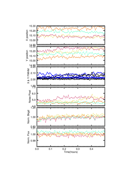
Figure 5.— A zoom in on WASP-14b raw data as a function of time for four random AORs spread throughout the set of observations. Each AOR is color coded with the exception of X and Y FWHM where XFWHM is shown in blue and YFWHM is shown in black. . See §5.2 for more details.

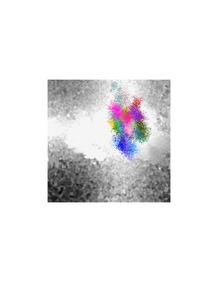
Figure 6.— Greyscale image of the gain variations within a single pixel at the center of the subarray. The centroid positions of WASP-14b snapshot AORs are shown in the same color as the other WASP-14b figures. See §5.2 for more details.

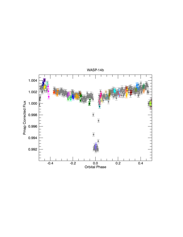
Figure 7.— Final Photometry of WASP-14b. Gray points show our reduction of the continuous staring mode data. Colored points show the snapshot data. All have been binned on the same timescale and normalized to the level in secondary eclipse. Zoom-ins on the transit and eclipse are shown in Figure 14. See §5.3 for more details.

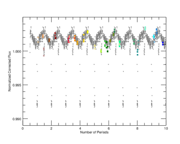
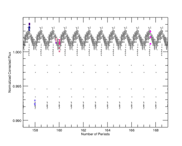
Figure 8.— Flux vs. Time over the 1 year of snapshot observations. The x-axis is in number of periods since the first snapshot observation. Gray points are phased continuous staring mode observations repeated over many periods. Colored points are the snapshot data. Binning is the same for all data. See §5.3 for more details.

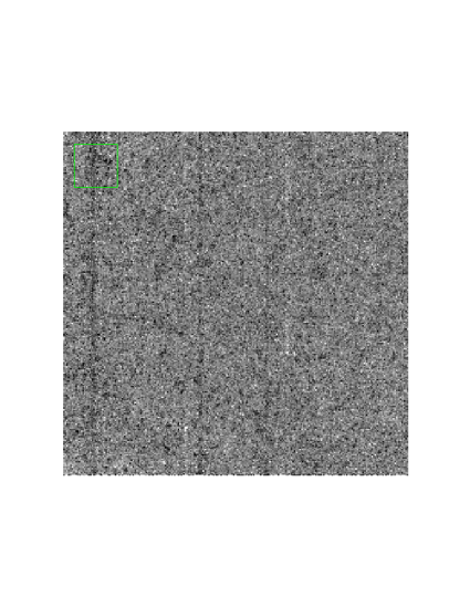
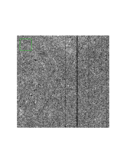
Figure 9.— Left: Median Stack of 80 images taken after a set of snapshot observations with full array frame time of 6s. Right: Median stack of 10 images taken after a different snapshot with full array frame time of 0.4s. The green squares show the location of the subarray field of view. There are clearly negative (more darkly colored) persistent images in the subarray field of view in one of these median stacks and not obviously in the other. The darkly colored vertical stripes are persistent images from a column-wise effect known as column pull-down. The diagonal latent in the right side of the figure is a slew latent where the telescope must have slewed across a bright star at some time prior to these observations. See §6.1.1 for more details.

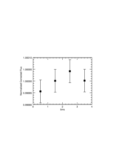
Figure 10.— Corrected flux as a function of time. Fluxes for all 46 snapshot AORs have been binned together. Time is binned into 4 sections to look for trends as a function of time. Y-scale range is 0.02%. There is no electronic ramp from the beginning to the end of the snapshot observations to within 50-100ppm, which is well below our phase curve amplitude signal. See §5.5 for more details.

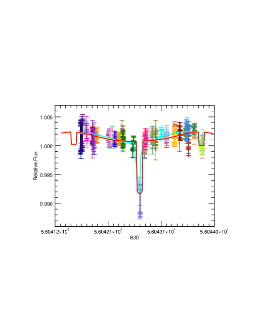
Figure 11.— Fits to the snapshot and continuous staring mode datasets. Data are binned roughly by 64 photometry points. The red line is the fit from this paper to the pmap reduction of the continuous staring mode data, the cyan line is the fit to the snapshot data, and the yellow line is the Wong et al. (2015b) fit to their reduction of the continuous staring mode data(practically indistinguishable from the red line). The cyan line fit to the snapshot data is slightly irregular at transit and eclipse because there isn’t enough data in ingress and egress to provide a smooth fit. An extra 0.01% has been added to the error bars of all data in the AORs which we know are effected by latent images(most notably those in transit). See §6.2 for more details.

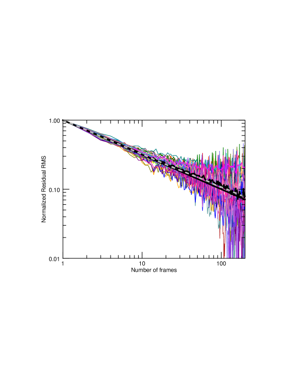
Figure 12.— Normalized Residual RMS versus binning size in number of frames on the bottom and minutes on the top. Each colored line represents a single AOR. Because our observations are only 30 min long, the RMS measurement has a lot of scatter in it at binning scales greater than a few minutes. The straight solid black line is poisson noise. The gray dashed line is the same measurement for the continuous staring mode data taken from Wong et al. (2015b). The squiggly black line is the median over all snapshots. See §6.3.1 for more details.

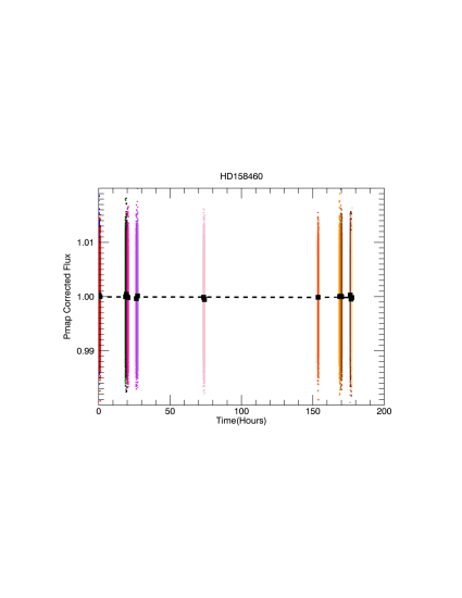
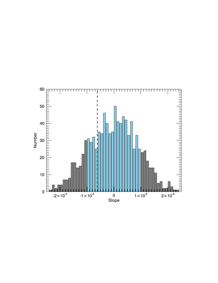
Figure 13.— Snapshots of a calibration star. Left: Light curve of a calibration star where each AOR is shown both unbinned with colored points and as a single binned black square. Right: A monte carlo simulation of possible slopes of fitted lines to this data set. The dashed line shows the chi-squared fit to the actual snapshot observations from the left plot. FWHM of a gaussian fit to the histogram is indicated by a change in color from gray to blue. Snapshot observations are within one sigma of a flat light curve. See §6.3.2 for more details.

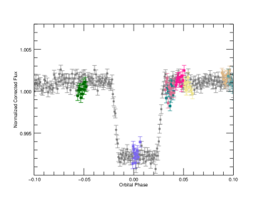
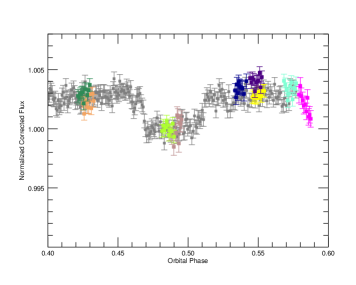
Figure 14.— Comparison of the the transit (left) and secondary eclipse (right) depths between snapshot and continuous staring mode data reduced in the same way. Gray points are the continuous staring mode data, colored points are the snapshot data. Both plots have been normalized to the eclipse level. See §6.5 for more details.

References

- Ballard et al. (2010) Ballard, S., Charbonneau, D., Deming, D., et al. 2010, PASP, 122, 1341
- Blecic et al. (2013) Blecic, J., Harrington, J., Madhusudhan, N., et al. 2013, ApJ, 779, 5
- Burrows et al. (2008) Burrows, A., Budaj, J., & Hubeny, I. 2008, ApJ, 678, 1436
- Burrows et al. (2010) Burrows, A., Rauscher, E., Spiegel, D. S., & Menou, K. 2010, ApJ, 719, 341
- Burrows et al. (2006a) Burrows, A., Sudarsky, D., & Hubeny, I. 2006a, ApJ, 650, 1140
- Burrows et al. (2006b) —. 2006b, ApJ, 650, 1140
- Campo et al. (2011) Campo, C. J., Harrington, J., Hardy, R. A., et al. 2011, ApJ, 727, 125
- Charbonneau et al. (2005a) Charbonneau, D., Allen, L. E., Megeath, S. T., et al. 2005a, ApJ, 626, 523
- Charbonneau et al. (2005b) —. 2005b, ApJ, 626, 523
- Ciardi et al. (2011) Ciardi, D. R., von Braun, K., Bryden, G., et al. 2011, AJ, 141, 108
- Cooper & Showman (2005) Cooper, C. S., & Showman, A. P. 2005, ApJ, 629, L45
- Cowan & Agol (2008) Cowan, N. B., & Agol, E. 2008, ApJ, 678, L129
- Cowan & Agol (2011) —. 2011, ApJ, 726, 82
- Cowan et al. (2007a) Cowan, N. B., Agol, E., & Charbonneau, D. 2007a, MNRAS, 379, 641
- Cowan et al. (2007b) —. 2007b, MNRAS, 379, 641
- Cowan et al. (2012) Cowan, N. B., Machalek, P., Croll, B., et al. 2012, ApJ, 747, 82
- Crossfield et al. (2012a) Crossfield, I. J. M., Barman, T., Hansen, B. M. S., Tanaka, I., & Kodama, T. 2012a, ApJ, 760, 140
- Crossfield et al. (2010) Crossfield, I. J. M., Hansen, B. M. S., Harrington, J., et al. 2010, ApJ, 723, 1436
- Crossfield et al. (2012b) Crossfield, I. J. M., Knutson, H., Fortney, J., et al. 2012b, ApJ, 752, 81
- Deming et al. (2005) Deming, D., Seager, S., Richardson, L. J., & Harrington, J. 2005, Nature, 434, 740
- Deming et al. (2011) Deming, D., Knutson, H., Agol, E., et al. 2011, ApJ, 726, 95
- Deming et al. (2015) Deming, D., Knutson, H., Kammer, J., et al. 2015, ApJ, 805, 132
- Demory et al. (2013) Demory, B.-O., de Wit, J., Lewis, N., et al. 2013, ApJ, 776, L25
- Ehrenreich & Désert (2011) Ehrenreich, D., & Désert, J.-M. 2011, A&A, 529, A136
- Fazio et al. (2004) Fazio, G. G., Hora, J. L., Allen, L. E., et al. 2004, ApJS, 154, 10
- Fortney et al. (2006) Fortney, J. J., Cooper, C. S., Showman, A. P., Marley, M. S., & Freedman, R. S. 2006, ApJ, 652, 746
- Fortney et al. (2008) Fortney, J. J., Lodders, K., Marley, M. S., & Freedman, R. S. 2008, ApJ, 678, 1419
- Grillmair et al. (2008) Grillmair, C. J., Burrows, A., Charbonneau, D., et al. 2008, Nature, 456, 767
- Harrington et al. (2006) Harrington, J., Hansen, B. M., Luszcz, S. H., et al. 2006, Science, 314, 623
- Heng & Showman (2015) Heng, K., & Showman, A. P. 2015, Annual Review of Earth and Planetary Sciences, 43, 509
- Ingalls et al. (2012) Ingalls, J. G., Krick, J. E., Carey, S. J., et al. 2012, in Society of Photo-Optical Instrumentation Engineers (SPIE) Conference Series, Vol. 8442, Society of Photo-Optical Instrumentation Engineers (SPIE) Conference Series
- Johnson et al. (2009) Johnson, J. A., Winn, J. N., Albrecht, S., et al. 2009, PASP, 121, 1104
- Joshi et al. (2009) Joshi, Y. C., Pollacco, D., Collier Cameron, A., et al. 2009, MNRAS, 392, 1532
- Kataria et al. (2013) Kataria, T., Showman, A. P., Lewis, N. K., et al. 2013, ApJ, 767, 76
- Knutson et al. (2009a) Knutson, H. A., Charbonneau, D., Burrows, A., O’Donovan, F. T., & Mandushev, G. 2009a, ApJ, 691, 866
- Knutson et al. (2009b) Knutson, H. A., Charbonneau, D., Cowan, N. B., et al. 2009b, ApJ, 703, 769
- Knutson et al. (2010) Knutson, H. A., Howard, A. W., & Isaacson, H. 2010, ApJ, 720, 1569
- Knutson et al. (2007a) Knutson, H. A., Charbonneau, D., Allen, L. E., et al. 2007a, Nature, 447, 183
- Knutson et al. (2007b) —. 2007b, Nature, 447, 183
- Knutson et al. (2009c) Knutson, H. A., Charbonneau, D., Cowan, N. B., et al. 2009c, ApJ, 690, 822
- Knutson et al. (2012) Knutson, H. A., Lewis, N., Fortney, J. J., et al. 2012, ApJ, 754, 22
- Knutson et al. (2014) Knutson, H. A., Fulton, B. J., Montet, B. T., et al. 2014, ApJ, 785, 126
- Krick et al. (2015) Krick, J., Ingalls, J., Carey, S., et al. 2015, IRAC High Precision Photometry Website, http://irachpp.spitzer.caltech.edu
- Krick et al. (2012) Krick, J. E., Glaccum, W. J., Carey, S. J., et al. 2012, ApJ, 754, 53
- Krick et al. (2009) Krick, J. E., Surace, J. A., Thompson, D., et al. 2009, ApJS, 185, 85
- Laughlin et al. (2009) Laughlin, G., Deming, D., Langton, J., et al. 2009, Nature, 457, 562
- Lewis et al. (2010) Lewis, N. K., Showman, A. P., Fortney, J. J., et al. 2010, ApJ, 720, 344
- Lewis et al. (2013) Lewis, N. K., Knutson, H. A., Showman, A. P., et al. 2013, ApJ, 766, 95
- Madhusudhan (2012) Madhusudhan, N. 2012, ApJ, 758, 36
- Maxted et al. (2013) Maxted, P. F. L., Anderson, D. R., Doyle, A. P., et al. 2013, MNRAS, 428, 2645
- Menou & Rauscher (2010) Menou, K., & Rauscher, E. 2010, ApJ, 713, 1174
- Mighell (2005) Mighell, K. J. 2005, MNRAS, 361, 861
- Nadaraya (2006) Nadaraya, E. A. 2006, Theory of Probability & Its Applications, 9, 141
- Paulson et al. (2004) Paulson, D. B., Cochran, W. D., & Hatzes, A. P. 2004, AJ, 127, 3579
- Perez-Becker & Showman (2013) Perez-Becker, D., & Showman, A. P. 2013, ApJ, 776, 134
- Reach et al. (2005) Reach, W. T., Megeath, S. T., Cohen, M., et al. 2005, PASP, 117, 978
- Santos et al. (2000) Santos, N. C., Mayor, M., Naef, D., et al. 2000, A&A, 361, 265
- Schwartz & Cowan (2015) Schwartz, J. C., & Cowan, N. B. 2015, MNRAS, 449, 4192
- Showman et al. (2015) Showman, A. P., Lewis, N. K., & Fortney, J. J. 2015, ApJ, 801, 95
- Sing & López-Morales (2009) Sing, D. K., & López-Morales, M. 2009, A&A, 493, L31
- Spiegel et al. (2009) Spiegel, D. S., Silverio, K., & Burrows, A. 2009, ApJ, 699, 1487
- Stevenson et al. (2012) Stevenson, K. B., Harrington, J., Fortney, J. J., et al. 2012, ApJ, 754, 136
- Stevenson et al. (2014) Stevenson, K. B., Désert, J.-M., Line, M. R., et al. 2014, Science, 346, 838
- Thrastarson & Cho (2010) Thrastarson, H. T., & Cho, J. Y. 2010, ApJ, 716, 144
- Todorov et al. (2012) Todorov, K. O., Deming, D., Knutson, H. A., et al. 2012, ApJ, 746, 111
- Todorov et al. (2013) —. 2013, ApJ, 770, 102
- Watson (1964) Watson, G. S. 1964, Sankhyā: The Indian Journal of Statistics, Series A (1961-2002), 26, 359
- Werner et al. (2004) Werner, M. W., Roellig, T. L., Low, F. J., et al. 2004, ApJS, 154, 1
- Wong et al. (2015a) Wong, I., Knutson, H. A., Kataria, T., et al. 2015a, ArXiv e-prints, arXiv:1512.09342
- Wong et al. (2015b) Wong, I., Knutson, H. A., Lewis, N. K., et al. 2015b, ApJ, 811, 122
- Zellem et al. (2014) Zellem, R. T., Lewis, N. K., Knutson, H. A., et al. 2014, ApJ, 790, 53
- Zhao et al. (2012) Zhao, M., Monnier, J. D., Swain, M. R., Barman, T., & Hinkley, S. 2012, ApJ, 744, 122