Holographic Fermi Liquids in a Spontaneously Generated Lattice

Abstract

We discuss fermions in a spontaneously generated holographic lattice background. The lattice structure at the boundary is generated by introducing a higher-derivative interaction term between a $U(1)$ gauge field and a scalar field. We solve the equations of motion below the critical temperature at which the lattice forms, and analyze the change in the Fermi surface due to the lattice. The fermion band structure is found to exhibit a gap due to lattice effects.

I Introduction

The normal state of copper oxide high-temperature superconductors has been found to possess anomalous thermal and optical conductivities and electrical resistivity. An explanation of this behavior was put forward in Abrahams , citing that over a wide range of momenta, there exist excitations contributing to both the charge and spin polarizability. The retarded one-particle self-energy accounting for the exchange of charge and spin fluctuations were found to be quite different than that of a conventional Fermi liquid. The spectral function $A(k,\omega)$ is much broader and carries substantially more weight in the wings because of an $\omega^{-1}$ tail. The behavior is referred to as a marginal Fermi liquid.

The formation of a marginal Fermi liquid in the normal phase of the superconductor implies that the quasiparticle excitations are unstable. A way to stabilize the quasiparticles was proposed in Faulkner:2009am by employing the gauge/gravity duality in which strongly-coupled phenomena were studied using dual, weakly-coupled gravitational systems Maldacena:1997re ; Gubser:2002 ; Witten:1998 . A coupling was introduced between the fermion and the condensate formed in the superconducting phase capable of stabilizing the quasiparticles with a gap. A similar investigation was carried out in Gubser:2009dt , where the effect of a background, zero-temperature superconducting anti-de Sitter domain wall was considered.

A system with interacting bosonic and fermionic degrees of freedom at finite density was considered holographically in Nitti:2014fsa . By computing the two-point Green function of the boundary fermionic operator, it was shown that in the presence of the charged scalar condensate, the dual field theory exhibited electron-like and/or hole-like Fermi surfaces. Compared to fluid-only solutions, the presence of the scalar condensate destabilized the Fermi surfaces with lowest Fermi momenta and a gap appeared.

Recently, in the context of holography, lattice effects on the Fermi surfaces have garnered interest. The study of condensed matter systems on the boundary in the presence of a lattice requires a gravitational background lacking spatial homogeneity. Lattice effects were introduced in a strongly-coupled system of fermions at a finite density in LSSZ:2012 . The holographic dual consisted of fermions in the presence of a Reissner-Nordström-anti-de Sitter black hole with the lattice effect encoded by periodic modulation of the chemical potential with a wavelength on the order of the Fermi momentum. In the marginal Fermi liquid regime a gap was formed due to the interaction between different excitation levels. The spectral weight remained small but non-zero inside of the gap. This behavior is described as a “pseudogap” to differentiate from that of a band gap with identically zero spectral weight.

A Dirac field in the presence of a holographic lattice was studied in Ling:2013fl . In the low temperature limit, the Fermi surface was modified by lattice effects from a circle to an ellipse. The behavior was attributed to the presence of quasiparticles made more massive by renormalization effects due to the lattice. Additionally, a pseudogap band structure was found at the intersection of the Fermi surface and the Brillouin zone boundary.

The holographic lattice background may be constructed by introducing a scalar field with periodic boundary conditions along a spatial direction or by employing a periodic chemical potential for the scalar potential of the gauge field. In most of the cases, a spatial inhomogeneity is introduced perturbatively Maeda:2011pk ; LSSZ:2012 ; Aperis:2010cd ; Flauger:2010tv ; Hutasoit:2012ib ; Erdmenger:2013zaa ; Donos:2013eha . Recently, the authors in Horowitz:2012ky and Horowitz:2012gs constructed some spatially inhomogeneous but periodic gravitational backgrounds by fully solving the coupled partial differential equations numerically with the Einstein-DeTurck method. In Alsup:2013kda , it was shown that by turning on a higher-derivative interaction term between a $U(1)$ gauge field and a scalar field, the scalar field spontaneously develops a spatially-dependent profile. Through backreaction, the charge density spontaneously developed spatial inhomogeneity.

In this work, we introduce a Dirac field in a gravity background. A spatial inhomogeneity and subsequently a modulated charge density are spontaneously generated, in the spirit of Alsup:2013kda . We study the boundary lattice effects on the Fermi surface by analytically solving, up to second order, the backreacted geometry and Dirac equation in the bulk. The structure of the Fermi surface and a pseudogap behavior of the fermions are analyzed with the Green function behavior of the Dirac field.

The paper is organized as follows. In Section II, we perturbatively study the numerical and analytic solutions of a holographic system with spontaneously generated inhomogeneous phases introduced by higher derivative couplings. In Section III, we introduce a Dirac field into the holographic lattice system. We analyze the lattice effects on the Fermi surface by calculating the spectral function of the system. To this end, we perturbatively solve the Dirac equations in the periodic background at small but finite temperature. We discuss the supporting numerical results for the spectral function at the critical temperature (zeroth order) in Section IV. In Section V we present the solutions below the critical temperature, the first order in Section V.1, and the second order of perturbation in Section V.2. In Section V.3 we discuss the generation of the pseudogap. Finally, in Section VI, we discuss the results of this study and present an outlook for future studies.

II General Formalism

We begin by considering a holographic system consisting of a $U(1)$ gauge field $A_{\mu}$, of field strength $F_{\mu\nu}=\partial_{\mu}A_{\nu}-\partial_{\nu}A_{\mu}$, and of a scalar field $\phi$ of charge $q$ under the $U(1)$ group of the gauge field, having mass $m$. Later, a Dirac field with mass $m_{f}$ and charge $q_{f}$ will be added to the system. The $AdS$ spacetime geometry of the bulk where these fields live has a negative cosmological constant of $\Lambda=-3/L^{2}$.

We consider the following action

$$S=\int d^{4}x\sqrt{-g}\mathcal{L}~{},\ \ \ \ \mathcal{L}=\frac{R+6/L^{2}}{16\pi G}-\frac{1}{4}F_{\mu\nu}F^{\mu\nu}-(D_{\mu}\phi)^{*}D^{\mu}\phi-m^{2}|\phi|^{2}~{},$$ (1)

with $D_{\mu}\phi=\partial_{\mu}\phi-iqA_{\mu}\phi$. In the rest of this paper, we shall choose units so that $16\pi G=L=1$.

Following Alsup:2013kda , we introduce higher derivative terms that lead to spatial inhomogeneity in the boundary theory. These terms were shown to lead to a holographic lattice structure on the boundary,

$$\mathcal{L}_{\mathrm{int}}=\eta\mathcal{G}^{\mu\nu}(D_{\mu}\phi)^{\ast}D_{\nu}\phi-\eta^{\prime}|D_{\mu}\mathcal{G}^{\mu\nu}D_{\nu}\phi|^{2}\ ,$$ (2)

where $\mathcal{G}_{\mu\nu}=F_{\mu\rho}{F_{\nu}}^{\rho}-\frac{1}{2}g_{\mu\nu}F^{\rho\sigma}F_{\rho\sigma}$.

The action (1) with the additional interaction term (2) gives the Einstein equations

$$G_{\mu\nu}-3g_{\mu\nu}=\frac{1}{2}T_{\mu\nu}~{},$$ (3)

where $T_{\mu\nu}$ is the stress-energy tensor,

$$T_{\mu\nu}=T_{\mu\nu}^{(EM)}+T_{\mu\nu}^{(\phi)}+\Theta_{\mu\nu}~{},$$ (4)

and the gauge, scalar, and interaction contributions, respectively, may be written as

$$T_{\mu\nu}^{(EM)} = F_{\mu\rho}{F_{\nu}}^{\rho}-\frac{1}{4}g_{\mu\nu}F^{\rho\sigma}F_{\rho\sigma}~{},$$

$$T_{\mu\nu}^{(\phi)} = (D_{\mu}\phi)^{\ast}D_{\nu}\phi+D_{\mu}\phi(D_{\nu}\phi)^{\ast}-g_{\mu\nu}(D_{\alpha}\phi)^{\ast}D^{\alpha}\phi-m^{2}g_{\mu\nu}|\phi|^{2}~{},$$

$$\Theta_{\mu\nu} = \frac{2}{\sqrt{-g}}\frac{\delta\mathcal{L}_{\mathrm{int}}}{\delta g^{\mu\nu}}~{}.$$ (5)

The Maxwell equations are obtained by varying the Lagrangian with respect to $A_{\mu}$ as

$$\nabla_{\mu}F^{\mu\nu}=J^{\nu}+\mathcal{J}^{\nu}\ ,$$ (6)

where the current, contains scalar and interaction contributions, respectively,

$$J_{\mu}=iq\left[\phi^{\ast}D_{\mu}\phi-(D_{\mu}\phi)^{\ast}\phi\right]~{},\ \ \mathcal{J}_{\mu}=\frac{1}{\sqrt{-g}}\frac{\delta\mathcal{L}_{\mathrm{int}}}{\delta A^{\mu}}~{}.$$ (7)

Finally, varying the Lagrangian with respect to the scalar field gives the scalar equation of motion as

$$D_{\mu}D^{\mu}\phi-m^{2}\phi=\eta D_{\mu}\left(\mathcal{G}^{\mu\nu}D_{\nu}\phi\right)+\eta^{\prime}D_{\rho}(\mathcal{G}^{\mu\rho}D_{\mu}(D_{\nu}(\mathcal{G}^{\nu\sigma}D_{\sigma}\phi)))~{}.$$ (8)

To capture the lattice effects, we consider the following metric ansatz

$$\begin{split}ds^{2}=&\frac{1}{z^{2}}\Big{[}-h(z)Q_{tt}(x,z)dt^{2}+\frac{Q_{zz}(x,z)dz^{2}}{h(z)}\\ &\ \ \ \ \ +Q_{xx}(x,z)(dx+z^{2}Q_{xz}(x,z)dz)^{2}+Q_{yy}(x,z)dy^{2}\Big{]}~{},\end{split}$$ (9)

where $h(z)$ is a fixed function, conveniently separated from the rest of $g_{tt}$, defined as

$$h(z)=1-\left(1+\frac{\mu_{0}^{2}}{4}\right)z^{3}+\frac{\mu_{0}^{2}}{4}z^{4}~{}.$$ (10)

The required boundary conditions at the horizon and boundary are, respectively,

$$Q_{tt}(x,1)=Q_{zz}(x,1)~{},$$ (11)

and

$$Q_{tt}(x,0)=Q_{zz}(x,0)=Q_{xx}(x,0)=Q_{yy}(x,0)=1~{},~{}Q_{xz}(x,0)=0~{},~{}A_{t}(x,0)=\mu~{},$$ (12)

where we consider the system held under constant chemical potential $\mu$.

Notice that we have chosen coordinates in which the horizon is fixed at $z=1$. This fixes the overall scale of the system arbitrarily. Thus, the results ought to be reported in the form of dimensionless quantities. For example. the dimensionless temperature is given by

$$\frac{T}{\mu}=\frac{12-\mu_{0}^{2}}{16\pi\mu}~{},$$ (13)

where $\mu=\mu_{0}$ above the critical temperature (in the absence of condensation of the scalar field). Below the critical temperature, $\mu$, measured in units of the radius of the horizon, increases.

The solutions of the equations of motion have the same form as found in Alsup:2013kda at or above the critical temperature. In particular, the scalar field right below the critical temperature is not homogeneous, but of the form

$$\phi(x,z)=\frac{\left<\mathcal{O}\right>}{\sqrt{2}}z^{\Delta}F(z)\cos(kx)~{},\ \ F(0)=1$$ (14)

leading to the formation of a one-dimensional lattice, where $\Delta$ is the scaling dimension of the dual boundary operator $\mathcal{O}$.

Next, we will solve the equations of motion below the critical temperature with the ansatz (9). To this end, we expand all the fields in the order parameter

$$\xi=\frac{\langle\mathcal{O}\rangle}{\sqrt{2}}~{},$$ (15)

as

$$Q_{tt}(x,z) = 1+\xi^{2}Q_{tt}^{1}(x,z)+\mathcal{O}(\xi^{4})~{},$$

$$Q_{zz}(x,z) = 1+\xi^{2}Q_{zz}^{1}(x,z)+\mathcal{O}(\xi^{4})~{},$$

$$Q_{xx}(x,z) = 1+\xi^{2}Q_{xx}^{1}(x,z)+\mathcal{O}(\xi^{4})~{},$$

$$Q_{xz}(x,z) = \xi^{2}Q_{xz}^{1}(x,z)+\mathcal{O}(\xi^{4})~{},$$

$$Q_{yy}(x,z) = 1+\xi^{2}Q_{yy}^{1}(x,z)+\mathcal{O}(\xi^{4})~{},$$

$$\phi(x,z) = \xi\phi^{0}(x,z)+\xi^{3}\phi^{1}(x,z)+\mathcal{O}(\xi^{5})~{},$$

$$A_{t}(x,z) = (1-z)\left[A_{t}^{0}(z)+\xi^{2}A_{t}^{1}(z,x)+\mathcal{O}(\xi^{4})\right]~{},$$ (16)

where $\phi^{0}$, and $A_{t}^{0}$ are defined at the critical temperature $T_{c}$. The chemical potential (in units of the horizon radius) is given by

$$\mu\equiv A_{t}(x,0)=\mu_{0}+\xi^{2}\mu_{1}+\mathcal{O}(\xi^{2})\ \ ,\ \ \ \ \mu_{0}=A_{t}^{0}(0)\ \ ,\ \ \ \ \mu_{1}=A_{t}^{1}(x,0)~{}.$$ (17)

It should be emphasized that $\mu$ is a constant (independent of $x$), i.e., we impose the boundary condition that $A_{t}(x,0)$ is a (fixed) constant. Dependence of the system on $x$ will be generated spontaneously.

The perturbative fields may be expanded in Fourier modes. At each given order of the parameter $\xi$, only a finite number of modes of the various fields are generated. At first order, i.e., $\mathcal{O}(\xi^{2})$, we have only the $0$ and $2k$ Fourier modes for the metric and gauge field functions, and $k$ and $3k$ modes for the scalar field,

$$Q_{tt}^{1}(x,z) = Q_{tt}^{1,0}(z)+Q_{tt}^{1,1}(z)\cos 2kx~{},$$

$$Q_{zz}^{1}(x,z) = Q_{zz}^{1,0}(z)+Q_{zz}^{1,1}(z)\cos 2kx~{},$$

$$Q_{xx}^{1}(x,z) = Q_{xx}^{1,0}(z)+Q_{xx}^{1,1}(z)\cos 2kx~{},$$

$$Q_{xz}^{1}(x,z) = Q_{xz}^{1,0}(z)+Q_{xz}^{1,1}(z)\sin 2kx~{},$$

$$Q_{yy}^{1}(x,z) = Q_{yy}^{1,0}(z)+Q_{yy}^{1,1}(z)\cos 2kx~{},$$

$$A_{t}^{1}(x,z) = A_{t}^{1,0}(z)+A_{t}^{1,1}(z)\cos 2kx~{},$$

$$\phi^{1}(x,z) = \phi^{1,0}(z)\cos kx+\phi^{1,1}(z)\cos 3kx~{}.$$ (18)

These modes can be obtained by solving the system of Einstein-Maxwell-scalar field equations. Details can be found in Appendix A.

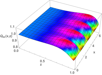
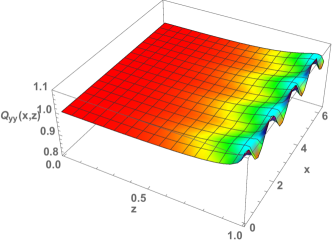
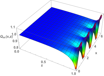
Figure 1: Numerical solutions for the metric functions, $Q_{tt}(x,z)$, $Q_{zz}(x,z)$, $Q_{xx}(x,z)$, and $Q_{yy}(x,z)$, for $\frac{\eta}{\mu^{2}}=0.41$, $\frac{\eta^{\prime}}{\mu^{4}}=0.005$, $q=0$, $\Delta=1$.

The charge density of the system can be determined through the dimensionless quantity

$$\frac{\rho}{\mu^{2}}=-\frac{\partial_{z}\left[(1-z)A_{t}(x,z)\right]|_{z=0}}{[A_{t}(x,0)]^{2}}~{}.$$ (19)

In Fig. 1, we plot the modes of the metric functions, $Q_{tt}(x,z)$, $Q_{zz}(x,z)$, $Q_{xx}(x,z)$, and $Q_{yy}(x,z)$, while the charge density of the system is shown in Fig. 2. As can be seen in these figures, non-trivial $x-$spatially anisotropic profiles of the fields are developing below the critical temperature. The same behavior is also observed in the profile of the scalar field, shown in Fig. 3. In Fig. 2, the charge density is shown to be spatially modulated, indicating a holographic lattice structure below $T_{c}$. We observed that while keeping $\xi$ fixed and varying the other parameters, the spatial modulation varied as well. For example, as the critical temperature $T_{c}$ was lowered, the magnitude of the spatial modulation decreased.

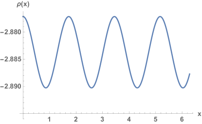
Figure 2: The charge density of the system for $\frac{\eta}{\mu_{0}^{2}}=0.41$, $\frac{\eta^{\prime}}{\mu_{0}^{4}}=0.005$, $q=0$, $\Delta=1$, and $\xi=0.1$.

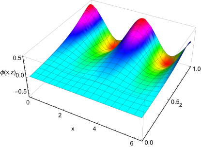
Figure 3: The scalar field of the system with first order contributions included for parameters $\frac{\eta}{\mu_{0}^{2}}=0.41$, $\frac{\eta^{\prime}}{\mu_{0}^{4}}=0.005$, $q=0$, $\Delta=1$, and $\xi=0.1$.

In summary, we have a perturbative, backreacted solution up to first order in $\xi^{2}$ for the Einstein-Maxwell-scalar equations. Next-to-leading-order effects can be systematically introduced, but will not be needed for our purposes. Our focus is the behavior of the fermions and next-to-leading-order corrections to the other fields contribute negligibly to the leading order behavior of the fermionic fields.

III The Dirac Equation

In this section we introduce a Dirac spinor field $\Psi(z,t,x,y)$ with mass $m_{f}$ and charge $q_{f}$, in addition to the scalar, gauge, and gravitational fields introduced in the previous section. The bulk action for the Dirac field is given by

$$S_{D}=i\int d^{4}x\sqrt{-g}{\bar{\Psi}}(\Gamma^{a}\mathcal{D}_{a}-m_{f})\Psi~{},$$ (20)

where $\Gamma^{a}=(e_{\mu})^{a}\Gamma^{\mu}$ with a set of orthogonal normal vector bases $(e_{\mu})^{a}$ and $\Gamma^{\mu}$ the Dirac gamma matrices. The covariant derivative $\mathcal{D}_{a}$ is defined as

$$\mathcal{D}_{a}=\partial_{a}+\frac{1}{4}(\omega_{\mu\nu})_{a}\Gamma^{\mu\nu}-iq_{f}A_{a}~{},$$ (21)

with $\Gamma^{\mu\nu}=\frac{1}{2}[\Gamma^{\mu},\Gamma^{\nu}]$, and $(\omega_{\mu\nu})_{a}=(e_{\mu})_{b}\nabla_{a}(e_{\nu})^{b}$ are the spin connection 1-forms. The indices $a$, $b$ denote tangent space, and the $\mu,\nu$ indices denote the boundary directions. The gamma matrices satisfy the Clifford algebra $\{\Gamma^{a},\Gamma^{b}\}=2\eta^{ab}$, and $\Gamma_{ab}=\frac{1}{2}[\Gamma_{a},\Gamma_{b}]$.

From the action (20) with the metric (9), the Dirac equation is of the form

$$\begin{split}&-\sqrt{\frac{h}{Q_{zz}}}\Gamma^{4}\partial_{z}\Psi+\frac{1}{\sqrt{hQ_{tt}}}\Gamma^{1}\left(\partial_{t}-iq_{f}A_{t}\right)\Psi+\frac{1}{\sqrt{Q_{xx}}}\Gamma^{2}\partial_{x}\Psi+\frac{1}{\sqrt{Q_{yy}}}\Gamma^{3}\partial_{y}\Psi-\frac{m_{f}}{z}\Psi\\ &+\frac{1}{4\sqrt{Q_{xx}}}\partial_{x}\ln\frac{Q_{tt}Q_{zz}Q_{yy}}{z^{6}}\Gamma^{2}\Psi-\frac{1}{4}\sqrt{\frac{h}{Q_{zz}}}\partial_{z}\ln\frac{hQ_{tt}Q_{xx}Q_{yy}}{z^{6}}\Gamma^{4}\Psi=0~{}.\end{split}$$ (22)

We choose the basis

$$\Gamma^{1}=\begin{pmatrix}i\sigma^{1}&0\\ 0&i\sigma^{1}\end{pmatrix},\ \ \ \Gamma^{2}=\begin{pmatrix}-\sigma^{2}&0\\ 0&\sigma^{2}\end{pmatrix},\ \ \ \Gamma^{3}=\begin{pmatrix}0&\sigma^{2}\\ \sigma^{2}&0\end{pmatrix},\ \ \ \Gamma^{4}=\begin{pmatrix}-\sigma^{3}&0\\ 0&-\sigma^{3}\end{pmatrix}$$ (23)

for the gamma matrices of the (3+1)-dimensional bulk theory, and the following ansatz for the spinor fields

$$\Psi=\left(\frac{hQ_{tt}Q_{xx}Q_{yy}}{z^{6}}\right)^{-\frac{1}{4}}e^{-i\omega t+i(k_{x}x+k_{y}y)}\psi\ \ ,\ \ \ \ \psi=\begin{pmatrix}\psi_{+}\\ \psi_{-}\end{pmatrix}\ \ ,\ \ \ \ \psi_{\pm}=\begin{pmatrix}\psi_{\pm 1}\\ \psi_{\pm 2}\end{pmatrix}~{}.$$ (24)

We have a holographic lattice structure in the $x$ dimension. Therefore, we can expand the spinor fields, according to the Bloch theorem, as

$$\psi_{\alpha s}(x,z)=\sum_{l=0,\pm 1,\pm 2,\dots}\psi_{\alpha s}^{l}(z)e^{2ilkx}~{},$$ (25)

where $\alpha=\pm,s=1,2$.

Upon substituting (25) into the Dirac equation (22), we obtain a set of coupled equations with infinitely many fields, corresponding to the full range of $l=0,\pm 1,\pm 2,\dots,\pm\infty$. Our aim is to calculate the retarded Green function and the spectral function to characterize the fermionic system. This is equivalent to measuring the spectral function by Angular Resolved Photoemission Spectroscopy (ARPES), as discussed in Faulkner:2010da . To this end, we will numerically and analytically solve the equations using perturbation theory at small but finite temperature, and compare the behavior of these solutions to those above the critical temperature.

The backreaction contribution of the scalar field, gauge field, and metric are of first order in $\xi$ for our expansion (16). To solve the Dirac equation for the spinor field, we expand in $\xi$ up to second order as

$$\psi_{\alpha s}^{l}(z)=\psi_{\alpha s}^{0,l}+\xi^{2}\psi_{\alpha s}^{1,l}+\xi^{4}\psi_{\alpha s}^{2,l}+\mathcal{O}(\xi^{6})~{}.$$ (26)

Near the horizon, we have ingoing boundary conditions,

$$\begin{pmatrix}\psi_{\pm 1}\\ \psi_{\pm 2}\end{pmatrix}\sim\begin{pmatrix}1\\ -i\end{pmatrix}(1-z)^{-\frac{i\omega}{4\pi T}}~{},$$ (27)

To implement them, we write

$$\psi_{\alpha s}(z)=(1-z)^{-\frac{i\omega}{4\pi T}}F_{\alpha s}(z)~{},$$ (28)

where $F_{\alpha 1}=1$ and $F_{\alpha 2}=-i$, at $z=1$.

For fixed $\alpha,l$, we obtain a unique solution by setting $\psi_{\beta s}^{0,l^{\prime}}=0$, for all $(\beta,l^{\prime})\neq(\alpha,l)$. Physically, this means that at the critical temperature, we have a single mode labeled by $\alpha,l$. At higher orders in $\xi$, i.e., below the critical temperature, more modes are generated.

At the AdS boundary ($z\to 0$), the mode of the solution to the Dirac equation labeled by $\beta,l^{\prime}$ asymptotes to

$$\psi_{\beta}^{l^{\prime}}(z)\approx A_{\alpha\beta}^{ll^{\prime}}\,z^{-m_{f}}\begin{pmatrix}0\\ 1\end{pmatrix}+B_{\alpha\beta}^{ll^{\prime}}\,z^{m_{f}}\begin{pmatrix}1\\ 0\end{pmatrix}~{},$$ (29)

where $\alpha,l$ encode the choice of solution at the critical temperature. The retarded Green function can be found from the matrices formed by the coefficients in the asymptotic expansion, through the matrix

$$\mathbf{G}_{R}=\mathbf{BA}^{-1}~{}.$$ (30)

We will solve the Dirac equation up to second order in $\xi^{2}$. To find the explicit form of the retarded Green function from (30), we note that the diagonal elements of the matrix $\mathbf{A}$ have contributions which are $\mathcal{O}(\xi^{0})$ and $\mathcal{O}(\xi^{4})$, whereas the off-diagonal elements are $\mathcal{O}(\xi^{2})$. These follow directly from the Dirac equation. The retarded Green function for the solution labeled by $\alpha,l$ can therefore be written as

$$G_{R}=\left(\mathbf{G}_{R}\right)_{\alpha\alpha}^{ll}=\frac{1}{\det A}\left\{\sum_{\beta=+,-}\left(B_{\alpha\beta}^{ll-1}\Delta_{\alpha\beta}^{ll-1}+B_{\alpha\beta}^{ll+1}\Delta_{\alpha\beta}^{ll+1}\right)+B_{\alpha\alpha}^{ll}\Delta_{\alpha\alpha}^{ll}+\mathcal{O}(\xi^{4})\right\}~{},$$ (31)

where $\Delta_{\alpha\beta}^{ll^{\prime}}$ are the cofactors of the matrix $A$ LSSZ:2012 .

The spectral function is the imaginary part of the diagonal terms of the retarded Green function,

$$A^{l}(\omega,k_{x},k_{y})=\Im\left[\left(G_{R}\right)_{+}^{l}+\left(G_{R}\right)_{-}^{l}\right]~{},$$ (32)

and gives the location of the Fermi surface. Although the Fermi surface is defined at zero temperature, as indicated in Ling:2013fl and BHY2010 , it may be located by searching for a peak in the spectral function $A(\omega,k_{x},k_{y})$ at small frequency $\omega$ and low temperatures.

IV Fermionic solution at the critical temperature

In this section we discuss the physics of the fermionic solution at small but non-zero critical temperature. Here and in subsequent sections, we focus on low frequency modes ($\omega\ll\mu_{0}$), because they determine the macroscopic properties of the system. Results are obtained both analytically and numerically in the low-temperature limit. The Dirac equation at the critical temperature reads

$$\partial_{z}{\psi}^{0,l}_{\alpha s}-i\frac{q_{f}\mu_{0}(1-z)+\omega}{h(z)}\sigma^{2}{\psi}^{0,l}_{\alpha s}+\frac{k_{x}+2kl}{\sqrt{h(z)}}\sigma^{3}{\psi}^{0,l}_{\alpha s}-\frac{k_{y}}{\sqrt{h(z)}}\sigma^{1}\psi^{0,l}_{-\alpha\ 3-s}=0~{},$$ (33)

where $\alpha=\pm$, $s=1,2$, and we have set $m_{f}=0$.

To obtain the analytic solution at low frequencies, we solve the Dirac equation in the near-horizon region ($1-z\ll 1$) and in the far region ($1-z\gg\omega/\mu_{0}$), and then match the two solutions in the overlapping region ($\omega/\mu_{0}\ll 1-z\ll 1$).

In the small temperature limit, the near-horizon region is AdS${}_{2}\times\mathbb{R}^{2}$, and the metric can be written as Faulkner:2009wj

$$ds^{2}=\frac{1}{6u^{2}}\left(-(1-\frac{u^{2}}{u_{0}^{2}})dt^{2}+\frac{du^{2}}{1-\frac{u^{2}}{u_{0}^{2}}}\right)+dx^{2}+dy^{2}$$ (34)

after changing coordinates to $u=\frac{\omega z_{\ast}^{2}}{6(z_{\ast}-z)}$, where $z_{\ast}=\frac{2\sqrt{3}}{\mu_{0}}$. The horizon is at $u_{0}=\frac{\omega z_{\ast}^{2}}{6(z_{\ast}-1)}$ with corresponding temperature $T=1/2\pi u_{0}$, and the $U(1)$ gauge field is given by

$$A_{t}^{0}=\frac{1}{\sqrt{3}}\left(\frac{1}{u}-\frac{1}{u_{0}}\right)~{}.$$ (35)

After performing the $SO(2)$ rotation discussed in Appendix B, it is convenient to express the rotated Dirac field in the near-horizon region as

$$\tilde{\psi}_{\alpha s}^{0,l}=\frac{1}{\sqrt{2}}\left(1-\frac{u^{2}}{u_{0}^{2}}\right)^{-1/4}(1+i\sigma^{1})\tilde{y}_{\alpha s}^{0,l}(u)~{}.$$ (36)

The massless Dirac equation at zeroth order becomes independent of $\omega$,

$$\partial_{u}\tilde{y}_{\alpha s}^{0,l}-\frac{i}{1-\frac{u^{2}}{u_{0}^{2}}}\sigma^{3}\left(1+q_{f}A_{t}^{0}\right)\tilde{y}_{\alpha s}^{0,l}-\frac{\alpha\sqrt{2}k_{l}}{\mu_{0}u\sqrt{1-\frac{u^{2}}{u_{0}^{2}}}}\sigma^{1}\tilde{y}_{\alpha s}^{0,l}$$ (37)

where $k_{l}^{2}=(k_{x}+2kl)^{2}+k_{y}^{2}$. For the upper component of $\tilde{y}_{\alpha s}^{0,l}(u)$, we obtain the second-order equation

$$\mathbf{L}_{2}[\tilde{y}_{\alpha 1}^{0,l}]=0$$ (38)

where

$$\mathbf{L}_{2}[\tilde{y}]\equiv\partial_{u}^{2}\tilde{y}+\frac{1-2\frac{u^{2}}{u_{0}^{2}}}{u(1-\frac{u^{2}}{u_{0}^{2}})}\partial_{u}\tilde{y}+\left[-\frac{\nu_{k_{l}}^{2}}{u^{2}(1-\frac{u^{2}}{u_{0}^{2}})}+\frac{\left(1+q_{f}A_{t}^{0}\right)^{2}-\frac{q_{f}^{2}A_{t}^{0}}{\sqrt{3}}\left(\frac{1}{u_{0}}+\frac{1}{u}\right)-\frac{iq_{f}A_{t}^{0}}{u_{0}}-\frac{i}{u}}{(1-\frac{u^{2}}{u_{0}^{2}})^{2}}\right]\tilde{y}$$ (39)

and we defined

$$\nu_{k_{l}}=\frac{\sqrt{2}}{\mu_{0}}\sqrt{k_{l}^{2}-\frac{q_{f}^{2}\mu_{0}^{2}}{6}}~{}.$$ (40)

The solution satisfying ingoing boundary conditions at the horizon may be expressed in terms of hypergeometric functions (up to an irrelevant normalization constant)

$$\tilde{y}_{\alpha 1}^{0,l} = \left(1+\frac{u_{0}}{u}\right)^{\frac{1}{2}+\frac{iq_{f}}{\sqrt{3}}}\left(\frac{u_{0}^{2}}{u^{2}}-1\right)^{-\frac{iu_{0}}{2}}$$ (41)

$$\times\ {{}_{2}}F_{1}\left(\frac{1}{2}-\nu_{k_{l}}+\frac{iq_{f}}{\sqrt{3}}-iu_{0},\frac{1}{2}+\nu_{k_{l}}+\frac{iq_{f}}{\sqrt{3}}-iu_{0};\frac{1}{2}-iu_{0};\frac{u-u_{0}}{2u}\right)~{}.\ \ \ \ \ \$$

Working similarly, we obtain the lower component of $\tilde{y}_{\alpha}^{0,l}$,

$$\tilde{y}_{\alpha 2}^{0,l} = \left(1+\frac{u_{0}}{u}\right)^{\frac{1}{2}-\frac{iq_{f}}{\sqrt{3}}+\frac{iu_{0}}{2}}\left(\frac{u_{0}}{u}-1\right)^{\frac{1}{2}-\frac{iu_{0}}{2}}$$ (42)

$$\times\ {{}_{2}}F_{1}\left(1-\nu_{k_{l}}-\frac{iq_{f}}{\sqrt{3}},1+\nu_{k_{l}}-\frac{iq_{f}}{\sqrt{3}};\frac{3}{2}-iu_{0};\frac{u-u_{0}}{2u}\right)~{}.\ \ \ \ \ \$$

To match the above near-horizon solution with the solution in the far region, we need its asymptotic behavior away from the horizon ($u\to 0$). Using the properties of hypergeometric functions, we obtain, after switching coordinates, an asymptotic expression of the form

$$\tilde{y}_{\alpha}^{0,l}\sim\begin{pmatrix}-\nu_{k_{l}}\\ \alpha\frac{\sqrt{2}k_{l}}{\mu_{0}}+\frac{q_{f}}{\sqrt{3}}\end{pmatrix}(z_{\ast}-z)^{\nu_{k_{l}}}+\mathcal{G}_{R}(\omega)\begin{pmatrix}+\nu_{k_{l}}\\ \alpha\frac{\sqrt{2}k_{l}}{\mu_{0}}+\frac{q_{f}}{\sqrt{3}}\end{pmatrix}(z_{\ast}-z)^{-\nu_{k_{l}}}$$ (43)

where $\mathcal{G}_{R}(\omega)$ is found explicitly. By matching the above expression with the solution in the far region in the overlap region, after some algebra (for details, see ref. Faulkner:2009wj ), we arrive at the retarded Green function at the critical temperature,

$$\mathcal{G}_{R}=(4\pi T_{c})^{2\nu_{k_{l}}}\frac{-\frac{i\sqrt{2}k_{l}}{\mu_{0}}+\frac{iq_{f}}{\sqrt{3}}+\nu_{k_{l}}}{-\frac{i\sqrt{2}k_{l}}{\mu_{0}}+\frac{iq_{f}}{\sqrt{3}}-\nu_{k_{l}}}\cdot\frac{\Gamma(-2\nu_{k_{l}})\Gamma(1+\nu_{k_{l}}-\frac{iq_{f}}{\sqrt{3}})\Gamma(\frac{1}{2}+\frac{iq_{f}}{\sqrt{3}}+\nu_{k_{l}}-\frac{i\omega}{2T_{c}})}{\Gamma(2\nu_{k_{l}})\Gamma(1-\frac{iq_{f}}{\sqrt{3}}-\nu_{k_{l}})\Gamma(\frac{1}{2}+\frac{iq_{f}}{\sqrt{3}}-\nu_{k_{l}}-\frac{i\omega}{2T_{c}})}~{}.$$ (44)

The form of (44) controls the shape of the full Green function’s poles at $k_{F}$.

Next, we solve the Dirac equation numerically and compare with the expectations from the analytical work. After obtaining the numerical solution, the spectral function is found by evaluating the boundary behavior via

$$A^{l}(\omega,k_{x},k_{y})=\Im\left[\frac{\psi_{+1}^{0,l}(\epsilon)}{\psi_{+2}^{0,l}(\epsilon)}+\frac{\psi_{-1}^{0,l}(\epsilon)}{\psi_{-2}^{0,l}(\epsilon)}\right]~{}$$ (45)

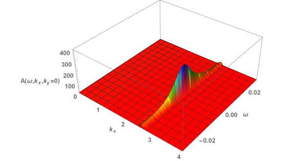
Figure 4: The spectral function $A^{0}(\omega,k_{x},k_{y}=0)$ at the critical temperature calculated numerically, showing a peak at $k_{F}=2.573$, for $q_{f}=1.7$, $\mu_{0}=2.35$, and scalar $\Delta=1$.

in the limit $\epsilon\to 0$. Using (45), the spectral function at the critical temperature $T_{c}$ and small frequencies is plotted in Fig. 4 for different values of $k_{x}$ and $k_{y}=0$. The plot shows the Fermi surface as a peak of the spectral function at $k_{x}=k_{F}=2.653$. However, the peak is quite broad indicating an instability of the quasi-particles.

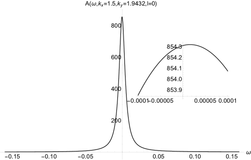
Figure 5: The spectral function $A^{0}(\omega,k_{x}=1.5,k_{y}=1.9432)$ at the critical temperature calculated numerically, showing a peak at $k_{F}=\sqrt{k_{x}^{2}+k_{y}^{2}}=2.4548$, for $q_{f}=1.7$, $\mu_{0}=2.2507$, and scalar $\Delta=1$.

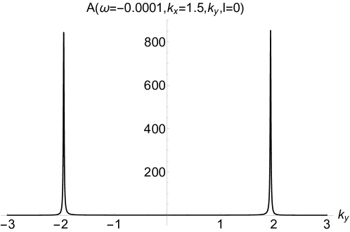
Figure 6: The spectral function $A^{0}(\omega=-0.0001,k_{x}=1.5,k_{y})$ at the critical temperature calculated numerically, showing peaks at $k_{y}=\pm 1.9432$, implying $k_{F}=\sqrt{k_{x}^{2}+k_{y}^{2}}=2.4548$, for $q_{f}=1.7$, $\mu_{0}=2.2507$, and scalar $\Delta=1$.

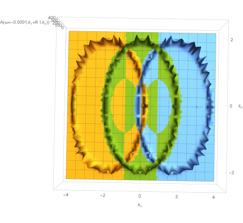
Figure 7: The spectral function $A^{l}(\omega=-0.0001,k_{x},k_{y})$ at the critical temperature calculated numerically for $l=-1,0,+1$, $q_{f}=1.56$, $\mu_{0}=2.2507$, and scalar $\Delta=1$.

Using the rotation outlined in Appendix B, we calculate numerically the spectral function at the critical temperature for non-zero values of both $k_{x}$ and $k_{y}$ and plot the results in Figures 5, 6, and 7. Figure 5 is a plot of the spectral function with $k_{x}=1.5,k_{y}=1.9432$ as a function of $\omega$ at the location of the peak along the line $k_{y}=1.9432$. There is a peak at small frequency with $k_{F}=\sqrt{k_{x}^{2}+k_{y}^{2}}=2.4548$ for parameters $q_{f}=1.7$, $\mu_{0}=2.2507$, and scalar dimension $\Delta=1$ at the critical temperature. Similarly, we plotted the spectral function as a function of $k_{y}$ in Fig. 6 for the same parameters and at small frequency ($\omega=-.0001$). The plot shows a peak at $k_{y}=\pm 1.9432$ confirming that $k_{F}=2.4548$. Finally, Fig. 7 shows the Fermi surface for $l=1,0,-1$, from left to right, respectively. We used the same parameters for plotting Fig. 7 but the fermion charge is $q_{f}=1.56$. As seen in Fig. 7 the $k_{F}$ value is smaller for a smaller $q_{F}$ value.

V Fermionic solution below the critical temperature

Having obtained the solution to the Dirac equation at the small critical temperature, we proceed to calculate the solution below the critical temperature perturbatively. For non-trivial physical results, it is necessary to include second-order effects.

V.1 First Order

Starting with the $l$-th mode at the critical temperature, at $\mathcal{O}(\xi^{2})$ below the critical temperature, three modes are excited, with $l^{\prime}=l,l\pm 1$. For an analytic solution, as in Section IV, we need to analyze the near-horizon region. After performing the rotation described in Appendix B at first order,

$$\left(\begin{array}[]{c}\tilde{\psi}_{+s}^{1,l}\\ \tilde{\psi}_{-s}^{1,l}\end{array}\right)=\left(\begin{array}[]{cc}\cos\frac{\theta}{2}&-\sin\frac{\theta}{2}\\ \sin\frac{\theta}{2}&\cos\frac{\theta}{2}\end{array}\right)\left(\begin{array}[]{c}{\psi}_{+s}^{1,l}\\ {\psi}_{-s}^{1,l}\end{array}\right)$$ (46)

where $\tan\theta=\frac{k_{y}}{k_{x}+2kl}$, and defining

$$\tilde{\psi}_{\alpha s}^{1,l}=\frac{1}{\sqrt{2}}\left(1-\frac{u^{2}}{u_{0}^{2}}\right)^{-1/4}(1+i\sigma^{1})\tilde{y}_{\alpha s}^{1,l}(u)~{}.$$ (47)

the first-order massless Dirac equation near the horizon becomes

$$\partial_{u}\tilde{y}_{\alpha s}^{1,l^{\prime}}-\frac{i}{1-\frac{u^{2}}{u_{0}^{2}}}\sigma^{3}\left(1+q_{f}A_{t}^{0}\right)\tilde{y}_{\alpha s}^{1,l^{\prime}}-\frac{\alpha\sqrt{2}k_{l}}{\mu_{0}u\sqrt{1-\frac{u^{2}}{u_{0}^{2}}}}\sigma^{1}\tilde{y}_{\alpha s}^{1,l^{\prime}}+\mathcal{A}_{\alpha s}^{l^{\prime}}=0~{},$$ (48)

where

$$\begin{split}\mathcal{A}_{\alpha s}^{l}=-&\frac{1}{2}Q_{zz}^{1,0}\partial_{u}\tilde{y}^{0,l}_{\alpha s}+\frac{i\left[\frac{q_{f}}{\sqrt{3}}\left(\frac{u_{0}}{u}-1\right)Q_{tt}^{1,0}+2q_{f}(u-u_{0})A_{t}^{1,0}\right]}{2u_{0}\left(1-\frac{u^{2}}{u_{0}^{2}}\right)}\sigma^{3}\tilde{y}^{0,l}_{\alpha s}\\ &-\alpha\frac{\left[(k_{x}+2kl)^{2}Q_{xx}^{1,0}-\left((k_{x}+2kl)^{2}-k_{l}^{2}\right)Q_{yy}^{1,0}\right]}{\sqrt{2}\mu_{0}k_{l}u\sqrt{1-\frac{u^{2}}{u_{0}^{2}}}}\sigma^{1}\tilde{y}^{0,l}_{\alpha s}\\ &-\alpha\frac{\left(k_{x}+2kl+\alpha k_{l}\right)\left(Q_{xx}^{1,0}-Q_{yy}^{1,0}\right)}{\sqrt{2}u\sqrt{1-\frac{u^{2}}{u_{0}^{2}}}k_{l}}\sigma^{1}\tilde{y}^{0,l}_{-\alpha\ 3-s}\end{split}$$ (49)

$$\begin{split}\mathcal{A}_{\alpha s}^{l\pm 1}=-&\frac{1}{4}Q_{zz}^{1,1}\partial_{u}\tilde{y}^{0,l}_{\alpha s}+\frac{i\left[\frac{q_{f}}{\sqrt{3}}\left(\frac{u_{0}}{u}-1\right)Q_{tt}^{1,1}+2q_{f}(u-u_{0})A_{t}^{1,1}\right]}{4u_{0}\left(1-\frac{u^{2}}{u_{0}^{2}}\right)}\sigma^{3}\tilde{y}^{0,l}_{\alpha s}-\alpha\frac{\pm k\left(k_{x}+2kl\right)Q_{zz}^{1,1}}{2\sqrt{2}k_{l}u}\sigma^{1}\tilde{y}^{0,l}_{\alpha s}\\ &-\frac{\alpha\left[\left(k_{l}^{2}-\left(k_{x}+2kl\right)^{2}\right)Q_{yy}^{1,1}+\left(k_{x}+2kl\right)\left(k_{x}\pm k+2kl\right)Q_{xx}^{1,1}\right]}{2\sqrt{2}\ u\sqrt{1-\frac{u^{2}}{u_{0}^{2}}}k_{l\mp 1}}\sigma^{1}\tilde{y}^{0,l}_{\alpha s}\\ &-\frac{\alpha\left(k_{x}+2kl+k_{l}\right)\left[\left(k_{x}\pm k+2kl)\right)Q_{xx}^{1,1}-(k_{x}+2kl)Q_{yy}^{1,1}\right]}{2\sqrt{2}\ u\sqrt{1-\frac{u^{2}}{u_{0}^{2}}}k_{l}}\sigma^{1}\tilde{y}^{0,l}_{-\alpha\ 3-s}\\ &\mp\frac{\alpha\left(k_{x}+2kl+k_{l}\right)kQ_{zz}^{1,1}}{2\sqrt{2}\ u\sqrt{1-\frac{u^{2}}{u_{0}^{2}}}k_{l}}\sigma^{1}\tilde{y}^{0,l}_{-\alpha\ 3-s}~{},\end{split}$$ (50)

After some straightforward algebra, we deduce the second-order equation

$$\mathbf{L}_{2}[\tilde{y}_{\alpha s}^{1,l^{\prime}}]+X_{\alpha s}^{l^{\prime}}=0~{},$$ (51)

where $\mathbf{L}_{2}[\tilde{y}]$ is defined in (39), and

$$X_{\alpha s}^{l^{\prime}}=-\frac{\sqrt{2}k_{l}}{u\sqrt{1-\frac{u^{2}}{u_{0}^{2}}}}\mathcal{A}_{\alpha s}^{l^{\prime}}+i\frac{1+q_{f}A_{t}^{0}}{1-\frac{u^{2}}{u_{0}^{2}}}\mathcal{A}_{-\alpha\ 3-s}^{l^{\prime}}+\frac{\alpha}{u\sqrt{1-\frac{u^{2}}{u_{0}^{2}}}}\partial_{u}\left(u\sqrt{1-\frac{u^{2}}{u_{0}^{2}}}\mathcal{A}_{-\alpha\ 3-s}^{l^{\prime}}\right)~{}.$$ (52)

The solution obeying the correct boundary condition at the horizon is

$$\tilde{y}_{\alpha s}^{1,l^{\prime}}(u)=-\tilde{y}_{\alpha s}^{0,l}(u)\int_{u}^{\infty}du^{\prime}\frac{\check{\tilde{y}}_{\alpha s}^{0,l}(u^{\prime})X_{\alpha s}^{l^{\prime}}(u^{\prime})}{W(u^{\prime})}+\check{\tilde{y}}_{\alpha s}^{0,l}(u)\int_{u}^{\infty}du^{\prime}\frac{\tilde{y}_{\alpha s}^{0,l}(u^{\prime})X_{\alpha s}^{l^{\prime}}(u^{\prime})}{W(u^{\prime})}~{},$$ (53)

where $\tilde{y}_{\alpha s}^{0,l}$ is the zeroth-order solution satisfying ingoing boundary conditions at the horizon (Eqs. (41) and (42)), $\check{\tilde{y}}_{\alpha s}^{0,l}$ is a linearly independent zeroth-order solution satisfying outgoing boundary conditions at the horizon, and $W$ is their Wronskian.

This first-order solution ought to be matched with the solution in the far region. Its asymptotic expression in the overlap region as a function of the frequency includes terms which behave as $\omega^{0}$, $\omega^{2\nu_{k_{l^{\prime}}}}$, and $\omega^{\nu_{k_{l^{\prime}}}\pm\nu_{k_{l}}}$, respectively. The potentially divergent terms proportional to $\omega^{\nu_{k_{l^{\prime}}}-\nu_{k_{l}}}$ do not contribute to the Green function, because they can be absorbed into the overall (physically irrelevant) normalization of the solutions to the Dirac equation.

Care must be exercised in the important special case of degeneracy ($\nu_{k_{l^{\prime}}}=\nu_{k_{l}}$), which is relevant to the calculation of the gap. The solution in this case can be found by carefully taking the limit $\nu_{k_{l^{\prime}}}\to\nu_{k_{l}}$. We obtain a solution whose asymptotic expression in the overlap region contains terms which behave as $\omega^{0}$, $\omega^{2\nu_{k_{l}}}$, and $\omega^{2\nu_{k_{l}}}\ln\omega$, respectively, all of which are well-behaved in the limit $\omega\to 0$.

We also calculated the first-order solution to the Dirac equation numerically and found good agreement with the analytic expressions. However, a calculation of the retarded Green function revealed no gap below the critical temperature. To see the pseudogap, we need to include second-order effects which we proceed to calculate next.

V.2 Second Order

At second order, i.e., at $\mathcal{O}(\xi^{4})$, below the critical temperature, five modes are excited, with $l^{\prime}=l,l\pm 1,l\pm 2$. For an analytic solution, we need to analyze the near-horizon region, as in the first-order case. After performing the rotation described in Appendix B at second order,

$$\left(\begin{array}[]{c}\tilde{\psi}_{+s}^{2,l}\\ \tilde{\psi}_{-s}^{2,l}\end{array}\right)=\left(\begin{array}[]{cc}\cos\frac{\theta}{2}&-\sin\frac{\theta}{2}\\ \sin\frac{\theta}{2}&\cos\frac{\theta}{2}\end{array}\right)\left(\begin{array}[]{c}{\psi}_{+s}^{2,l}\\ {\psi}_{-s}^{2,l}\end{array}\right)$$ (54)

where $\tan\theta=\frac{k_{y}}{k_{x}+2kl}$, and defining

$$\tilde{\psi}_{\alpha s}^{2,l}=\frac{1}{\sqrt{2}}\left(1-\frac{u^{2}}{u_{0}^{2}}\right)^{-1/4}(1+i\sigma^{1})\tilde{y}_{\alpha s}^{2,l}(u)~{}.$$ (55)

the second-order massless Dirac equation near the horizon becomes

$$\partial_{u}\tilde{y}_{\alpha s}^{2,l^{\prime}}-\frac{i}{1-\frac{u^{2}}{u_{0}^{2}}}\sigma^{3}\left(1+q_{f}A_{t}^{0}\right)\tilde{y}_{\alpha s}^{2,l^{\prime}}-\frac{\alpha\sqrt{2}k_{l}}{\mu_{0}u\sqrt{1-\frac{u^{2}}{u_{0}^{2}}}}\sigma^{1}\tilde{y}_{\alpha s}^{2,l^{\prime}}+\mathcal{B}_{\alpha s}^{l^{\prime}}=0~{},$$ (56)

where

$$\begin{split}\mathcal{B}_{\alpha s}^{l}&=\frac{3}{16}\left(2{Q_{zz}^{1,0}}^{2}+{Q_{zz}^{1,1}}^{2}\right)\partial_{u}\tilde{y}^{0,l}_{\alpha s}-\frac{1}{2}Q_{zz}^{1,0}\partial_{u}\tilde{y}^{1,l}_{\alpha s}-\frac{1}{2}Q_{zz}^{1,0}\partial_{u}\tilde{y}^{1,l}_{\alpha s}-\frac{1}{4}Q_{zz}^{1,1}\partial_{u}\tilde{y}^{1,l-1}_{\alpha s}-\frac{1}{4}Q_{zz}^{1,1}\partial_{u}\tilde{y}^{1,l+1}_{\alpha s}\\ &+\frac{iQ_{tt}^{1,0}\left[q_{f}(u-u_{0})\left(\sqrt{3}Q_{tt}^{1,0}-4uA_{t}^{1,0}\right)-3uu_{0}Q_{tt}^{1,0}\right]}{8uu_{0}\left(1-\frac{u^{2}}{u_{0}^{2}}\right)}\sigma^{3}\tilde{y}_{\alpha s}^{0,l}\\ &+\frac{iQ_{tt}^{1,1}\left[Q_{tt}^{1,1}\left(\sqrt{3}q_{f}(u-u_{0})-3uu_{0}\right)+4q_{f}u(u_{0}-u)A_{t}^{1,1}\right]}{16uu_{0}\left(1-\frac{u^{2}}{u_{0}^{2}}\right)}\sigma^{3}\tilde{y}_{\alpha s}^{0,l}\\ &+\sum_{l^{\prime}=l\pm 1}\frac{iQ_{tt}^{1,1}\left(\sqrt{3}q_{f}(u_{0}-u)+3uu_{0}\right)+6q_{f}u(u-u_{0})A_{t}^{1,1}}{12uu_{0}}\sigma^{3}\tilde{y}_{\alpha s}^{1,l^{\prime}}\\ &+\frac{iQ_{tt}^{1,0}\left(\sqrt{3}q_{f}(u_{0}-u)+3uu_{0}\right)+6q_{f}u(u-u_{0})A_{t}^{1,0}}{12uu_{0}}\sigma^{3}\tilde{y}_{\alpha s}^{1,l}\\ &-\alpha\sum_{l^{\prime}=l\pm 1}\frac{Q_{xx}^{1,1}(2kl^{\prime}+k_{x})(k(2l+1)+k_{x})-Q_{yy}^{1,1}\left((2kl^{\prime}+k_{x})^{2}-k_{l^{\prime}}^{2}\right)-kQ_{zz}^{1,1}(2kl^{\prime}+k_{x})}{2\sqrt{2\left(1-\frac{u^{2}}{u_{0}^{2}}\right)}\mu_{0}uk_{l^{\prime}}}\sigma^{1}\tilde{y}_{\alpha s}^{1,l^{\prime}}\\ &+\frac{3\alpha\left(-\left(2{Q_{yy}^{1,0}}^{2}+{Q_{yy}^{1,1}}^{2}\right)\left((2kl+k_{1})^{2}-k_{l}^{2}\right)+\left(2{Q_{xx}^{1,0}}^{2}+{Q_{xx}^{1,1}}^{2}\right)(2kl+k_{1})^{2}\right)}{8\sqrt{2\left(1-\frac{u^{2}}{u_{0}^{2}}\right)}\mu_{0}uk_{l}}\sigma^{1}\tilde{y}_{\alpha s}^{0,l}\\ &-\alpha\frac{Q_{xx}^{1,0}(2kl+k_{1})^{2}-Q_{yy}^{1,0}\left((2kl+k_{1})^{2}-k_{l}^{2}\right)}{\sqrt{2\left(1-\frac{u^{2}}{u_{0}^{2}}\right)}\mu_{0}uk_{l}}\sigma^{1}\tilde{y}_{\alpha s}^{1,l}\\ &+\alpha\frac{3(2kl+k_{1})(2kl+k_{1}+k_{l})\left(2{Q_{xx}^{1,0}}^{2}+{Q_{xx}^{1,1}}^{2}-2{Q_{yy}^{1,0}}^{2}-{Q_{yy}^{1,1}}^{2}\right)}{8\sqrt{2\left(1-\frac{u^{2}}{u_{0}^{2}}\right)}\mu_{0}uk_{l}}\sigma^{1}\tilde{y}_{-\alpha 3-s}^{0,l}\\ &-\alpha\frac{(2kl+k_{1})(Q_{xx}^{1,0}-Q_{yy}^{1,0})(2kl+k_{x}+k_{l})}{\sqrt{2\left(1-\frac{u^{2}}{u_{0}^{2}}\right)}\mu_{0}uk_{l}}\sigma^{1}\tilde{y}_{-\alpha 3-s}^{1,l}\\ &-\alpha\sum_{l^{\prime}=l\pm 1}\frac{((2kl^{\prime}+k_{1}\mp k)Q_{xx}^{1,1}-(2kl^{\prime}+k_{1})Q_{yy}^{1,1}\pm kQ_{zz}^{1,1})(2kl^{\prime}+k_{x}+k_{l}^{\prime})}{2\sqrt{2\left(1-\frac{u^{2}}{u_{0}^{2}}\right)}\mu_{0}uk_{l}^{\prime}}\sigma^{1}\tilde{y}_{-\alpha 3-s}^{1,l^{\prime}}\end{split}$$ (57)

$$\begin{split}\mathcal{B}_{\alpha s}^{l\pm 1}&=\frac{3}{8}Q_{zz}^{1,0}Q_{zz}^{1,1}\partial_{u}\tilde{y}^{0,l}_{\alpha s}-\frac{Q_{zz}^{1,1}}{4}\partial_{u}\tilde{y}^{1,l}_{\alpha s}-\frac{Q_{zz}^{1,1}}{2}\partial_{u}\tilde{y}^{1,l+1}_{\alpha s}\\ &+\frac{i\left(Q_{tt}^{1,0}\left(Q_{tt}^{1,1}\left(\sqrt{3}q_{f}(u-u_{0})-3uu_{0}\right)+2q_{f}u(u_{0}-u)A_{t}^{1,1}\right)+2q_{f}uQ_{tt}^{1,1}(u_{0}-u)A_{t}^{1,0}\right)}{8uu_{0}\left(1-\frac{u^{2}}{u_{0}^{2}}\right)}\sigma^{3}\tilde{y}^{0,l}_{\alpha s}\\ &+\frac{i\left(Q_{tt}^{1,1}\left(\sqrt{3}q_{f}(u_{0}-u)+3uu_{0}\right)+6q_{f}u(u-u_{0})A_{t}^{1,1}\right)}{12uu_{0}\left(1-\frac{u^{2}}{u_{0}^{2}}\right)}\sigma^{3}\tilde{y}^{1,l}_{\alpha s}\\ &+\frac{i\left(Q_{tt}^{1,0}\left(\sqrt{3}q_{f}(u_{0}-u)+3uu_{0}\right)+6q_{f}u(u-u_{0})A_{t}^{1,0}\right)}{6uu_{0}\left(1-\frac{u^{2}}{u_{0}^{2}}\right)}\sigma^{3}\tilde{y}^{1,l+1}_{\alpha s}\\ &+\alpha\frac{Q_{xx}^{1,0}(2kl+k_{x})(3Q_{xx}^{1,1}(\mp k+2kl+k_{x})+kQ_{zz}^{1,1})}{4\sqrt{2\left(1-\frac{u^{2}}{u_{0}^{2}}\right)}\mu_{0}uk_{l}}\sigma^{1}\tilde{y}^{0,l}_{\alpha s}\\ &-\alpha\frac{3Q_{yy}^{1,0}Q_{yy}^{1,1}\left((2kl+k_{x})^{2}-k_{l}^{2}\right)-2kQ_{zz}^{1,0}Q_{zz}^{1,1}(2kl+k_{x})}{4\sqrt{2\left(1-\frac{u^{2}}{u_{0}^{2}}\right)}\mu_{0}uk_{l}}\sigma^{1}\tilde{y}^{0,l}_{\alpha s}\\ &+\alpha\frac{Q_{xx}^{1,1}(-(2kl+k_{x}))(\mp k+2kl+k_{x})-kQ_{zz}^{1,1}(2kl+k_{x})+Q_{yy}^{11}\left((2kl+k_{x})^{2}-k_{l}^{2}\right)}{2\sqrt{2\left(1-\frac{u^{2}}{u_{0}^{2}}\right)}\mu_{0}uk_{l\pm 1}}\sigma^{1}\tilde{y}^{1,l}_{\alpha s}\\ &-\alpha\frac{(k_{x}+2(k\pm 1))^{2}Q_{xx}^{1,0}+\left((2k(l\pm 1)+k_{1})^{2}-k_{l\pm 1}^{2}\right)Q_{yy}^{1,0}}{\sqrt{2\left(1-\frac{u^{2}}{u_{0}^{2}}\right)}\mu_{0}uk_{l\pm 1}}\sigma^{1}\tilde{y}^{1,l\pm 1}_{\alpha s}\\ &+\alpha\frac{Q_{xx}^{1,0}((2kl+k_{x}+k_{l})(3Q_{xx}^{1,1}(2kl\pm k+k_{1})+kQ_{zz}^{1,1})}{4\sqrt{2\left(1-\frac{u^{2}}{u_{0}^{2}}\right)}\mu_{0}uk_{l\pm 1}}\sigma^{1}\tilde{y}^{0,l}_{-\alpha 3-s}\\ &-\alpha\frac{((2kl+k_{1}+k_{l})(\pm 3Q_{yy}^{1,0}Q_{yy}^{1,1}(2kl+k_{x})\mp 2kQ_{zz}^{1,0}Q_{zz}^{1,1})}{4\sqrt{2\left(1-\frac{u^{2}}{u_{0}^{2}}\right)}\mu_{0}uk_{l\pm 1}}\sigma^{1}\tilde{y}^{0,l}_{-\alpha 3-s}\\ &-\alpha\frac{(2kl+k_{x}+k_{l})((2kl+k+k_{x})Q_{xx}^{1,1}-(k_{x}+2kl)Q_{yy}^{1,1}-kQ_{zz}^{1,1})}{2\sqrt{2\left(1-\frac{u^{2}}{u_{0}^{2}}\right)}\mu_{0}uk_{l\pm 1}}\sigma^{1}\tilde{y}^{1,l}_{-\alpha 3-s}\\ &-\alpha\frac{(2k(l\pm 1)+k_{x})(2k(l\pm 1)+k_{l\pm 1}+k_{x})(Q_{xx}^{1,0}-Q_{yy}^{1,0})}{\sqrt{2\left(1-\frac{u^{2}}{u_{0}^{2}}\right)}\mu_{0}uk_{l\pm 1}}\sigma^{1}\tilde{y}^{1,l\pm 1}_{-\alpha 3-s}\end{split}$$ (58)

$$\begin{split}\mathcal{B}_{\alpha s}^{l\pm 2}&=-\frac{1}{4}Q_{zz}^{1,1}\partial_{u}\tilde{y}^{1,l\pm 1}_{\alpha s}+\frac{i\left(Q_{tt}^{1,1}\left(\sqrt{3}q_{f}(u_{0}-u)+3uu_{0}\right)+6q_{f}u(u-u_{0})A_{t}^{1,1}\right)}{12uu_{0}\left(1-\frac{u^{2}}{u_{0}^{2}}\right)}\tilde{y}^{1,l\pm 1}_{\alpha s}\\ &+\alpha\frac{Q_{yy}^{1,1}\left((2k(l\pm 1)+k_{x})^{2}-k_{l\pm 1}^{2}\right)+Q_{xx}^{1,1}(-(2k(l\pm 1)+k_{x}))(k(2l-3)+k_{x})}{2\sqrt{2\left(1-\frac{u^{2}}{u_{0}^{2}}\right)}\mu_{0}uk_{l\pm 1}}\sigma^{1}\tilde{y}^{1,l\pm 1}_{\alpha s}\\ &-\alpha\frac{kQ_{zz}^{1,1}(2k(l\pm 1)+k_{x})}{2\sqrt{2\left(1-\frac{u^{2}}{u_{0}^{2}}\right)}\mu_{0}uk_{l\pm 1}}\sigma^{1}\tilde{y}^{1,l\pm 1}_{\alpha s}\\ &-\frac{(2k(l\pm 1)+k_{x}+k_{l\pm 1})(Q_{xx}^{1,1}(k(2l-3)+k_{x})-Q_{yy}^{1,1}(2k(l\pm 1)+k_{x})+kQ_{zz}^{1,1})}{2\sqrt{2\left(1-\frac{u^{2}}{u_{0}^{2}}\right)}\mu_{0}uk_{l\pm 1}}\sigma^{1}\tilde{y}^{1,l\pm 1}_{-\alpha\ 3-s}\end{split}$$ (59)

After some algebra, we arrive at the second order equation

$$\mathbf{L}_{2}[\tilde{y}_{\alpha s}^{2,l^{\prime}}]+Y_{\alpha s}^{l^{\prime}}=0~{},$$ (60)

where $\mathbf{L}_{2}[\tilde{y}]$ is defined in (39), and

$$Y_{\alpha s}^{l^{\prime}}=-\frac{\sqrt{2}k_{l}}{u\sqrt{1-\frac{u^{2}}{u_{0}^{2}}}}\mathcal{B}_{\alpha s}^{l^{\prime}}+i\frac{1+q_{f}A_{t}^{0}}{1-\frac{u^{2}}{u_{0}^{2}}}\mathcal{B}_{-\alpha\ 3-s}^{l^{\prime}}+\frac{\alpha}{u\sqrt{1-\frac{u^{2}}{u_{0}^{2}}}}\partial_{u}\left(u\sqrt{1-\frac{u^{2}}{u_{0}^{2}}}\mathcal{B}_{-\alpha\ 3-s}^{l^{\prime}}\right)~{}.$$ (61)

The solution obeying the correct boundary condition at the horizon is (cf. with its first-order counterpart (53))

$$\tilde{y}_{\alpha s}^{2,l^{\prime}}(u)=-\tilde{y}_{\alpha s}^{0,l}(u)\int_{u}^{\infty}du^{\prime}\frac{\check{\tilde{y}}_{\alpha s}^{0,l}(u^{\prime})Y_{\alpha s}^{l^{\prime}}(u^{\prime})}{W(u^{\prime})}+\check{\tilde{y}}_{\alpha s}^{0,l}(u)\int_{u}^{\infty}du^{\prime}\frac{\tilde{y}_{\alpha s}^{0,l}(u^{\prime})Y_{\alpha s}^{l^{\prime}}(u^{\prime})}{W(u^{\prime})}~{}.$$ (62)

As before, this second-order solution ought to be matched with the solution in the far region. Its asymptotic expression in the overlap region as a function of the frequency includes terms which behave as $\omega^{0}$, $\omega^{2\nu_{k_{l^{\prime}}}}$, and $\omega^{\nu_{k_{l^{\prime}}}\pm\nu_{k_{l}}}$, respectively. The potentially divergent terms, $\omega^{\nu_{k_{l^{\prime}}}-\nu_{k_{l}}}$, may be absorbed into the overall normalization of the solutions, as in first order.

In the special case of degeneracy ($\nu_{k_{l^{\prime}}}=\nu_{k_{l}}$), which contributes to the gap at second order, the solution can be found by carefully taking the limit $\nu_{k_{l^{\prime}}}\to\nu_{k_{l}}$. We obtain a solution whose asymptotic expression in the overlap region contains terms which behave as $\omega^{0}$, $\ln\omega$, $\omega^{2\nu_{k_{l}}}$, $\omega^{2\nu_{k_{l}}}\ln\omega$, and $\omega^{2\nu_{k_{l}}}(\ln\omega)^{2}$, respectively. The terms proportional to $\ln\omega$ diverge in the limit $\omega\to 0$, however an explicit calculation shows that they do not contribute to the pole at the Fermi surface ($k_{l}=k_{F}$).

We calculated the second-order solution numerically and found good agreement with the analytic expressions. A calculation of the retarded Green function revealed no gap in the general case. However, a pseudogap emerged in the degenerate case, as we discuss next.

V.3 Generation of a gap in the Fermi surface

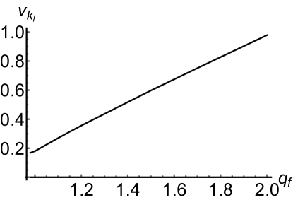
Figure 8: Plot of scaling parameter, $\nu_{k_{l}}$, as a function of fermion charge, $q_{f}$, at $k_{l}=k_{F}$ for parameters $\frac{\eta}{\mu_{0}^{2}}=0.25$, $\frac{\eta^{\prime}}{\mu_{0}^{4}}=0.005$, $q=0$, $\Delta=1$, $\mu_{0}=2.2507$, $\frac{T}{\mu_{0}}=0.0613$, and tiny frequecy $\omega=0.0001$ respectively.

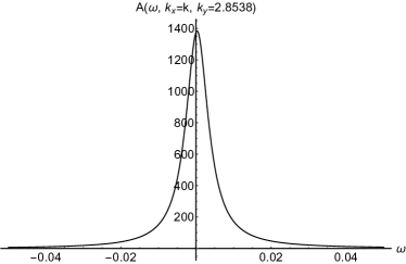
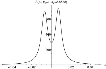
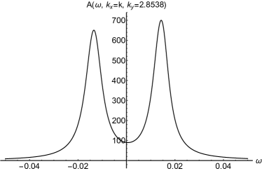
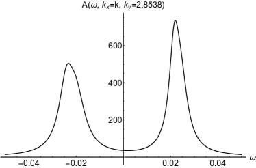
Figure 9: Plot of spectral function $A(\omega,k_{x}=k,k_{y}=2.8538)$ vs. $\omega$ for parameters $\frac{\eta}{\mu_{0}^{2}}=0.25$, $\frac{\eta^{\prime}}{\mu_{0}^{4}}=0.005$, $q=0$, $\Delta=1$, $q_{f}=2$, $\mu_{0}=2.2507$, $\frac{T}{\mu_{0}}=0.0613$ and for $\xi=0.0,0.05,0.07,0.1$ respectively.

As already discussed, the retarded Green function does not develop any pole at the Fermi surface using the general first and second order solutions of the Dirac equation. However, in the degenerate case, $\nu_{k_{l^{\prime}}}=\nu_{k_{l}}$ of the second order solution, a gap is generated in the Fermi surface corresponding to a pole in the Green function where $k_{l}=k_{F}$.

Near the Fermi surface, we can write the Green function as in LSSZ:2012 ,

$$\left(G_{R}\right)_{\alpha l,\alpha l}=\frac{A_{\alpha l,\alpha l}^{(0)}B_{\alpha l,\alpha l}^{(0)}}{(A_{\alpha l,\alpha l}^{(0)}+\xi^{4}A_{\alpha l,\alpha l}^{(2)})^{2}-\xi^{4}A_{\alpha l,\alpha l-1}^{(1)}A_{\alpha l-1,\alpha l}^{(1)}+\mathcal{O}(\xi^{6})}~{},$$ (63)

where $A^{(n)}_{\alpha l,\alpha l}$ and $B^{(n)}_{\alpha l,\alpha l}$ are the results of matching at $n$-th order in the boundary behavior (29). To find a numerical solution to the Green function (63), we solve the second order Dirac equation with ingoing boundary conditions at the horizon and plot the spectral function as a function of $\omega$ and $k_{y}$ respectively. The results of our calculations are depicted in Fig. 9 - Fig. 11 and discussed in details in the following.

Near the Fermi surface, the retarded Green functions take the general form

$$G_{R}=\frac{Z}{\omega-v_{F}(k-k_{F})+\Sigma(\omega,k)}~{},$$ (64)

where $\Sigma$ is the self energy for fermionic excitations near the Fermi surface and $Z$ is the residue of the pole and quasiparticle weight. Therefore, we can write

$$A_{\alpha l,\alpha l}^{(0)}+\xi^{4}A_{\alpha l,\alpha l}^{(2)}=\omega-v_{F}(k_{l}-k_{F})+i(c_{1}-ic_{2})\omega^{2\nu_{k_{l}}}$$ (65)

where $v_{F},c_{1},c_{2}$ are real constants determined from the boundary data.

We can distinguish three different cases for the retarded Green function depending on the value of $\nu_{k_{l}}$ Faulkner:2009wj . The $\nu_{k_{l}}$ values are plotted as a function of $q_{f}$ in Fig. 8.

• For $\nu_{k_{l}}>\frac{1}{2}$, the system has fermionic quasiparticles and the effective theory is a Fermi liquid. In this case the imaginary part of the self-energy is proportional to $\omega^{2}$. Also, the spectral function has a Lorentzian distribution centered around $\omega=0$. The dominant linear term leads the dispersion and we obtain

  $$G_{R\alpha l,\alpha l}^{-1}\sim(\omega-v_{F}(k_{l}-k_{F}))^{2}-\Delta^{2}+ic_{1}(\omega-v_{F}(k_{l}-k_{F}))\omega^{2\nu_{k_{l}}}~{}.$$ (66)

  Near the Fermi surface and with small $\omega$, there are two peaks in the spectral function, $A(\omega,k_{x},k_{y})=\Im[G_{R1l,1l}+G_{R2l,2l}]$. The peaks are found at $\omega=v_{F}(k_{l}-k_{F})\pm\Delta$ as seen in Fig. 9, and the pseudogap $\Delta$ is first order in $\xi^{2}$, given by

  $$\Delta^{2}=\xi^{4}A_{\alpha l,\alpha l-1}^{(1)}A_{\alpha l-1,\alpha l}^{(1)}~{}.$$ (67)

  The width is controlled by second-order terms. Fig. 9 also shows that the size of the gap is on the order of $\xi^{2}$, as $\omega\sim\Delta\sim\xi^{2}$. Also apparent is the pseudogap behavior as the spectral function remains non-zero over all energies. The value $\xi=0$ corresponds to temperatures above critical temperature. As we increase $\xi$, the magnitude of the gap increases but at large enough $\xi$, the perturbation breaks down. The widths are on the order of $\xi^{2\nu_{k_{l}}}$, therefore, they appear as sharp peaks. For the parameters used in plotting Fig. 9, the system is in the Fermi liquid state with $\nu_{k_{l}}=0.9787$.

  

  

  

  

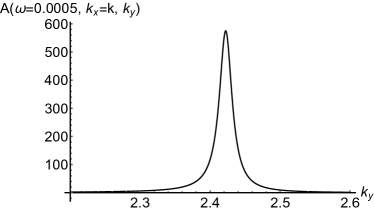
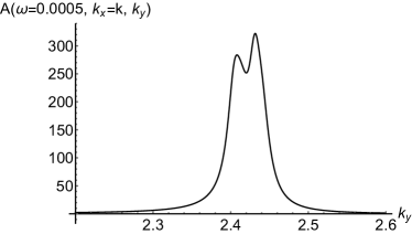
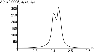
  Figure 10: Plot of spectral function $A(\omega=0.0005,k_{x}=k,k_{y})$ vs. $k_{y}$ for parameters $\frac{\eta}{\mu_{0}^{2}}=0.25$, $\frac{\eta^{\prime}}{\mu_{0}^{4}}=0.005$, $q=0$, $\Delta=1$, $q_{f}=1.8$, $\mu_{0}=2.2507$, $\frac{T}{\mu_{0}}=0.0613$ and for $\xi=0.0,0.07,0.075$ respectively.

  We also observe the presence of the pseudogap in the $A(\omega,k_{x},k_{y})$ vs. $k_{y}$ graph in Fig. 10 for different values of $\xi$. As seen from the graphs, the perturbation breaks down near $\xi\sim 0.08$.

• For $\nu_{k_{l}}<\frac{1}{2}$ in the non-Fermi liquid case, the non-analytic term dominates non-linear dispersion and we can write $A_{\alpha l,\alpha l}^{(0)}+\xi^{4}A_{\alpha l,\alpha l}^{(2)}=c_{2}\omega^{2\nu_{k_{l}}}-v_{F}(k_{l}-k_{F})+ic_{1}-\omega^{2\nu_{k_{l}}}$. This produces the Green function

  $$G_{R\alpha l,\alpha l}^{-1}\sim(\omega^{2\nu_{k_{l}}}-v_{F}(k_{l}-k_{F}))^{2}-\Delta^{2}+ic_{1}(\omega^{2\nu_{k_{l}}}-v_{F}(k_{l}-k_{F}))\omega^{2\nu_{k_{l}}}~{},$$ (68)

  and the two peaks are at $\omega^{2\nu_{k_{l}}}=v_{F}(k_{l}-k_{F})\pm\Delta$. This qualitatively differs from that of the Fermi liquid case. For the non-Fermi liquid case, the width of the non-linear dispersion and gap are on the order of $\xi^{1/2\nu_{k_{l}}}$.

  

  

  

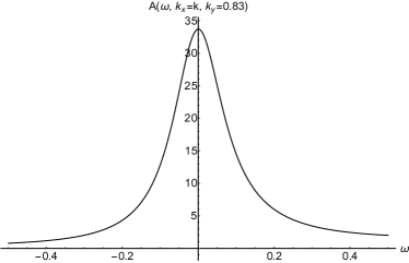
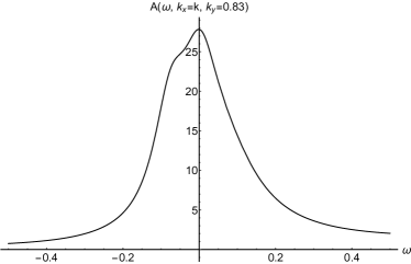
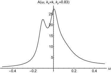
  Figure 11: Plot of spectral function, $A(\omega,k_{x}=k,k_{y}=0.83)$, as a function of $\omega$ for non-Fermi liquid case, $\nu_{k_{l}}<1/2$, with parameters $\frac{\eta}{\mu_{0}^{2}}=0.25$, $\frac{\eta^{\prime}}{\mu_{0}^{4}}=0.005$, $q=0$, $\Delta=1$, $q_{f}=1.15$, $\mu_{0}=2.2507$, $\frac{T}{\mu_{0}}=0.0613$ and for $\xi=0.0,0.25,0.3$ respectively.

  In Fig. 11 we plotted the spectral function for $\nu_{k_{l}}=0.3134<1/2$ with the parameters $\frac{\eta}{\mu_{0}^{2}}=0.25$, $\frac{\eta^{\prime}}{\mu_{0}^{4}}=0.005$, $q=0$, $\Delta=1$, $q_{f}=1.15$, $\mu_{0}=2.2507$, $\frac{T}{\mu_{0}}=0.0613$ for $\xi=0.0,0.25,0.3$. We were unable to observe a gap unless $\xi\gtrsim 0.25$. This is because the spectral functions are wide enough to hide the peaks for small values of $\xi$. Also as seen from Fig. 11, the broad peaks correspond to a lack of stable quasiparticles.

• Finally, for $\nu_{k_{l}}=\frac{1}{2}$, the system is in the marginal Fermi liquid state. There is still a Fermi surface but the self energy scaling is not quadratic in $\omega$ as $\Im\Sigma\propto\omega\ln\omega$. Therefore, near Fermi surface and small $\omega$, the $\omega$-dependence of the matrix elements of $A$ are $A_{\alpha l,\alpha l}=\omega+c_{2}\omega\ln\omega-v_{F}(k_{l}-k_{F})+ic_{1}\omega\ln\omega$.

VI Conclusion

We have studied the behavior and properties of a holographic Fermi liquid system in a spontaneously generated lattice. The Dirac field was calculated in the presence of a finite but small-temperature black hole. Exploring the holographic fermionic spectral function, we found a pseudogap at the edge of the Brillouin zone for the degenerate case, $\nu_{k_{l}}=\nu_{k_{l^{\prime}}}$, due to interactions between different levels. The magnitude of the gap increases with increasing order parameter $\xi$. However, with large enough $\xi$, the perturbation limit breaks down.

These results are consistent with the lattice effects on the Fermi surface due to a periodic potential previously studied in LSSZ:2012 and with backreaction in Ling:2013fl . However, our motivation was unique. Instead of choosing a modulated scalar potential for the electromagnetic field at the start, we introduced a higher-derivative interaction between a $U(1)$ gauge field and a scalar field. We used perturbation theory to expand the bulk fields below $T_{c}$, thus obtaining an analytic solution to the coupled system of Einstein-Maxwell-scalar field equations at first order. We found a spatially inhomogeneous charge density spontaneously generated in the boundary theory Alsup:2013kda .

We provided analytic and numerical solutions of the gap behavior in the presence of a spontaneously generated lattice. The behavior of the holographic fermionic system was studied by solving the Dirac equation in the gravitational background of the backreacted Einstein-Maxwell-scalar system. It will be interesting to perform a future study of the backreaction of Dirac fields. As it is well known, fermions should not be treated as elementary fields but as a fluid. Therefore the energy-momentum tensor of a perfect fluid must be introduced into the field equations, leading to an electron star Hartnoll:2010gu ; Allais:2013lha ; Cubrovic:2010bf with lattice effects.

Another direction of future research is to introduce a dipole coupling of fermions to an electromagnetic field Edalati:2010ww ; Guarrera:2011my ; Edalati:2010ge . There have been some studies in this direction introducing a Q-lattice background Ling:2014bda ; Ling:2015mott . It will be interesting to extend these to a fully dynamical generation of a Mott gap, and analyze the dynamically generated lattice effects as a function of the dipole coupling.

Appendix A First-order field modes

In this appendix, we calculate the metric function and Maxwell field modes at first order. Solving the Maxwell equations (6) at first order, we obtain

$$A_{t}^{1,0}(z)=C+\mathbf{a}_{t}^{1,0}(z)\ ,\ \ \mathbf{a}_{t}^{1,0}(z)=\frac{\mu_{0}}{4}\int_{1}^{z}\frac{dw}{(1-w)^{2}}\int_{1}^{w}dw^{\prime}\ {w^{\prime}}^{2\Delta-2}\frac{(1-w^{\prime})^{3}}{h^{2}(w^{\prime})}\mathcal{A}(w^{\prime})$$ (69)

where

$$\begin{split}\mathcal{A}(z)=&\left[\frac{4q^{2}(1-z)}{h(z)}\left(1+\frac{\mu_{0}^{2}z^{3}(1-z)}{4h(z)}\right)+z\left[\Delta^{2}+8k^{2}z^{2}\eta(1+\Delta)\right]\right]F^{2}(z)\\ &+z^{2}\left[2(\Delta+4k^{2}\eta z^{2})F(z)+zF^{\prime}(z)\right]F^{\prime}(z)~{}.\end{split}$$ (70)

and the integration constant $C$ remains to be determined.

Having obtained $A_{t}^{1,0}(z)$, we proceed to solve the Einstein equations to find $Q_{tt}^{1,0},Q_{zz}^{1,0},Q_{xx}^{1,0},Q_{yy}^{1,0}$. We find that $Q_{xz}^{1,0}$ does not appear in the first-order equations and can set $Q_{xz}^{1,0}(z)=0$, as a gauge choice. We find the following analytic solutions of the metric functions

$$\begin{split}Q_{tt}^{1,0}(z)=&\frac{1}{2}\mathcal{Q}_{1}(1)\left(3-\frac{\mu_{0}^{2}}{4}\right)\frac{z^{3}(1-z)}{h(z)}+\frac{z^{3}}{h(z)}\int_{1}^{z}dw\left[\frac{12\mathcal{Q}_{1}(w)}{w^{4}}\right.+\left.\frac{w^{2\Delta-4}}{4h^{2}(w)}\mathcal{Q}_{2}(w)\right]\\ &-\frac{z^{4}}{h(z)}\int_{1}^{z}dw\left[\frac{12\mathcal{Q}_{1}(w)}{w^{5}}\right.+\left.\frac{w^{2\Delta-5}}{4h^{2}(w)}\mathcal{Q}_{2}(w)\right]~{},\end{split}$$ (71)

where

$$\mathcal{Q}_{1}(z)=-\frac{1}{2}\int_{0}^{z}dw\,w^{2\Delta+1}\left(\frac{q^{2}\mu_{0}^{2}(1-w)^{2}F(w)^{2}}{h^{2}(w)}+\frac{\left(wF^{\prime}(w)+\Delta F(w)\right)^{2}}{w^{2}}\right)~{},$$ (72)

and

$$\begin{split}\mathcal{Q}_{2}(z)=&zh^{2}(z)\left(-zh^{\prime}(z)+4h(z)\right)(2\Delta F(z)+zF^{\prime}(z))F^{\prime}(z)\\ &+\left[-h^{2}(z)\left(2\left(2(\Delta-3)\Delta+k^{2}z^{2}\left(1+\eta\mu_{0}^{2}z^{4}\right)\right)+\Delta^{2}(zh^{\prime}(z)-4h(z))\right)\right.\\ &\left.\ \ \ \ \ -\mu_{0}^{2}q^{2}z^{2}(1-z)^{2}(zh^{\prime}(z)-8h(z))\right]F^{2}(z)~{}.\end{split}$$ (73)

Similarly, we find

$$Q_{zz}^{1,0}(z)=\frac{1}{2}\mathcal{Q}_{1}(1)\left(3-\frac{\mu_{0}^{2}}{4}\right)\frac{z^{3}(1-z)}{h(z)}+\frac{z^{3}}{4h(z)}\int_{1}^{z}dw\frac{w^{2\Delta-5}(w-z)}{h^{2}(w)}\mathcal{Q}_{3}(w)~{},$$ (74)

where

$$\begin{split}\mathcal{Q}_{3}(z)=&2zh\left(3\Delta zhh^{\prime}+2\Delta(3\Delta-4)h^{2}+2q^{2}\mu_{0}^{2}(1-z)^{2}z^{2}\right)F^{\prime}F\\ &+\left[h^{2}\left(3\Delta^{2}zh^{\prime}-2\left(2(\Delta-3)\Delta+k^{2}z^{2}\left(1+\eta\mu_{0}^{2}z^{4}\right)\right)\right)-q^{2}\mu_{0}^{2}(1-z)^{2}z^{3}h^{\prime}\right]F^{2}\\ &+\left[2q^{2}\mu_{0}^{2}(1-z)z^{2}h(2\Delta(1-z)-1-z)+2\Delta^{2}(2\Delta-5)h^{3}\right]F^{2}\\ &+4\Delta z^{2}h^{3}F^{\prime\prime}\left[\Delta F+zF^{\prime}\right]+\left[z^{2}h^{2}\left(3zh^{\prime}+(8\Delta-6)h\right)\right]{F^{\prime}}^{2}~{}.\end{split}$$ (75)

The remaining modes are found to be

$$Q_{xx}^{1,0}(z)=-\frac{1}{2}k^{2}\int_{0}^{z}dw\frac{w^{2}}{h(w)}\int_{1}^{w}dw^{\prime}{w^{\prime}}^{2\Delta-2}(1-\eta\mu_{0}^{2}{w^{\prime}}^{4})F^{2}(w^{\prime})~{},$$ (76)

and, lastly,

$$Q_{yy}^{1,0}(z)=-Q_{xx}^{1,0}(z)~{}.$$ (77)

Having obtained $A_{t}^{1,0}$ and $Q_{\mu\nu}^{1,0}$, the $Q_{\mu\nu}^{1,1}$ and $A_{t}^{1,1}$ modes may be deduced from the remaining Einstein-Maxwell equations. These amount to six equations with six unknown functions. Two of the equations are first order. The system of equations to be solved numerically is comprised of

$$\begin{split}&{Q_{xx}^{1,1}}^{\prime\prime}+{Q_{yy}^{1,1}}^{\prime\prime}-\frac{z\left(8k^{2}z-4h^{\prime}+\mu_{0}^{2}z^{3}\right)+12h}{2z^{2}h}Q_{zz}^{1,1}-\frac{4k^{2}}{h}Q_{yy}^{1,1}\\ &-\frac{2kz^{2}h^{\prime}}{h}Q_{xz}^{1,1}-4kz^{2}{Q_{xz}^{1,1}}^{\prime}+\frac{2}{z}{Q_{zz}^{1,1}}^{\prime}+\frac{zh^{\prime}-4h}{2zh}\left({Q_{xx}^{1,1}}+{Q_{yy}^{1,1}}\right)^{\prime}-\frac{\mu_{0}^{2}z^{2}}{2h}Q_{tt}^{1,1}\\ &-\frac{\mu_{0}z^{2}(1-z)}{h}{A_{t}^{1,1}}^{\prime}+\frac{\mu_{0}z^{2}}{h}A_{t}^{1,1}+z^{2\Delta-2}\mathcal{Q}_{4}=0~{},\end{split}$$ (78)

$$\begin{split}&(-zh^{\prime}+4h)\left(Q_{xx}^{1,1}+Q_{yy}^{1,1}\right)^{\prime}+4h{Q_{tt}^{1,1}}^{\prime}+\left(-4h^{\prime}+\mu_{0}^{2}z^{3}+\frac{12h}{z}\right)Q_{zz}^{1,1}\\ &-4kz^{2}(-zh^{\prime}+4h)Q_{xz}^{1,1}(z)+\left(8k^{2}z+\mu_{0}^{2}z^{3}\right)Q_{tt}^{1,1}+8k^{2}zQ_{yy}^{1,1}\\ &-2\mu_{0}z^{3}A_{t}^{1,1}+2\mu_{0}(1-z)z^{3}{A_{t}^{1,1}}^{\prime}+2z^{2\Delta-1}h\mathcal{Q}_{5}=0~{},\end{split}$$ (79)

$$\begin{split}{Q_{tt}^{1,1}}^{\prime}+{Q_{yy}^{1,1}}^{\prime}+\frac{h^{\prime}}{2h}Q_{tt}^{1,1}+\frac{4h-zh^{\prime}}{2zh}Q_{zz}^{1,1}+\frac{\mu_{0}z^{2}(1-z)}{h}A_{t}^{1,1}+z^{2\Delta-1}\mathcal{Q}_{6}=0~{},\end{split}$$ (80)

$$\begin{split}&{Q_{tt}^{1,1}}^{\prime\prime}+{Q_{yy}^{1,1}}^{\prime\prime}+\frac{-3zh^{\prime}+4h}{2zh}{Q_{tt}^{1,1}}^{\prime}+\frac{zh^{\prime}-2h}{zh}{Q_{yy}^{1,1}}^{\prime}-\frac{zh^{\prime}-4h}{2zh}{Q_{zz}^{1,1}}^{\prime}+\frac{\mu_{0}^{2}z^{2}}{2h}Q_{tt}^{1,1}\\ &+\frac{\mu_{0}z^{2}(1-z)}{h}{A_{t}^{1,1}}^{\prime}-\frac{z\left(8h^{\prime}+2zh^{\prime\prime}-\mu_{0}^{2}z^{3}\right)+12h}{2z^{2}h}Q_{zz}^{1,1}-\frac{\mu_{0}z^{2}}{h}A_{t}^{1,1}+z^{2\Delta-2}\mathcal{Q}_{7}=0~{},\end{split}$$ (81)

$$\begin{split}&{Q_{tt}^{1,1}}^{\prime\prime}+{Q_{xx}^{1,1}}^{\prime\prime}-\frac{z\left(8k^{2}z-8h^{\prime}+2zh^{\prime\prime}-\mu_{0}^{2}z^{3}\right)+12h}{2z^{2}h}Q_{zz}^{1,1}\\ &-\frac{8k^{2}-\mu_{0}^{2}z^{2}}{2h}Q_{tt}^{1,1}-\frac{4kz^{2}h^{\prime}}{h}Q_{xz}^{1,1}+\frac{3zh^{\prime}-4h}{zh}{Q_{tt}^{1,1}}^{\prime}+\frac{zh^{\prime}-2h}{zh}{Q_{xx}^{1,1}}^{\prime}-\frac{zh^{\prime}-4h}{2zh}{Q_{zz}^{1,1}}^{\prime}\\ &+\frac{\mu_{0}z^{2}(1-z)}{h}{A_{t}^{1,1}}^{\prime}-\frac{\mu_{0}z^{2}}{h}A_{t}^{1,1}-4kz^{2}{Q_{xz}^{1,1}}^{\prime}+z^{2\Delta-2}\mathcal{Q}_{8}=0~{},\end{split}$$ (82)

and

$$\begin{split}&{A_{t}^{1,1}}^{\prime\prime}-\frac{4k^{2}}{h}A_{t}^{1,1}-\frac{2}{1-z}{A_{t}^{1,1}}^{\prime}+\frac{2k\mu_{0}z^{2}}{1-z}Q_{xz}^{1,1}\\ &+\frac{\mu_{0}}{2(1-z)}({Q_{tt}^{1,1}}-{Q_{xx}^{1,1}}-{Q_{yy}^{1,1}}+{Q_{zz}^{1,1}})^{\prime}-\frac{\mu_{0}z^{2\Delta-2}\left(q^{2}-2\eta k^{2}z^{3}h\right)}{(1-z)h}F^{2}=0~{},\end{split}$$ (83)

where

$$\mathcal{Q}_{4}=\frac{1}{2}z^{2}F^{\prime 2}+\Delta zFF^{\prime}+\frac{\left((\Delta-3)\Delta-k^{2}z^{2}\left(1+\eta\mu_{0}^{2}z^{4}\right)\right)h+\Delta^{2}h^{2}+\mu_{0}^{2}q^{2}(1-z)^{2}z^{2}}{2h^{2}}F^{2}~{},$$

$$\mathcal{Q}_{5}=\frac{1}{2}z^{2}F^{\prime 2}+\Delta zFF^{\prime}+\frac{\left(-(\Delta-3)\Delta+k^{2}z^{2}\left(1+\eta\mu_{0}^{2}z^{4}\right)\right)h+\Delta^{2}h^{2}+\mu_{0}^{2}q^{2}(1-z)^{2}z^{2}}{2h^{2}}F^{2}~{},$$

$$\begin{split}\mathcal{Q}_{6}=&\frac{1}{2}F\left(zF^{\prime}+\Delta F\right)~{},\end{split}$$

$$\mathcal{Q}_{7}=\frac{1}{2}z^{2}F^{\prime 2}+\Delta zFF^{\prime}+\frac{\left((\Delta-3)\Delta+k^{2}z^{2}\left(1-\eta\mu_{0}^{2}z^{4}\right)\right)h+\Delta^{2}h^{2}-\mu_{0}^{2}q^{2}(1-z)^{2}z^{2}}{2h^{2}}F^{2}~{},$$

$$\mathcal{Q}_{8}=\frac{1}{2}z^{2}F^{\prime 2}+\Delta zFF^{\prime}+\frac{\left((\Delta-3)\Delta-k^{2}z^{2}\left(1-\eta\mu_{0}^{2}z^{4}\right)\right)h+\Delta^{2}h^{2}-\mu_{0}^{2}q^{2}(1-z)^{2}z^{2}}{2h^{2}}F^{2}~{}.$$

We can solve (79) for $Q_{xz}^{1,1}$ and (80) for $Q_{zz}^{11}$. We will also set $Q_{xz}^{1,1}=0$, which is a gauge choice. The remaining equations are solved with the boundary conditions specified in Eqs. (11), (12), and (14).

Notice that some of the modes depend on the integration constant $C$ through the gauge field mode $A_{t}^{1,0}$. In order to determine $C$, we use the first order scalar field expanded in Fourier modes (eq. (18)). The scalar field equation for the mode $\phi^{1,0}(z)$ is

$$\begin{split}{\phi^{1,0}}^{\prime\prime}&+\frac{zh^{\prime}-2h}{zh}{\phi^{1,0}}^{\prime}+\frac{-\left((\Delta-3)\Delta+k^{2}z^{2}\left(1-\eta\mu_{0}^{2}z^{4}\right)\right)h+\mu_{0}^{2}q^{2}(1-z)^{2}z^{2}}{z^{2}h^{2}}\phi^{1,0}\\ &+\left[C(\mathcal{C}_{0}F)+\mathcal{D}_{2}F^{\prime\prime}+\mathcal{D}_{1}F^{\prime}+\mathcal{D}_{0}F\right]z^{\Delta}=0~{},\end{split}$$ (84)

where the functions $\mathcal{C}_{0}$, $\mathcal{D}_{2}$, $\mathcal{D}_{1}$, $\mathcal{D}_{0}$ are given, respectively, by

$$\begin{split}\mathcal{C}_{0}=&\frac{2\mu_{0}\left[\eta k^{2}z^{4}h+q^{2}(1-z)^{2}\right]}{h^{2}}~{},\end{split}$$ (85)

$$\mathcal{D}_{2}=-Q_{zz}^{1,0}-\frac{1}{2}Q_{zz}^{1,1}~{},$$ (86)

$$\begin{split}\mathcal{D}_{1}=&\frac{2(1-\Delta)h-zh^{\prime}}{zh}Q_{zz}^{1,0}-\frac{2(1+\Delta)h+zh^{\prime}}{2zh}Q_{zz}^{1,1}\\ &+\frac{1}{4}\left(2Q_{tt}^{1,0}+Q_{tt}^{1,1}+2Q_{xx}^{1,0}+Q_{xx}^{1,1}+2Q_{yy}^{1,0}+Q_{yy}^{1,1}-2Q_{zz}^{1,0}-Q_{zz}^{1,1}\right)^{\prime}~{},\end{split}$$ (87)

and

$$\begin{split}\mathcal{D}_{0}=&-\frac{z\left(\eta k^{2}\mu_{0}^{2}z^{5}+\Delta h^{\prime}\right)+\Delta(\Delta+2)h}{z^{2}h}Q_{zz}^{1,0}+\frac{z\left(k^{2}z-\Delta h^{\prime}\right)+\Delta(3-\Delta)h}{2z^{2}h}Q_{zz}^{1,1}\\ &-\frac{\mu_{0}^{2}\left(\eta k^{2}z^{4}h+q^{2}(1-z)^{2}\right)}{h^{2}}Q_{tt}^{1,0}+\frac{\left(k^{2}h-\mu_{0}^{2}q^{2}(1-z)^{2}\right)}{2h^{2}}Q_{tt}^{1,1}\\ &+\frac{2\mu_{0}\left(q^{2}(1-z)^{2}+\eta k^{2}z^{4}h\right)}{h^{2}}\mathbf{a}_{t}^{1,0}+\frac{\mu_{0}(1-z)\left(q^{2}(1-z)-2\eta k^{2}z^{3}h\right)}{h^{2}}A_{t}^{1,1}\\ &+\frac{k^{2}\left(1-\eta\mu_{0}^{2}z^{4}\right)}{h}Q_{xx}^{1,0}+\frac{k^{2}\left(1-\eta\mu_{0}^{2}z^{4}\right)}{2h}Q_{yy}^{1,1}-\frac{2\eta k^{2}\mu_{0}z^{4}(1-z)}{h}{\mathbf{a}_{t}^{1,0}}^{\prime}\\ &+\frac{\Delta}{4z}\left(2Q_{tt}^{1,0}-2Q_{zz}^{1,0}+2Q_{xx}^{1,0}+2Q_{yy}^{1,0}+Q_{tt}^{1,1}-Q_{zz}^{1,1}+Q_{xx}^{1,1}+Q_{yy}^{1,1}\right)^{\prime}~{}.\end{split}$$ (88)

The integration constant calculated from (84) is

$$C=-\frac{\int_{0}^{1}dz\,z^{2\Delta}F\left[\mathcal{D}_{2}F^{\prime\prime}+\mathcal{D}_{1}F^{\prime}+\mathcal{D}_{0}F\right]}{\int_{0}^{1}dz\,z^{2\Delta}\mathcal{C}_{0}F^{2}}~{}.$$ (89)

Our numerical results are displayed in Figs. 1 and 2, and discussed in the surrounding text.

Appendix B Simplification of the Dirac equation

Here we show how a $SO(2)$ rotation of the Dirac field $\psi$ may be conveniently used to extract the effect of the lattice structure on the fermionic spectral function.

The Dirac equation at the critical temperature (eq. (33)) in terms of spinor components is the system of equations

$$\sqrt{h}\left(\psi_{+1}^{0,l}\right)^{\prime}+\frac{m_{f}}{z}\psi_{+1}^{0,l}+\left[k_{x}+2kl-\frac{\mu_{0}q_{f}(1-z)+\omega}{\sqrt{h}}\right]\psi_{+2}^{0,l}-k_{y}\psi_{-2}^{0,l} = 0~{},$$

$$\sqrt{h}\left(\psi_{+2}^{0,l}\right)^{\prime}-\frac{m_{f}}{z}\psi_{+2}^{0,l}+\left[k_{x}+2kl+\frac{\mu_{0}q_{f}(1-z)+\omega}{\sqrt{h}}\right]\psi_{+1}^{0,l}-k_{y}\psi_{-1}^{0,l} = 0~{},$$

$$\sqrt{h}\left(\psi_{-1}^{0,l}\right)^{\prime}+\frac{m}{z}\psi_{-1}^{0,l}+\left[-k_{x}-2kl-\frac{\mu_{0}q_{f}(1-z)+\omega}{\sqrt{h}}\right]\psi_{-2}^{0,l}-k_{y}\psi_{+2}^{0,l} = 0~{},$$

$$\sqrt{h}\left(\psi_{-2}^{0,l}\right)^{\prime}-\frac{m_{f}}{z}\psi_{-2}^{0,l}+\left[-k_{x}-2kl+\frac{\mu_{0}q_{f}(1-z)+\omega}{\sqrt{h}}\right]\psi_{-1}^{0,l}-k_{y}\psi_{+1}^{0,l} = 0~{}.$$ (90)

Combining the first and third equations into

$$\sqrt{h}(\psi_{+1}^{0,l}-\lambda\psi_{-1}^{0,l})^{\prime}+\frac{m_{f}}{z}(\psi_{+1}^{0,l}-\lambda\psi_{-1}^{0,l})-\left[\frac{\mu_{0}q_{f}(1-z)+\omega}{\sqrt{h}}\right](\psi_{+2}^{0,l}-\lambda\psi_{-2}^{0,l})$$

$$+(k_{x}+\lambda k_{y})\psi_{+2}^{0,l}+(-k_{y}+\lambda k_{x})\psi_{-2}^{0,l}=0~{},$$ (91)

with the choice $\lambda=\tan\frac{\theta}{2}$, where $\tan\theta=\frac{k_{y}}{k_{x}+2kl}$, we obtain

$$\sqrt{h}\left(\tilde{\psi}_{+1}^{0,l}\right)^{\prime}+\frac{m_{f}}{z}\tilde{\psi}_{+1}^{0,l}+\left[k_{l}-\frac{\mu_{0}q_{f}(1-z)+\omega}{\sqrt{h}}\right]\tilde{\psi}_{+2}^{0,l}=0~{},$$ (92)

which is identical to the first equation in (90) with $k_{x}+2kl$ replaced by $k_{l}=\sqrt{(k_{x}+2kl)^{2}+k_{y}^{2}}$ and $k_{y}=0$, and we defined

$$\tilde{\psi}^{0,l}_{+s}=\cos\frac{\theta}{2}\psi^{0,l}_{+s}-\sin\frac{\theta}{2}\psi^{0,l}_{-s}~{}.$$ (93)

Similarly, we obtain the linear combination of the second and fourth equations in the system of equations (90),

$$\sqrt{h}\left(\tilde{\psi}_{+2}^{0,l}\right)^{\prime}-\frac{m_{f}}{z}\tilde{\psi}_{+2}^{0,l}+\left[k_{l}+\frac{\mu_{0}q_{f}(1-z)+\omega}{\sqrt{h}}\right]\tilde{\psi}_{+1}^{0,l}=0~{}.$$ (94)

For the linearly independent combination

$$\tilde{\psi}^{0,l}_{-s}=\cos\frac{\theta}{2}\psi^{0,l}_{-s}+\sin\frac{\theta}{2}\psi^{0,l}_{+s}~{},$$ (95)

we obtain two more equations,

$$\sqrt{h}\left(\tilde{\psi}_{-1}^{0,l}\right)^{\prime}+\frac{m_{f}}{z}\tilde{\psi}_{-1}^{0,l}+\left[-k_{l}-\frac{\mu_{0}q_{f}(1-z)+\omega}{\sqrt{h}}\right]\tilde{\psi}_{-2}^{0,l} = 0~{},$$

$$\sqrt{h}\left(\tilde{\psi}_{-2}^{0,l}\right)^{\prime}-\frac{m_{f}}{z}\tilde{\psi}_{-2}^{0,l}+\left[-k_{l}+\frac{\mu_{0}q_{f}(1-z)+\omega}{\sqrt{h}}\right]\tilde{\psi}_{-1}^{0,l} = 0~{}.$$ (96)

Thus with the $SO(2)$ rotation of angle $\frac{\theta}{2}$ (eqs. (93) and (95)), we obtain a simplified system of equations (eqs. (92), (94), and (96)) in which the modes $\tilde{\psi}_{+}$ and $\tilde{\psi}_{-}$ are decoupled.

References

- (1) C. M. Varma, P. B. Littlewood, and S. Schmitt-Rink, E. Abrahams and A. E. Ruckenstein, ”Phenomenology of the Normal State of Cu-O High-Temperature Superconductors”, Phys. Rev. Lett. 63, 1996, (1989).
- (2) T. Faulkner, G. T. Horowitz, J. McGreevy, M. M. Roberts and D. Vegh, “Photoemission ’experiments’ on holographic superconductors,” JHEP 1003, 121 (2010) [arXiv:0911.3402 [hep-th]].
- (3) J. M. Maldacena, The large N limit of superconformal field theories and supergravity, Adv. Theor. Math. Phys. 2 (1998) 231 [Int. J. Theor. Phys. 38 (1999) 1113].
- (4) S. S. Gubser, I. R. Klebanov and A. M. Polyakov, A semiclassical limit of the gauge string correspondence, Nucl. Phys. B 636 (2002) 99.
- (5) E. Witten, Anti-de Sitter space and holography, Adv. Theor. Math. Phys. 2 (1998) 253.
- (6) S. S. Gubser, F. D. Rocha and P. Talavera, “Normalizable fermion modes in a holographic superconductor,” JHEP 1010, 087 (2010) [arXiv:0911.3632 [hep-th]].
- (7) F. Nitti, G. Policastro and T. Vanel, “Polarized solutions and Fermi surfaces in holographic Bose-Fermi systems,” JHEP 1412, 027 (2014) [arXiv:1407.0410 [hep-th]].
- (8) Y. Liu, K. Schalm, Y. W. Sun, and J. Zaanen, “Lattice potentials and fermions in holographic non Fermi-liquids: hybridizing local quantum criticality,” JHEP 1210, 036 (2012) [arXiv:1205.5227v2 [hep-th]].
- (9) Y. Ling, C. Niu and J. -P. Wu and Z. -Y. Xian and H. Zhang, “Holographic fermionic liquid with lattices,” JHEP 1307, 045 (2013) [arXiv:1304.2128 [hep-th]].
- (10) K. Maeda, T. Okamura and J. -i. Koga, “Inhomogeneous charged black hole solutions in asymptotically anti-de Sitter spacetime,” Phys. Rev. D 85, 066003 (2012) [arXiv:1107.3677 [gr-qc]].
- (11) A. Aperis, P. Kotetes, E. Papantonopoulos, G. Siopsis, P. Skamagoulis and G. Varelogiannis, “Holographic Charge Density Waves,” Phys. Lett. B 702, 181 (2011) [arXiv:1009.6179 [hep-th]].
- (12) R. Flauger, E. Pajer and S. Papanikolaou, “A Striped Holographic Superconductor,” Phys. Rev. D 83, 064009 (2011) [arXiv:1010.1775 [hep-th]].
- (13) J. A. Hutasoit, G. Siopsis and J. Therrien, “Conductivity of Strongly Coupled Striped Superconductor,” arXiv:1208.2964 [hep-th].
- (14) J. Erdmenger, X. H. Ge and D. W. Pang, “Striped phases in the holographic insulator/superconductor transition,” JHEP 1311, 027 (2013) [arXiv:1307.4609 [hep-th]].
- (15) A. Donos and J. P. Gauntlett, “Holographic Q-lattices,” JHEP 1404, 040 (2014) [arXiv:1311.3292 [hep-th]].
- (16) G. T. Horowitz, J. E. Santos and D. Tong, “Optical Conductivity with Holographic Lattices,” JHEP 1207, 168 (2012) [arXiv:1204.0519 [hep-th]].
- (17) G. T. Horowitz, J. E. Santos and D. Tong, “Further Evidence for Lattice-Induced Scaling,” JHEP 1211, 102 (2012) [arXiv:1209.1098 [hep-th]].
- (18) J. Alsup, E. Papantonopoulos, G. Siopsis and K. Yeter, “Spontaneously Generated Inhomogeneous Phases via Holography,” Phys. Rev. D 88, no. 10, 105028 (2013) [arXiv:1305.2507 [hep-th]].
- (19) T. Faulkner, N. Iqbal, H. Liu, J. McGreevy and D. Vegh, “From Black Holes to Strange Metals,” arXiv:1003.1728 [hep-th].
- (20) F. Benini, C. P. Herzog and A. Yarom, “Holographic Fermi arcs and a d-wave gap,” Phys. Lett. B 701, 626 (2011) [arXiv:1006.0731 [hep-th]].
- (21) T. Faulkner, H. Liu, J. McGreevy and D. Vegh, “Emergent quantum criticality, Fermi surfaces, and AdS(2),” Phys. Rev. D 83, 125002 (2011) [arXiv:0907.2694 [hep-th]].
- (22) T. Faulkner, N. Iqbal, H. Liu, J. McGreevy and D. Vegh, “Holographic non-Fermi liquid fixed points,” Phil. Trans. Roy. Soc. A 369, 1640 (2011) [arXiv:1101.0597 [hep-th]].
- (23) S. A. Hartnoll and A. Tavanfar, “Electron stars for holographic metallic criticality,” Phys. Rev. D 83, 046003 (2011) [arXiv:1008.2828 [hep-th]].
- (24) A. Allais and J. McGreevy, “How to construct a gravitating quantum electron star,” Phys. Rev. D 88, no. 6, 066006 (2013) [arXiv:1306.6075 [hep-th]].
- (25) M. Cubrovic, J. Zaanen and K. Schalm, “Constructing the AdS Dual of a Fermi Liquid: AdS Black Holes with Dirac Hair,” JHEP 1110, 017 (2011) [arXiv:1012.5681 [hep-th]].
- (26) M. Edalati, R. G. Leigh and P. W. Phillips, “Dynamically Generated Mott Gap from Holography,” Phys. Rev. Lett. 106, 091602 (2011) [arXiv:1010.3238 [hep-th]].
- (27) D. Guarrera and J. McGreevy, “Holographic Fermi surfaces and bulk dipole couplings,” [arXiv:1102.3908 [hep-th]].
- (28) M. Edalati, R. G. Leigh, K. W. Lo and P. W. Phillips, “Dynamical Gap and Cuprate-like Physics from Holography,” Phys. Rev. D 83, 046012 (2011) [arXiv:1012.3751 [hep-th]].
- (29) Y. Ling, P. Liu, C. Niu, J. P. Wu and Z. Y. Xian, “Holographic fermionic system with dipole coupling on Q-lattice,” JHEP 1412, 149 (2014) [arXiv:1410.7323 [hep-th]].
- (30) Y. Ling, P. Liu, C. Niu, J. P. Wu, “Building a doped Mott system by holography,” [arXiv:1507.02514 [hep-th]].