A Second-Order Cone Based Approach for Solving the Trust-Region Subproblem and Its Variants
Abstract
We study the trust-region subproblem (TRS) of minimizing a nonconvex quadratic function over the unit ball with additional conic constraints. Despite having a nonconvex objective, it is known that the classical TRS and a number of its variants are polynomial-time solvable. In this paper, we follow a second-order cone (SOC) based approach to derive an exact convex reformulation of the TRS under a structural condition on the conic constraint. Our structural condition is immediately satisfied when there is no additional conic constraints, and it generalizes several such conditions studied in the literature. As a result, our study highlights an explicit connection between the classical nonconvex TRS and smooth convex quadratic minimization, which allows for the application of cheap iterative methods such as Nesterov’s accelerated gradient descent, to the TRS. Furthermore, under slightly stronger conditions, we give a low-complexity characterization of the convex hull of the epigraph of the nonconvex quadratic function intersected with the constraints defining the domain without any additional variables. We also explore the inclusion of additional hollow constraints to the domain of the TRS, and convexification of the associated epigraph.
1 Introduction
In this paper, we study the classical trust-region subproblem (TRS) [19] and its polynomial-time solvable variants given by
| (1) |
where denotes the Euclidean norm of , , , and is a closed convex cone. Throughout the paper, we assume that the minimum eigenvalue of is negative, that is, and the domain of the problem is nonempty. Problem (1) is equivalent to the classical TRS when there are no additional conic constraints, i.e., , , and . That is, the classical TRS is given by
| (2) |
The classical TRS is an essential ingredient of trust-region methods that are commonly used to solve continuous nonconvex optimization problems (see [19, 40, 42] and references therein). In each iteration of a trust-region method, a quadratic approximation of the objective function is built and then optimized over a ball, called trust region, (or intersection of a ball with linear or conic constraints originating from the original problem) to find the new search point. TRS and its variants are also encountered in the context of robust optimization under matrix norm or polyhedral uncertainty (see [6, 9] and references therein), nonlinear optimization problems with discrete variables [13, 15], least-squares problems [54], constrained eigenvalue problems [25], and more.
As stated above, the optimization problem in (1) is nonlinear and nonconvex when . Nevertheless, it is well-known that the semidefinite programming (SDP) relaxation for the classical TRS is exact, and classical TRS and a number of its variants can be solved in polynomial time via SDP-based techniques [43, 23] or using specialized nonlinear algorithms, e.g., [27, 37].
Several variants of the classical TRS that enforce additional constraints on the trust region have been proposed. Among these the most commonly studied is the case when is taken to be a nonnegative orthant, i.e., the unit ball is intersected with additional linear constraints modeled via the polyhedral set . TRS with additional linear inequalities arises in nonlinear programming and robust optimization (see [14, 33] and references therein) and is studied in [12, 14, 15, 17, 33, 50, 53] under a variety of assumptions. Specifically, [15, 50] give a tight semidefinite formulation when there is a single linear constraint based on an additional constraint derived from second-order cone (SOC) based reformulation linearization technique (SOC-RLT). This approach was extended to two linear constraints in [15, 53] and the tightness of the SDP relaxation is shown when the linear constraints are parallel. More recently, Burer and Yang [17] give a tight SDP relaxation with additional SOC-RLT constraints for an arbitrary number of linear constraints, under the condition that these additional linear inequalities do not intersect on the interior of the unit ball. We refer the readers to Burer [14] for a recent survey and related references for the results on tight SDP relaxations associated with these variants. Following a different approach, Bienstock and Michalka [12] show that TRS with linear inequality constraints is polynomial-time solvable under the milder condition that the number of faces of the linear constraints intersecting with the unit ball is polynomially bounded.
TRS with additional conic constraints originate when the trust-region algorithm is applied to conic constrained optimization problems with nonconvex objective. Most notable example in this context is the well-known Celis-Dennis-Tapia (CDT) problem [18] where a nonconvex quadratic is minimized over the intersection of two-ellipsoids. See also Ben-Tal and den Hertog [5] for several applications of the TRS with additional conic quadratic constraints arising in the context of robust quadratic programming. Recently, Jeyakumar and Li [33] prove convexity of the joint numerical range, exactness of the SDP relaxation, and strong Lagrangian duality for the TRS with additional linear and SOC constraints. A key tool in their analysis is to recast the TRS as a convex quadratic minimization problem under a dimensionality condition.
Hollow constraints defined by a single ellipsoid [8, 11, 42, 49, 53], several ellipsoids [12, 52] or arbitrary quadratics constraints [10] have also attracted some attention in the literature. These approaches are once again either lifted SOC-based or SDP-based convexification schemes or customized algorithms. We discuss these further in Section 3.3.
While the SDP reformulations of the classical TRS and its variants can be solved using interior-point methods in polynomial time [2, 39], this approach is not practical because the worst-case complexity of these methods for solving SDPs is a relatively large polynomial and there exist faster methods. That said, the classical TRS is closely connected to eigenvalue problems. In the specific case of classical TRS where the objective is convex, i.e., when is positive semidefinite, this problem becomes simply the minimization of a smooth convex function over the Euclidean ball, and thus it can be solved efficiently via iterative first-order methods (FOMs) such as Nesterov’s accelerated gradient descent algorithm [38]. Moreover, in the nonconvex case with , when the problem is purely quadratic, i.e., when as well, the classical TRS reduces to finding the minimum eigenvalue of . This can be approximated efficiently via the Lanczos method [26, Chapter 10.1] in practice. When , even though the classical TRS is no longer equivalent to an eigenvalue problem and these methods cannot be applied directly, this observation has led to the development of efficient, matrix-free algorithms that are based solely on matrix-vector products. The dual-based algorithms of [37], [43] and [48], the generalized Lanczos trust-region method of [27], and the recent developments of [1, 21, 22, 28, 29, 44] are examples of such iterative algorithms. More recently, for TRS with a single additional linear constraint, the papers [45, 46, 47] explore strong Lagrangian duality, and derive numerically efficient algorithms from this. In most cases, these algorithms for classical TRS and its variants are presented together with their convergence proofs. Nevertheless, to the best of our knowledge, the theoretical runtime evaluation of these algorithms lacks formal guarantees with the exception of recent work [29] (done in a probabilistic fashion). In addition, in most of these iterative methods, numerical difficulties are reported in the so-called ‘hard case’ [37], when the linear component vector is nearly orthogonal to the eigenspace of the smallest eigenvalue of . In many cases, the lack of provable worst-case convergence bounds for the classical TRS is attributed to the hard case. As a result, most research on specific algorithms for the classical TRS thus far focuses on addressing this issue.
Recently, Hazan and Koren [29] suggested a linear-time algorithm for approximately solving the classical TRS within a given tolerance on the objective value. Their approach relies on an efficient, linear-time solver for a specific SDP relaxation of a feasibility version of the classical TRS and reduces the classical TRS into a series of eigenvalue computations. Specifically, they exploit the special structure of the dual problem, a one-dimensional problem for which bisection techniques can be applied, to avoid using interior-point solvers. Each dual step of their algorithm requires a single approximate maximal eigenvalue computation which takes time to achieve an -accurate estimate with probability at least , where is the number of nonzero entries in , , and stands for the spectral norm of the matrix , i.e., the maximum absolute eigenvalue. Their overall algorithm converges in iterations. Then a primal solution is recovered by solving a small linear program formed by the dual iterates. Finally, they provide an efficient and accurate rounding procedure for converting the SDP solution into a feasible solution to the classical TRS. Consequently, their approach does not require the use of interior-point SDP solvers and bypasses the difficulties noted for the hard case of the classical TRS. The overall complexity (elementary arithmetic operations) of their approach is
Thus, their approach runs in time linear in the number of nonzero entries of the input and it can exploit data sparsity.
These algorithmic developments for TRS have been complemented with research on convex hull characterization of sets associated with TRS. In this respect, [14] presents a nice summary of such results given for the lifted SDP representations. The epigraph of TRS is closely related to convex hulls of sets defined as the intersection of convex and nonconvex quadratics. Such sets cover two-term disjunctions applied to an SOC or its cross-sections arising in the context of Mixed Integer Conic Programming or reverse convex constraints based on ellipsoids, and thus have been studied under a variety of assumptions (see Burer and Kılınç-Karzan [16] and references therein). In particular, nonconvex sets obtained from the intersection of a second-order-cone representable (SOCr) cone and a nonconvex cone defined by a single homogeneous quadratic, and possibly an affine hyperplane were studied in [16]. For such sets, under several easy-to-verify conditions, [16] suggests a simple, computable convex relaxation where the nonconvex cone is replaced by an additional SOCr cone, and identifies several stronger conditions guaranteeing the tightness of these relaxations, in terms of giving the associated closed conic hulls and closed convex hulls of these sets. These conditions have been further verified in many specific cases, and it was shown in [16] that the classical TRS can be solved via the optimization of two SOC-based programs. Similar convex hull descriptions of a single SOC or its cross-section intersected with a general nonconvex quadratic are also studied recently in [36] under different assumptions.
In this paper, as opposed to the previous specialized algorithms or approaches that work in a lifted space, e.g., SDP-based relaxations, we follow an SOC-based approach in the original space of variables to solve the classical TRS and its variants with conic constraints (1) or hollows. That is, under easy-to-verify conditions, we derive tight SOC-based convex reformulations and convex hull characterizations of sets associated with the TRS with additional conic constraints (1). Our contributions can be summarized as follows.
-
(i)
In Section 2, we study an SOC-based convex relaxation of (1) in the original space of variables obtained by simply replacing the nonconvex objective function in (1) with the convex objective . We prove tightness of this relaxation under an easily checkable structural condition on the additional conic constraints (see Theorem 4). For classical TRS our convex relaxation is immediately tight without any condition. In the case of nontrivial conic constraints in (1), the conditions ensuring tightness of our convex relaxation can be somewhat stringent. We discuss these issues and relation of our condition to the existing ones from the literature in Section 2.2.
-
(ii)
Due to the fact that our convex relaxation/reformulation works in the original space of variables and thus preserves the domain, it is immediately amenable to work with existing iterative FOMs; we discuss the associated complexity results in Section 2.3. In particular, our convex relaxation/reformulation can be built via a single minimum eigenvalue computation. In the case of classical TRS, it can then solved by minimizing a smooth convex quadratic over the unit ball via Nesterov’s accelerated gradient descent algorithm [38]. Thus, with probability , our approach solves the classical TRS to accuracy in running time
- (iii)
From a convex reformulation perspective, the papers [23], [33], [16], [5], and [35] are closely related to our approach. To handle the hard case in classical TRS, Fortin and Wolkowicz [23] discusses a shift of the matrix , which results in the same SOC-based convex reformulation as ours. Nevertheless, [23] solves the resulting problem using a modification of the SDP-based Rendl-Wolkowicz algorithm [43]. Their approach requires a case-by-case analysis to handle the hard case and lacks formal convergence guarantees. In contrast to such an approach, we propose using Nesterov’s algorithm [38], which is not only oblivious to the hard case and thus does not requires a case-by-case analysis, but also provides formal convergence guarantees. Jeyakumar and Li [33] study TRS with additional linear and conic-quadratic constraints. They obtain a convex reformulation via a similar shift in the matrix under a certain dimensionality condition on the additional constraints. We show that the conditions from [33] imply our structural condition and we provide an example where our condition is satisfied but the ones in [33] are not. Burer and Kılınç-Karzan [16] also give a scheme to solve the classical TRS via SOC programming. The scheme suggested in [16] is in a lifted space with one additional variable and requires solving two related SOC optimization problems. In contrast, our convex reformulation is in the space of original variables and requires solving only a single minimization problem. Ben-Tal and den Hertog [5] study a different SOC-based convex reformulation in a lifted space of the TRS and its variants under a simultaneously diagonalizable assumption. However, this relaxation requires a full eigenvalue decomposition of the matrix as opposed to our relaxation which only needs a maximum eigenvalue computation. Based on the same convex reformulation as in [5], Locatelli [35] studies the TRS with additional linear constraints under a structural condition on the constraints derived from a KKT system. We show that in the case of additional linear constraints, our geometric condition is equivalent to the structural condition used in [35] (see Lemma 8). To the best of our knowledge, the KKT based derivations of conditions in [35] are not extended to the conic case, yet our condition handles additional conic constraints generalizing the one from [35] and highlights the features of underlying geometry.
On the algorithmic side, our transformation of the TRS (1) is mainly based on the minimum eigenvalue of , which can be computed to accuracy with probability in arithmetic operations using the Lanczos method (see [34, Section 4] and [29, Section 5]), where is the number of nonzero entries in . Due to the fact that is a convex quadratic function, our convex relaxation/reformulation for (1) can simply be cast as a conic optimization problem. Specifically, when there are no additional constraints, this exact convex reformulation becomes minimizing a smooth convex function over the Euclidean ball, and thus it is readily amenable to efficient FOMs. For this class of convex problems, given a desired accuracy of , a classical FOM, Nesterov’s accelerated gradient descent algorithm [38], involves only elementary operations such as addition, multiplication, and matrix-vector product computations and achieves the optimal iteration complexity of . Note when the problem is convex (when is positive semidefinite), the same complexity guarantees can be obtained by applying Nesterov’s accelerated gradient descent [38] to the problem. Thus, our approach can be seen as an analog of the latter algorithm to the general nonconvex case. This is the first-time that such an observation is made that the classical TRS problem can be solved by a single minimum eigenvalue computation and Nesterov’s accelerated gradient descent [38]. Moreover, our analysis highlights the connection between the TRS and eigenvalue problems, and in fact demonstrates that, up to constant factors, the complexity of solving the classical TRS is no worse than solving a minimum eigenvalue problem. This was empirically observed in [43, Section 5] and our analysis provides a theoretical justification for it.
Convexification-based approaches such as ours and [5, 8, 29, 33, 35] work directly with convex formulations and provide a uniform treatment of the problem and thus bypass the so-called ‘hard case’. Moreover, the resulting convex formulations are then amenable to iterative FOMs from convex optimization literature which only require matrix-vector product type operations. To the best of our knowledge, iterative algorithms for SDP-based relaxations of the TRS have not been studied in the literature with the exception of Hazan and Koren [29]. As compared to the approach in [29], we believe our approach is straightforward, easy to implement, and achieves a slightly better convergence guarantee in the worst case. In particular, our approach directly solves the TRS, as opposed to only solving a feasibility version of the TRS; thus we save an extra logarithmic factor. While [29] relies on repeatedly calling a minimum eigenvalue, our approach, as well as that of Jeyakumar and Li [33], work with an SOC-based reformulation of the problem in the original space and requires only a single minimum eigenvalue computation. The convex reformulations given by Ben-Tal and Teboulle [8] or the one studied in Ben-Tal and den Hertog [5] and Locatelli [35] requires a full eigenvalue decomposition which is more expensive, i.e., time. Moreover, these reformulations from [5, 8, 35] involve additional variables and constraints, and thus FOMs applied to these entail more complicated and expensive projection operations.
Efficient algorithms to solve convex reformulation of TRS (1) in the original space of variables is particularly advantageous in the context of solving robust convex quadratic programs (QPs). Robust convex QPs with ellipsoidal uncertainty are known to have close connections with the TRS (see [5]). The function underlying a robust convex quadratic constraint is convex in both the decision variable and the uncertainty , highlighting the nonconvexity of the problem. Yet, a convex reformulation of such a robust constraint in the original space of variables allows us to recast it as , where is convex-concave in and , demonstrating its hidden convexity. Recently, in [30] an efficient online iterative framework is introduced to solve robust convex optimization problems which bypasses the burden of taking robust counterparts. When specialized to robust convex QPs, each iteration of this online framework requires handling each robust constraint independently and making a simple iteration towards solving the associated TRSs as opposed to completely solving the TRSs. Then efficient online FOMs capable of solving the TRS in the original space of variables becomes a key component of such an approach to solve robust convex QPs.
Our convex hull results on the epigraph of the TRS are inspired by the recent work of Burer and Kılınç-Karzan [16] on convex hulls of general quadratic cones. While the SOC-based convex hull results in [16] are applicable to many problems, including the epigraph set associated with the classical TRS, we present a much more direct analysis specialized for TRS. There are two main benefits of our approach. First, the approach outlined in [16] for solving classical TRS requires the assumption that the optimal value is nonpositive. While this is not an issue for the classical TRS since its optimal value is always negative under the assumption of , with the existence of additional constraints, this may no longer be true for (1). In contrast, our direct analysis does not rely on any nonpositivity assumptions of the objective value, and hence we are able to extend our results to include additional conic constraints. Second, our direct analysis of the TRS allows us to bypass verifying several conditions from [16] and to work directly with a single structural condition on additional conic constraints which is always satisfied in the case of the classical TRS.
Several papers [3, 4, 33] exploit convexity results on the joint numerical range of quadratic mappings to explore strong duality properties of the TRS and its variants. These convexity results are based on Yakubovich’s -lemma [24] and Dines [20], see also the survey by Pólik and Terlaky [41] for a more detailed discussion. While these results as well as ours both analyze sets associated with the TRS, the actual sets in question are quite different. In the context of the TRS, the joint numerical range is a set of the form
Under certain conditions, this set is shown to be convex. In contrast, we study the epigraphical set , which is nonconvex if is, and we give its convex hull description in the original space of variables.
Notation. We use Matlab notation to denote vectors and matrices. Given a matrix, , we let and denote its nullspace and range. Furthermore, we denote the minimum eigenvalue of a symmetric matrix as and we let be the identify matrix. For a given symmetric matrix , the notation () corresponds to the requirement that is positive semidefinite (positive definite). Given a vector , corresponds to an diagonal matrix with its diagonal equal to . For a set , we define , , , and to be the interior, relative interior, boundary, set of extreme points, recession cone, convex hull, closed convex hull, conic hull, and closed conic hull of respectively. For a cone , we denote its dual cone by .
2 Tight Low-Complexity Convex Reformulation of the TRS
In this section, we first present an exact SOC-based convex reformulation for the classical TRS and extend this reformulation to the TRS with additional conic constraints (1) under an appropriate condition. We then compare and relate our condition to handle conic constraints to other conditions studied in the literature. Finally, we explore algorithmic aspects of solving our SOC-based reformulation.
2.1 Convex Reformulation
We start with the following simple observation, which we present without proof.
Observation 1.
Let be some bounded domain and be a (possibly nonconvex) function such that has no local minimum on . Then any optimal solution of the program
must be on .
We next observe that when our domain is defined by (possibly nonconvex) constraints , we can obtain relaxations of the nonconvex program in Observation 1 by simply aggregating these constraints with appropriate weights.
Lemma 2.
Let be a given set, for be given functions. Suppose is a given function and are functions on the domain such that for some . Let . Then
Moreover, if and only if there exists an optimal solution to the problem on the right-hand side satisfying for some .
Proof.
First, we note that for any , we have since , and thus for all , . This establishes .
Let be an optimal solution to for which for some . Then we have , which implies that is also optimal to . Now consider the case where every optimal solution satisfies for all . Note that for any satisfying for all , we have . Thus, for such optimal solutions , we have , and for any other non-optimal solution , we have , which implies .
Let us now turn our attention back to the TRS (1). Henceforth, we define to be our nonconvex quadratic objective function, where is some symmetric matrix with . It is easy to see that on any bounded domain , has no local minimum on . Hence, Observation 1 points out the important role of the boundary of the domain to the TRS (1).
A possible convex relaxation for (1) suggested by Lemma 2 is that we embed the conic constraints into the ground set and aggregate the constraint with weight to obtain the objective function
| (3) |
Note , and thus the function is convex, and clearly is also an underestimator of , hence minimizing over our domain is still a convex relaxation. Lemma 2 then gives us a precise characterization for when the convex relaxation using is tight.
Corollary 3.
Because is not full rank, when is not orthogonal to , it is easy to see that the function has no local minima on the interior of our domain. Then by Observation 1, the optimal solutions to (4) lie on . When is orthogonal to , then we can add to any point without changing the objective , hence there will always exist an optimal solution of (4) on . However, if and only if , but may not be equal to on all of . More precisely, we will have for , so if all minima of lie on this set, the convex relaxation (4) will not be tight. Therefore, we next state a sufficient condition that ensures that there is always an optimal solution of (4) on the boundary of the unit ball.
Condition 2.1.
There exists a vector such that , and .
Theorem 4.
Proof.
Let be an optimum solution for (4). If , then from Corollary 3, the result follows immediately. Hence, we assume .
Let be the vector from Condition 2.1, thus , and . Then for any , because is a convex cone and by assumption. Because , we may increase until and the vector is still feasible. Note , so for any ,
If , this violates optimality of since , thus . Then the vector is an alternative optimum solution to (4) satisfying . Hence, the tightness of the relaxation (4) follows from Corollary 3.
Remark 2.1.
Consequently, in the case of classical TRS, Remark 2.1 implies the following specialization of Theorem 4.
Theorem 5.
When , a tight convex relaxation of classical TRS (2) is given by
| (5) |
Remark 2.2.
In order to handle a particular ‘hard case’ of classical TRS, Fortin and Wolkowicz [23] introduce and analyze the convex reformulation (5) (see [23, Lemma 2.3] and [23, Section 7]). We believe (5) can be of more use than stated in [23]. In particular, by re-analyzing (2), we are able to both
- (i)
-
(ii)
establish the tightness of the convex reformulation (4) for TRS with conic constraints under appropriate conditions (see Theorem 4) and also for TRS with hollow constraints covering interval-bounded TRS (see [8, 11, 42, 49, 53]), under a condition well-studied in the literature (see Corollary 18 and Theorem 17).
2.2 Discussion of Condition 2.1 and Related Conditions from the Literature
For TRS with conic constraints (1), Condition 2.1 is related to and generalizes many other conditions examined in the literature.
A result similar to Theorem 4 was implicitly proven by Jeyakumar and Li [33] under a dimensionality condition for the case of linear and conic quadratic constraints. We state the linear version of their condition below; the conic quadratic one is very similar.
Condition 2.2.
Consider the case of nonnegative orthant, i.e., . Suppose that the system of linear inequalities, i.e., the constraint satisfies the requirement that .
Lemma 6.
Proof.
Jeyakumar and Li [33] demonstrates that Condition 2.2 is satisfied in a number of cases related to the robust least squares and robust SOC programming problems. As a consequence of Lemma 6, our Condition 2.1 is satisfied in these cases as well. That said, Condition 2.1 is more general than Condition 2.2 as demonstrated by the following example.
Example 7.
Ben-Tal and den Hertog [5] and Locatelli [35] study a different SOC-based convex relaxation of (1) given in a lifted space when is a diagonal matrix and the additional constraints are linear, i.e., . Let ; then this reformulation is given by
| (6) |
It was established in [5] that for the classical TRS this convex reformulation is tight. Tightness of this relaxation for the TRS with additional linear constraints is studied in [35] under the following condition:
Condition 2.3.
Denote and . Also, define to be the matrix composed of columns of which correspond to the indices in , and define analogously. For all , there exists with such that .
Proof.
It is shown in [35, Proposition 3.3] that Condition 2.3 is equivalent to the program being unbounded above or having multiple optima. In the former case, there must exist an extreme ray for which and . Setting to be the vector consisting of in the entries and otherwise gives us , and , which satisfies Condition 2.1. In the latter case, we know that the zero vector is always a solution with objective value , so having multiple optima means there exists such that and . Then a similar argument follows to show that Condition 2.1 holds.
Remark 2.3.
Remark 2.4.
Despite Condition 2.1 and Condition 2.3 being equivalent when , there are two major distinctions between our convex reformulation (4) and the one from [5, 35]. First, in order to diagonalize the matrix in TRS and hence form the convex reformulation of [5, 35], one needs to perform a full eigenvalue decomposition, which takes approximately time and is more expensive than computing only the minimum eigenvalue (approximately time) that is needed by our convex reformulation. Second, our convex reformulation (4) works in the original space of variables and thus preserves the nice structure of the domain, yet (6) introduces new variables . Preserving the nice structure of the original convex domain becomes important when FOMs are applied to a convex reformulation of TRS. We discuss this issue in the case of classical TRS in Section 2.3.
Remark 2.5.
We next present an example to illustrate that when Condition 2.1 is violated, we may not be able to give the exact convex reformulation. Moreover, a slight modification of this example demonstrates further that Condition 2.1 is not necessary for giving the exact convex reformulation.
Example 9.
Suppose we are given the problem data:
Then Condition 2.1 is violated. To see this, note that any satisfying is of the form . However, , so if , . For this problem data, and . It is easy to compute the minimizers of over the unit ball to be the line , with value . The constraints are equivalent to .
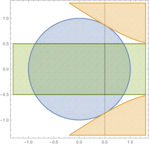
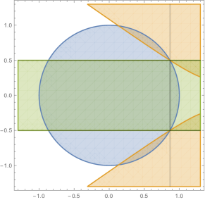
Figure 1 shows that the minimizers of over just the unit ball lie on the boundary at . Due to the linear constraints , these points are cut off from the feasible region. As a result, any minimizer of (i.e., the line ) inside the feasible region has norm strictly less than 1. Then by Corollary 3, the relaxation (4) is not tight.
2.3 Complexity of Solving Our Convex Reformulations
In this section, we explore the complexity of solving our convex relaxation/reformulation of TRS via FOMs. Our convex relaxation/reformulation of TRS (4) and its variants have the same domain as their original nonconvex counterparts (1) and thus are solvable via interior point methods and standard software as long as the cone has an explicit barrier function. However, because the standard polynomial-time interior point methods have expensive iterations in terms of their dependence on the problem dimension, here we mainly focus on FOMs with cheap iterations. We next discuss the complexity of solving our convex reformulation of the classical TRS given by (2) via Nesterov’s accelerated gradient descent algorithm [38], an optimal FOM for this class of problems. Once again, the main distinction between solving (4) as opposed to (5) via FOMs lies in how the projection onto the respective domain is handled. That is, whenever efficient projection onto the original domain is present, our discussion below will remain applicable to the conic case (4) as well.
The reformulation (5) of classical TRS (2) (or the convex relaxation (4) of TRS (1)) is an SOC program (convex program) and can easily be built whenever is available to us. Moreover, computing , the minimum eigenvalue of , itself is a TRS with no linear term because
There exist many efficient algorithms for computing the minimum eigenvalue of a symmetric matrix . One such algorithm that is effective for large sparse matrices is the Lanczos method [26, Chapter 10]. Implemented with a random start, this method enjoys the following probabilistic convergence guarantee (see [34, Section 4] and [29, Section 5]): with probability at least , the Lanczos method correctly estimates to within -accuracy in iterations. Furthermore, each iteration requires only matrix-vector products, and hence takes time, where is the number of nonzero entries in . Consequently, with probability at least , the randomized Lanczos method estimates to within -accuracy in time .
Given , problem (5) is simply minimizing a smooth convex quadratic function with smoothness parameter over the unit ball. Therefore, this problem can be efficiently solved using Nesterov’s accelerated gradient descent algorithm [38], which obtains an -accurate solution in iterations. This is the optimal rate for FOMs for solving this class of problems. The major computational burden in each iteration in these FOMs is the evaluation of the gradient of , which involves simply a matrix-vector product, and hence each iteration costs time. The only other main operation in each iteration of Nesterov’s algorithm applied to this problem is the projection onto the Euclidean ball, and this can be done in time. Consequently, Nesterov’s algorithm [38] applied to the optimization problem in our convex reformulation (5) of the classical TRS runs in time .
Thus, taking into account the complexity of computing to build our convex reformulation (5) and using Nesterov’s algorithm [38], we establish the following upper bound on the worst case number of elementary operations needed:
Theorem 10.
Remark 2.6.
This discussion shows that the classical TRS decomposes into two special TRS problems: one without a linear term, i.e., , making it a pure minimum eigenvalue problem, and the other one with a convex quadratic objective function. This once again highlights the connection between the TRS and eigenvalue problems, and in fact demonstrates that, up to constant factors, the complexity of solving the classical TRS is no worse than solving a minimum eigenvalue problem because the complexity in Theorem 10 is essentially determined by the complexity of computing minimum eigenvalue of a matrix. Rendl and Wolkowicz [43, Section 5] have empirically observed this connection between complexity of solving classical TRS and computing the minimum eigenvalue; our analysis complements their study with a theoretical justification.
Remark 2.7.
Using a deterministic algorithm to compute eliminates the probabilistic component in Theorem 10 at the expense of a slightly worse dependence on and in the iteration complexity.
Remark 2.8.
In practice, we will not be able to form the objective exactly, since will be computed only approximately. Let us consider an estimate and working with the objective . In Appendix A, we show that by using instead of , the error we incur is linearly dependent on the error of estimating with , which for our purposes is .
Remark 2.9.
Let us compare our bound (7) to the running time from [29]. The approach of [29, Theorem 1] requires
elementary operations to obtain an -accurate solution for (2) with probability , where . By using the convex reformulation (5) as opposed to the method of [29], we remove (at least) a factor of and the dependence on .
Our method is simpler to implement than the method of [29] as well because it decomposes the TRS into two well-studied problems as discussed in Remark 2.6. In contrast, since [29] relies on solving the dual SDP, at the end of its iterations, it requires additional operations to obtain the primal solution from the dual one, and then a rounding procedure to find the solution in the original space. Also, because the approach of [29] works in a lifted space and requires additional transformations at the end, it is not amenable to be used within the completely online convex optimization framework as described in [30].
3 Convexification of the Epigraph of TRS
In this section, we study the convex hull of the epigraph of TRS. In general, a tight convex relaxation for a nonconvex optimization problem does not necessarily imply that the epigraph of the convex relaxation is giving the exact convex hull of the epigraph of the nonconvex optimization problem. However, in the particular case of TRS with additional conic constraints, i.e., problem (1), under a slightly more stringent variant of Condition 2.1, we will establish that not only our convex relaxation given by (4) is tight but also its epigraph exactly characterizes the convex hull of the epigraph of underlying TRS (1) (see Corollary 14).
By defining a new variable (where the variable is reserved for later homogenization), and moving the nonconvex function from the objective to the constraints, we can equivalently recast (1) as minimizing over its epigraph
| (8) |
Since the objective is linear, optimizing over the epigraph is equivalent to optimizing over its convex hull. We define the associated epigraph as
| (9) |
Our convex hull characterizations are also SOC based. That is, as in Section 2.1, we focus mainly on the quadratic parts of the TRS (1), namely the nonconvex quadratic and the unit ball constraint and provide the convexification of this set via a single new SOC constraint.
Our approach is a refinement of the one from Burer and Kılınç-Karzan [16]. We first summarize the approach of [16] in Section 3.1 and then give our direct characterization in Section 3.2. As opposed to general SOCs and their cross-sections examined in Section 3.1, we present a direct study of in Section 3.2 that utilizes the fact that our domain in the context of TRS is a subset of an ellipsoid. Consequently, our analysis in Section 3.2 eliminates the need to verify several conditions from [16] completely and allows possibilities to handle additional conic constraints under appropriate assumptions. Finally, in Section 3.3, we extend our analysis to cover additional hollow constraints in the domain.
3.1 Summary and Discussion of Results from [16]
We start with a number of relevant definitions and conditions and then present the main result of [16].
A cone is said to be second-order-cone representable (or SOCr) if there exists a matrix and a vector such that the nonzero columns of are linearly independent, , and
| (10) |
Given an SOCr cone , the cone is also SOCr. Based on from (10), we define and consider the union . Note that corresponds to a nonconvex cone defined by the homogeneous quadratic inequality :
We define . Any matrix of the form as described above has exactly one negative eigenvalue, and given , we can recover by performing an eigenvalue decomposition of , see [16, Propositions 1 and 3].
Given matrices and a vector , we let for , and define the sets
Burer and Kılınç-Karzan [16] provide a general scheme to build an SOC-based convex relaxation of and establish that under appropriate conditions their relaxations are exactly describing and . Their analysis relies on the following conditions:
Condition 3.1.
has at least one positive eigenvalue and exactly one negative eigenvalue.
Condition 3.2.
There exists such that and .
Condition 3.3.
Either (i) is nonsingular, (ii) is singular and is positive definite on , or (iii) is singular and is negative definite on .
Conditions 3.1–3.3 ensure the existence of a maximal such that has a single negative eigenvalue for all , is invertible for all , and is singular—that is, is nontrivial whenever . Then, for all with , the set is well-defined by computing an eigenvalue decomposition of . We also need the following conditions on the value of :
Condition 3.4.
When , .
Condition 3.5.
When , or .
Conditions 3.1–3.5 are all that is needed to state the main result of [16]. Here, we state [16, Theorem 1] for completeness.
Theorem 11 ([16, Theorem 1]).
These convexification results were also applied to the classical TRS (2) in [16]. In particular, it is shown in [16, Section 7.2] that the classical TRS (2) can be reformulated in the form of
| (11) |
where and is defined to ensure and the multiplicity of in is at least two. Note that here . Then [16] suggests to solve (11) in two stages after the nonconvex domain in (11) is replaced by its convex hull. Specifically, [16] defines a new variable and the matrices
| (12) |
which then leads to
| (15) | ||||
| (19) | ||||
| (20) |
where and . Then the conditions of Theorem 11 are satisfied, and we deduce that there exists some ensuring
| (21) |
While the precise value of is not given in [16], one can show that in fact . We present the verification of conditions of Theorem 11 for matrices in (12) and the derivation for this value in Appendix B.
Remark 3.1.
The reformulation (11) of classical TRS (2) implicitly requires that because of the constraint . For the classical TRS (2) with no additional constraints, this is not an additional limitation because will always be a feasible solution with objective value and thus the optimum solution will have a nonpositive objective value. However, this becomes a limitation when we want to extend such arguments for the TRS (1) with additional conic constraints because may no longer be nonpositive.
3.2 Direct Convexification of the Epigraph of TRS
Due to Remark 3.1, we instead choose to study the epigraph of TRS (1) as in (9), which allows for positive objective values in (8) and avoids the additional lifting of the problem . To this end, we define the matrices
| (22) |
and the corresponding sets
| (23) | ||||
Note that , and thus is not convex. With these definitions, the epigraph from (9) can be written as
It is mentioned in [16] that the matrices (22) do not satisfy the necessary conditions to apply Theorem 11 directly. In particular, Condition 3.3 is violated for the choice of matrices (22). As a result, [16, Section 7.2] reformulates the classical TRS with matrices (12) instead. In contrast, we next show that in the special case of the classical TRS, via a direct analysis, finding the convex hull through linear aggregation of constraints will still carry through for the matrices in (22). This then indicates that while Condition 3.3 is sufficient, it is not necessary to obtain the convex hull result. In fact, we show that the value of that works for the matrices (12) will also work for our matrices (22). More precisely, for , we define
| (24) |
and prove that directly under the following condition that handles additional conic constraints.
Condition 3.6.
There exists a vector such that , , and .
Note that when is pointed and is full rank, Condition 3.6 assumes .
Remark 3.2.
One of the ingredients of our convex hull result is given in the next lemma.
Lemma 12.
Proof.
Let . Note that by definition, we have
where the last equation follows because , we have for all and then implies . As a result, holds for all . In addition, from these derivations, we immediately deduce that the set is an SOC representable set.
Proof.
We will first establish that . Since the sets are closed, this will immediately imply our closed convex hull result.
It is clear from the definition of and Lemma 12 that . We will prove the reverse direction.
Let be a vector in . Then satisfies
We will show that . If , then we are done. Suppose , that is, . Then from the definition of , , and , we have
Because , this implies . Let be the vector given by Condition 3.6 such that , , , and . We now consider the points for . We first argue that holds for all . To see this, note that
| (25) | ||||
where the third equation follows from and , and the inequality holds because and . Then from the inequality (3.2) and the definition of in (24), we conclude for all . Moreover, because and , there must exist such that . We define
Then by our choice of , we have . From , for all , and the relation
we conclude that for all such that . In particular, . Furthermore, by Condition 3.6, , and since is a cone, ; thus . Finally, in both , and so we have . Now it is easy to see that
As a consequence, we have the relation
By Lemma 12, the set is SOC representable and hence convex; this implies that is convex also. Then taking the convex hull of all terms in the above inequality gives us the result.
Note that the set is closed. We give our explicit convex hull result for TRS below.
Remark 3.3.
In the particular case of TRS with additional conic constraints, i.e., problem (1), under Condition 3.6, Corollary 14 shows that not only our convex relaxation given by (4) is tight but also we can characterize the convex hull of its epigraph exactly. Because Condition 3.6 holds for the classical TRS, this then recovers the results from [16, Section 6.2].
As a consequence of Remark 3.2 and Corollary 14, in all of the cases where Jeyakumar and Li [33] show the tightness of their convex reformulation, i.e., for robust least squares and robust SOC programming, we can further give the exact convex hull characterizations of the associated epigraphs.
We next present an example to illustrate that when Condition 3.6 is violated, we may not be able to obtain the convex hull description. We also give a variant of this example to demonstrate that there are cases where our convex relaxation is tight while Condition 3.6 is still violated.
Example 15.
Consider the following problem with the data given by
In this example, Condition 3.6 is violated. To see this, any vector such that is of the form . But then . Hence, if then , and similarly, if then .
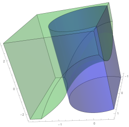
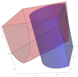
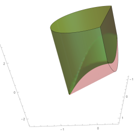
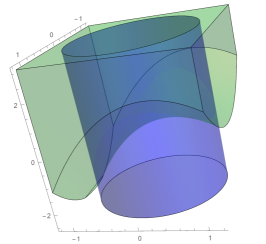
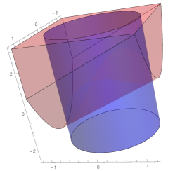
Figure 2(c) shows that the convex relaxation for the epigraph given by does not give the convex hull of . Note also that Condition 2.1 is satisfied for this example by taking , and so by Theorem 4, the SOC optimization problem (4) is a tight relaxation for (1). Despite this, we cannot give the exact convex hull characterization because Condition 3.6 is violated.
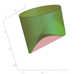
If we were to set instead of in this example, then the linear inequality would become redundant. In this case, our convex relaxation would give the convex hull, as illustrated in Figure 3 below. Nevertheless, even in this case Condition 3.6 would still be violated. This demonstrates that Condition 3.6 is not necessary to obtain the convex hull.
We close this section with a simple result which highlights a particularly important structure of the extreme points of .
Lemma 16.
Proof.
Consider with . Let be the vector given by Condition 3.6. Because satisfies and , for any ,
Now choose such that , and define . Then we have , since guarantees . Note that we will have and finite since and . Similarly, choosing such that , also. Then the point will be a convex combination of with weights and respectively.
3.3 Additional Hollow Constraints
In this section we explore additional constraints included in the domain of TRS (1), where and is a given possibly nonconvex set. More precisely, we characterize the convex hull of the set where , , , and are as defined in (3.2), and .
We impose the following condition on .
Condition 3.7.
The set satisfies .
Consider the case where is non-existent. If is a union of ellipsoids where each , then Condition 3.7 can be checked by solving
That is, satisfies Condition 3.7 if and only if . The computation of as stated requires solving a nonconvex quadratic program, which is nothing but a classical TRS after an appropriate affine transformation of the variables is applied. Hence, our developments from Section 2 give a tight SOC reformulation for it. In addition, the inhomogeneous -lemma [7, Proposition 3.5.2] ensures that the associated semidefinite relaxation is tight. Thus, Condition 3.7 can be verified efficiently when is a union of ellipsoids.
Hollow constraints have been studied in TRS literature under conditions similar to Condition 3.7. Most notably, the interval-bounded TRS [8, 11, 42, 49, 53] corresponds to the case when is a single lower-bounded quadratic constraint , where . The interval-bounded TRS is used to generate new steps in the context of the trust-region algorithm where minimum step lengths are enforced. In the case of interval-bounded TRS, Condition 3.7 is automatically satisfied. It is shown in a number of these papers [42, 53] that the natural SDP relaxation of interval-bounded TRS is tight. More recently, Yang et al. [52] showed the tightness of the SDP relaxation when the hollow set is the disjoint union of ellipsoids which do not intersect the boundary of the unit ball . As opposed to these results on tight SDP relaxations, Bienstock [10] has established that the general quadratically constrained quadratic programming problem
is polynomially solvable for a fixed number of constraints using a weak feasibility oracle, under the assumption that at least one quadratic constraint is strictly convex. In a similar vein, Bienstock and Michalka [12] also study TRS with additional ellipsoidal hollow constraints. Instead of giving the convex hull, [12] explores conditions that allow for polynomial solvability using a combinatorial enumeration technique and thus is able to cover cases where the set may not be contained in the unit ball. On a related subject, [11] studies the characterization and separation of valid linear inequalities that convexify the epigraph of a convex, differentiable function whose domain is restricted to the complement of a convex set defined by linear or convex quadratic inequalities.
We note that these papers [8, 10, 11, 12, 42, 49, 52, 53] consider the more general case of minimizing an arbitrary quadratic objective, which can be convex, over a domain given by possibly nonconvex quadratic constraints. On the other hand, our result applies to the special case of minimizing a nonconvex quadratic, i.e., , over the unit ball, a convex quadratic constraint. As a result, we are able to relax the assumptions that the set is generated by quadratics and the ellipsoidal hollows are disjoint. Specifically, we show that under Condition 3.7, our main convex hull result, i.e.,Theorem 13, obtained without the constraint is tight.
Theorem 17.
Proof.
Denoting , our aim is to prove . We trivially have . To prove , note that from Lemma 16, any point satisfies . Also, by Condition 3.7, the constraint does not remove any of the points with , in particular, all of the extreme points of are also in . Thus, . Moreover, because , the only recessive direction of is , i.e., . Note is also a recessive direction in . Then the result follows from
Theorem 17 has the following immediate implication.
Corollary 18.
Corollary 18 gives a convex reformulation for the interval-bounded TRS with , as do results from [8, 42, 49, 53]. These results were often derived as a consequence of a simultaneously diagonalizable assumption of the underlying matrices associated with TRS, or through SDP relaxations. In contrast to this, Condition 3.7 and Theorem 17 highlights the important geometric aspect, and provide a convex reformulation without additional variables. In addition, Corollary 18 together with Theorem 10 establish the convergence rate of FOMs to solve interval-bounded TRS as opposed to specialized algorithms suggested in [42].
Remark 3.4.
While preparing our first revision, an overlap of our original submission with a recent paper was brought to our attention. The first version of our work [31] was published online on March 10, 2016 on archives Optimization Online and arXiv and sent to a journal for possible publication. Five months after this date, on August 20, 2016, a paper by Jiulin Wang and Yong Xia [51] has appeared in online form on the journal Optimization Letters. It appears that this paper was submitted to Optimization Letters on March 21, 2016, 11 days after our paper was posted in public domain. To the best of our knowledge, Wang and Xia’s paper [51] was not available in public domain or available to us before August 20, 2016. The paper [51] has significant overlap with a part of the results in our paper. In particular, [51, Theorem 1] is a corollary of results in our original submission, see [31, Theorem 2.7 and Theorem 3.8]. Moreover, we were the first ones to note and discuss the use of Nesterov’s accelerated gradient descent algorithm in the context of TRS and demonstrate that it achieves the best-known theoretical convergence rate to solve TRS and some of its variants. Specifically, [31, Section 2.2] along with the conclusion of [31, Theorem 3.8] in the case of interval-bounded TRS covers not only [51, Section 3] but also highlights that there is no need to modify Nesterov’s accelerated gradient descent algorithm to solve exact convex reformulation of the interval-bounded TRS. Therefore, the convergence rate established in [31, Section 2.2] did already imply [51, Theorem 4]. To the best of our understanding, the main results in [51] are [51, Theorems 1 and 4]; whereas we also study SOC-based convex reformulations and convex hull descriptions of TRS and its variants with additional conic constraints and/or general hollow constraints see [31, Sections 2.1 and 3].
Acknowledgments
The authors wish to thank the review team for their constructive feedback that improved the presentation of the material in this paper. This research is supported in part by NSF grant CMMI 1454548.
References
- [1] S. Adachi, S. Iwata, Y. Nakatsukasa, and A. Takeda. Solving the trust region subproblem by a generalized eigenvalue problem. METR 2015-14, University of Tokyo, April 2015, 2015.
- [2] F. Alizadeh. Interior point methods in semidefinite programming with applications to combinatorial optimization. SIAM Journal on Optimization, 5(1):13–51, 1995.
- [3] A. Beck. Convexity properties associated with nonconvex quadratic matrix functions and applications to quadratic programming. Journal of Optimization Theory and Applications, 142(1):1–29, 2009.
- [4] A. Beck and Y. C. Eldar. Strong duality in nonconvex quadratic optimization with two quadratic constraints. SIAM Journal on Optimization, 17(3):844–860, 2006.
- [5] A. Ben-Tal and D. den Hertog. Hidden conic quadratic representation of some nonconvex quadratic optimization problems. Mathematical Programming, 143(1):1–29, 2014.
- [6] A. Ben-Tal, L. El Ghaoui, and A. Nemirovski. Robust Optimization. Princeton University Press. Princeton Series in Applied Mathematics, Philadelphia, PA, USA, 2009.
- [7] A. Ben-Tal and A. Nemirovski. Lectures on modern convex optimization. Technical report, August 2015. http://www2.isye.gatech.edu/~nemirovs/Lect_ModConvOpt.pdf.
- [8] A. Ben-Tal and M. Teboulle. Hidden convexity in some nonconvex quadratically constrained quadratic programming. Mathematical Programming, 72(1):51–63, 1996.
- [9] D. Bertsimas, D. B. Brown, and C. Caramanis. Theory and applications of robust optimization. SIAM Review, 53(3):464–501, 2011.
- [10] D. Bienstock. A note on polynomial solvability of the CDT problem. SIAM Journal on Optimization, 26(1):488–498, 2016.
- [11] D. Bienstock and A. Michalka. Cutting-planes for optimization of convex functions over nonconvex sets. SIAM Journal on Optimization, 24(2):643–677, 2014.
- [12] D. Bienstock and A. Michalka. Polynomial solvability of variants of the trust-region subproblem. In Proceedings of the Twenty-Fifth Annual ACM-SIAM Symposium on Discrete Algorithms, pages 380–390, 2014.
- [13] C. Buchheim, M. De Santis, L. Palagi, and M. Piacentini. An exact algorithm for nonconvex quadratic integer minimization using ellipsoidal relaxations. SIAM Journal on Optimization, 23(3):1867–1889, 2013.
- [14] S. Burer. A gentle, geometric introduction to copositive optimization. Mathematical Programming, 151(1):89–116, 2015.
- [15] S. Burer and K. M. Anstreicher. Second-order-cone constraints for extended trust-region subproblems. SIAM Journal on Optimization, 23(1):432–451, 2013.
- [16] S. Burer and F. Kılınç-Karzan. How to convexify the intersection of a second order cone and a nonconvex quadratic. Mathematical Programming, July 2016.
- [17] S. Burer and B. Yang. The trust region subproblem with non-intersecting linear constraints. Mathematical Programming, 149(1):253–264, 2014.
- [18] M. Celis, J. Dennis, and R. Tapia. A trust region strategy for nonlinear equality constrained optimization. In Numerical Optimization 1984: Proceedings of the SIAM Conference on Numerical Optimization, pages 71–82. SIAM Philadelphia, PA, 1985.
- [19] A. R. Conn, N. I. M. Gould, and P. L. Toint. Trust-Region Methods. MPS/SIAM Series on Optimization. SIAM, Philadelphia, PA, 2000.
- [20] L. L. Dines. On the mapping of quadratic forms. Bulletin of the American Mathematical Society, 47(6):494–498, 06 1941.
- [21] J. B. Erway and P. E. Gill. A subspace minimization method for the trust-region step. SIAM Journal on Optimization, 20(3):1439–1461, 2010.
- [22] J. B. Erway, P. E. Gill, and J. D. Griffin. Iterative methods for finding a trust-region step. SIAM Journal on Optimization, 20(2):1110–1131, 2009.
- [23] C. Fortin and H. Wolkowicz. The trust region subproblem and semidefinite programming. Optimization Methods and Software, 19(1):41–67, 2004.
- [24] A. L. Fradkov and V. A. Yakubovich. The S-procedure and duality relations in nonconvex problems of quadratic programming. Vestn. LGU, Ser. Mat., Mekh., Astron, (1):101–109, 1979.
- [25] W. Gander, G. H. Golub, and U. von Matt. A constrained eigenvalue problem. Linear Algebra and its Applications, 114–115:815 – 839, 1989. Special Issue Dedicated to Alan J. Hoffman.
- [26] G. H. Golub and C. F. Van Loan. Matrix Computations. Johns Hopkins studies in the mathematical sciences. The Johns Hopkins University Press, Baltimore, London, 1996.
- [27] N. I. M. Gould, S. Lucidi, M. Roma, and P. L. Toint. Solving the trust-region subproblem using the Lanczos method. SIAM Journal on Optimization, 9(2):504–525 (electronic), 1999.
- [28] N. I. M. Gould, D. P. Robinson, and H. S. Thorne. On solving trust-region and other regularized subproblems in optimization. Mathematical Programming Computation, 2(1):21–57, 2010.
- [29] E. Hazan and T. Koren. A linear-time algorithm for trust region problems. Mathematical Programming, 158(1):363–381, 2016.
- [30] N. Ho-Nguyen and F. Kılınç-Karzan. Online first-order framework for robust convex optimization. Technical report, July 2016. http://www.optimization-online.org/DB_HTML/2016/07/5555.html.
- [31] N. Ho-Nguyen and F. Kılınç-Karzan. A second-order cone based approach for solving the trust region subproblem and its variants. Technical report, March 10 2016. http://www.optimization-online.org/DB_HTML/2016/03/5362.html, https://arxiv.org/abs/1603.03366v1.
- [32] R. A. Horn and C. R. Johnson. Matrix analysis. Cambridge University Press, New York, 2013.
- [33] V. Jeyakumar and G. Y. Li. Trust-region problems with linear inequality constraints: Exact SDP relaxation, global optimality and robust optimization. Mathematical Programming, 147(1):171–206, 2013.
- [34] J. Kuczynski and H. Wozniakowski. Estimating the largest eigenvalue by the power and lanczos algorithms with a random start. SIAM Journal on Matrix Analysis and Applications, 13(4):1094–1122, 1992.
- [35] M. Locatelli. Exactness conditions for an sdp relaxation of the extended trust region problem. Optimization Letters, 10(6):1141–1151, 2016.
- [36] S. Modaresi and J. Vielma. Convex hull of two quadratic or a conic quadratic and a quadratic inequality. Technical report, November 2014. http://www.optimization-online.org/DB_HTML/2014/11/4641.html.
- [37] J. J. Moré and D. C. Sorensen. Computing a trust region step. SIAM Journal on Scientific and Statistical Computing, 4(3):553–572, 1983.
- [38] Y. Nesterov. A method for solving a convex programming problem with rate of convergence . Soviet Math. Dokl., 27(2):372–376, 1983.
- [39] Y. Nesterov and A. Nemirovski. Interior-Point Polynomial Algorithms in Convex Programming. Society for Industrial and Applied Mathematics, 1994.
- [40] J. Nocedal and S. Wright. Numerical Optimization. Springer Series in Operations Research and Financial Engineering. Springer New York, 2000.
- [41] I. Pólik and T. Terlaky. A survey of the s-lemma. SIAM Review, 49(3):371–418, 2007.
- [42] T. K. Pong and H. Wolkowicz. The generalized trust region subproblem. Computational Optimization and Applications, 58(2):273–322, 2014.
- [43] F. Rendl and H. Wolkowicz. A semidefinite framework for trust region subproblems with applications to large scale minimization. Mathematical Programming, 77(2):273–299, 1997.
- [44] M. Rojas, S. A. Santos, and D. C. Sorensen. A new matrix-free algorithm for the large-scale trust-region subproblem. SIAM Journal on Optimization, 11(3):611–646, 2001.
- [45] M. Salahi and S. Fallahi. Trust region subproblem with an additional linear inequality constraint. Optimization Letters, 10(4):821–832, 2016.
- [46] M. Salahi and A. Taati. A fast eigenvalue approach for solving the trust region subproblem with an additional linear inequality. Computational and Applied Mathematics, pages 1–19, 2015.
- [47] M. Salahi, A. Taati, and H. Wolkowicz. Local nonglobal minima for solving large-scale extended trust-region subproblems. Computational Optimization and Applications, pages 1–22, 2016.
- [48] D. C. Sorensen. Minimization of a large-scale quadratic function subject to a spherical constraint. SIAM Journal on Optimization, 7(1):141–161, 1997.
- [49] R. J. Stern and H. Wolkowicz. Indefinite trust region subproblems and nonsymmetric eigenvalue perturbations. SIAM Journal on Optimization, 5(2):286–313, 1995.
- [50] J. F. Sturm and S. Zhang. On cones of nonnegative quadratic functions. Mathematics of Operations Research, 28(2):246–267, 2003.
- [51] J. Wang and Y. Xia. A linear-time algorithm for the trust region subproblem based on hidden convexity. Optimization Letters, http://link.springer.com/article/10.1007/s11590-016-1070-0, August August 2016.
- [52] B. Yang, K. Anstreicher, and S. Burer. Quadratic programs with hollows. Technical report, January 2016. http://www.optimization-online.org/DB_FILE/2016/01/5277.pdf.
- [53] Y. Ye and S. Zhang. New results on quadratic minimization. SIAM Journal on Optimization, 14(1):245–267, 2003.
- [54] H. Zhang, A. R. Conn, and K. Scheinberg. A derivative-free algorithm for least-squares minimization. SIAM Journal on Optimization, 20(6):3555–3576, 2010.
Appendix A Working with Approximate Eigenvalues
Consider the classical TRS (2) and its convex reformulation (5). In practice, we will actually form the objective where is an approximation. Due to this imprecision, we must ensure that the objective remains convex. To do this, suppose that we solve the minimum eigenvalue problem of to within -accuracy, and obtain an approximate solution . Subtracting from the inequality, we obtain . To ensure the convexity of the objective, we set which is an underestimate of , ensuring that . Let which satisfies , and
Based on this scheme, we next explore the effects of solving
| (26) |
instead of (5). Let be an optimal solution to the true convex reformulation (5). Let be an optimal solution to (26) and be an approximate optimal solution. Then we can bound the objective value as
where the last inequality follows from and . Thus, the convergence rate of to the optimum of (5) is controlled by the size of and the convergence rate for solving (26).
We can also control the distance between and . Because is a -strongly convex function, we have
where the last inequality follows from the optimality of for the problem (26), i.e., , and the optimality of for the problem (5). Then . Also, from , we deduce that if , then . When , the only constraint in our domain is inactive, and thus we conclude that is also optimum for the unconstrained minimization problem. Then the optimality conditions leads to . This implies that . Moreover, satisfies the optimality condition for all such that . Since our domain is the unit ball, this is true if and only if , for some . Therefore, , where denotes the pseudo-inverse of a matrix . If we denote the ordered eigenvalues of by and their corresponding orthonormal eigenvectors by , we obtain
Note that it is possible to have and . However, this happens only when , so we follow the convention . After some simple algebra, we have the equality
Since and , we must have . Also, is possible only if . Hence, we have
This shows that , where . Therefore,
Thus has error , which is expected since the error in the objective function is , and the objective function is quadratic.
Appendix B Computation of value
Recall the notation and . For the set in (15), Condition 3.1 is satisfied by construction, and Condition 3.2 is satisfied by taking with , , and . This ensures that for any , we have
| (27) |
and . Thus, by the variational characterization of eigenvalues, has at least one negative eigenvalue. Also, Condition 3.3(ii) is now satisfied.
We next show that the precise value of is simply determined by .
Lemma 19.
Proof.
Define . From (27), note that has a block structure and is such that it equals to the smallest positive ensuring
is singular.
Let be the two smallest eigenvalues of , and be the two smallest eigenvalues of . Notice that has the same eigenvectors as , and the eigenvalues are simply scaled and shifted from those of , thus the minimum eigenvalue of is for . Also, by construction, the multiplicity of in is at least two, so the multiplicity of the minimum eigenvalue of is also at least two, therefore .
For any , the last diagonal entry of is negative implying is not positive semidefinite, hence . However, for , , and from Cauchy’s interlacing theorem for eigenvalues [32, Theorem 4.3.17], we obtain
Thus, for any , the matrix , and hence , is invertible, and has exactly one negative eigenvalue. When , . By recalling that and , we immediately observe that , and thus , is singular since has eigenvector with eigenvalue . Also,
so has exactly one negative eigenvalue. Moreover, for any , the minimum eigenvalue of is . Hence, for any , follows from [32, Theorem 4.3.17]. As a result , and thus , has at least two negative eigenvalues. Therefore, is the correct value.