Improved convergence rates for Lasserre-type hierarchies of upper bounds for box-constrained polynomial optimization

Abstract

We consider the problem of minimizing a given $n$-variate polynomial $f$ over the hypercube $[-1,1]^{n}$. An idea introduced by Lasserre, is to find a probability distribution on $[-1,1]^{n}$ with polynomial density function $h$ (of given degree $r$) that minimizes the expectation $\int_{[-1,1]^{n}}f(x)h(x)d\mu(x)$, where $d\mu(x)$ is a fixed, finite Borel measure supported on $[-1,1]^{n}$. It is known that, for the Lebesgue measure $d\mu(x)=dx$, one may show an error bound $O(1/\sqrt{r})$ if $h$ is a sum-of-squares density, and an $O(1/r)$ error bound if $h$ is the density of a beta distribution. In this paper, we show an error bound of $O(1/r^{2})$, if $d\mu(x)=\left(\prod_{i=1}^{n}\sqrt{1-x_{i}^{2}}\right)^{-1}dx$ (the well-known measure in the study of orthogonal polynomials), and $h$ has a Schmüdgen-type representation with respect to $[-1,1]^{n}$, which is a more general condition than a sum of squares. The convergence rate analysis relies on the theory of polynomial kernels and, in particular, on Jackson kernels. We also show that the resulting upper bounds may be computed as generalized eigenvalue problems, as is also the case for sum-of-squares densities.

Keywords: box-constrained global optimization, polynomial optimization, Jackson kernel, semidefinite programming, generalized eigenvalue problem, sum-of-squares polynomial

AMS classification: 90C60, 90C56, 90C26.

1 Introduction

1.1 Background results

We consider the problem of minimizing a given $n$-variate polynomial $f\in\mathbb{R}[x]$ over the compact set ${\mathbf{K}}=[-1,1]^{n}$, i.e., computing the parameter

$$f_{\min} = \min_{x\in{\mathbf{K}}}f(x).$$ (1.1)

This is a hard optimization problem which contains, e.g., the well-known NP-hard maximum stable set and maximum cut problems in graphs (see, e.g., [15, 16]). It falls within box-constrained (aka bound-constrained) optimization which has been widely studied in the literature. In particular iterative methods for bound-constrained optimization are described in the books [1, 5, 6], including projected gradient and active set methods. The latest algorithmic developments for box-constrained global optimization are surveyed in the recent thesis [14]; see also [7] and the references therein for recent work on active set methods, and a list of applications. The box-constrained optimization problem is even of practical interest in the (polynomially solvable) case where $f$ is a convex quadratic problem, and dedicated active set methods have been developed for this case; see [8].

In this paper we will focus on the question of finding a sequence of upper bounds converging to the global minimum and allowing a known estimate on the rate of convergence. It should be emphasized that it is in general a difficult challenge in non-convex optimization to obtain such results. Following Lasserre [9, 10], our approach will be based on reformulating problem (1.1) as an optimization problem over measures and then restricting it to subclasses of measures that we are able to analyze. Sequences of upper bounds have been recently proposed and analyzed in [4, 3]; in the present paper we will propose new bounds for which we can prove a sharper rate of convergence. We now introduce our approach.

As observed by Lasserre [9], problem (1.1) can be reformulated as

$$f_{\min} = \min_{\mu\in\mathcal{M}({\mathbf{K}})}\int_{{\mathbf{K}}}f(x)d\mu(x),$$

where $\mathcal{M}({\mathbf{K}})$ denotes the set of probability measures supported on ${\mathbf{K}}$. Hence an upper bound on $f_{\min}$ may be obtained by considering a fixed probability measure $\mu$ on ${\mathbf{K}}$. In particular, the optimal value $f_{\min}$ is obtained when selecting for $\mu$ the Dirac measure at a global minimizer $x^{*}$ of $f$ in ${\mathbf{K}}$.

Lasserre [10] proposed the following strategy to build a hierarchy of upper bounds converging to $f_{\min}$. The idea is to do successive approximations of the Dirac measure at $x^{*}$ by using sum-of-squares (SOS) density functions of growing degrees. More precisely, Lasserre [10] considered a set of Borel measures $\mu_{r}$ obtained by selecting a fixed, finite Borel measure $\mu$ on ${\mathbf{K}}$ (like, e.g., the Lebesgue measure) together with a polynomial density function that is a sum-of-squares (SOS) polynomial of given degree $r$.

When selecting for $\mu$ the Lebesgue measure on ${\mathbf{K}}$ this leads to the following hierarchy of upper bounds on $f_{\min}$, indexed by $r\in{\mathbb{N}}$:

$$\underline{f}^{(r)}_{\mathbf{K}}:=\inf_{h\in\Sigma[x]_{r}}\int_{\mathbf{K}}h(x)f(x)dx\ \ \text{s.t. $\int_{\mathbf{K}}h(x)dx=1$,}$$ (1.2)

where $\Sigma[x]_{r}$ denotes the set of sum-of-squares polynomials of degree at most $r$.

The convergence to $f_{\min}$ of the bounds $\underline{f}^{(r)}_{{\mathbf{K}}}$ is an immediate consequence of the following theorem, which holds for general compact sets ${\mathbf{K}}$ and continuous functions $f$.

Theorem 1.1

[10, cf. Theorem 3.2] Let $\mathbf{K}\subseteq{\mathbb{R}}^{n}$ be compact, let $\mu$ be an arbitrary finite Borel measure supported by $\mathbf{K}$, and let $f$ be a continuous function on ${\mathbb{R}}^{n}$. Then, $f$ is nonnegative on $\mathbf{K}$ if and only if

$$\int_{\mathbf{K}}fg^{2}d\mu\geq 0\ \ \forall g\in{\mathbb{R}}[x].$$

Therefore, the minimum of $f$ over $\mathbf{K}$ can be expressed as

$$f_{\min}=\inf_{h\in\Sigma[x]}\int_{\mathbf{K}}fhd\mu\ \ \text{s.t. $\int_{\mathbf{K}}hd\mu=1$.}$$ (1.3)

As already mentioned in [4], formula (1.3) does not appear explicitly in [10] which only mentions the characterization of nonnegative functions, but one can derive it easily from this nonnegativity characterization. To see this we write $f_{\min}=\sup\{\lambda:f(x)-\lambda\geq 0\text{ on }\mathbf{K}\}$. Then, for any finite Borel measure $\mu$, we have $f_{\min}=\sup\{\lambda:\int_{\mathbf{K}}h(f-\lambda)d\mu\geq 0\ \forall h\in\Sigma[x]\}$. As $\int_{\mathbf{K}}h(f-\lambda)d\mu=\int_{\mathbf{K}}hf\,d\mu-\lambda\int_{\mathbf{K}}h\,d\mu$, after normalizing $\int_{\mathbf{K}}h\,d\mu=1$, the formula (1.3) follows.

In the recent work [3], it is shown that for a compact set $\mathbf{K}\subseteq[0,1]^{n}$ one may obtain a similar result using density functions arising from (products of univariate) beta distributions. In particular, the following theorem is implicit in [3].

Theorem 1.2

[3] Let $\mathbf{K}\subseteq[0,1]^{n}$ be a compact set, let $\mu$ be an arbitrary finite Borel measure supported by $\mathbf{K}$, and let $f$ be a continuous function on ${\mathbb{R}}^{n}$. Then, $f$ is nonnegative on $\mathbf{K}$ if and only if

$$\int_{\mathbf{K}}fhd\mu\geq 0$$

for all $h$ of the form

$$h(x)=\frac{\prod_{i=1}^{n}x_{i}^{\beta_{i}}(1-x_{i})^{\eta_{i}}}{\int_{{\mathbf{K}}}\prod_{i=1}^{n}x_{i}^{\beta_{i}}(1-x_{i})^{\eta_{i}}},$$ (1.4)

where the $\beta_{i}^{\prime}$s and $\eta_{i}^{\prime}$s are nonnegative integers. Therefore, the minimum of $f$ over $\mathbf{K}$ can be expressed as

$$f_{\min}=\inf_{h}\int_{\mathbf{K}}fhd\mu\ \ \text{s.t. $\int_{\mathbf{K}}hd\mu=1$,}$$ (1.5)

where the infimum is taken over all beta-densities $h$ of the form (1.4).

For the box ${\mathbf{K}}=[0,1]^{n}$ and selecting for $\mu$ the Lebesgue measure, we obtain a hierarchy of upper bounds $f^{H}_{r}$ converging to $f_{\min}$, where $f^{H}_{r}$ is the optimum value of the program (1.5) when the infimum is taken over all beta-densities $h$ of the form (1.4) with degree $r$.

The rate of convergence of the upper bounds $\underline{f}^{(r)}_{\mathbf{K}}$ and $f^{H}_{r}$ has been investigated recently in [4] and [3], respectively. It is shown in [4] that $\underline{f}^{(r)}_{\mathbf{K}}-f_{\min}=O(1/\sqrt{r})$ for a large class of compact sets ${\mathbf{K}}$ (including all convex bodies and thus the box $[0,1]^{n}$ or $[-1,1]^{n}$) and the stronger rate $f^{H}_{r}-f_{\min}=O(1/r)$ is shown in [3] for the box ${\mathbf{K}}=[0,1]^{n}$. While the parameters $\underline{f}^{(r)}_{{\mathbf{K}}}$ can be computed using semidefinite optimization (in fact, a generalized eigenvalue computation problem, see [10]), an advantage of the parameters $f^{H}_{r}$ is that their computation involves only elementary operations (see [3]).

Another possibility for getting a hierarchy of upper bounds is grid search, where one takes the best function evaluation at all rational points in $\mathbf{K}=[0,1]^{n}$ with given denominator $r$. It has been shown in [3] that these bounds have a rate of convergence in $O(1/r^{2})$. However, the computation of the order $r$ bound needs an exponential number $r^{n}$ of function evaluations.

1.2 New contribution

In the present work we continue this line of research. For the box ${\mathbf{K}}=[-1,1]^{n}$, our objective is to build a new hierarchy of measure-based upper bounds, for which we will be able to show a sharper rate of convergence in $O(1/r^{2})$. We obtain these upper bounds by considering a specific Borel measure $\mu$ (specified below in (1.7)) and polynomial density functions with a so-called Schmüdgen-type SOS representation (as in (1.6) below).

We first recall the relevant result of Schmüdgen [20], which gives SOS representations for positive polynomials on a basic closed semi-algebraic set (see also, e.g., [18],[11, Theorem 3.16], [13]).

Theorem 1.3 (Schmüdgen [20])

Consider the set $\mathbf{K}=\{{x}\in\mathbb{R}^{n}\mid g_{1}(x)\geq 0,\dotsc,g_{m}(x)\geq 0\}$, where $g_{1},\dotsc,g_{m}\in\mathbb{R}[{x}]$, and assume that ${\mathbf{K}}$ is compact. If $p\in\mathbb{R}[x]$ is positive on ${\mathbf{K}}$, then $p$ can be written as $p=\sum_{I\subseteq[m]}\sigma_{I}\prod_{i\in I}g_{i}$, where $\sigma_{I}$ ($I\subseteq[m]$) are sum-of-squares polynomials.

For the box ${\mathbf{K}}=[-1,1]^{n}$, described by the polynomial inequalities $1-x_{1}^{2}\geq 0,\ldots,1-x_{n}^{2}\geq 0$, we consider polynomial densities that allow a Schmüdgen-type representation of bounded degree $r$:

$$h(x)=\sum_{I\subseteq[n]}\sigma_{I}(x)\prod_{i\in I}(1-x_{i}^{2}),$$ (1.6)

where the polynomials $\sigma_{I}$ are sum-of-squares polynomials with degree at most $r-2|I|$ (to ensure that the degree of $h$ is at most $r$). We will also fix the following Borel measure $\mu$ on $[-1,1]^{n}$ (which, as will be recalled below, is associated with some orthogonal polynomials):

$$d\mu(x)=\left(\prod_{i=1}^{n}\pi\sqrt{1-x_{i}^{2}}\right)^{-1}dx.$$ (1.7)

This leads to the following new hierarchy of upper bounds ${f}^{(r)}$ for $f_{\min}$.

Definition 1.4

Let $\mu$ be the Borel measure from (1.7). For $r\in{\mathbb{N}}$ consider the parameters

$${f}^{(r)}:=\inf_{h}\int_{[-1,1]^{n}}fhd\mu\ \ \text{s.t. $\int_{[-1,1]^{n}}hd\mu=1$,}$$ (1.8)

where the infimum is taken over the polynomial densities $h$ that allow a Schmüdgen-type representation (1.6), where each $\sigma_{I}$ is a sum-of-squares polynomial with degree at most $r-2|I|$.

The convergence of the parameters $f^{(r)}$ to $f_{\min}$ follows as a direct application of Theorem 1.1, since $f_{\min}\leq f^{(r+1)}\leq f^{(r)}$ for all $r$ and sums of squares allow a Schmüdgen-type representation. As a small remark, note that due to the fact that $[-1,1]^{n}$ has a nonempty interior the program (1.8) has an optimal solution $h^{*}$ for all $r$ by [10, Theorem 4.2].

A main result in this paper is to show that the bounds $f^{(r)}$ have a rate of convergence in $O(1/r^{2})$. Moreover we will show that the parameter $f^{(r)}$ can be computed through generalized eigenvalue computations.

Theorem 1.5

Let $f\in{\mathbb{R}}[x]$ be a polynomial and $f_{\min}$ be its minimum value over the box $[-1,1]^{n}$. For any $r$ large enough, the parameters $f^{(r)}$ defined in (1.8) satisfy

$$f^{(r)}-f_{\min}=O\left(\frac{1}{r^{2}}\right).$$

As already observed above this result compares favorably with the estimate: $\underline{f}^{(r)}_{\mathbf{K}}-f_{\min}=O\left(\frac{1}{\sqrt{r}}\right)$ shown in [4] for the bounds $f^{(r)}_{{\mathbf{K}}}$ based on using SOS densities. (Note however that the latter convergence rate holds for a larger class of sets $\mathbf{K}$ that includes all convex bodies; see [4] for details.) The new result also improves the estimate $f^{H}_{r}-f_{\min}=O\left(\frac{1}{{r}}\right)$, shown in [3] for the bounds $f^{H}_{r}$ obtained by using densities arising from beta distributions.

We now illustrate the optimal densities appearing in the new bounds $f^{(r)}$ on an example.

Example 1.6

Consider the minimization of the Motzkin polynomial

$$f(x_{1},x_{2})=64(x_{1}^{4}x_{2}^{2}+x_{1}^{2}x_{2}^{4})-48x_{1}^{2}x_{2}^{2}+1$$

over the hypercube $[-1,1]^{2}$, which has four global minimizers at the points $\left(\pm\frac{1}{2},\pm\frac{1}{2}\right)$, and $f_{\min}=0$. Figure 1 shows the optimal density function $h^{*}$ computed when solving the problem (1.8) for degrees $12$ and $16$, respectively. Note that the optimal density $h^{*}$ shows four peaks at the four global minimizers of $f$ in $[-1,1]^{2}$. The corresponding upper bounds from (1.8) are $f^{(12)}=0.8098$ and $f^{(16)}=0.6949$.

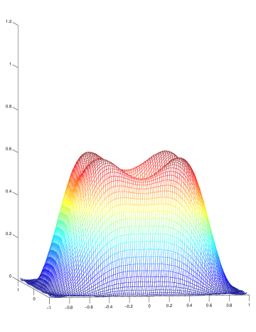
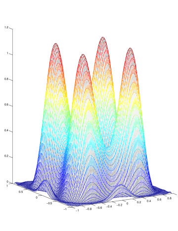
Figure 1: Graphs of $h^{*}$ on $[-1,1]^{2}$ ($\deg(h^{*})=12,16$) for the Motzkin polynomial.

Strategy and outline of the paper

In order to show the convergence rate in $O(1/r^{2})$ of Theorem 1.5 we need to exhibit a polynomial density function $h_{r}$ of degree at most $r$ which admits an SOS representation of Schmüdgen-type and for which we are able to show that $\int_{[-1,1]^{n}}fhd\mu-f_{\min}=O(1/r^{2}).$ The idea is to find such a polynomial density which approximates well the Dirac delta function at a global minimizer $x^{*}$ of $f$ over $[-1,1]^{n}$. For this we will use the well-established polynomial kernel method (KPM) and, more specifically, we will use the Jackson kernel, a well known tool in approximation theory to yield best (uniform) polynomial approximations of continuous functions.

The paper is organized as follows. Section 2 contains some background information about the polynomial kernel method needed for our analysis of the new bounds $f^{(r)}$. Specifically, we introduce Chebyshev polynomials in Section 2.1 and Jackson kernels in Section 2.2, and then we use them in Section 2.3 to construct suitable polynomial densities $h_{r}$ giving good approximations of the Dirac delta function at a global minimizer of $f$ in the box. We then carry out the analysis of the upper bounds on $f_{\min}$ in Section 3.1 for the univariate case and in Section 3.2 for the general multivariate case, thus proving the result of Theorem 1.5. In Section 4 we show how the new bounds $f^{(r)}$ can be computed as generalized eigenvalue problems and in Section 5 we conclude with some numerical examples illustrating the behavior of the bounds $f^{(r)}$.

Notation

Throughout, $\Sigma[x]$ denotes the set of all sum-of-squares (SOS) polynomials (i.e., all polynomials $h$ of the form $h=\sum_{i=1}^{k}p_{i}(x)^{2}$ for some polynomials $p_{1},\ldots,p_{k}$ and $k\in{\mathbb{N}}$) and $\Sigma[x]_{r}$ denotes the set of SOS polynomials of degree at most $r$ (of the form $h=\sum_{i=1}^{k}p_{i}(x)^{2}$ for some polynomials $p_{i}$ of degree at most $r/2$). For $\alpha\in{\mathbb{N}}^{n}$, $\text{\rm Supp}(\alpha)=\{i\in[n]:\alpha_{i}\neq 0\}$ denotes the support of $\alpha$ and, for $\alpha,\beta\in{\mathbb{N}}^{n}$, $\delta_{\alpha,\beta}\in\{0,1\}$ is equal to 1 if and only if $\alpha=\beta$.

2 Background on the polynomial kernel method

Our goal is to approximate the Dirac delta function at a given point $x^{*}\in{\mathbb{R}}^{n}$ as well as possible, using polynomial density functions of bounded degrees. This is a classical question in approximation theory. In this section we will review how this may be done using the polynomial kernel method and, in particular, using Jackson kernels. This theory is usually developed using the Chebyshev polynomials, and we start by reviewing their properties. We will follow mainly the work [21] for our exposition and we refer to the handbook [2] for more background information.

2.1 Chebyshev polynomials

We will use the univariate polynomials $T_{k}(x)$ and $U_{k}(x)$, respectively known as the Chebyshev polynomials of the first and second kind. They are defined as follows:

$$T_{k}(x)=\cos(k\arccos(x)),\ \ \ U_{k}(x)=\frac{\sin((k+1)\arccos(x))}{\sin(\arccos(x))}\ \ \text{ for }\ x\in[-1,1],\ k\in{\mathbb{N}},$$ (2.1)

and they satisfy the following recurrence relationships:

$$T_{0}(x)=1,\ T_{-1}(x)=T_{1}(x)=x,\ T_{k+1}(x)=2xT_{k}(x)-T_{k-1}(x),$$ (2.2)

$$U_{0}(x)=1,\ U_{-1}(x)=0,\ U_{k+1}(x)=2xU_{k}(x)-U_{k-1}(x).$$ (2.3)

As a direct application one can verify that

$$\begin{split}T_{k}(0)&=\begin{cases}0&\text{ for }k\text{ odd},\\ (-1)^{\frac{k}{2}}&\text{ for }k\text{ even},\end{cases}\\ T_{k}(1)&=1,\ U_{k}(1)=k+1,\ U_{k}(-1)=(-1)^{k}(k+1)\ \ \ \text{ for }k\in{\mathbb{N}}.\end{split}$$ (2.4)

The Chebyshev polynomials have the extrema

$$\max_{x\in[-1,1]}|T_{k}(x)|=1\mbox{ and }\max_{x\in[-1,1]}|U_{k}(x)|=k+1,$$

attained at $x=\pm 1$ (see, e.g., [2, §22.14.4, 22.14.6]).

The Chebyshev polynomials are orthogonal for the following inner product on the space of integrable functions over $[-1,1]$:

$$\langle f,g\rangle=\int_{-1}^{1}\frac{f(x)g(x)}{\pi\sqrt{1-x^{2}}}dx,$$ (2.5)

and their orthogonality relationships read

$$\langle T_{k},T_{m}\rangle=0\text{ if }k\neq m,\ \langle T_{0},T_{0}\rangle=1,\ \langle T_{k},T_{k}\rangle=\tfrac{1}{2}\ \text{ if }k\geq 1.$$ (2.6)

For any $r\in{\mathbb{N}}$ the Chebyshev polynomials $T_{k}$ ($k\leq r$) form a basis of the space of univariate polynomials with degree at most $r$. One may write the Chebyshev polynomials in the standard monomial basis using the relations

$$T_{k}(x) =\sum_{i=0}^{k}t_{i}^{(k)}x^{i}=\frac{k}{2}\sum_{m=0}^{\lfloor\frac{k}{2}\rfloor}(-1)^{m}\frac{(k-m-1)!}{m!(k-2m)!}(2x)^{k-2m}, k>0$$

$$U_{k-1}(x) =\sum_{i=0}^{k-1}u_{i}^{(k)}x^{i}=\sum_{m=0}^{\lfloor\frac{k-1}{2}\rfloor}(-1)^{m}\frac{(k-m-1)!}{m!(k-1-2m)!}(2x)^{k-1-2m}, k>1;$$

see, e.g., [2, Chap. 22]. From this, one may derive a bound on the largest coefficient in absolute value appearing in the above expansions of $T_{k}(x)$ and $U_{k-1}(x)$. A proof for the following result will be given in the appendix.

Lemma 2.1

For any fixed integer $k>1$, one has

$$\max_{0\leq i\leq k-1}|u_{i}^{(k)}|\leq\max_{0\leq i\leq k}|t_{i}^{(k)}|=2^{k-1-2\psi(k)}\frac{k(k-\psi(k)-1)!}{\psi(k)!(k-2\psi(k))!},$$ (2.7)

where $\psi(k)=0$ for $k\leq 4$ and $\psi(k)=\left\lceil\frac{1}{8}\left(4k-5-\sqrt{8k^{2}-7}\right)\right\rceil$ for $k\geq 4$. Moreover, the right-hand side of (2.7) increases monotonically with increasing $k$.

In the multivariate case we use the following notation. We let $d\mu(x)$ denote the Lebesgue measure on $[-1,1]^{n}$ with the function $\prod_{i=1}^{n}\left(\pi\sqrt{1-x_{i}^{2}}\right)^{-1}$ as density function:

$$d\mu(x)=\prod_{i=1}^{n}\left(\pi\sqrt{1-x_{i}^{2}}\right)^{-1}dx$$ (2.8)

and we consider the following inner product for two integrable functions $f,g$ on the box $[-1,1]^{n}$:

$$\langle f,g\rangle=\int_{[-1,1]^{n}}f(x)g(x)d\mu(x)$$

(which coincides with (2.5) in the univariate case $n=1$). For $\alpha\in{\mathbb{N}}^{n}$, we define the multivariate Chebyshev polynomial

$$T_{\alpha}(x)=\prod_{i=1}^{n}T_{\alpha_{i}}(x_{i})\ \text{ for }x\in{\mathbb{R}}^{n}.$$

The multivariate Chebyshev polynomials satisfy the following orthogonality relationships:

$$\langle T_{\alpha},T_{\beta}\rangle=\left(\frac{1}{2}\right)^{|\text{\rm Supp}(\alpha)|}\delta_{\alpha,\beta}$$ (2.9)

and, for any $r\in{\mathbb{N}}$, the set of Chebyshev polynomials $\{T_{\alpha}(x):|\alpha|\leq r\}$ is a basis of the space of $n$-variate polynomials of degree at most $r$.

2.2 Jackson kernels

A classical problem in approximation theory is to find a best (uniform) approximation of a given continuous function $f:[-1,1]\rightarrow{\mathbb{R}}$ by a polynomial of given maximum degree $r$. Following [21], a possible approach is to take the convolution $f_{\text{KPM}}^{(r)}$ of $f$ with a kernel function of the form

$$K_{r}(x,y)=\frac{1}{\pi\sqrt{1-x^{2}}\pi\sqrt{1-y^{2}}}\left(g^{r}_{0}T_{0}(x)T_{0}(y)+2\sum_{k=1}^{r}g_{k}^{r}T_{k}(x)T_{k}(y)\right),$$

where $r\in{\mathbb{N}}$ and the coefficients $g_{k}^{r}$ are selected so that the following properties hold:

• The kernel is positive: $K_{r}(x,y)>0$ for all $x,y\in[-1,1]$.

• The kernel is normalized: $g^{r}_{0}=1$.

• The second coefficients $g^{r}_{1}$ tend to 1 as $r\rightarrow\infty$.

The function $f_{\text{KPM}}^{(r)}$ is then defined by

$$f_{\text{KPM}}^{(r)}(x)=\int_{-1}^{1}\pi\sqrt{1-y^{2}}K_{r}(x,y)f(y)dy.$$ (2.10)

As the first coefficient is $g^{r}_{0}=1$, the kernel is normalized: $\int_{-1}^{1}K_{r}(x,y)dy=T_{0}(x)/\pi\sqrt{1-x^{2}}$, and we have: $\int_{-1}^{1}f_{\text{KPM}}^{(r)}(x)dx=\int_{-1}^{1}f(x)dx.$ The positivity of the kernel $K_{r}$ implies that the integral operator $f\mapsto f_{\text{KPM}}^{(r)}$ is a positive linear operator, i.e., a linear operator that maps the set of nonnegative integrable functions on $[-1,1]$ into itself. Thus the general (Korovkin) convergence theory of positive linear operators applies and one may conclude the uniform convergence result

$$\lim_{r\rightarrow\infty}\|f-f^{(r)}_{KPM}\|^{\epsilon}_{\infty}=0$$

for any $\epsilon>0$, where $\|f-f^{(r)}_{KPM}\|^{\epsilon}_{\infty}=\max_{-1+\epsilon\leq x\leq 1-\epsilon}|f(x)-f_{\text{KPM}}^{(r)}(x)|$. (One needs to restrict the range to subintervals of $[-1,1]$ because of the denominator in the kernel $K_{r}$.)

In what follows we select the following parameters $g^{r}_{k}$ for $k=1,\ldots,r$, which define the so-called Jackson kernel, again denoted by $K_{r}(x,y)$:

$$\begin{split}g^{r}_{k}&=\tfrac{1}{r+2}\left((r+2-k)\cos(k\theta_{r})+\tfrac{\sin(k\theta_{r})}{\sin\theta_{r}}\cos\theta_{r}\right)\\ &=\tfrac{1}{r+2}\left((r+2-k)T_{k}(\cos\theta_{r})+U_{k-1}(\cos\theta_{r})\,\cos\theta_{r}\right),\end{split}$$ (2.11)

where we set

$$\theta_{r}:=\frac{\pi}{r+2}.$$

This choice of the parameters $g^{r}_{k}$ is the one minimizing the quantity $\int_{[-1,1]^{2}}K_{r}(x,y)(x-y)^{2}dxdy,$ which ensures that the corresponding Jackson kernel is maximally peaked at $x=y$ (see [21, §II.C.3]).

One may show that the Jackson kernel $K_{r}(x,y)$ is indeed positive on $[-1,1]^{2}$; see [21, §II.C.2]. Moreover $g^{r}_{0}=1$ and, for $k=1$, we have $g^{r}_{1}=\cos(\theta_{r})=\cos(\pi/(r+2))\rightarrow 1$ if $r\rightarrow\infty$ as required. This is in fact true for all $k$, as will follow from Lemma 2.2 below. Note that one has $|g^{r}_{k}|\leq 1$ for all $k$, since $|T_{k}(\cos\theta_{r})|\leq 1$ and $|U_{k-1}(\cos\theta_{r})|\leq k$. For later use, we now give an estimate on the Jackson coefficients $g^{r}_{k}$, showing that $1-g^{r}_{k}$ is in the order $O(1/r^{2})$.

Lemma 2.2

Let $d\geq 1$ and $r\geq d$ be given integers, and set $\theta_{r}=\frac{\pi}{r+2}$. There exists a constant $C_{d}$ (depending only on $d$) such that the following inequalities hold:

$$|1-g^{r}_{k}|\leq C_{d}(1-\cos\theta_{r})\leq\frac{C_{d}\pi^{2}}{2(r+2)^{2}}\ \ \text{ for all }0\leq k\leq d.$$

For the constant $C_{d}$ we may take $C_{d}=d^{2}(1+2c_{d})$, where

$$c_{d}=2^{d-1-2\psi(d)}\frac{d(d-\psi(d)-1)!}{\psi(d)!(d-2\psi(d))!}\ \ \text{ and }\ \ \psi(d)=\begin{cases}0&\text{for }d\leq 4,\\ \left\lceil\frac{1}{8}\left(4d-5-\sqrt{8d^{2}-7}\right)\right\rceil&\text{for }d\geq 4.\end{cases}$$ (2.12)

Proof. Define the polynomial

$$P_{k}(x)=1-\frac{r+2-k}{r+2}T_{k}(x)-\frac{1}{r+2}xU_{k-1}(x)$$

with degree $k$. Then, in view of relation (2.11), we have: $1-g^{r}_{k}=P_{k}(\cos\theta_{r})$. Recall from relation (2.4) that $T_{k}(1)=1$ and $U_{k-1}(1)=k$ for any $k\in{\mathbb{N}}$. This implies that $P_{k}(1)=0$ and thus we can factor $P_{k}(x)$ as $P_{k}(x)=(1-x)Q_{k}(x)$ for some polynomial $Q_{k}(x)$ with degree $k-1$. If we write $P_{k}(x)=\sum_{i=0}^{k}p_{i}x^{i}$, then it follows that $Q_{k}(x)=\sum_{i=0}^{k-1}q_{i}x^{i}$, where the scalars $q_{i}$ are given by

$$q_{i}=\sum_{j=0}^{i}p_{j}\ \text{ for }i=0,1,\ldots,k-1.$$ (2.13)

It now suffices to observe that for any $0\leq i\leq k$ and $k\leq d$, the $p_{i}$’s are bounded by a constant depending only on $d$, which will imply that the same holds for the scalars $q_{i}$. For this, set $T_{k}(x)=\sum_{i=0}^{k}t_{i}^{(k)}x^{i}$ and $U_{k-1}(x)=\sum_{i=0}^{k-1}u_{i}^{(k)}x^{i}$. Then the coefficients $p_{i}$ of $P_{k}(x)$ can be expressed as

$$p_{0}=1-\frac{r+2-k}{r+2}t_{0}^{(k)},\ p_{i}=\frac{r+2-k}{r+2}t_{i}^{(k)}-\frac{u_{i-1}^{(k)}}{r+2}\ (1\leq i\leq k).$$

For all $0\leq k\leq d$ the coefficients of the Chebyshev polynomials $T_{k},U_{k-1}$ can be bounded by an absolute constant depending only on $d$. Namely, by Lemma 2.1, $|t_{i}^{(k)}|,|u_{i}^{(k)}|\leq c_{d}$ for all $0\leq i\leq k$ and $k\leq d$, where $c_{d}$ is as defined in (2.12). As $k\leq d\leq r$, we have $r+2-k\leq r+2$ and thus $|p_{i}|\leq 1+2c_{d}$ for all $0\leq i\leq k\leq d$. Moreover, using (2.13), $|q_{i}|\leq d(2c_{d}+1)$ for all $0\leq i\leq k-1$. Putting things together we can now derive $1-g^{r}_{k}=(1-\cos\theta_{r})Q_{k}(\cos\theta_{r})$, where $Q_{k}(\cos\theta_{r})=\sum_{i=0}^{k-1}q_{i}(\cos\theta_{r})^{i}$, so that $|Q_{k}(\cos\theta_{r})|\leq\sum_{i=0}^{k-1}|q_{i}|\leq d^{2}(1+2c_{d})$. This implies $|1-g^{r}_{k}|\leq(1-\cos\theta_{r})C_{d}$, after setting $C_{d}=d^{2}(1+2c_{d}).$ Finally, combining this with the fact that $1-\cos x\leq\frac{x^{2}}{2}$ for all $x\in[0,\pi]$, we obtain the desired inequality from the lemma statement. $\Box$

2.3 Jackson kernel approximation of the Dirac delta function

If one approximates the Dirac delta function $\delta_{x^{*}}$ at a given point $x^{*}\in[-1,1]$ by taking its convolution with the Jackson kernel $K_{r}(x,y)$, then the result is the function

$$\delta^{(r)}_{\text{KPM}}(x-x^{*})=\frac{1}{\pi\sqrt{1-x^{2}}}\left(1+2\sum_{k=1}^{r}g^{r}_{k}T_{k}(x)T_{k}(x^{*})\right);$$

see [21, eq. (72)]. As mentioned in [21, eq. (75)–(76)], the function $\delta^{(r)}_{\text{KPM}}$ is in fact a good approximation to the Gaussian density:

$$\delta^{(r)}_{\text{KPM}}(x-x^{*})\approx\frac{1}{\sqrt{2\pi\sigma^{2}}}\mbox{exp}\left(-\frac{(x-x^{*})^{2}}{2\sigma^{2}}\right)\mbox{ with }\sigma^{2}\simeq\left(\frac{\pi}{r+1}\right)^{2}\left[1-{x^{*}}^{2}+\frac{3{x^{*}}^{2}-2}{r+1}\right].$$ (2.14)

(Recall that the Dirac delta measure may be defined as a limit of the Gaussian measure when $\sigma\downarrow 0$.) This approximation is illustrated in Figure 2 for several values of $r$.

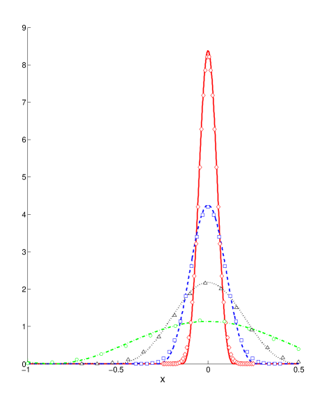
Figure 2: The Jackson kernel approximation $\delta^{(r)}_{\text{KPM}}$ to the Dirac delta function at $x^{*}=0$ for $r=8,16,32,64$. The corresponding scatterplots show the values of the Gaussian density function in (2.14) with $x^{*}=0$.

By construction, the function $\delta^{(r)}_{\text{KPM}}(x-x^{*})$ is nonnegative over $[-1,1]$ and we have the normalization $\int_{-1}^{1}\delta^{(r)}_{\text{KPM}}(x-x^{*})dx=\int_{-1}^{1}\delta_{x^{*}}(x)dx=1$ (cf. Section 2.2). Hence, it is a probability density function on $[-1,1]$ for the Lebesgue measure. It is convenient to consider the following univariate polynomial

$$h_{r}(x)=1+2\sum_{k=1}^{r}g^{r}_{k}T_{k}(x)T_{k}(x^{*}),$$ (2.15)

so that $\delta^{(r)}_{\text{KPM}}(x-x^{*})=\frac{1}{\pi\sqrt{1-x^{2}}}h_{r}(x).$ The following facts follow directly, which we will use below for the convergence analysis of the new bounds $f^{(r)}$.

Lemma 2.3

For any $r\in{\mathbb{N}}$ the polynomial $h_{r}$ from (2.15) is nonnegative over $[-1,1]$ and $\int_{-1}^{1}h_{r}(x)\frac{dx}{\pi\sqrt{1-x^{2}}}=1$. In other words, $h_{r}$ is a probability density function for the measure $\left(\pi\sqrt{1-x^{2}}\right)^{-1}dx$ on $[-1,1]$.

3 Convergence analysis

In this section we analyze the convergence rate of the new bounds $f^{(r)}$ and we show the result from Theorem 1.5. We will first consider the univariate case in Section 3.1 (see Theorem 3.3) and then the general multivariate case in Section 3.2 (see Theorem 3.6). As we will see, the polynomial $h_{r}$ arising from the Jackson kernel approximation of the Dirac delta function, introduced above in relation (2.15), will play a key role in the convergence analysis.

3.1 The univariate case

We consider a univariate polynomial $f$ and let $x^{*}$ be a global minimizer of $f$ in $[-1,1]$. As observed in Lemma 2.3 the polynomial $h_{r}$ from (2.15) is a density function for the measure $\frac{dx}{\pi\sqrt{1-x^{2}}}$. The key observation now is that the polynomial $h_{r}$ admits a Schmüdgen-type representation, of the form $\sigma(x)+\sigma_{1}(x)(1-x^{2})$ with $\sigma_{0},\sigma_{1}$ sums-of-squares polynomials, since it is non-negative over $[-1,1]$. This fact will allow us to use the polynomial $h_{r}$ to get feasible solutions for the program defining the bound $f^{(r)}$. It follows from the following classical result (see, e.g., [17]), that characterizes univariate polynomials that are nonnegative on $[-1,1]$. (Note that this is a strengthening of Schmüdgen’s theorem (Theorem 1.3) in the univariate case.)

Theorem 3.1 (Fekete, Markov-Lukàcz)

Let $p(x)$ be a univariate polynomial of degree $m$. Then $p(x)$ is nonnegative on the interval $[-1,1]$ if and only if it has the following representation:

$$p(x)=\sigma_{0}(x)+(1-x^{2})\sigma_{1}(x)$$

for some sum-of-squares polynomials $\sigma_{0}$ of degree $2\lceil m/2\rceil$ and $\sigma_{1}$ of degree $2\lceil m/2\rceil-2$.

We start with the following technical lemma.

Lemma 3.2

Let $f$ be a polynomial of degree $d$ written in the Chebyshev basis as $f=\sum_{k=0}^{d}f_{k}T_{k}$, let $x^{*}$ be a global minimizer of $f$ in $[-1,1]$, and let $h_{r}$ be the polynomial from (2.15). For any integer $r\geq d$ we have

$$\int_{-1}^{1}f(x)h_{r}(x)\frac{dx}{\pi\sqrt{1-x^{2}}}-f(x^{*})\leq\frac{C_{f}}{(r+2)^{2}},$$

where $C_{f}=(\sum_{k=1}^{d}|f_{k}|)\frac{C_{d}\pi^{2}}{2}$ and $C_{d}$ is the constant from Lemma 2.2.

Proof. As $f=\sum_{k=0}^{d}f_{k}T_{k}$ and $h_{r}=1+2\sum_{k=1}^{r}g_{k}^{r}T_{k}(x^{*})T_{k}$, we use the orthogonality relationships (2.6) to obtain

$$\int_{-1}^{1}f(x)h_{r}(x)\frac{dx}{\pi\sqrt{1-x^{2}}}=\sum_{k=0}^{d}f_{k}T_{k}(x^{*})g^{r}_{k}.$$ (3.1)

Combining with $f(x^{*})=\sum_{k=0}^{d}f_{k}T_{k}(x^{*})$ gives

$$\int_{-1}^{1}f(x)h_{r}(x)\frac{dx}{\pi\sqrt{1-x^{2}}}-f(x^{*})=\sum_{k=1}^{d}f_{k}T_{k}(x^{*})(g_{k}^{r}-1).$$ (3.2)

Now we use the upper bound on $g_{k}^{r}-1$ from Lemma 2.2 and the bound $|T_{k}(x^{*})|\leq 1$ to conclude the proof. $\Box$

We can now conclude the convergence analysis of the bounds $f^{(r)}$ in the univariate case.

Theorem 3.3

Let $f=\sum_{k=0}^{d}f_{k}T_{k}$ be a polynomial of degree $d$. For any integer $r\geq d$ we have

$$f^{(r)}-f_{\min}\leq\frac{C_{f}}{(r+1)^{2}},$$

where $C_{f}=(\sum_{k=1}^{d}|f_{k}|)\frac{C_{d}\pi^{2}}{2}$ and $C_{d}$ is the constant from Lemma 2.2.

Proof. Using the degree bounds in Theorem 3.1 for the sum-of-squares polynomials entering the decomposition of the polynomial $h_{r}$, we can conclude that for $r$ even, $h_{r}$ is feasible for the program defining the parameter $f^{(r)}$ and for $r$ odd, $h_{r}$ is feasible for the program defining the parameter $f^{(r+1)}$. Setting $C_{f}=(\sum_{k=1}^{d}|f_{k}|)\frac{C_{d}\pi^{2}}{2}$ and using Lemma 3.2, this implies: $f^{(r)}-f_{\min}\leq\frac{C_{f}}{(r+2)^{2}}$ for $r$ even, and $f^{(r)}-f_{\min}\leq\frac{C_{f}}{(r+1)^{2}}$ for odd $r$. The result of the theorem now follows. $\Box$

3.2 The multivariate case

We consider now a multivariate polynomial $f$ and we let $x^{*}=(x^{*}_{1},\dotsc,x^{*}_{n})\in[-1,1]^{n}$ denote a global minimizer of $f$ on $[-1,1]^{n}$, i.e., $f(x^{*})=f_{\min}$.

In order to obtain a feasible solution to the program defining the parameter $f^{(r)}$ we will consider products of the univariate polynomials $h_{r}$ from (2.15). Namely, given integers $r_{1},\ldots,r_{n}\in{\mathbb{N}}$ we define the $n$-tuple ${\underline{r}}=(r_{1},\ldots,r_{n})$ and the $n$-variate polynomial

$$H_{{\underline{r}}}(x_{1},\ldots,x_{n})=\prod_{i=1}^{n}h_{r_{i}}(x_{i}).$$ (3.3)

We group in the next lemma some properties of the polynomial $H_{{\underline{r}}}$.

Lemma 3.4

The polynomial $H_{\underline{r}}$ satisfies the following properties:

• $H_{{\underline{r}}}$ is non-negative on $[-1,1]^{n}$.

• $\int_{[-1,1]^{n}}H_{{\underline{r}}}(x)d\mu(x)=1$, where $d\mu$ is the measure from (1.7).

• $H_{{\underline{r}}}$ has a Schmüdgen-type representation of the form $H_{{\underline{r}}}(x)=\sum_{I\subseteq[n]}\sigma_{I}(x)\prod_{i\in I}(1-x_{i}^{2})$, where each $\sigma_{I}$ is a sum-of-squares polynomial of degree at most $2\sum_{i=1}^{n}\lceil r_{i}/2\rceil-2|I|$.

Proof. (i) and (ii) follow directly from the corresponding properties of the univariate polynomials $h_{r_{i}}$, and (iii) follows using Theorem 3.1 applied to the polynomials $h_{r_{i}}$. $\Box$

The next lemma is the analog of Lemma 3.2 for the multivariate case.

Lemma 3.5

Let $f$ be a multivariate polynomial of degree $d$, written in the basis of multivariate Chebyshev polynomials as $f=\sum_{\alpha\in{\mathbb{N}}^{n}:|\alpha|\leq d}f_{\alpha}T_{\alpha}$, and let $x^{*}$ be a global minimizer of $f$ in $[-1,1]^{n}$. Consider ${\underline{r}}=(r_{1},\ldots,r_{n})$, where each $r_{i}$ is an integer satisfying $r_{i}\geq d$, and the polynomial $H_{{\underline{r}}}$ from (3.3). We have

$$\int_{[-1,1]^{n}}f(x)H_{{\underline{r}}}(x)d\mu(x)-f(x^{*})\leq C_{f}\sum_{i=1}^{n}\frac{1}{(r_{i}+2)^{2}},$$

where $C_{f}=(\sum_{\alpha:|\alpha|\leq d}|f_{\alpha}|)\frac{C_{d}\pi^{2}}{2}$ and $C_{d}$ is the constant from Lemma 2.2.

Proof. As $f=\sum_{\alpha:|\alpha|\leq d}f_{\alpha}T_{\alpha}$ and $H_{{\underline{r}}}=\prod_{i=1}^{n}h_{r_{i}}(x_{i})=\prod_{i=1}^{n}(1+2\sum_{k_{i}=1}^{r_{i}}g_{k_{i}}^{r_{i}}T_{k_{i}}(x_{i})T_{k_{i}}(x_{i}^{*}))$, we can use the orthogonality relationships (2.9) among the multivariate Chebyshev polynomials to derive

$$\int_{[-1,1]^{n}}f(x)H_{{\underline{r}}}(x)d\mu(x)=\sum_{\alpha:|\alpha|\leq d}f_{\alpha}T_{\alpha}(x^{*})\prod_{i=1}^{n}g_{\alpha_{i}}^{r_{i}}.$$

Combining this with $f(x^{*})=\sum_{\alpha:|\alpha|\leq d}f_{\alpha}T_{\alpha}(x^{*})$ gives:

$$\int_{[-1,1]^{n}}f(x)H_{{\underline{r}}}(x)d\mu(x)-f(x^{*})=\sum_{\alpha:|\alpha|\leq d}f_{\alpha}T_{\alpha}(x^{*})(\prod_{i=1}^{n}g_{\alpha_{i}}^{r_{i}}-1).$$

Using the identity: $\prod_{i=1}^{n}g_{\alpha_{i}}^{r_{i}}-1=\sum_{j=1}^{n}(g^{r_{j}}_{\alpha_{j}}-1)\prod_{k=j+1}^{n}g^{r_{k}}_{\alpha_{k}}$ and the fact that $|g^{r_{k}}_{\alpha_{k}}|\leq 1$, we get $|\prod_{i=1}^{n}g_{\alpha_{i}}^{r_{i}}-1|\leq\sum_{j=1}^{n}|g^{r_{j}}_{\alpha_{j}}-1|$. Now use $|T_{\alpha}(x^{*})|\leq 1$ and the bound from Lemma 2.2 for each $|1-g_{\alpha_{j}}^{r_{j}}|$ to conclude the proof. $\Box$

We can now show our main result, which implies Theorem 1.5.

Theorem 3.6

Let $f=\sum_{\alpha:|\alpha|\leq d}f_{\alpha}T_{\alpha}$ be an $n$-variate polynomial of degree $d$. For any integer $r\geq n(d+2)$, we have

$$f^{(r)}-f_{\min}\leq\frac{C_{f}n^{3}}{(r+1)^{2}},$$

where $C_{f}=(\sum_{\alpha:|\alpha|\leq d}|f_{\alpha}|)\frac{C_{d}\pi^{2}}{2}$ and $C_{d}$ is the constant from Lemma 2.2.

Proof. Write $r-n=sn+n_{0}$, where $s,n_{0}\in{\mathbb{N}}$ and $0\leq n_{0}<n$, and define the $n$-tuple ${\underline{r}}=(r_{1},\ldots,r_{n})$, setting $r_{i}=s+1$ for $1\leq i\leq n_{0}$ and $r_{i}=s$ for $n_{0}+1\leq i\leq n$, so that $r-n=r_{1}+\ldots+r_{n}$. Note that the condition $r\geq n(d+2)$ implies $s\geq d$ and thus $r_{i}\geq d$ for all $i$. Moreover, we have: $2\sum_{i=1}^{n}\lceil r_{i}/2\rceil=2n_{0}\lceil(s+1)/2\rceil+2(n-n_{0})\lceil s/2\rceil$, which is equal to $r-n+n_{0}$ for even $s$ and to $r-n_{0}$ for odd $s$ and thus always at most $r$. Hence the polynomial $H_{{\underline{r}}}$ from (3.3) has degree at most $r$. By Lemma 3.4(ii), (iii), it follows that the polynomial $H_{{\underline{r}}}$ is feasible for the program defining the parameter $f^{(r)}$. By Lemma 3.5 this implies that

$$f^{(r)}-f_{\min}\leq\int_{[-1,1]^{n}}f(x)H_{{\underline{r}}}(x)d\mu(x)-f(x^{*})\leq C_{f}\sum_{i=1}^{n}\frac{1}{(r_{i}+2)^{2}}.$$

Finally, $\sum_{i=1}^{n}\frac{1}{(r_{i}+2)^{2}}=\frac{n_{0}}{(s+3)^{2}}+\frac{n-n_{0}}{(s+2)^{2}}\leq\frac{n}{(s+2)^{2}}=\frac{n^{3}}{(r+n-n_{0})^{2}}\leq\frac{n^{3}}{(r+1)^{2}}$, since $n_{0}\leq n-1$. $\Box$

4 Computing the parameter $f^{(r)}$ as a generalized eigenvalue problem

As the parameter $f^{(r)}$ is defined in terms of sum-of-squares polynomials (cf. Definition 1.4), it can be computed by means of a semidefinite program. As we now observe, as the program (1.8) has only one affine constraint, $f^{(r)}$ can in fact be computed in a cheaper way as a generalized eigenvalue problem.

Using the inner product from (2.5), the parameter $f^{(r)}$ can be rewritten as

$$\begin{array}[]{ll}\displaystyle f^{(r)}=\min_{h\in{\mathbb{R}}[x]}\langle f,h\rangle\ \text{ such that }&\langle h,T_{0}\rangle=1,\ h(x)=\sum_{I\subseteq[n]}\sigma_{I}(x)\prod_{i\in I}(1-x_{i}^{2}),\\ &\sigma_{I}\in\Sigma[x],\ \deg(\sigma_{I})\leq r-2|I|\ \;\forall I\subseteq[n].\end{array}$$ (4.1)

For convenience we use below the following notation. For a set $I\subseteq[n]$ and an integer $r\in{\mathbb{N}}$ we let $\Lambda^{I}_{r}$ denote the set of sequences $\beta\in{\mathbb{N}}^{n}$ with $|\beta|\leq\lfloor\frac{r-2|I|}{2}\rfloor$. As is well known one can express the condition that $\sigma_{I}$ is a sum-of-squares polynomial, i.e., of the form $\sum_{k}p_{k}(x)^{2}$ for some $p_{k}\in{\mathbb{R}}[x]$, as a semidefinite program. More precisely, using the Chebyshev basis to express the polynomials $p_{k}$, we obtain that $\sigma_{I}$ is a sum-of-squares polynomial if and only if there exists a matrix variable $M^{I}$ indexed by $\Lambda^{I}_{r}$, which is positive semidefinite and satisfies

$$\sigma_{I}=\sum_{\beta,\gamma\in\Lambda^{I}_{r}}M^{I}_{\beta,\gamma}T_{\beta}T_{\gamma}.$$ (4.2)

For each $I\subseteq[n]$, we introduce the following matrices $A^{I}$ and $B^{I}$, which are also indexed by the set $\Lambda^{I}_{r}$ and, for $\beta,\gamma\in\Lambda^{I}_{r}$, with entries

$$\begin{array}[]{l}\displaystyle A^{I}_{\beta,\gamma}=\langle f,T_{\beta}T_{\gamma}\prod_{i\in I}(1-x_{i}^{2})\rangle,\\ \displaystyle B^{I}_{\beta,\gamma}=\langle T_{0},T_{\beta}T_{\gamma}\prod_{i\in I}(1-x_{i}^{2})\rangle.\end{array}$$ (4.3)

We will indicate in the appendix how to compute the matrices $A^{I}$ and $B^{I}$.

We can now reformulate the parameter $f^{(r)}$ as follows.

Lemma 4.1

Let $A^{I}$ and $B^{I}$ be the matrices defined as in (4.3) for each $I\subseteq[n]$. Then the parameter $f^{(r)}$ can be reformulated using the following semidefinite program in the matrix variables $M^{I}$ ($I\subseteq[n]$):

$$f^{(r)}=\min_{M^{I}:I\subseteq[n]}\ \sum_{I\subseteq[n]}{\rm Tr\,}(A^{I}M^{I})\ \text{ such that }\ M^{I}\succeq 0\ \forall I\subseteq[n],\ \sum_{I\subseteq[n]}{\rm Tr\,}(B^{I}M^{I})=1.$$ (4.4)

Proof. Using relation (4.2) we can express the polynomial variable $h$ in (4.1) in terms of the matrix variables $M^{I}$ and obtain

$$h=\sum_{I\subseteq[n]}\sum_{\beta,\gamma\in\Lambda^{I}_{r}}M^{I}_{\beta,\gamma}T_{\beta}T_{\gamma}\prod_{i\in I}(1-x_{i})^{2}.$$

First this permits us to reformulate the objective function $\langle f,h\rangle$ in terms of the matrix variables $M^{I}$ in the following way:

$$\begin{array}[]{ll}\langle f,h\rangle&=\sum_{I}\sum_{\beta,\gamma}M^{I}_{\beta,\gamma}\langle f,T_{\beta}T_{\gamma}\prod_{i\in I}(1-x_{i}^{2})\rangle\\ &=\sum_{I}\sum_{\beta,\gamma}M^{I}_{\beta,\gamma}A^{I}_{\beta,\gamma}\\ &=\sum_{I}{\rm Tr\,}(A^{I}M^{I}).\end{array}$$

Second we can reformulate the constraint $\langle T_{0},h\rangle=1$ using

$$\begin{array}[]{ll}\langle T_{0},h\rangle&=\sum_{I}\sum_{\beta,\gamma}M^{I}_{\beta,\gamma}\langle T_{0},T_{\beta}T_{\gamma}\prod_{i\in I}(1-x_{i}^{2})\rangle\\ &=\sum_{I}\sum_{\beta,\gamma}M^{I}_{\beta,\gamma}B^{I}_{\beta,\gamma}\\ &=\sum_{I}{\rm Tr\,}(B^{I}M^{I}).\end{array}$$

From this follows that the program (4.1) is indeed equivalent to the program (4.4). $\Box$

The program (4.4) is a semidefinite program with only one constraint. Hence, as we show next, it is equivalent to a generalized eigenvalue problem.

Theorem 4.2

For $I\subseteq[n]$ let $A^{I}$ and $B^{I}$ be the matrices from (4.3) and define the parameter

$$\lambda^{(I)}=\max\left\{\lambda\;|\;A^{I}-\lambda B^{I}\succeq 0\right\}=\min\left\{\lambda\;|\;A^{I}x=\lambda B^{I}x\mbox{ for some non-zero vector $x$}\right\}.$$

One then has $f^{(r)}=\min_{I\subseteq[n]}\lambda^{(I)}$.

Proof. The dual semidefinite program of the program (4.4) is given by

$$\sup\left\{\lambda\;|\;A^{I}-\lambda B^{I}\succeq 0\;\;\;\forall I\subseteq[n]\right\}.$$ (4.5)

We first show that the primal problem (4.4) is strictly feasible. To see this it suffices to show that ${\rm Tr\,}(B^{I})>0$, since then one may set $M_{I}$ equal to a suitable multiple of the identity matrix and thus one gets a strictly feasible solution to (4.4). Indeed, the matrix $B^{I}$ is positive semidefinite since, for any scalars $g_{\beta}$,

$$\sum_{\beta,\gamma}g_{\beta}g_{\gamma}B^{I}_{\beta\gamma}=\int_{[-1,1]^{n}}\Bigl{(}\sum_{\beta}g_{\beta}T_{\beta}\Bigr{)}^{2}\prod_{i\in I}(1-x_{i}^{2})d\mu(x)\geq 0.$$

Thus ${\rm Tr\,}(B^{I})\geq 0$ and, moreover, ${\rm Tr\,}(B^{I})>0$ since $B^{I}$ is nonzero.

Moreover, the dual problem (4.5) is also feasible, since $\lambda=f_{\min}$ is a feasible solution. This follows from the fact that the polynomial $f-f_{\min}$ is nonnegative over $[-1,1]^{n}$, which implies that the matrix $A^{I}-f_{\min}B^{I}$ is positive semidefinite. Indeed, using the same argument as above for showing that $B^{I}\succeq 0$, we have

$$\sum_{\beta,\gamma}g_{\beta}g_{\gamma}(A^{I}-f_{\min}B^{I})_{\beta,\gamma}=\int_{[-1,1]^{n}}(f(x)-f_{\min})\Bigl{(}\sum_{\beta}g_{\beta}T_{\beta}\Bigr{)}^{2}\prod_{i\in I}(1-x_{i}^{2})d\mu(x)\geq 0.$$

Since the primal problem is strictly feasible and the dual problem is feasible, there is no duality gap and the dual problem attains its supremum. The result follows. $\Box$

5 Numerical examples

We examine the polynomial test functions which were also used in [4] and [3], and are described in the appendix to this paper.

The numerical examples given here only serve to illustrate the observed convergence behavior of the sequence $f^{(r)}$ as compared to the theoretical convergence rate. In particular, the computational demands for computing $f^{(r)}$ for large $r$ are such that it cannot compete in practice with the known iterative methods referenced in the introduction.

For the polynomial test functions we list in (Table 1) the values of $f^{(r)}$ for even $r$ up to $r=48$, obtained by solving the generalized eigenvalue problem in Theorem 4.2 using the eig function of Matlab. Recall that for step $r$ of the hierarchy the polynomial density function $h$ is of Schmüdgen-type and has degree $r$.

For the examples listed the computational time is negligible, and therefore not listed; recall that the computation of $f^{(r)}$ for even $n$ requires the solution of $2^{n}$ generalized eigenvalue problems indexed by subsets $I\subset[n]$, where the order of the matrices equals $\binom{n+{\lfloor r/2-|I|\rfloor}}{n}$; cf. Theorem 4.2.

Table 1: The upper bounds $f^{(r)}$ for the test functions.

$r$	Booth	Matyas	Motzkin	Three-Hump	Styblinski-Tang		Rosenbrock
					$n=2$	$n=3$	$n=2$	$n=3$
6	145.3633	4.1844	1.1002	24.6561	-27.4061		157.7604
8	118.0554	3.9308	0.8764	15.5022	-34.5465	-40.1625	96.8502	318.0367
10	91.6631	3.8589	0.8306	9.9919	-40.0362	-47.6759	68.4239	245.9925
12	71.1906	3.8076	0.8098	6.5364	-47.4208	-55.4061	51.7554	187.2490
14	57.3843	3.0414	0.7309	4.5538	-51.2011	-64.0426	39.0613	142.8774
16	47.6354	2.4828	0.6949	3.3453	-56.0904	-70.2894	30.3855	111.0703
18	40.3097	2.0637	0.5706	2.5814	-58.8010	-76.0311	24.0043	88.3594
20	34.5306	1.7417	0.5221	2.0755	-61.8751	-80.5870	19.5646	71.5983
22	28.9754	1.4891	0.4825	1.7242	-63.9161	-85.4149	16.2071	59.0816
24	24.6380	1.2874	0.4081	1.4716	-65.5717	-88.5665	13.6595	49.5002
26	21.3151	1.1239	0.3830	1.2830	-67.2790		11.6835
28	18.7250	0.9896	0.3457	1.1375	-68.2078		10.1194
30	16.6595	0.8779	0.3016	1.0216	-69.5141		8.8667
32	14.9582	0.7840	0.2866	0.9263	-70.3399		7.8468
34	13.5114	0.7044	0.2590	0.8456	-71.0821		7.0070
36	12.2479	0.6363	0.2306	0.7752	-71.8284		6.3083
38	11.0441	0.5776	0.2215	0.7129	-72.2581		5.7198
40	10.0214	0.5266	0.2005	0.6571	-72.8953		5.2215
42	9.1504	0.4821	0.1815	0.6070	-73.3011		4.7941
44	8.4017	0.4430	0.1754	0.5622	-73.6811		4.4266
46	7.7490	0.4084	0.1597	0.5220	-74.0761		4.1070
48	7.1710	0.3778	0.1462	0.4860	-74.3070		3.8283

We note that the observed rate of convergence seems in line with the $O(1/r^{2})$ error bound.

As a second numerical experiment, we compare (see Table 2) the upper bound $f^{(r)}$ to the upper bound $\underline{f}_{\mathbf{K}}^{(r)}$ defined in (1.2). Recall that the bound $\underline{f}_{\mathbf{K}}^{(r)}$ corresponds to using sum-of-squares density functions of degree at most $r$ and the Lebesgue measure. As shown in [4], the computation of $\underline{f}_{\mathbf{K}}^{(r)}$ may be done by solving a single generalized eigenvalue problem with matrices of order $\binom{n+{\lfloor r/2-|I|\rfloor}}{n}$. Thus the computation of $\underline{f}_{\mathbf{K}}^{(r)}$ is significantly cheaper than that of $f^{(r)}$.

Table 2: Comparison of the upper bounds $f^{(r)}$ and $\underline{f}_{\mathbf{K}}^{(r)}$ for Booth, Matyas, Three–Hump Camel, and Motzkin functions.

$r$	Booth function		Matyas function		Three–Hump Camel function		Motzkin polynomial
	$\underline{f}_{\mathbf{K}}^{(r)}$	$f^{(r)}$	$\underline{f}_{\mathbf{K}}^{(r)}$	$f^{(r)}$	$\underline{f}_{\mathbf{K}}^{(r)}$	$f^{(r)}$	$\underline{f}_{\mathbf{K}}^{(r)}$	$f^{(r)}$
$6$	118.383	145.3633	4.2817	4.1844	29.0005	24.6561	1.0614	1.1002
$8$	97.6473	118.0554	3.8942	3.9308	9.5806	15.5022	0.8294	0.8764
$10$	69.8174	91.6631	3.6894	3.8589	9.5806	9.9919	0.8010	0.8306
$12$	63.5454	71.1906	2.9956	3.8076	4.4398	6.5364	0.8010	0.8098
$14$	47.0467	57.3843	2.5469	3.0414	4.4398	4.5538	0.7088	0.7309
$16$	41.6727	47.6354	2.0430	2.4828	2.5503	3.3453	0.5655	0.6949
$18$	34.2140	40.3097	1.8335	2.0637	2.5503	2.5814	0.5655	0.5706
$20$	28.7248	34.5306	1.4784	1.7417	1.7127	2.0755	0.5078	0.5221
$22$	25.6050	28.9754	1.3764	1.4891	1.7127	1.7242	0.4060	0.4825
$24$	21.1869	24.6380	1.1178	1.2874	1.2775	1.4716	0.4060	0.4081
$26$	19.5588	21.3151	1.0686	1.1239	1.2775	1.2830	0.3759	0.3830
$28$	16.5854	18.7250	0.8742	0.9896	1.0185	1.1375	0.3004	0.3457
$30$	15.2815	16.6595	0.8524	0.8779	1.0185	1.0216	0.3004	0.3016
$32$	13.4626	14.9582	0.7020	0.7840	0.8434	0.9263	0.2819	0.2866
$34$	12.2075	13.5114	0.6952	0.7044	0.8434	0.8456	0.2300	0.2590
$36$	11.0959	12.2479	0.5760	0.6363	0.7113	0.7752	0.2300	0.2306
$38$	9.9938	11.0441	0.5760	0.5776	0.7113	0.7129	0.2185	0.2215
$40$	9.2373	10.0214	0.4815	0.5266	0.6064	0.6571	0.1817	0.2005

It is interesting to note that, in almost all cases, $f^{(r)}>\underline{f}_{\mathbf{K}}^{(r)}$. Thus even though the measure $d\mu(x)$ and the Schmüdgen-type densities are useful in getting improved error bounds, they mostly do not lead to improved upper bounds for these examples. This also suggests that it might be possible to improve the error result $\underline{f}_{\mathbf{K}}^{(r)}-f_{\min}=O(1/\sqrt{r})$ in [4], at least for the case ${\mathbf{K}}=[-1,1]^{n}$. To illustrate this effect we graphically represented the results of Table 2 in Figure 3. Note that the bound $\frac{C_{f}n^{3}}{(r+1)^{2}}$ of Theorem 3.6 would lie far above these graphs. To give an idea for the value of the constants $C_{f}$ we calculated them for the Booth, Matyas, Three-Hump Camel,and Motzkin functions: $C_{\text{Booth}}\approx 2.6\cdot 10^{5},\ C_{\text{Matyas}}\approx 9.9\cdot 10^{3},\ C_{\text{ThreeHump}}\approx 3.5\cdot 10^{7}$ and $C_{\text{Motzkin}}\approx 1.1\cdot 10^{5}$.

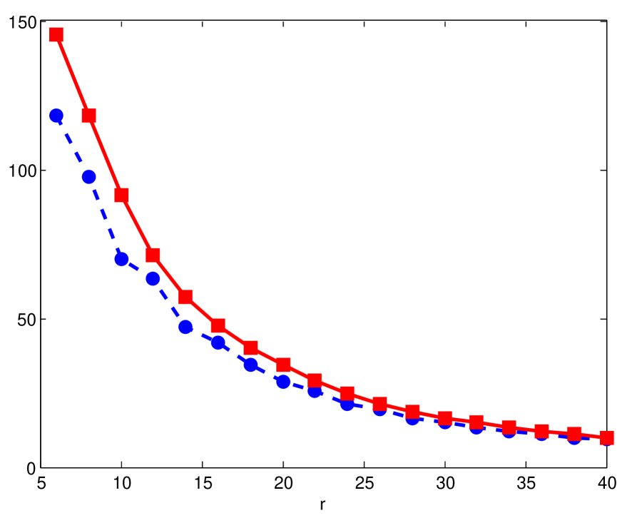
(a) Booth function

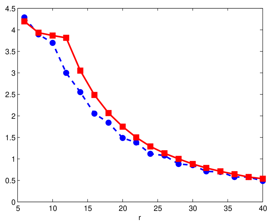
(b) Matyas function

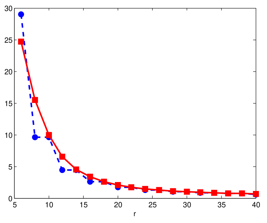
(c) Three-Hump Camel function

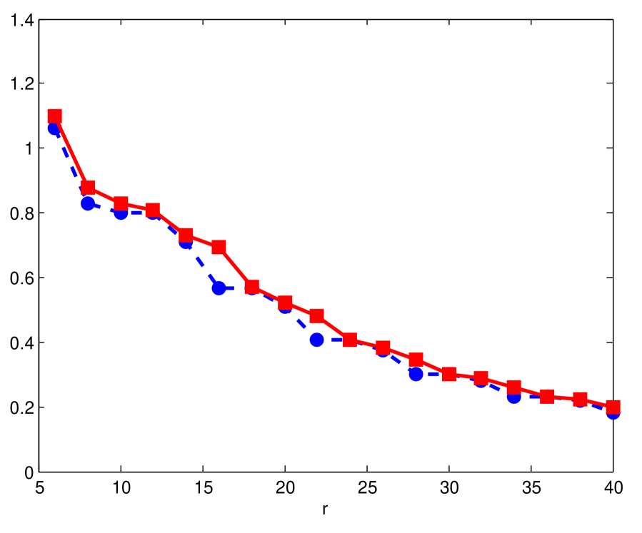
(d) Motzkin polynomial

Figure 3: Graphical representation of Table 2 to illustrate the comparison of the upper bounds $\underline{f}_{\mathbf{K}}^{(r)}$ and $f^{(r)}$. The values $\underline{f}_{\mathbf{K}}^{(r)}$ are marked with circles connected by a dashed line and $f^{(r)}$ with squares connected by a solid line.

Finally, it is shown in [4] that one may obtain feasible points corresponding to bounds like $f^{(r)}$ through sampling from the probability distribution defined by the optimal density function. In particular, one may use the method of conditional distributions (see e.g., [12, Section 8.5.1]). For $\mathbf{K}=[0,1]^{n}$, the procedure is described in detail in [4, Section 3].

Appendix

A. Proof of Lemma 2.1

We give here a proof of Lemma 2.1, which we repeat for convenience.

Lemma 2.1 For any fixed integer $k>1$, one has

$$\max_{0\leq i\leq k-1}|u_{i}^{(k)}|\leq\max_{0\leq i\leq k}|t_{i}^{(k)}|=2^{k-1-2\psi(k)}\frac{k(k-\psi(k)-1)!}{\psi(k)!(k-2\psi(k))!},$$ (2.7)

where $\psi(k)=0$ for $k\leq 4$ and $\psi(k)=\left\lceil\frac{1}{8}\left(4k-5-\sqrt{8k^{2}-7}\right)\right\rceil$ for $k\geq 4$. Moreover, the right-hand side of the equation increases monotonically with increasing $k$.

Proof. We recall the representation of the Chebyshev polynomials in the monomial basis:

$$T_{k}(x) =\sum_{i=0}^{k}t_{i}^{(k)}x^{i}=\frac{k}{2}\sum_{m=0}^{\lfloor\frac{k}{2}\rfloor}(-1)^{m}\frac{(k-m-1)!}{m!(k-2m)!}(2x)^{k-2m}, k>0,$$

$$U_{k-1}(x) =\sum_{i=0}^{k-1}u_{i}^{(k)}x^{i}=\sum_{m=0}^{\lfloor\frac{k-1}{2}\rfloor}(-1)^{m}\frac{(k-m-1)!}{m!(k-1-2m)!}(2x)^{k-1-2m}, k>1.$$

So, concretely, the coefficients are given by

$$t_{k-2m}^{(k)} =(-1)^{m}\cdot 2^{k-1-2m}\cdot\frac{k(k-m-1)!}{m!(k-2m)!}, k>0,\ 0\leq m\leq\left\lfloor\frac{k}{2}\right\rfloor,$$

$$u_{k-1-2m}^{(k)} =(-1)^{m}\cdot 2^{k-1-2m}\cdot\frac{(k-m-1)!}{m!(k-1-2m)!}, k>1,\ 0\leq m\leq\left\lfloor\frac{k-1}{2}\right\rfloor.$$

It follows directly that $t_{k-2m}^{(k)}=\frac{k}{k-2m}u_{k-1-2m}^{(k)}$ and thus $|t_{k-2m}^{(k)}|>|u_{k-1-2m}^{(k)}|$ for $m<\frac{k}{2}$ and all $k>1$ which implies the inequality on the left-hand side of (2.7).

Now we show that the value of $\max_{0\leq m\leq\left\lfloor\frac{k}{2}\right\rfloor}|t_{k-2m}^{(k)}|$ is attained for $m=\psi(k)$. For this we examine the quotient

$$\frac{|t_{k-2(m+1)}^{(k)}|}{|t_{k-2m}^{(k)}|}=\frac{(k-2m)(k-2m-1)}{4(m+1)(k-m-1)}\\ =\frac{k^{2}-4mk+4m^{2}+2m-k}{4mk-4m^{2}-8m+4k-4}.$$ (A.1)

Observe that this quotient is at most 1 if and only if $m_{1}\leq m\leq m_{2}$, where we set $m_{1}=\frac{1}{8}\left(4k-5-\sqrt{8k^{2}-7}\right)$ and $m_{2}=\frac{1}{8}\left(4k-5+\sqrt{8k^{2}-7}\right)$. Hence the function $m\mapsto|t_{k-2m}^{(k)}|$ is monotone increasing for $m\leq m_{1}$ and monotone decreasing for $m_{1}\leq m\leq m_{2}$. Moreover, as $\lfloor m_{1}\rfloor\leq m_{1}$, we deduce that $|t^{(k)}_{k-2\lceil m_{1}\rceil}|\geq|t^{(k)}_{k-2\lfloor m_{1}\rfloor}|$. Observe furthermore that $m_{1}\geq 0$ if and only if $k\geq 4$, and $m_{2}\geq\frac{k}{2}$ for all $k>1$.

Therefore, in the case $k\geq 4$, $\max_{0\leq m\leq\left\lfloor\frac{k}{2}\right\rfloor}|t_{k-2m}^{(k)}|$ is attained at $\lceil m_{1}\rceil=\psi(k),$ and thus it is equal to $|t^{(k)}_{k-2\psi(k)}|$. In the case $1<k\leq 4$, $\max_{0\leq m\leq\left\lfloor\frac{k}{2}\right\rfloor}|t_{k-2m}^{(k)}|$ is attained at $m=0$, and thus it is equal to $|t^{(k)}_{k}|=2^{k-1}.$

Finally we show that the rightmost term of (2.7) increases monotonically with $k$. We show the inequality: $|t^{(k)}_{k-2\psi(k)}|\leq|t^{(k+1)}_{k+1-2\psi(k+1)}|$ for $k\geq 4$. For this we consider again the sequence of Chebyshev coefficients, but this time we are interested in the behavior for increasing $k$, i.e., in the map $k\mapsto|t_{k-2m}^{(k)}|$. So, for fixed $m$, we consider the quotient

$$\frac{|t_{k+1-2m}^{(k+1)}|}{|t_{k-2m}^{(k)}|}=\frac{2^{k-2m}(k+1)(k-m)!\,m!\,(k-2m)!}{2^{k-1-2m}k(k-m-1)!\,m!\,(k+1-2m)!}=2\cdot\frac{k+1}{k}\cdot\frac{k-m}{k+1-2m},$$

which is equal to 2 if $m=0$, and at least 1 if $m>0$ since every factor is at least 1. Thus, for $m=\psi(k)$, we obtain

$$|t^{(k)}_{k-2\psi(k)}|\leq|t^{(k+1)}_{k+1-2\psi(k)}|.$$ (A.2)

Consider the map $\phi\colon[4,\infty)\to\mathbb{R},\ k\mapsto\phi(k)=\frac{1}{8}\left(4k-5-\sqrt{8k^{2}-7}\right)$, so that $\psi(k)=\lceil\phi(k)\rceil$. The map $\phi$ is monotone increasing, since its derivative $\phi^{\prime}(k)=\frac{1}{8}\left(4-\frac{16k}{2\sqrt{8k^{2}-7}}\right)=\frac{\sqrt{8k^{2}-7}-2k}{2\sqrt{8k^{2}-7}}$ is positive for all $k\geq 4$. Hence, we have: $\psi(k)\leq\psi(k+1)$. Then, in view of (A.1) (and the comment thereafter), we have $|t^{(k+1)}_{k+1-2m}|\leq|t^{(k+1)}_{k+1-2(m+1)}|\ \text{ if }m\leq\psi(k+1),$ and thus

$$|t^{(k+1)}_{k+1-2\psi(k)}|\leq|t^{(k+1)}_{k+1-2\psi(k+1)}|.$$ (A.3)

Combining (A.2) and (A.3), we obtain the desired inequality: $|t^{(k)}_{k-2\psi(k)}|\leq|t^{(k+1)}_{k+1-2\psi(k+1)}|.$ $\Box$

B. Useful identities for the Chebychev polynomials

Recall the notation $d\mu(x)$ to denote the Lebesgue measure with the function $\prod_{i=1}^{n}\left(\pi\sqrt{1-x_{i}^{2}}\right)^{-1}$ as density function. In order to compute the matrices $A^{I}$ and $B^{I}$ we need to evaluate the following integrals:

$$\langle T^{\alpha},T^{\beta}T^{\gamma}\prod_{i\in I}(1-x_{i}^{2})\rangle=\prod_{i\in I}\int_{-1}^{1}T_{\alpha_{i}}(x_{i})T_{\beta_{i}}(x_{i})T_{\gamma_{i}}(x_{i})(1-x_{i}^{2})d\mu(x_{i})\cdot\prod_{i\not\in I}\int_{-1}^{1}T_{\alpha_{i}}(x_{i})T_{\beta_{i}}(x_{i})T_{\gamma_{i}}(x_{i})d\mu(x_{i}).$$

Thus we can now assume that we are in the univariate case. Suppose we are given integers $a,b,c\geq 0$ and the goal is to evaluate the integrals

$$\int_{-1}^{1}T_{a}(x)T_{b}(x)T_{c}(x)d\mu(x)\ \text{ and }\ \int_{-1}^{1}T_{a}(x)T_{b}(x)T_{c}(x)(1-x^{2})d\mu(x).$$

We use the following identities for the (univariate) Chebyshev polynomials:

$$T_{a}T_{b}=\tfrac{1}{2}(T_{a+b}+T_{|a-b|}),\ T_{a}T_{b}T_{c}=\tfrac{1}{4}(T_{a+b+c}+T_{|a+b-c|}+T_{|a-b|+c}+T_{||a-b|-c|}),$$

so that

$$T_{a}T_{b}T_{c}T_{2} = \tfrac{1}{8}(T_{a+b+c+2}+T_{|a+b+c-2|}+T_{|a+b-c|+2}+T_{||a+b-c|-2|}$$

$$+T_{|a-b|+c+2}+T_{||a-b|+c-2|}+T_{||a-b|-c|+2}+T_{|||a-b|-c|-2|}).$$

Using the orthogonality relation $\int_{-1}^{1}T_{a}d\mu(x)=\delta_{0,a}$, we obtain that

$$\int_{-1}^{1}T_{a}T_{b}T_{c}d\mu(x)=\tfrac{1}{4}(\delta_{0,a+b+c}+\delta_{0,a+b-c}+\delta_{0,|a-b|+c}+\delta_{0,|a-b|-c}).$$

Moreover, using the fact that $1-x^{2}=(1-T_{2})/2$, we get

$$\int_{-1}^{1}T_{a}T_{b}T_{c}(1-x^{2})d\mu(x)=\frac{1}{2}\int_{-1}^{1}T_{a}T_{b}T_{c}(1-T_{2})d\mu(x)=\frac{1}{2}\int_{-1}^{1}T_{a}T_{b}T_{c}d\mu(x)-\frac{1}{2}\int_{-1}^{1}T_{a}T_{b}T_{c}T_{2}d\mu(x),$$

and thus

$$\int_{-1}^{1}T_{a}T_{b}T_{c}(1-x^{2})d\mu(x) = \tfrac{1}{8}(\delta_{0,a+b+c}+\delta_{0,a+b-c}+\delta_{0,|a-b|+c}+\delta_{0,|a-b|-c})$$

$$-\tfrac{1}{16}(\delta_{0,a+b+c-2}+\delta_{0,|a+b-c|-2}+\delta_{0,|a-b|+c-2}+\delta_{0,||a-b|-c|-2}).$$

C. Test functions

Booth function

$n=2$, $f_{\min}=f(0.1,0.3)=0$, $f([-1,1]^{2})\approx[0,2\,500]$

$$f(x)=(10x_{1}+20x_{2}-7)^{2}+(20x_{1}+10x_{2}-5)^{2}\\ =250(T_{2}(x_{1})+T_{2}(x_{2}))+800\,T_{1}(x_{1})T_{1}(x_{2})-340\,T_{1}(x_{1})-380\,T_{1}(x_{2})+574.$$

Matyas function

$n=2$, $f_{\min}=f(0,0)=0$, $f([-1,1]^{2})\approx[0,100]$

$$f(x)=26(x_{1}^{2}+x_{2}^{2})-48x_{1}x_{2}=13(T_{2}(x_{1})+T_{2}(x_{2}))-48T_{1}(x_{1})T_{1}(x_{2})+26.$$

Motzkin polynomial

$n=2$, $f_{\min}=f(\pm\tfrac{1}{2},\pm\tfrac{1}{2})=0$, $f([-1,1]^{2})\approx[0,80]$

$$f(x)=64(x_{1}^{4}x_{2}^{2}+x_{1}^{2}x_{2}^{4})-48x_{1}^{2}x_{2}^{2}+1=4(T_{4}(x_{1})+T_{4}(x_{1})T_{2}(x_{2})\\ +T_{2}(x_{1})T_{4}(x_{2})+T_{4}(x_{2}))+20\,T_{2}(x_{1})T_{2}(x_{2})+16\,(T_{2}(x_{1})+T_{2}(x_{2}))+13.$$

Three-Hump Camel function

$n=2$, $f_{\min}=f(0,0)=0$, $f([-1,1]^{2})\approx[0,2\,000]$

$$f(x)=\frac{5^{6}}{6}x_{1}^{6}-5^{4}\cdot 1.05x_{1}^{4}+50x_{1}^{2}+25x_{1}x_{2}+25x_{2}^{2}\\ =\frac{5^{6}}{192}\,T_{6}(x_{1})+\frac{1625}{4}\,T_{4}(x_{1})+\tfrac{58725}{64}\,T_{2}(x_{1})+25\,T_{1}(x_{1})T_{1}(x_{2})+12.5\,T_{2}(x_{2})+\tfrac{14525}{24}.$$

Styblinski-Tang function

$n=2,\,3$, $f_{\min}=-39.17\cdot n$,$f([-1,1]^{2}\approx[-70,200]$

$$f(x)=\sum_{j=1}^{n}312.5x_{j}^{4}-200x_{j}^{2}+12.5x_{j}=\sum_{j=1}^{n}\left(\frac{625}{16}\,T_{4}(x_{j})+\frac{225}{4}\,T_{2}(x_{j})+\frac{25}{2}\,T_{1}(x_{j})+\frac{275}{16}\right).$$

Rosenbrock function

$n=2,\ 3$, $f_{\min}=0$, $f([-1,1]^{2})\approx[0,4\,000]$

$$f(x)=\sum_{j=1}^{n-1}100(2.048\cdot x_{j+1}-2.048^{2}\cdot x_{j}^{2})^{2}+(2.048\cdot x_{j}-1)^{2}\\ =\sum_{j=1}^{n-1}\left[12.5\cdot 2.048^{4}\,T_{4}(x_{j})-100\cdot 2.048^{3}\,T_{2}(x_{j})T_{1}(x_{j+1})+(0.5+50\cdot 2.048^{2})2.048^{2}\,T_{2}(x_{j})\right.\\ \left.+50\cdot 2.048^{2}\,T_{2}(x_{j+1})-4.096\,T_{1}(x_{j})-100\cdot 2.048^{3}\,T_{1}(x_{j+1})+1+2.048^{2}(37.5\cdot 2.048^{2}+50.5)\right].$$

References

- [1] D.P. Bertsekas, Constrained Optimization and Lagrange Multiplier Methods, Athena Scientific, Belmont, MA (1996)
- [2] M. Abramowitz, I.A. Stegun (eds.). Handbook of Mathematical Functions with formulas, graphs, and mathematical tables, 10th ed., Applied Mathematics Series 55, New York (1972)
- [3] E. de Klerk, J.B. Lasserre, M. Laurent, Z. Sun. Bound-constrained polynomial optimization using only elementary calculations, arxiv: 1507.04404 (2015)
- [4] E. de Klerk, M. Laurent, Z. Sun. Convergence analysis for Lasserre’s measure-based hierarchy of upper bounds for polynomial optimization, arXiv: 1411.6867 (2014)
- [5] R. Fletcher. Practical Methods of Optimization, 2nd ed., John Wiley & Sons, Inc., New York (1987)
- [6] P.E. Gill, W. Murray, M.H. Wright. Practical Optimization, Academic Press, New York (1981)
- [7] W.W. Hager and H. Zhang. A new active set algorithm for box constrained optimization. SIAM Journal on Optimization 17(2), 526–557 (2006)
- [8] P. Hungerländer and F. Rendl. A feasible active set method for strictly convex quadratic problems with simple bounds. SIAM Journal on Optimization 25(3), 1633–1659 (2015).
- [9] J.B. Lasserre. Global optimization with polynomials and the problem of moments, SIAM Journal on Optimization 11(3), 796–817 (2001)
- [10] J.B. Lasserre. A new look at nonnegativity on closed sets and polynomial optimization. SIAM Journal on Optimization 21(3), 864–885 (2011)
- [11] M. Laurent. Sums of squares, moment matrices and optimization over polynomials, in Emerging Applications of Algebraic Geometry, Vol. 149 of IMA Volumes in Mathematics and its Applications, M. Putinar and S. Sullivant (eds.), Springer, pages 157-270 (2009)
- [12] A.M. Law. Simulation Modeling and Analysis, 4th ed., Mc Graw-Hill (2007)
- [13] M. Marshall. Positive Polynomials and Sums of Squares, Mathematical Surveys and Monographs 146, American Mathematical Society (2008)
- [14] L. Pál. Global optimization algorithms for bound constrained problems. PhD thesis, University of Szeged (2010) Available at http://www2.sci.u-szeged.hu/fokozatok/PDF/Pal_Laszlo/Diszertacio_PalLaszlo.pdf
- [15] M.-J. Park, S.-P. Hong. Rank of Handelman hierarchy for Max-Cut. Operations Research Letters 39(5), 323–328 (2011)
- [16] M.-J. Park, S.-P. Hong. Handelman rank of zero-diagonal quadratic programs over a hypercube and its applications. Journal of Global Optimization 56(2), 727–736 (2013)
- [17] V. Powers and B. Reznick. Polynomials that are positive on an interval. Trans. Amer. Math. Soc. 352, 4677–4692 (2000)
- [18] A. Prestel, C.N. Delzell. Positive Polynomials - From Hilbert’s 17th Problem to Real Algebra, Springer Monographs in Mathematics, Springer (2001)
- [19] T.J. Rivlin. Chebyshev polynomials: From Approximation Theory to Algebra and Number Theory, 2nd ed., Pure and Applied Mathematics, John Wiley & Sons, New York (1990)
- [20] K. Schmüdgen. The -moment problem for compact semi-algebraic sets. Mathematische Annalen 289, 203–206 (1991)
- [21] A. Weisse, G. Wellein, A. Alvermann, H. Fehske. The kernel polynomial method, Rev. Mod. Phys. 78, 275–306 (2006). Preprint version: http://arxiv.org/abs/cond-mat/0504627