X-ray spectral and temporal analysis of Narrow Line Seyfert 1 galaxy Was 61

Abstract

We present an analysis of spectrum and variability of the bright reddened narrow line Seyfert 1 galaxy Was 61 using 90 ks archival XMM-Newton data. The X-ray spectrum in 0.2-10 keV can be characterized by an absorbed power-law plus soft excess and an Fe K$\alpha$ emission line. The power-law spectral index remains constant during the flux variation. The absorbing material is mildly ionized, with a column density of 3.2$\times$10²¹ cm^-2, and does not appear to vary during the period of the X-ray observation. If the same material causes the optical reddening (E(B-V)$\simeq$0.6 mag), it must be located outside the narrow line region with a dust-to-gas ratio similar to the average Galactic value. We detect significant variations of the Fe K$\alpha$ line during the observational period. A broad Fe K$\alpha$ line at $\simeq$6.7 keV with a width of $\sim$0.6 keV is detected in the low flux segment of the first 40 ks exposure, and is absent in the spectra of other segments; a narrow Fe K$\alpha$ emission line $\sim$6.4 keV with a width of $\sim$0.1 keV is observed in the subsequent 20 ks segment, which has a count rate of 35% higher and is in the next day. We believe this is due to the change in geometry and kinematics of the X-ray emitting corona. The temperature and flux of soft X-ray excess appear to correlate with the flux of the hard power-law component. Comptonization of disc photons by a warm and optically thick inner disk is preferred to interpret the soft excess, rather than the ionized reflection.

1. Introduction

Strong X-ray emission is a general characteristic of active galactic nuclei (AGNs). Short timescale variability indicates that X-rays originate in a very compact region (i.e., a few gravitational radii in size; e.g. , Mushotzky et al. 1993; Fabian 2006, 2008; McHardy et al. 2006). The observed X-ray spectrum of Seyferts consists of several components: a power-law component extending to at least a hundred keV, a soft X-ray excess component, a warm absorption component in roughly half the Seyfert galaxy population (e.g., Blustin et al. 2005), and a reflection component plus broad and narrow Fe K$\alpha$ lines and other weak emission lines. The power-law component is thought to be produced by a hot corona located above the inner accretion disk, which is heated dynamically via a magnetic reconnection process or advection (Haardt & Maraschi 1991; Zdziarski et al. 1994; Fabian et al. 2000). The soft X-ray excess component is usually thought to be a primary component with a debatable origin (e.g., Vasudevan et al. 2014 and references therein). These primary emissions are then modified by the gas surrounding the emission region and further out, producing rich spectroscopic features. Incident X-rays on the thick accretion disk or other materials will be reflected, and as a result, imprint on the X-ray spectrum with a broad hump peaked at 30-40 keV (e.g. , Pounds et al. 1990), as well as prominent absorption edges and emission lines at lower energies, blurred by the Doppler broadening and a gravitational redshift effect (e.g. , Ross & Fabian 1993; Gierliński & Done 2004; Crummy et al. 2006). Depending on the proximity of the gas to the central black hole (BH), emission lines can be broad or narrow. Gas in the line of sight, if present, will produce either ionized or neutral absorption lines and edges. These features have all been observed in the X-ray spectra of AGNs and can be temporally variable (e.g. , Mushotzky et al. 1993; Petrucci et al. 2002; Markowitz, Edelson, & Vaughan 2003; Turner et al. 2008; Patrick et al. 2012).

The relatively high abundance and high fluorescent yield make the Fe K$\alpha$ the strongest emission line in the X-ray reflection light in the hard X-ray band. The observed Fe K$\alpha$ usually consists of a narrow component (FWHM$<$10⁴ km s^-1) and a broad component (FWHM$>$10⁴ km s^-1, e.g., Shu et al. 2010). The first unambiguous broad Fe K$\alpha$ line was discovered by ASCA in MGC-06-30-15 (Tanaka et al. 1995), and the average fraction of AGNs with broad Fe K$\alpha$ lines is about 50$\%$ or more (Porquet et al. 2004; Guainazzi et al. 2006; Nandra et al. 2007; de La Calle Pérez et al. 2010; Patrick et al. 2012; Walton et al. 2013 and references therein). The observed red-skewed broad line can be naturally interpreted as an emission line from a relativistic accretion disk around a BH, where its unique profile is shaped by the Doppler broadening, relativistic beaming, and gravitational redshift effect, although other models cannot be excluded completely, based on the X-ray spectrum alone (e.g. , Nandra et al. 2007; Turner et al. 2007, 2008; Turner & Miller 2009). Because the innermost radius of an accretion disk is closely related to the BH spin, within such a framework the broad Fe K$\alpha$ line profiles have been used to measure the BH spin and disk inclination (see the reviews in Fabian et al. 2000; Fabian 2006, 2008; and some recent references for measuring the BH spin in AGNs, e.g. , Brenneman et al. 2011; Nardini et al. 2011; Lohfink et al. 2012; Patrick et al. 2012; Walton et al. 2013 and Liu et al. 2015). Narrow Fe K$\alpha$ lines, peaking at 6.4 keV or 6.7 keV, are commonly observed in local AGNs (Yaqoob & Padmanabhan 2004; Shu et al. 2010; Shu et al. 2012 and references therein). They are thought to be formed further out, such as in the outermost region of the accretion disk, the broad line region, and/or torus (Jovanović 2012). But the exact location of such gas is not yet clear.

Warm absorptions and soft X-ray excesses are two common features in the soft X-ray band. In high resolution X-ray spectra, rich narrow absorption lines and photoelectric absorption edges from partially ionized materials are often detected. The absorption lines are usually blueshifted, which suggests that the ionized gas outflows from the galactic nucleus. At low resolutions, these absorption lines and edges blend into a broad deficiency at 0.5-1.5 keV (e.g. , Halpern 1984; Reynolds 1997; George et al. 1998). The temporal variability of absorption indicates that the warm absorbers locate within a few ten parsecs of the nucleus (e.g. , Kaspi et al. 2000; Krolik & Kriss 2001; Blustin et al. 2005). Intensive monitoring of a few bright Seyfert galaxies and subsequent photoionization modeling suggest that the absorbing gas is multi-phase with a range of ionization (e.g. , Kaspi et al. 2002; Krongold et al. 2007; Arav et al. 2015).

The origin of the soft X-ray excess is not well understood either. The feature can be modeled as a black-body, but the temperatures derived from the spectral fits are in the range of 0.1$-$0.2 keV, which are far higher than the expected maximum temperature from the inner region of an optically thick accretion disk (e.g. , Czerny et al. 2003; Gierliński & Done 2004; Ai et al.2011). Thus, thermal emission from an accretion disk is not favored except in a Narrow Line Seyfert 1 (NLSy1; RX J1633+4718, Yuan et al. 2010) or two super soft X-ray sources (2XMM J123103.2+110648, Terashima et al. 2012; RX 1301.9+2747, Sun et al. 2013). Comptonization of thermal emission by a thick warm layer can increase the temperature to the observed range (Czerny & Elvis 1987; Wandel & Petrosian 1988; Shimura & Takahara 1993; Czerny et al. 2003). On the other hand, the soft X-ray excess may not be a primary continuum component, insteand it may be due to the atomic features in the reflection component from an ionized relativistic accretion disk or smeared absorption edges (Gierliński & Done 2004; Ross & Fabian 2005; Pal & Dewangan 2013). Magnetic re-connection has also been proposed in a recent study (Zhong & Wang 2013).

Thanks to the long-time X-ray observation by XMM-Newton, Suzaka and NuSTAR, the reverberation technique is broadly used to explore the geometry and physical properties of the emission region. Recently, reverberation time delays between the power-law component and soft excess have been measured in some Seyfert galaxies (e.g. , Fabian et al. 2009, 2012; Zoghbi et al. 2010; de Marco et al.2011; Emmanoulopoulos et al. 2011; Zoghbi & Fabian 2011; Cackett et al. 2013, 2014; Kara et al. 2013a). More recently, some authors have reported the detection of Fe K lags (e.g. , Zoghbi et al. 2012, 2013; Kara et al. 2013a, 2013b, 2014; Marinucci et al. 2014). The reflection origin of the soft excess, which is similar to the broad Fe K emission, is supported in many individual Seyfert galaxies. In particular, a relativistic iron line was detected in the lag spectra of MCG-05-23-16 on three different timescales, allowing the emission from different regions around the BH to be separated (Zoghbi et al. 2014). Since the launch of NuSTAR on 2012 June 13, its broadband (3-79 keV) and high signal to noise ratio (S/N) spectra allow an accurate separation of the reflection and primary continua, as well as a more precise determination of the ionization state of the reflector (e.g., Risaliti et al. 2013; Brenneman et al. 2014a, 2014b; Marinucci et al. 2014).

However, the reverberation technique usually needs a long uninterrupted exposure on a high count rate source. Joint spectral features and temporal analysis will provide a useful constraint on these processes. In this paper, we present a detailed analysis of the bright Seyfert galaxy, Was 61, to investigate the possible origins for both soft X-ray excess and Fe K$\alpha$ line emissions. Was 61 is a NLS1 at redshift 0.0435 (Grupe et al. 1999a; Grupe et al. 2004; Du et al. 2014). The ROSAT spectrum shows typical properties of a NLS1, (i.e., strong soft X-ray excess and strong variability; e.g. , Grupe et al. 2001; Cheng et al. 2002; Bian & Zhao 2003). There is an indication for warm absorption along the line of sight (Grupe et al. 1999b). Strong and broad Fe K line emission at around 6.4 keV is presented in the XMM-Newton spectra (Bianchi et al. 2009; Zhou & Zhang 2010). Although Was 61 has the typical observed features in the X-ray spectra, there is no detailed study for this object. In this paper, we present a detailed analysis of the two XMM-Newton observations of Was 61, specifically on the variation of Fe K emission, soft X-ray emission, and warm absorber.

The paper is organized as follows. In section 2, we describe the data reduction. The spectral modeling, light-curve analysis, and spectral variation are discussed in section 3 and 4. The results are discussed in section 5 and concluded in sections 6. Throughout this paper, luminosities are calculated assuming a ${\Lambda}CDM$ cosmology with $\Omega_{M}$ = 0.27, $\Omega_{\Lambda}$ = 0.73, and a Hubble constant of $H_{0}$ = 70 km s^-1 Mpc^-1, corresponding to a luminosity distance of D=192.5 Mpc to the galaxy. We adopt a Galactic absorption column density of $N_{H}$ = 1.35 $\times$ $10^{20}$ ${\rm\thinspace cm}^{-2}\,$(Kalberla et al. 2005) in the direction of Was 61, and a BH mass of $4.6^{+1.5}_{-1.2}\times$10⁶ M_☉ (Du et al. 2014).

2. Observations and Data Reduction

Was 61 was observed with all instruments onboard the XMM-Newton telescope in two consecutive orbits during 2005 June 20 (Observation ID 0202180201, hereafter obs1) and 2005 June 23 (Observation ID 0202180301, hereafter obs2) for about 80 ks and 12 ks, respectively. Both pn and MOS detectors were operated in the full-frame mode with a thin filter and both two reflection grating spectrometers (RGSs) were operated in spectroscopy mode. Due to the superior statistical quality of the pn camera (Strüder et al. 2001), the following analysis will rely mainly on data from the pn camera, although the RGS and MOS data are occasionally used, mainly for clarification purposes.

The data reduction was processed using the standard Science Analysis System (SAS, v12.0) with the most updated calibration files. The Observation Data Files are processed to create calibrated events files with “bad” (e.g. , “hot,” “dead,” “flickering”) pixels removed. The time intervals of high flaring background contamination are identified and subsequently eliminated following the standard SAS procedures and thresholds. Source counts are extracted from a circular region of radius $40^{\prime\prime}$, while the background counts are extracted from a source-free region with the same radius. We check the pipe-up effect using SAS task epatplot, and find that it affects the 0.5-2 keV band at about a 10% level. Thus, in the following analysis, we will use single events (PATTERN = 0, FLAG = 0) only. This results in about 271.1 and 35.5 thousand net source counts in 0.2-10 keV band for pn, and net exposure times of 54.8 and 9.0 ks for obs1 and obs2, respectively. Light curves with a bin size of 200 sec are extracted for obs1 and obs2. We run the task epiclccorr to subtract the background and subsequently correct for instrumental effects on lightcurves.

For the RGS data, we run the task rgsproc with default parameters to extract the calibrated first-order spectra and responses. We mask a few narrow bands that might be instrumental absorption features (Pollack 2015). This results in total 23.4 thousand net source counts between 7 and 37.9Å in two RGS spectra.

During $obs1$, the Optical Monitor (OM) was observing in the UV with filters UVW1, UVM2, and UVW2, corresponding to the effective wavelengths of 2910, 2310, and 2120Å, respectively. We use the task omichain to process the OM data. Ten exposures were taken, with four in UVW1, five in UVM2 and one in UVW2. We do not find any significant variation in the UV band.

Was 61 was observed with the ROSAT PSPC-b with an exposure time of 18.8 ks and an offset of $\sim 42^{\prime}$ in 1991 December (ObsID: 600129). We retrieved the ROSAT data from the archive and use the XSELECT tool of FTOOLS for data analysis. The X-ray spectrum is extracted from a circular region with a radius of $300^{\prime\prime}$, and a background spectrum was extracted from a source-free circular region with the same radius and offset. This results in $\sim$9.2 thousand net source counts.

Since $obs1$ has a much longer cleaned exposure time than $obs2$ and ROSAT, we firstly focus the spectral analysis on $obs1$. $Obs2$ and ROSAT are only used in variability studies. The pn and ROSAT spectra are then grouped to ensure at least 25 counts per bin. The two RGS spectra are grouped to five channels or $\sim$0.05Å per bin. This gives a total approximately 0.95 thousand bins with an average of $\sim$24.7 net counts each. The spectral fitting is performed using XSPEC (v. 12.8; Arnaud 1996), and applied to the $\hbox{$\chi^{2}$}-statistics$ (Avni 1976). The neutral absorption column density is fixed at the Galactic value ($\it{tbnew}$ in XSPEC, Wilms et al.  2000). The uncertainties are given at 90% confidence levels for one interesting parameter.

3. The X-ray Spectral Analysis

3.1. Hard X-Ray Spectrum and Fe K$\alpha$ Line

Initially we fit the X-ray spectrum in the hard band (2-10 keV ) using a power-law model with the Galactic absorption. The best fit is acceptable with the photon index $\Gamma=2.13\pm 0.04$ (see Table 1). Yet the systematic deviations around 6.0-8.0 keV are still visible in the residual spectrum. Adding a Gaussian line steepens the photon index to 2.17$\pm$0.04 and improves the fit significantly, with a chance probability of $4.3\times 10^{-4}$ according to the $F-test$. The best-fit line center is 6.43$\pm$0.25 keV in the source rest frame, thus associated with Fe K$\alpha$. It is a broad emission line with a width of $\sigma$=0.49$\pm$0.30 keV . Additional narrow Fe K$\alpha$ is not required according to the F-test with a $P_{null}$=87%. These results are consistent with those in the literature (e.g. , Bianchi et al.  2009; Zhou & Zhang 2010).

3.2. Soft X-Ray Excess and Warm Absorption

We extrapolate the above best-fit model (power-law plus the broad Fe K$\alpha$) to the full 0.2-10 keV band. Excesses below 0.7 keV and deficiencies around 0.7-1 keV are prominent. Adding a blackbody component to the model does not yield an acceptable fit with $\chi^{2}$=1732 for 877 dof and evident absorption features in the residuals. We then use a Gaussian line to characterize the absorption feature. The model ($\it{tbnew*gabs*(zbbody+powerlaw+zgauss)}$) gives an acceptable fit ($\chi^{2}$=983.5 for 874 dof), in which the absorption line is centered at 0.79$\pm$0.01 keV with its width of 0.09$\pm$0.01 keV. However, there are still systematic residuals in the soft bands. As a trial run, we use an absorption edge ($\it{tbnew*zedge*(zbbody+powerlaw+zgauss)}$) to replace the absorption line. Although the fit is improved ($\chi^{2}$= 963.9 for 875 dof), the systematic residuals are still visible.

The energy of the absorption line or edge suggests that the absorbing gas is ionized, which leads us to use a physical warm absorption model. We adopt $\it{warmabs}$, which is an analytic model obtained by fitting $XSTAR$ (Kallman & Bautista 2001) results. The pre-calculated level populations were generated by $XSTAR$ (version 2.2), assuming a gas density of 10⁴ cm^-3 and a power-law ionizing continuum with $\Gamma$ = 2.2, which matches approximately the observed power-law component. We fix the turbulent velocity at 30 km s^-1 because it cannot be resolved by pn or RGSs and the final result is not sensitive to its exact value. We begin to model the warm absorber with a zero velocity offset relative to the systematic one. The fit ($\it{tbnew*warmabs*(zbbody+powerlaw+zgauss)}$) is acceptable (Figure 1 and Table 2).

Because RGS has much better energy resolution, we can examine the absorption and emission features in detail to try to further constrain the properties of the absorber. We initially fit RGS 1 and 2 spectra (Figure  2), simultaneously, using the same model but without the broad Fe K$\alpha$ line, which is out of the RGS spectral coverage. We fix $\Gamma$ and kT of the blackbody to the best-fit values for pn data because they were much better constrained there. This results in a total $\chi^{2}/dof$ of 1142.6/951 (Table 2). We spot several absorption lines in the spectra, which are also evident in the current model at 35.16Å, 30.80Å, 30.02Å, 29.67Å, 19.81Å, 19.43Å  and 18.54Å in the observed-frame, corresponding to C vi $Ly-\alpha$ at 33.69Å, N vi He-$\alpha$ (f) at 29.52Å, N vi He-$\alpha$ (r) at 28.77Å, C vi Ly-$\beta$ at 28.44Å, O viii $Ly-\alpha$ at 18.99Å, O vii He-$\beta$ at 18.62Å  and O vii He-$\gamma$ at 17.76Å in the rest frame, respectively. However, some of the observed lines appear stronger than in the model, especially the O viii Ly-$\alpha$, O vii He-$\beta$ and O vii He-$\gamma$ lines. To assess the significance of the excess of absorption lines, we fix the parameters of the current warm absorber, blackbody, and power-law components, and add three extra-absorption lines, relying on O viii $Ly-\alpha$, O vii He-$\beta$ and O vii He-$\gamma$ lines. We fix the line centers to their rest frame wavelength and width to 0.05Å  the bin size. The fit gives the line depths of O viii $Ly-\alpha$, O vii He-$\beta$ and O vii He-$\gamma$ at values of $0.0033^{+0.0013}_{-0.0016}$, $0.0035^{+0.0013}_{-0.0016}$, and $0.0026_{-0.0012}^{+0.0015}$, with $\Delta\chi^{2}$ values of 26.5, 26.8, and 15.9, respectively. We then fix the line depths at the best-fit values, but allow the line centers to vary freely. The fit gives the line centers at values of $18.94\pm 0.04\AA$, $18.63\pm 0.03\AA$, and $17.76\pm 0.05\AA$, respectively. These lines are detected at a high significance level with a total $\Delta\chi^{2}=69.2$ for $\Delta\nu=3$ ($P_{null}=2\times 10^{-13}$). If the redshift is allowed to vary freely, the fit does not significantly improve with an $\Delta\chi^{2}\sim 1.2$ for $\Delta\nu=1$. Thus, the redshift of the warm absorber is consistent with the systematic one.

The excessive optical depths of these lines can be caused by large abundances of relevant elements, the presence of an additional component of higher ionization absorber, or a combination of the two. To test these ideas, we fix the column density and ionization parameter of the current (or first) warm absorber and the normalization of the current blackbody and power-law components, in order to keep the continuum absorption consistent with the $pn$ model, and fit the RGS spectra with following two schemes: (1) allow C, N, and O abundances of the absorber to vary freely; or (2) adding another highly ionized absorber component. In both cases, the fit is significantly improved with respect to the best pn model. The best fit for the free abundance model converges to the abundances of C, N, and O at $0.29\pm 0.14$, $3.64\pm 0.50$, and $0.89\pm 0.07$, respectively, with $\Delta\chi^{2}=90.6$ for $\Delta\nu=3$ ($P_{null}=7\times 10^{-17}$). The second scheme results in a column density N_H$\sim$$10^{24}$ cm^-2 and $\xi$$\sim$10⁴ erg cm s^-1 for the second warm absorber component, with a $\Delta\chi^{2}=17.9$ for $\Delta\nu=2$. It is worse than scheme 1 at $P_{null}=2\times 10^{-15}$, according to the $F-test$. If dust depletion is important, then some other elements will also be depleted, such as Fe. We then allow the Fe abundance to vary freely. It results in the abundances of C, N, O, and Fe at $0.63_{-0.20}^{+0.15}$, $3.59\pm 0.51$, $0.97\pm 0.08$, and $0.02_{-0.02}^{+0.42}$, respectively, with $\Delta\chi^{2}=12.3$ for $\Delta\nu=1$ ($P_{null}=8\times 10^{-4}$). Thus, the Fe abundance is also consistent with the dust depletion.

The low S/N ratio does not allow us to explore other weak lines. The column density and ionization parameter $\xi$ of the warm absorber derived from the RGS spectra are slightly higher than the ones derived from the pn spectrum. Considering potential calibration uncertainty in the continuum slope between the two instruments, these values may be considered as being consistent. In the further fitting for pn and ROSAT spectrum, we still use the one warm absorber model with solar-type abundance to simplify to model the absorption of Was 61.

This model without the broad Fe K$\alpha$ line is also used to fit the ROSAT spectrum. We fix the $\Gamma$ to 2.2, but allow kT, the column density, and ionization parameter of warm absorber to vary freely. The best fit is acceptable and converges to a lower blackbody temperature and a lower ionization parameter of the warm absorber (see Table  2), while the absorbing column density is constant within its uncertainty. Note that 0.2-2 keV flux (4.1$\times$10^-12 erg cm^-2 s^-1) during the ROSAT observation is about half the pn flux (8.1$\times$10^-12 erg cm^-2 s^-1) in the same band, so the change in the ionization parameter may be entirely driven by the variations in the ionizing continuum flux.

4. Temporal Analysis and Spectral Variability

4.1. X-Ray Variability

The lightcurves in the 200 s bin in 0.2-0.6, 0.6-2, 2-10, and 0.2-10 keV bands during obs1 and obs2 are shown in the left of Figure 3. It is evident that Was 61 varies on timescales of a few ks in all of these bands, which is similar to most NLS1s. Normalized excess variances (NXS, Ponti et al. 2012) are on the same level (i.e., 13%) for all bands (middle panel of Figure 3) in obs1. When splitting obs1 into two segments, there seems to be a trend that NXS increases from soft to hard X-ray bands during the first 40 ks exposure of obs1, but $\chi^{2}-test$ suggests that the difference is not statistically significant ($P_{null}=22\%$). The NXS of the first 40 ks is a factor of 2-5 higher than that of the last 20 ks exposure of obs1, depending on the energy band. Since the lengths of the two segments are different, the large NXS of the first segment may be attributed to additional power at lower frequencies. Thus, we calculate the power spectral densities (PSDs) for the entire, first 40 ks, and last 20 ks lightcurves of $obs1$ (right panel of Figure 3) using the IDL code $``dynamic\_psd.pro^{\prime\prime}$ (written by Vaughan, see Vaughan et al. 2003). Significant power is detected between (1-5) $\times$ 10^-4 Hz in the total, 0.2-0.6 keV, and 0.6-2 keV bands. Due to much worse statistics, only PSD in the lowest bin is significantly above zero in the 2-10 keV band. At lower frequencies (1-2 $\times$ 10^-4 Hz), the PSD of the last 20 ks is significantly smaller than that of the first 40 ks in 0.6-2 keV band (at 90% confidence level). There is also no significant difference either at higher frequencies or in the 0.2-0.6 keV band, although the peak power in that band is slightly higher than in the 0.6-2.0 keV band, suggesting that soft X-ray variability is more stationary.

4.2. Temporal Spectral Analysis

To find what causes the energy dependence of variability amplitudes, we divide the first 40 ks exposure of obs1 into a low ($L1$) and a high flux ($H1$) states according to the count rate, and examine the variability of different spectral components. The division at a count rate of 4.8 cts s^-1 is chosen to guarrantee that each state has roughly the same exposure time (20 ks). For convenience, we flag the last 20 ks of $obs1$ as $H2$ and $obs2$ as $L2$ (marked in the left of Figure 3). The mean count rates of these segments in 0.2-10 keV are 4.11$\pm$0.02, 4.96$\pm$0.02, 5.49$\pm$0.01, and 3.92$\pm$0.02 cts s^-1, respectively. The spectrum in each segment is then extracted from the clean event file. We also extract the spectrum of entire obs1 for comparison. The effective area and response files are generated using the most recent calibration files (updated to 2013 January).

We show the X-ray spectrum and best-fit power-law model in 2-10 keV, extrapolating to 0.2-10 keV band, for entire obs1 in the left panel of Figure 4. The spectrum is approximately an average of $L1$, $H1$, and $H2$, considering roughly the same exposure time for each segment. By fixing the power-law index to 2.2–the value from the best fitted model of entire $obs1$ spectrum in 0.2-10 keV band–we re-normalized the model to fit the 2-10 keV spectra of $L1$, $H1$, $H2$, and $L2$. The ratios of data to the model for $L1$, $H1$, $H2$, and $L2$ are shown in the right of Figure 4 to illustrate the variations of the X-ray spectrum. It is evident that power-law slope remains constant except for $L2$, for which 2-10 keV spectrum appears flat (see also Table 1). Soft excesses are prominent below 0.7 keV in all spectra.

Prominent variations of Fe K emission lines are seen on timescales as short as $\sim$20 ks. The broad Fe K$\alpha$ emission line is clearly present in $L1$ and may be present in $L2$, but it is not detected in other spectra. On the other hand in $H2$ there is a significant narrow Fe K$\alpha$, which is not detected in other spectra. It is surprising that we observe such short-term Fe K$\alpha$ variations, especially the narrow component. We present a detailed analysis of variations of these spectral components in the subsequent subsection.

4.2.1 Variations of Fe K Emission and Continuum

Because the spectrum in 2-10 keV is hardly affected by the warm absorption (see Figure 1), we initially fit each spectrum in the 2-10 keV using a simple power-law with the Galactic absorption. All fits are statistically acceptable (Table 1). Because the systemic residuals around 6-7 keV are visible in $L1$ and $H2$, we add a Gaussian line for Fe K$\alpha$ to the above model. The fit is improved for $L1$ and $H2$ with $\Delta\chi^{2}=18.4$ and 23.4, respectively, using three more free parameters. According to $F-test$, the Fe K$\alpha$ line is significantly detected in $L1$ and $H2$ (left panel of Figure 5). However, the line widths and energies are significantly different (right panel of Figure 5). In $L1$, the line is broad ($\sigma=0.52\pm 0.22$ keV) and likely comes from ionized gas ($E=6.74\pm$0.25 keV), while in $H2$, the line is much narrower ($\sigma$=0.11$\pm$0.07 keV) and the line center is at 6.37$\pm$0.06 keV. Adding a Gaussian line does not lead to significant improvement for $L2$ ($P_{null}=78\%$) and $H1$ ($P_{null}=73\%$).

We check whether the $H1$ spectrum possesses the same broad line as $L1$, but the broad line is hidden in high continuum flux. We fit $L1$ and $H1$ spectra jointly with a power-law plus Gaussian model by tying the center, width, and normalization of the Gaussian component together. We get a total $\chi^{2}=358.5$ for 387 dof. We then allow the line normalizations to vary independently. This reduces $\chi^{2}$ by 6.1 for one more free parameter ($P_{null}=1$%). Thus, the broad line is weaker in $H1$ than in $L1$ at a 99$\%$ confidence level. To further assess the weakness of broad Fe K$\alpha$ in $H1$, we fix the line width and line center with the best-fit values for $L1$, and obtain the upper limit (at 90% confidence level) of Gaussian normalization to be 53% of that of $L1$. Because both $H1$ and $L1$ spectra are extracted from the first 40 ks exposure according to different count-rate, this result indicates that the broad Fe K$\alpha$ line responds negatively to the X-ray continuum flux.

We also check the presence of a similar broad Fe K$\alpha$ in $H2$ and $L2$ by fixing the line center and width to that of $L1$. We can only derive upper limits (at 90% confidence level) on the Gaussian normalization for $H2$ and $L2$, which are 34% and 90% of the lower limit of $L1$.

However, the $L2$ spectrum is consistent with the presence of a narrow line similar to that in $H2$. When the line center and width are fixed to the best-fit values in $H2$, the fit is significantly improved ($\Delta\chi^{2}$=3.8 for one more free parameter or $P_{null}=3.8\%$) and the line flux is consistent with that of $H2$. The narrow Fe K$\alpha$ line is not detected in $L1$ and $H1$. We derive the upper limit (90% confidence level) on the normalization of a narrow line with the same width and center as in $H2$ to be 45% and 31% of the lower limit of $H2$ for $L1$ and $H1$, respectively.

Next, we check whether the variations in Fe K$\alpha$ are caused by imperfect modeling of the continuum. The power-law slopes are consistent to be same for $L1$, $H1$, and $H2$, so the variations of Fe K$\alpha$ are most likely not caused by continuum modeling among these spectra. However, $L2$ has a significantly flatter spectrum (Table 1) but its X-ray flux is even slightly higher than that in $L1$. It may be interpreted that the power-law slope only changes on relatively long timescales, as suggested by Gardner $\&$ Done (2014) for the NLS1 galaxy PG 1244+026. Alternatively, the flatness of the $L2$ spectrum can be ascribed to a strong and very broad Fe K$\alpha$ line, or a strong reflection component. To check these possibilities, we apply some further exercises on the $L2$ spectrum. First, we fit an absorbed power-law model with a fixed photon index of 2.2, and obtain $\chi^{2}$=141.5 for 103 dof. Next we add a broad Gaussian to the model, and the fit is improved by $\Delta\chi^{2}$=50.3 for three more free parameters. The $\chi^{2}$ is almost the same as that of free-index power-law fit (Table 1), which yields a very broad ($\sigma$=2.1${}^{+1.1}_{-0.6}$ keV) and unusual strong Fe K line (EW=2.7${}^{+1.2}_{-0.8}$ keV). The equivalent width far exceeds theoretical predictions, thus the model is not favored.

However, the spectrum looks more likely to show some deficiencies at energies above 8 keV , although with only one bin. This resembles an Fe K absorption edge in a reflection component. First, we apply a neutral reflection model (pexrav in Xspec) to $L2$. The high energy cutoff is fixed at 100 keV. The fit is acceptable with $\chi^{2}$=90.6 for 101 dof, and is comparable to the free power-law fit according to the F-test ($P_{null}$=42%). Next, we apply an ionized reflection model (pexriv in Xspec) for $L2$. The best fit converges to an ionization parameter ($\xi$ $\geq$ 169 erg cm s^-1) and is improved with respect to the free-index power-law model with $P_{null}$=5.6% according to the $F-test$. As a result, we prefer to attribute the flat slope in $L2$ to the strong ionized reflection component, naturally with some Fe K$\alpha$ contribution.

We also check whether the broad line in $L1$ is due to a reflection component. The fit with a neutral reflection model for $L1$ is significantly worse than that with the power-law plus broad Gaussian model ($P_{null}$=2.5%), according to the F-test. Fitting an ionized reflection model to $L1$ spectrum results in a total of $\chi^{2}=148.9$ for 158 dof, which is comparable to the power-law plus broad Gaussian model ($P_{null}$=$87\%$). However, the fit gives a much steeper photon index of $\Gamma=2.5\pm 0.3$ than those in other segments. Thus, the systematic residuals around 6-7 keV in $L1$ are most likely due to the broad Fe K$\alpha$ line.

Because broad Fe K$\alpha$ is usually believed to be from an illuminated cold accretion disk, therefore, we use the relativistic accretion disk model to constrain the emission line region. We use the $diskline$ (Fabian et al. 1989) model in the $XSPEC$ for a disk surrounding a Schwarzshild BH. The parameters in the $diskline$ are the energy of the emission line, the inner and outer radii, inclination of the disk, the line emissivity index, and the equivalent width of the line. Considering the S/N of the spectrum around Fe K$\alpha$, it is not possible to constrain all of the model’s parameters, so we assume an inclination of the disk to be 30^o, which is the average value for randomly inclined disks, and fix the emissivity index to $\beta=-3.0$ ($I(r)\propto r^{\beta}$), which is an expected value for a lamppost illuminating X-ray source at a height $h<<r$ above the symmetric axis of the disk. We also fix the outer disk radius to a large value of 800 $r_{g}$, beyond which there will be little Fe K$\alpha$ line emission from the disk for the given $\beta$; we leave the inner radius and the line flux as free parameters. With these assumptions, we obtain an inner radius for the disk of $\sim$6 $r_{g}$, with an upper limit of 31 $r_{g}$ for $L1$ and $<7$ $r_{g}$ for $L2$ at 90% confidence level. Applying the same model to $H2$, we obtain an inner radius of $372_{-231}^{+428}$ $r_{g}$. We also use the $laor$ (Laor 1991) model in the $XSPEC$ for the disk surrounding a rotating BH. We assume $\beta$ and the inclination angle to be the same values as in $diskline$ model, but fix the outer disk radius to be 400 $r_{g}$ instead. The fit yields an inner radius consistent with that of a $diskline$ model within uncertainties. Thus, from $L1$ to $H2$, the inner radius increases by a factor of 10 or more if these lines are from a lamppost-illuminated accretion disk, and the line-equivalent width decreases by a factor of $\simeq$3.

4.2.2 Variations of Soft Excess

We use the blackbody model to characterize the soft excesses and fit the broadband spectra of $L1$, $H1$, $H2$, and $L2$ using the best model in §3.2. Because the 2-10 keV spectrum is consistent with a power-law index of 2.2 plus an additional Fe K$\alpha$ line or a reflection component in $L2$, we will fix the photon index of the power-law component to 2.2. The parameters of the Fe K$\alpha$ line are fixed to the best-fit values derived from the fit to the hard X-ray spectrum with a power-law plus Gaussian line model for each segment because the hard X-ray spectrum is barely affected by the soft excess once the power-law index is fixed. As for the fit to the spectrum of entire obs1, we also include the warm absorption model as described in §3.2.

We find that warm absorption component does not vary significantly during the period of the XMM-Newton observations. Initially, we fit the spectra of $L1$, $H1$, $H2$, and $L2$ jointly by tying both the column density and ionization parameter of the absorber. Statistically the fit is acceptable (see the left panel of Figure 6 and Table 2). Then, we fit each spectrum independently. We find that the column density and ionization parameters of the warm absorber are consistent, and are also consisent with those derived from fitting the average spectrum of obs1. In the following we fit the four spectra simultaneously, tying the parameters of the warm absorber, and examine the variability of the blackbody parameters.

We find that the blackbody component varies significantly. Initially, we tie all the normalizations and temperatures of blackbody components of $H1$, $H2$, and $L2$ to those of $L1$, and perform a joint fit. This results in a $\chi^{2}$/dof=2313.1/2154. When we separately untie the normalizations of $H1$, $H2$, and $L2$, $\chi^{2}$ is reduced by 4.3, 80.7, and 4.3, respectively. The fit is improved significantly according to the $F-test$ ($\Delta\chi^{2}=89.3$ for three more free parameters, $P_{null}=3\times 10^{-18}$). Next, we separately untie the temperatures of $H1$, $H2$ and $L2$, which further reduces $\chi^{2}$ by 7.6, 28.0, and 0.3, respectively. The fit is improved at a significance of $P_{null}=1\times 10^{-7}$. We show the confidence contours between the normalizations and temperatures of the blackbody components in each state (right panel of Figure 6). The temperatures of the soft excess are significantly higher (at $>$99% confidence level) in $H1$ and $H2$ than in $L1$ or $L2$ (right panel of Figure 6). The normalization of the blackbody is also significantly higher in $H2$ than in $H1$. The temperatures of the blackbody are consistent with being the same within their 68% confidence contour for $L2$ and $L1$, while their normalizations differ at more than 68% confidence level.

We find some interesting trends between the variations of power-law and blackbody component on short and long timescales. We calculate the luminosity ratios of the blackbody and the power-law component in the 0.2-2 keV band, and find that they are similar in $L1$ (0.229$\pm$0.020) and $H1$ (0.225$\pm$0.018), but are significantly larger in $H2$ (0.262$\pm$0.039) and $L2$ (0.269$\pm$0.019). This suggests the possibility that on short timescales ($<$20 ks), the variations of soft excess and power-law components have the same amplitude, while on long timescales ($>20$ ks), the two are decoupled, by considering the fact that $L1$ and $H1$ are extracted in the intersected segments of the first 40 ks. Another interesting trend is that the blackbody temperature rises with increasing power-law flux (Table 2), especially when the ROSAT result is considered.

As commonly seen in other AGNs, the temperature of the blackbody is much higher than that expected in the innermost region of an optically thick and geometrically thin accretion disk. Heat advection in a slim disk (Abramowicz et al. 1988) can increase the disk temperature somewhat, but may not be able to fully resolve it. Furthermore, it predicts an accretion rate-dependent blackbody temperature, which is not consistent with observations (Done et al. 2012). Thus, the soft excesses cannot be the high energy tail of thermal disk emission. It was proposed that the soft X-ray excesses are formed via the reflection of X-rays by an ionized disk (e.g., Ross & Fabian 2005) or through Comptonization process in the corona or the boundary layer between corona and accretion disk (e.g., Czerny et al. 2003). In the following, we will examine these physical motivated models.

Firstly, we consider the disk reflection model. In this model, the accretion disk is partially ionized so the gas opacity is largest around 1 keV due to the absorption edges of partially ionized O, Ne, Mg, Ar, Fe and so on. In addition, the emission lines from the ionized gas cause a curvature in the reflected spectrum around 1 keV. Due to relativistic broadening, these edges and emission lines are blended to form a pseudo-continuum below 1 keV. One advantage of this model is that it accounts for the Fe K$\alpha$ line simultaneously. We use the ionized disk reflection model from Ross & Fabian (2005; reflionx in XSPEC), blurred by the $laor$ kernel (kdblur in XSPEC). The model has seven free parameters: photon index of ionizing continuum ($\Gamma$), the gas abundance ($Z$), the disk inner and outer radii ($r_{in}$ and $r_{out}$), disk inclination ($i$), ionization parameter of the disk atmosphere ($\xi_{r}$), and normalization of the reflection component. Together with primary power-law and previously identified warm absorber component, the final combined model has 11 free parameters. In the fitting, $\Gamma$ is tied to observed power-law continuum, assuming the same continuum is illuminating the disk. Further, we assume a solar abundance, and fix the outer radius of the disk to 400  $r_{g}$, and the emissivity index of the disk to the standard value of 3.

Considering the large number of free parameters, we first apply this model to the high S/N ratio spectrum of the entire obs1. The model does not yield an acceptable fit in the Fe K$\alpha$ region. We tried to free the metallicity, but this only marginally increased the Fe K$\alpha$ line. So we add a Gaussian line. The final model ($\it{tbnew*warmabs*(powlaw+kdblur*reflionx+zgauss)}$) is marginally acceptable (Table 3). The best fit converges to a steeper $\Gamma$, relatively small inner disk radius, small ionization parameters, and a face-on viewing angle. The extra Fe K$\alpha$ line has higher energy and is narrower than in the fit with blackbody model. This is because the Fe K$\alpha$ associated with the reflection component has an intrinsic energy of 6.4 keV (low $\xi_{r}$) and is subject to gravitational redshift (face-on). However, despite the large number of free parameters, this fit is significantly worse than that with a blackbody model.

Then we fit the model to the four segments of the spectra simultaneously. Following the results in the previous section, we tie $\Gamma$ and parameters of the warm absorber together. We also lock the disk inclination together. Because $R_{in}$ and $\xi_{r}$ are consistent for different segments, we also tie them together in the final fitting. The best fit for obs1 is significantly worse than the blackbody models (Table 3). Furthermore, considering the small inner radius, the ionization parameter appears to be too low, while previous works found it much large $\xi$ (100-1000 erg cm s^-1, e.g. , Ai et al. 2011, Laha et al. 2013) in other AGNs. So this model is less favored.

Next, we consider the Comptonization model. We use optxagnf in the $XSPEC$ (Done et al. 2012), taking into consideration thermal Comptonization in the inner accretion disk. The model consists of three components: (1) thermal disk emission from the outer disk ($r>r_{cor}$), (2) soft X-ray excess from the inner Comptonized warm disk ($r_{iso}<r<r_{cor}$), and (3) power-law X-ray continuum from an optically thin, hot corona. One advantage is that the model covers the spectral energy distribution (SED) from optical UV to X-rays, simultaneously. However, we will not attempt to fit the SED from UV to X-ray, because of the uncertainties in the extinction correction to the OM flux. In addition, the OM exposures do not strictly match with those of the X-ray spectra, which is variable during the XMM-Newton observation. Instead we fit the X-ray spectra alone, then extrapolate the model to the UV to check its consistency with the average OM fluxes. As in previous fit, the final model ($\it{tbnew*warmabs*(optxagnf+zgauss)}$) also includes a Gaussian line and warm absorption, as well as the Galactic absorption.

This model was first applied to the broadband spectrum of obs1. During the fitting process, we fix the BH mass to 4.6$\times$10⁶ M_☉, $\Gamma$ to 2.2, and Fe K$\alpha$ and warm absorption parameters to the best-fit values for model $\it{tbnew*warmabs*(powerlaw+zbbody+zgauss)}$ in Table 2. Overall, the model gives as good a fit as the blackbody model with two more free parameters. Even with the high S/N spectrum, the coronal radius ($r_{cor}$) and electron scattering optical depth of the warm gas ($\tau$) remain poorly determined. Next we jointly fit this model to the spectra of four segments. The best-fit parameters of $optxagnf$ are listed in Table  4 and the fit is shown in Figure 7. It is not surprising that the model also gives a good fit to the individual spectrum. The transition radius from a color corrected blackbody emission to an optically thick Comptonized disk are all around $20-60$ $r_{g}$, the electron scattering optical depth is $\tau=50-100$, and the electron temperature is around $kT=120-150$ eV.

We attempt to identify the dominated variable parameters among these spectra. After fixing the parameters of the Gaussian component, we tie $\tau$, the electron temperature for the soft Comptonization component $kT_{e}$, $r_{cor}$, and the fraction of the power inside $r_{cor}$, $f_{pl}$ first. We get $\chi^{2}/dof$=2229.3/2154 (see Table 4). We then untie the parameter $f_{pl}$ and the fit is significantly improved ($\Delta\chi^{2}=23.2$ for 3 dof, $P_{null}=5\times 10^{-5}$). We mark this model as the base model in the further examinations. Next, we untie the parameter $kT_{e}$, or $\tau$, or $r_{cor}$, separately. In comparison with the base model, $\chi^{2}$ is reduced by 34.3, 35.1, or 22.0 for three dof, corresponding to $P_{null}=2\times 10^{-7}$, 2$\times$10^-7, 8$\times$10^-5, respectively. Apparently the fit depends equally on $kT_{e}$ and $\tau$ and only slightly less on $f_{pl}$ and $r_{cor}$. Therefore, these parameters are highly degenerated.

This model also predicts the fluxes in the UVW1 and UVM2 bands in consistency with the observed OM flux if the intrinsic dust extinction is not important (Figure 7). However, as we will discuss later, there is good evidence that the Seyfert nucleus is reddened and these models give a far lower flux in UVW2.

5. Discussion

The X-ray spectrum of Was 61 displayed most of the features observed in AGNs (i.e., a power-law component, warm absorption, soft X-ray excess, and Fe K$\alpha$ emission lines). We split the X-ray observation into four segments and characterized the variability of different spectral components in terms of empirical models. We found that all components but warm absorption were variable during the XMM-Newton observation.

5.1. Warm Absorber

The absorber of Was 61 is well modeled by the $\it{warmabs}$ in the pn spectrum. The absorber has a relatively low ionization with $\xi\sim$ 6 erg cm s^-1, and a moderate column density N${}_{H}\sim 3.3\times 10^{21}$ cm^-2. Short timescale variability of the warm absorber column density is not detected. A detailed modeling of the RGS spectrum suggests a slightly high ionization and column density and a super-solar abundance of N, but a sub-solar abundance of C and Fe.

The super-solar N and sub-solar C and Fe may indicate that C and Fe are depleted because C is an important composition of the various dust grains, such as graphite, carbonaceous particles, amorphous carbon particles, polycyclic aromatic hydrocarbon, and so on. Overabundance of N can be due to high gas metallicity because as a secondary element, the abundance of N varies with gas metallicity as $Z^{2}$; whereas primary elements, such as C and Fe, are proportional to $Z$. However, this cannot explain why C is significantly lower than O.

The absorber of Was 61 was also detected by ROSAT (Grupe et al. 1999b). These authors fit the spectrum with a model consisting of a neutral absorption plus an absorption edge of O vii at 0.74 keV, and derived a column density $N_{H}\sim 2.8\times 10^{21}$ cm^-2. We refit the ROSAT spectrum with the same warm absorption model for the XMM-Newton spectrum, and obtain an $N_{H}$, which is consistent with that from XMM-Newton data and Grupe et al., but with a lower $\xi<2$ erg cm s^-1 than that from XMM-Newton data. The result can be explained as the same absorbing material exposed to an ionizing continuum that is weaker than that of the XMM-Newton data. This is consistent with the result that the power-law continuum in the ROSAT spectrum is a factor of 2.6 lower.

Since the change in the ionization parameters occurred between 1991 December and 2005 June, we set the upper limit of the recombination timescale to be 13.0 year (in the rest frame of the source). Using the recombination timescale given by Blustin et al. (2005) at the ionization equilibrium, we estimate the lower limit of the electron density to be n_e $\sim$ 10³ cm^-3, assuming the absorber is dominated by O vii and/or O viii, and the electron temperature is $T_{e}\sim 10^{5}$ K, which is typical for a photon-ionized gas. Combined with observed $N_{H}$ and $\xi$, we derive the upper limit of the thickness of the absorber to be $\sim 1{\rm\thinspace pc}$, and an upper limit of the distance from the absorber to the AGN to be $\sim 50{\rm\thinspace pc}$.

Was 61 is an infrared luminous source (Keel et al. 1988) and its optical spectrum shows a large reddening in both the continuum and emission lines. Du et al. (2014) obtained Balmer decrements H$\alpha$/H$\beta$=5.71 and 6.14 for the broad and narrow lines, respectively. These Balmer decrements correspond to a color excess $E(B-V)\sim$ 0.6 (Xiao et al. 2012) assuming an intrinsic H$\alpha$/H$\beta$=3.1 and average Galactic extinction curve. The similar Balmer decrements for broad and narrow lines indicate that the absorber is located outside the NLR.

The depletion of both C and Fe indicates that the dust is within the warm absorber, although the detection of the grain signature (such as Fe L2 and L3 edges) will be crucial to verify such a scenario (Lee et al. 2001; 2009; c.f. Sako et al. 2003). Note that the upper limit on the distance of the warm absorber is consistent with the above dust location. If the same material is responsible for both the X-ray absorption and optical reddening, we can estimate the dust-to-gas ratio $E(B-V)/N_{H}$ $\sim$ 1.9$\times$10^-22 mag cm². This value of dust-to-gas ratio is consistent with that for the Milky Way (Predehl & Schmitt 1995; Nowak et al. 2012). This fortuitous agreement also indicates that dust is within the absorber.

5.2. On the Fe $K\alpha$ Line

We find that the Fe K$\alpha$ line is highly variable. When the line is described empirically in Gaussian, the width, centroid energy, and flux vary significantly on timescales of about 20 ks. In the low flux segment ($L1$) of the first 40 ks of obs1, the line is broad and strong, while in the high flux segment ($H1$) of the same period the broad Fe K$\alpha$ flux is a factor of at least 2 times lower. In the later segments, $H2$ and $L2$, we only detect a narrow Fe K$\alpha$ line. This narrow Fe K$\alpha$ is not detected in the first 40 ks observation.

Variations in the Fe K$\alpha$ line can be caused by changing accretion mode, the ionization of disk atmosphere, or the geometry and kinematic of the X-ray emission region. Firstly, we cannot associate the variation between $L1$ and $H1$ to the transition in the accretion mode because the integration time of $H1$ and $L1$ is alternative, and also the time interval is shorter than the viscosity at the typical line formation radius, 10 $r_{g}$. Secondly, the variation of the X-ray continuum between $L1$ and $H1$ is only moderate (20%). It should not give rise to a sufficiently large change in disk ionization, which would dramatically affect the X-ray emission. Thus, we ascribe the decrease in the line flux in $H1$ to the variation of anisotropy X-ray emission. If the X-ray emission is highly beamed toward the vertical direction during $H1$ while it is isotropic during $L1$, then the disk will see a lower X-ray continuum than us, resulting in a weak iron K$\alpha$ line and reflection component. Anisotropic X-ray continuum emission was suggested based on the correlation between the fluxes of hard X-ray and infrared high ionization lines (Liu et al. 2014), and a change in the corona structure or kinematics was inferred from a recent analysis of the variability of reflection components (Wilkins & Fabian 2012; Gallo et al. 2015).

The presence of a narrow Fe K$\alpha$ line and lack of a broad Fe K$\alpha$ line in $H2$ may be explained in the same framework. A relativistically outflowing corona or extended corona will weaken the illumination in the inner disk much more than in the outer disks, resulting in a flat line emissivity toward large radii (Wilkins & Fabian 2012), thus a narrower line. In the diskline fit to $H2$, the inner disk radius is constrained to larger than 100 $r_{g}$. This requires either a very extended corona or a combination with relativistically beaming.

Drastic variations in line width on such a short timescale have been reported only occasionally (e.g. , Petrucci et al. 2002). In Mrk 841, the narrowness of the line is interpreted as arising from a locally illuminating spot in the inner accretion disk by a flare near the disk surface in a snapshot (Petrucci et al. 2002). In this scenario, the line center shifts due to the Doppler effect of the illuminated gas as the hot spot rotates (Longinotti et al. 2004). The orbital timescale t${}_{k}=2.85\times M_{6}(r/20r_{g})^{3/2}$ ks (r${}_{g}=GM_{BH}/c^{2}$) is relevant for such shift, assuming a corotating hot spot (Treves et al. 1988). This means that the observed line energy 6.4 keV is most likely a Fe K$\alpha$ line. If the integration time is a significant fraction of the orbit timescale, the line will be broadened due to the superposition of the line at different times. The narrowness of the line will require the integration time (20 ks for $H2$) to be much shorter than the orbit period. For a BH mass of Was 61, this translates to a line-emitting region of larger than 100 $r_{g}$. On the other hand, if the disk is seen nearly face-on, the Doppler broadening would be insignificant, which means that the hot spot can be close to the BH. However, the line is redshifted due to gravitational redshift; the observed line energy 6.4 keV limits the radius of the line emission line region to $>14r_{g}$ for a Schwarzschild BH and a H-like iron.

5.3. On the Soft X-Ray Excess

We characterized the soft excesses in terms of an empirical blackbody model and found that both normalizations and temperatures were varying during the XMM-Newton observation, and between ROSAT and XMM-Newton. The temperature of the blackbody appears to increase with the flux of a power-law component. This suggests that the origin of the soft excess is closely related to a power-law component. We also find a tentative trend that the flux ratio of the blackbody to power-law vary on long timescale ($>20ks$), but not on short timescales. This behavior is expected in thermal Comptonization model for hard X-rays if the soft X-rays are the seeding photons. The power of Comptonized light is proportional to the strength of the input soft X-rays on timescales shorter than that of the structure change of corona, while on long timescales, electron temperature or/and optical depth may vary and the proportionality is destroyed. A complete analysis should decomposite the X-ray photons into different Fourier components, which requires a longer exposure time.

The blackbody does not provide a physical model for soft X-ray excess because the derived temperature is much higher than the expected value in the inner accretion disk. We also applied two physical models: ionized reflection and a Comptonization model for the soft excess in subsection  4.2.2. We also find that an ionized reflection model does not give a good fit to the broadband X-ray spectrum for the entire obs1 or for individual segments. In particular, the model does not reproduce the strength of Fe K$\alpha$, which is very different from results for other AGNs (e.g. 1H 0707-495, Fabian et al. 2009, Zoghbi et al. 2010; RE J1034+396, Zoghbi & Fabian 2011). Even with an additional Fe K$\alpha$ added, the final fit is still much worse than that with the blackbody model. In addition, the ionization parameter of the disk is a factor of 10-100 lower than those found in other AGNs, while the model requires the disk to extend down to a few gravitational radii. Thus the reflection model is not favored here.

The Comptonization model optxagnf can reproduce the observed spectrum of either entire obs1 or an individual segment. The model gives an $L/L_{Edd}=0.22-0.30$, which is within the upper limit of a geometrically thin disk model. The corona radius is in the range of $20-60r_{g}$, and the temperature ($kT$) and optical depth of the warm media are $120-150$ eV and 50-100, respectively, for the spectrum of the individual segment. These parameters are highly degenerated and we are unable to isolate the major factor for the variations of soft X-ray excess.

6. Summary and Conclusions

The XMM-Newton X-ray spectrum of Was 61 can be well modeled with a power-law absorbed by low ionization gas plus a blackbody soft excess and a broad or narrow Gaussian Fe K$\alpha$ line. The X-ray flux varies significantly on timescale of ks during the XMM-Newton observation. Combined with the variability from the X-ray lightcurve with the temporal spectral analysis, we find that:

• The photon index of the power-law component remains constant ($\Gamma\sim 2.2$) during the XMM-Newton observation, whereas the soft X-ray excess varies both in shape and normalization. We find tentative evidence that the blackbody temperature increases as the power-law continuum brightens, and the ratio of the blackbody to power-law component remains constant on short timescale but varies on long timescales.

• The absorber has a super-solar abundance of N, but a sub-solar abundance of C and Fe, a low ionization parameter, and it remains very stable during the XMM-Newton observation and possibly between the XMM-Newton and ROSAT observation 13 years ago. The change in the ionization parameter between XMM-Newton and ROSAT can be fully explained as being due to a photoionization effect. From this variation, we set an upper limit of 50 pc on the distance to the AGN. The depletion of C and Fe relative to N in the warm absorber indicates that the same absorber causes the reddening of both the broad and narrow emission lines. We derive a dust-to-gas ratio similar to the Galactic one.

• Fe K$\alpha$ varies dramatically during the XMM-Newton observation. A strong broad Fe K emission is detected in the low state ($L1$) of 40 ks exposure, but not in the high state ($H1$) of the same interval where the upper limit of the line flux is a factor of two weaker. We detect only narrow Fe K emission in the remaining observation ($H2$ and $L2$). The same narrow line is not required by the data in the first 40 ks exposure. We interpret these variations as being induced by the change in the geometry and kinematic of the X-ray emission region, although the detailed physical process is still not clear.

• The soft excess with a temperature ${\it{kT}}\sim 0.11-0.14$ keV can be better described with the model of the Comptonization of disc photons via a warm and optical thick inner disk, rather than the reflection from a partially ionized accretion disk. However, we are unable to identify the main factor driving the variability of the soft X-ray excess.

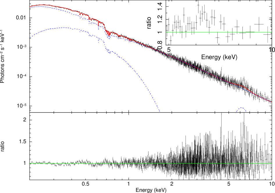
Figure 1.— XMM-Newton pn spectrum of Was 61 with fitted model (red) and data to model ratio. The model is a power-law (blue dot) plus a broad Gaussian component (blue dot) and a blackbody component (blue dot), which includes the Galactic absorption and a warm absorption. The top right is a zoomed plot in 5-10 keV for the data to model ratio with a power-law model.

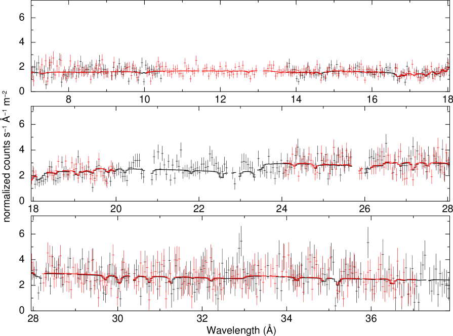
Figure 2.— The XMM-Newton RGS 1 (black) and RGS 2 (red) spectrum. Left panel: the same model as used in Figure 1; Right panel: the same model as used in the left one, but with its C, N, O, and Fe abundances of the absorber allowed to vary freely.

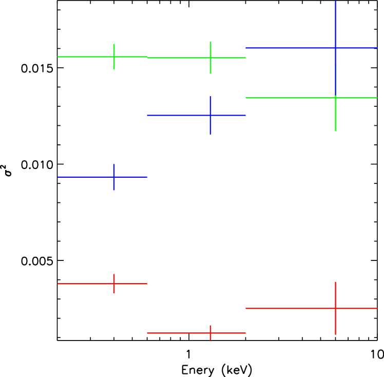
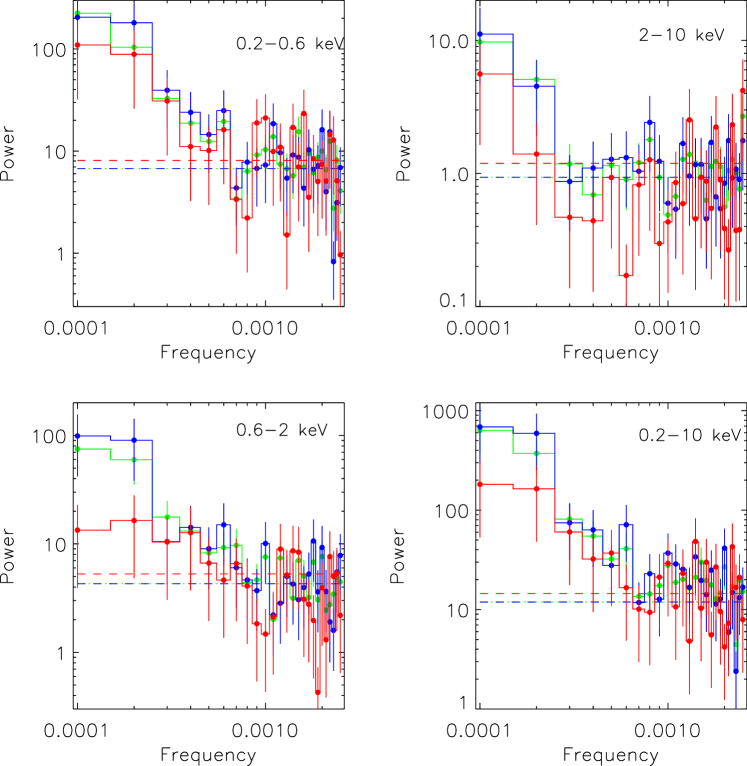
Figure 3.— Left panel: XMM-Newton lightcurves for Was 61 in each band. The time bin size is 200 s. The left is Obs1, the right is Obs2. The division of the four segments flagged as $L1$, $H1$, $H2$, and $L2$ state is illustrated in the 0.2-10 keV light curve. Middle panel: normalized excess variance of the Obs1 observation as a function of energy (the light curves is rebinned to 1 ks before calculating the NXS). Right panel: power spectral densities of Obs1 in each energy band, the lightcurve is rebinned to 200 s before creating the power spectral densities, the dashed line is the Poisson noise level (which is given as Vaughan et al. 2003). Green symbols are from the full exposure of Obs1, blue symbols are from the first 40 ks segment ($L1$+$H1$); and red symbols are from the last 20 ks segment ($H2$).

Figure 4.— Left panel: the Obs1 spectrum of Was 61, the Galactic absorbed power-law model inferred from fitting in 2-10 keV band and its extrapolation to the soft X-ray band is also shown; Right panel: the ratio of data to model in each state flagged as $L1$, $H1$, $H2$, and $L2$, comparing with the Obs1 spectrum.

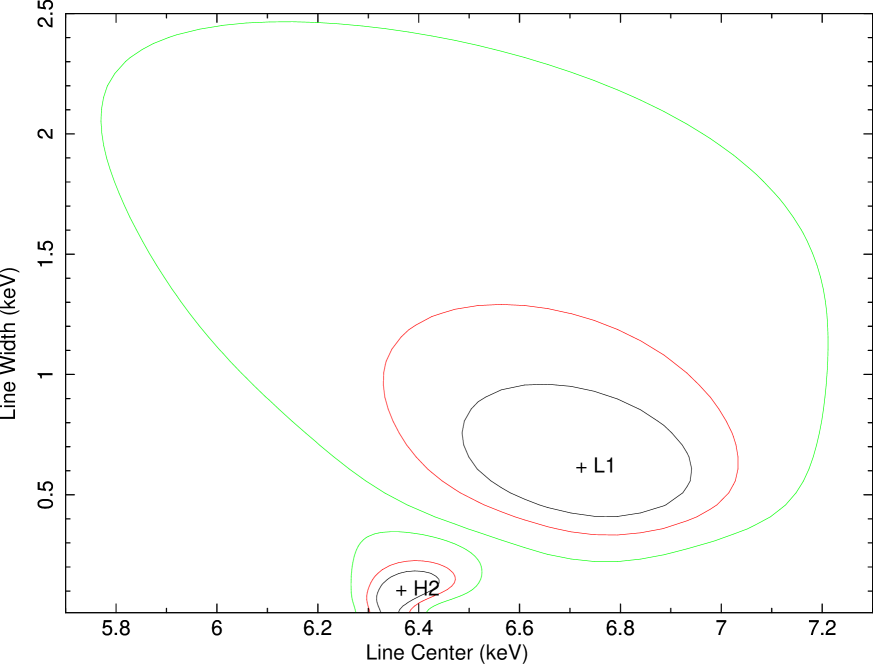
Figure 5.— Left panel: the spectrum in 2-10 keV and the ratio of data to model in each state. The photon index of the Galactic absorbed power-law model is fixed at 2.2 and the fitted Gaussian line model are also shown. Right Panel: confidence contours (at the 68%, 90%, and 99% confidence levels) of the line center and width of the Fe K line in $L1$ and $H2$.

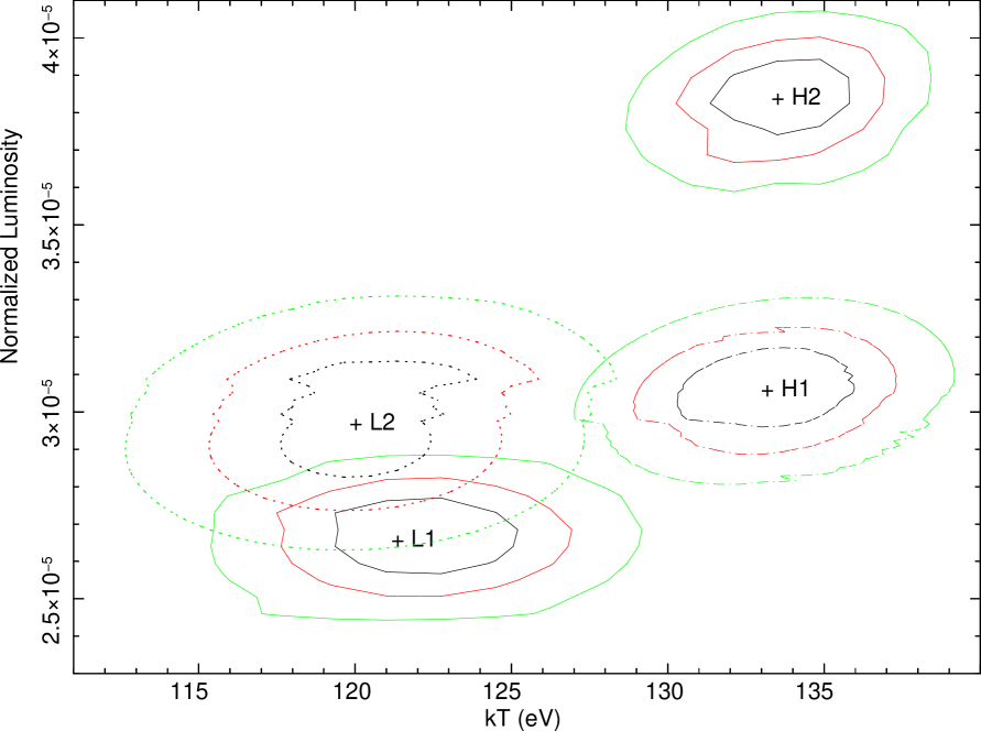
Figure 6.— Left panel: spectrum and the ratio of data to model in each state; the model is a power-law plus a broad Gaussian component and a blackbody component, which includes the Galactic absorption and a warm absorption. Right panel: confidence contours (at the 68%, 90%, and 99% confidence levels) of the normalization and temperature of the blackbody model

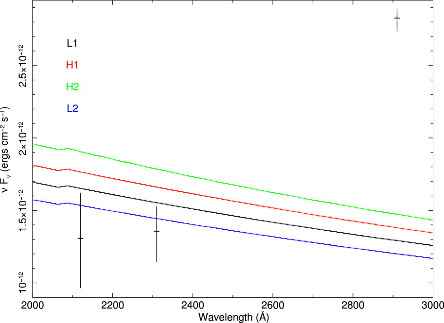
Figure 7.— Left panel: spectrum and the ratio of data to the model tbnew*warmabs*(optagnf+zgauss) in each state; Right panel: extrapolation the model of each state to 2000-3000Å, the symbols of the dots are the average fluxes of the OM observations with filters $UVW1$, $UVM2$, and $UVW2$ (with statistical errors 3%, 15% and 25%), respectively.

Table 1 Results of Fits to 2-10 keV Spectra

Model: tbnew*(Powerlaw)
	Powerlaw
	$\Gamma$	$L^{43}_{2-10}$	$\chi^{2}/dof$
	(1)	(2)	(6)
$obs1_{pn}$	$2.13\pm 0.03$	$1.95\pm 0.03$	497.9/520
$L1$	$2.04\pm 0.07$	$1.67\pm 0.13$	165.1/160
$H1$	$2.12\pm 0.05$	$2.00\pm 0.13$	207.4/232
$H2$	$2.17\pm 0.05$	$2.05\pm 0.03$	302.1/278
$L2$	$1.84\pm 0.07$	$1.84\pm 0.18$	90.8/102
Model: tbnew*(Powerlaw + zgauss)
	Powerlaw		Gauss
	$\Gamma$	$L^{43}_{2-10}$	$E_{center}$	$\sigma$	EW	$\chi^{2}/dof$
	(1)	(2)	(3)	(4)	(5)	(6)
$obs1_{pn}$	$2.17\pm 0.03$	$1.91\pm 0.03$	$6.43_{-0.28}^{+0.25}$	$0.49_{-0.26}^{+0.32}$	$0.22_{-0.03}^{+0.02}$	480.0/517
$L1$	$2.14\pm 0.08$	$1.60\pm 0.15$	$6.71_{-0.22}^{+0.28}$	$0.52_{-0.26}^{+0.32}$	$0.54^{+0.35}_{-0.26}$	146.7/157
$H1$	$2.15\pm 0.06$	$1.98\pm 0.14$	6.71(f)	0.52(f)	$0.11^{+0.14}_{-0.11}$	206.0/231
$H2$	$2.21\pm 0.05$	$2.02\pm 0.03$	$6.37_{-0.05}^{+0.06}$	$0.11_{-0.07}^{+0.06}$	$0.19^{+0.06}_{-0.06}$	278.7/276
$L2$	$1.88\pm 0.10$	$1.81\pm 0.22$	6.71(f)	0.52(f)	$0.13^{+0.22}_{-0.13}$	89.7/101
$L2$	$1.87\pm 0.08$	$1.81\pm 0.22$	6.37(f)	0.11(f)	$0.11^{+0.09}_{-0.09}$	87.0/101
$L1$	2.2(f)	$1.56\pm 0.04$	$6.73_{-0.27}^{+0.24}$	$0.62_{-0.22}^{+0.40}$	$0.74^{+0.28}_{-0.24}$	148.0/158
$H1$	2.2(f)	$1.94\pm 0.04$	6.73(f)	0.62(f)	$0.22^{+0.14}_{-0.15}$	208.4/232
$H2$	2.2(f)	$2.02\pm 0.03$	$6.37_{-0.06}^{+0.08}$	$0.11_{-0.08}^{+0.07}$	$0.19^{+0.06}_{-0.06}$	278.7/277
$L2$	2.2(f)	$1.52\pm 0.07$	6.73(f)	$2.08_{-0.56}^{+1.12}$	$2.71^{+1.18}_{-0.80}$	91.2/102
	Model: $\it{tbnew*(Powlaw+Diskline)}$, $\Gamma=2.2$
	$\it{Diskline}$
	$E_{center}$	$R_{in}$	$\chi^{2}/dof$
	(7)	(8)	(6)
L1	$6.81^{+0.58}_{-0.18}$	$6.2^{+24.8}_{-*}$	152.5/158
H2	$6.40^{+0.10}_{-0.07}$	$371.7_{-233.2}^{+428.2}$	279.2/276
Model: tbnew*pexrav
	pexrav
	$\Gamma$	$E_{cutoff}$	$rel_{refl}$	$\chi^{2}/dof$
	(9)	(10)	(11)	(6)
$L1$	$2.49_{-0.26}^{+0.35}$	100(f)	$5.5_{-3.3}^{+6.9}$	153.7/159
$L1$	2.2(f)	100(f)	$2.0_{-0.6}^{+0.6}$	157.2/160
$L2$	$1.88_{-0.13}^{+0.37}$	100(f)	$0.6_{-*}^{+3.9}$	90.6/101
$L2$	2.2(f)	100(f)	$3.9_{-0.9}^{+1.0}$	92.7/102
Model: tbnew*pexriv
	pexriv
	$\Gamma$	$E_{cutoff}$	$rel_{refl}$	$\xi$	$\chi^{2}/dof$
	(9)	(10)	(11)	(12)	(6)
$L1$	$2.49_{-0.23}^{+0.31}$	100(f)	$4.2_{-2.3}^{+5.1}$	$218.6_{-218.1}^{+1528.9}$	148.9/158
$L1$	2.2(f)	100(f)	$1.5_{-0.5}^{+0.7}$	$149.5_{-149.4}^{+1104.0}$	153.3/159
$L2$	$1.98_{-0.17}^{+0.22}$	100(f)	$0.9_{-0.5}^{+1.5}$	$4999.2_{-4830.1}^{+*}$	86.13/100
$L2$	2.2(f)	100(f)	$2.3_{-0.6}^{+0.5}$	$4999.8_{-4889.9}^{+*}$	88.7/101

• The columns are (1)-(2), the photon index $\Gamma$, the 2-10 keV luminosity in rest frame (in unit 10⁴³ erg s^-1) with the absorbing column removed of the power-law component; (3)-(5) the energy line center (in unit keV), the one $\sigma$ line width (in unit keV), and the equivalent width (in unit keV) of the Gaussian line component; (6) the $\chi^{2}$ and degree of freedom; (7)-(8) the energy line center in the rest frame (in unit keV) and the inner radius (in unit GM/c²) of the diskline model; (9)-(11) the first power-law photon index, the cutoff energy (keV) and the reflection scaling factor of the pexrav or pexriv model; (12) the disk ionization parameter of the pexriv model (in unit erg cm s^-1). The uncertainties are given at 90% confidence levels for one interesting parameter.

Table 2 Results of Broadband Spectral Fits for blackbody Models

Model: $\it{tbnew*warmabs*(powerlaw+zbbody+zgauss)}$
	Powerlaw			Blackbody		zgauss			warmabs
	$\Gamma$	$L^{43}_{0.2-2}$	$L^{43}_{2-10}$	$\it{kT}$	$L^{43}_{0.2-2}$	Ecenter	$\sigma$	EW	$N_{H}^{21}$	$\xi$	$\chi^{2}/dof$
	(1)	(2)	(3)	(4)	(5)	(6)	(7)	(8)	(9)	(10)	(11)
$obs1_{pn}$	$2.21\pm 0.02$	$4.13\pm 0.05$	$1.91\pm 0.02$	$135.1_{-4.3}^{+2.0}$	$1.19_{-0.20}^{+0.07}$	$6.41_{-0.22}^{+0.27}$	$0.63_{-0.21}^{+0.22}$	$0.25_{-0.04}^{+0.07}$	$3.31_{-0.24}^{+0.12}$	$6.8_{-1.9}^{+0.66}$	927.4/875
$obs1_{RGS}$	2.2(f)	$\cdots$	$\cdots$	135(f)	$\cdots$	$\cdots$	$\cdots$	$\cdots$	$4.48_{-0.22}^{+0.40}$	$9.40_{-1.99}^{+1.11}$	1142.7/945
${\it ROSAT}$	2.2(f)	$1.57\pm 0.04$	$\cdots$	$102.2_{-4.6}^{+3.1}$	$1.24\pm 0.04$	$\cdots$	$\cdots$	$\cdots$	$2.72_{-0.68}^{+0.85}$	$<2$	152.0/123
$L1$	2.2(f)	$3.49\pm 0.07$	$1.61\pm 0.03$	$121.6_{-3.4}^{+4.2}$	$0.80\pm 0.04$	$6.71_{-0.22}^{+0.20}$	$0.58_{-0.13}^{+0.27}$	$0.66\pm 0.20$
$H1$	2.2(f)	$4.22\pm 0.05$	$1.95\pm 0.03$	$133.3_{-2.9}^{+2.0}$	$0.95\pm 0.03$	6.71(t)	0.58(t)	$0.19\pm 0.14$
$H2$	2.2(f)	$4.53\pm 0.05$	$2.09\pm 0.03$	$134.2_{-3.1}^{+2.9}$	$1.19\pm 0.05$	$6.37_{-0.06}^{+0.06}$	$0.11_{-0.07}^{+0.06}$	$0.17\pm 0.06$	$3.20\pm 0.16$	$6.06^{+1.97}_{-0.80}$	2183.9/2142
$L2$	2.2(f)	$3.30\pm 0.07$	$1.52\pm 0.03$	$120.1_{-3.4}^{+4.2}$	$0.89\pm 0.04$	6.71(t)	$2.27_{-0.52}^{+0.57}$	$2.86_{-0.71}^{+0.99}$

• The columns are (1)-(3) the photon index $\Gamma$, the 0.2-2 and 2-10 keV luminosity in rest frame (in unit 10⁴³ erg s^-1) with the absorbing column removed of the power-law component; (4)-(5) the temperture (in unit eV) and the 0.2-2 keV luminosity in rest frame (in unit 10⁴³ erg s^-1) with the absorbing column removed of the blackbody component; (6)-(8) the energy line center (in unit keV), the one $\sigma$ line width (in unit keV), and the equivalent width (in unit keV) of the Gaussian line component; (9)-(10) the Hydrogen column density (in unit 10²¹ cm^-2) and the ionization parameter $\xi$ ($\xi$=L/nR², in unit erg cm s^-1, see Done et al. 1992) of the warm absorber; (11) the $\chi^{2}$ and degree of freedom.

Table 3Results of Broadband Spectral Fits for reflection Models

Model: $tbnew*warmabs*(powerlaw+kdblur*reflionx+zgauss)$

Powerlaw

kdblur*reflionx

zgauss

warmabs

$\Gamma$

norm1

$R_{in}$

Incl

$\xi_{r}$

norm2

Ecenter

$\sigma$

norm3

$N_{H}^{21}$

$\xi$

$\chi^{2}$

10-3

$10^{-6}$

10-6

$10^{21}$

(1)

(2)

(3)

(4)

(5)

(6)

(7)

(8)

(9)

(10)

(11)

(12)

$obs1_{pn}$

$2.33\pm 0.01$

$2.46\pm 0.02$

$4.41^{+0.28}_{-0.56}$

$0.1^{+0.1}_{-0.1}$

$11.9^{+0.9}_{-0.7}$

$4.5^{+0.3}_{-0.2}$

$6.68_{-0.19}^{+0.20}$

$0.34_{-0.14}^{+0.23}$

$6.6^{+3.4}_{-2.7}$

$2.8\pm 0.1$

$11.3^{+2.3}_{-0.6}$

971.4/873

$L1$

$2.02\pm 0.02$

$4.6^{+0.3}_{-0.2}$

$6.84_{-0.23}^{+0.18}$

$0.56_{-0.21}^{+0.19}$

$19.3^{+0.7}_{-0.5}$

$H1$

$2.33\pm 0.01$

$2.48\pm 0.02$

$3.28^{+0.47}_{-0.31}$

$21.1^{+3.3}_{-5.0}$

$10.4^{+0.4}_{-*}$

$5.1^{+0.2}_{-0.3}$

6.84(t)

0.56(t)

$7.2^{+6.9}_{-4.2}$

$2.8\pm 0.1$

$12.9^{+0.2}_{-2.2}$

2283.9/2139

$H2$

$2.69\pm 0.02$

$6.5^{+0.2}_{-0.3}$

$6.36_{-0.06}^{+0.04}$

$0.04_{-0.04}^{+0.11}$

$5.5^{+2.3}_{-2.5}$

$L2$

$1.91\pm 0.02$

$5.6^{+0.4}_{-0.3}$

6.84(t)

$2.28_{-0.51}^{+0.81}$

$78.0^{+18.7}_{-15.9}$

• The columns are: (1)-(2) the photon index $\Gamma$, the normazation in 10^-3 photons keV^-1 cm^-2 s^-1 at 1 keV of the power-law component; (3)-(6) the inner radius (in unit GM/c²), the inclination (in unit degree), the ionization parameter $\xi_{r}$ ($\xi_{r}$=F/nR², in unit erg cm s^-1), the normalization ($\times$10^-6) of the relativistic blurred reflected spectrum; (7)-(9) the energy line center (in unit keV), the one $\sigma$ line width (in unit keV), and total 10^-6 photons cm^-2 s^-1 of the Gaussian line component; (10)-(11) the Hydrogen column density (in unit $10^{21}$ cm^-2), and the ionization parameter $\xi$; (12) the $\chi^{2}$ and degree of freedom.

Table 4 Results of Broadband Spectral Fits for Comptonization Models

Model: $\it{tbnew*warmabs*(optxagnf+zgauss)}$, $\Gamma=2.2$, $M_{BH}=4.6\times 10^{6}$ M☉
	optxagnf
	$r_{cor}$	$\tau$	$\it{kT}$	$f_{pl}$	$L/L_{Edd}$	$\chi^{2}/dof$
	(1)	(2)	(3)	(4)	(5)	(6)
$obs1_{pn}$	$24.7_{-0.5}^{+0.5}$	$88.7^{+*}_{-31.6}$	$135.1_{-2.9}^{+6.1}$	$0.90_{-0.01}^{+0.01}$	$0.27\pm 0.01$	929.8/879
$L1$	$21.4_{-0.8}^{+0.8}$	$51.8^{+10.3}_{-6.4}$	$136.2_{-5.1}^{+4.8}$	$0.89_{-0.02}^{+0.02}$	$0.24\pm 0.02$
$H1$	$27.3_{-0.6}^{+1.1}$	$100^{+*}_{-23.7}$	$135.5_{-3.4}^{+3.3}$	$0.91_{-0.01}^{+0.01}$	$0.26\pm 0.02$
$H2$	$57.3_{-4.3}^{+4.1}$	$52.1^{+2.6}_{-2.3}$	$145.4_{-3.4}^{+2.8}$	$0.89_{-0.02}^{+0.02}$	$0.29\pm 0.01$	2162.9/2138
$L2$	$26.5_{-1.0}^{+1.8}$	$100^{+*}_{-47.6}$	$122.2_{-4.0}^{+5.3}$	$0.89_{-0.02}^{+0.01}$	$0.22\pm 0.02$
$L1$	$18.2_{-0.4}^{+0.5}$			$0.89_{-0.01}^{+0.01}$	$0.25\pm 0.01$
$H1$	$32.5_{-3.9}^{+14.1}$			$0.91_{-0.01}^{+0.01}$	$0.26\pm 0.01$
$H2$	$29.7_{-5.8}^{+4.7}$	$88.1^{+*}_{-22.4}$	$137.3_{-2.7}^{+3.9}$	$0.89_{-0.01}^{+0.01}$	$0.28\pm 0.01$	2184.1/2148
$L2$	$18.0_{-0.6}^{+0.7}$			$0.88_{-0.01}^{+0.01}$	$0.24\pm 0.01$
$L1$		$46.6^{+9.2}_{-5.3}$		$0.88_{-0.01}^{+0.01}$	$0.23\pm 0.01$
$H1$		$99.9^{+*}_{-32.7}$		$0.91_{-0.01}^{+0.01}$	$0.27\pm 0.01$
$H2$	$25.6_{-2.9}^{+4.8}$	$90.1^{+*}_{-25.5}$	$136.2_{-5.6}^{+3.8}$	$0.89_{-0.01}^{+0.01}$	$0.29\pm 0.01$	2171.0/2148
$L2$		$47.5^{+8.0}_{-5.7}$		$0.87_{-0.01}^{+0.02}$	$0.22\pm 0.01$
$L1$			$126.2_{-4.6}^{+6.8}$	$0.88_{-0.01}^{+0.01}$	$0.23\pm 0.01$
$H1$			$138.5_{-4.6}^{+6.1}$	$0.90_{-0.01}^{+0.01}$	$0.27\pm 0.01$
$H2$	$24.0_{-1.9}^{+5.7}$	$86.7^{+*}_{-33.0}$	$139.3_{-4.4}^{+6.3}$	$0.89_{-0.01}^{+0.01}$	$0.29\pm 0.01$	2171.8/2148
$L2$			$124.2_{-4.6}^{+6.3}$	$0.87_{-0.01}^{+0.02}$	$0.22\pm 0.01$
$L1$				$0.90_{-0.01}^{+0.01}$	$0.22\pm 0.01$
$H1$				$0.90_{-0.01}^{+0.01}$	$0.26\pm 0.01$
$H2$	$28.3_{-4.6}^{+*}$	$67.2^{+*}_{-18.0}$	$136.8_{-5.3}^{+6.0}$	$0.89_{-0.01}^{+0.01}$	$0.29\pm 0.01$	2206.1/2151
$L2$				$0.88_{-0.01}^{+0.02}$	$0.21\pm 0.01$
$L1$					$0.22\pm 0.01$
$H1$					$0.26\pm 0.01$
$H2$	$27.5_{-4.3}^{+*}$	$67.2^{+*}_{-18.3}$	$137.1_{-6.0}^{+5.5}$	$0.89_{-0.01}^{+0.01}$	$0.29\pm 0.01$	2229.3/2154
$L2$					$0.21\pm 0.01$

• The columns are: (1)-(5) the coronal radius r_cor (in unit R_g=GM/c²), the optical depth $\tau$ of the soft Comptonization component, the electron temperature $kT$ for the soft Comptonization component (soft excess) in eV, the fraction of the power below r_cor that is emitted in the hard Comptonization component, and the Eddington ratio of the optxagnf model; (6) the $\chi^{2}$ and degree of freedom.

References

- Abramowicz et al. (1988) Abramowicz, M. A.,Czerny, B., Lasota, J. P., & Szuszkiewicz, E. 1988, ApJ, 332, 646
- Ai et al. (2011) Ai, Y. L., Yuan, W., Zhou, H. Y., Wang, T. G., & Zhang, S. H. 2011, ApJ, 727, 31
- Arav et al. (2015) Arav, N., Chamberlain, C., Kriss, G. A., et al. 2015, A&A, 577, A37
- Arnaud (1996) Arnaud, K. A. 1996, Astronomical Data Analysis Software and Systems V, 101, 17
- Avni (1976) Avni, Y. 1976, ApJ, 209, 574
- Bian & Zhao (2003) Bian, W., & Zhao, Y. 2003, ApJ, 591, 733
- Bianchi et al. (2009) Bianchi, S., Guainazzi, M., Matt, G., Fonseca Bonilla, N., & Ponti, G. 2009, A&A, 495, 421
- Blustin et al. (2005) Blustin, A. J., Page, M. J., Fuerst, S. V., Branduardi-Raymont, G., & Ashton, C. E. 2005, A&A, 431, 111
- Brenneman et al. (2014a) Brenneman, L. W., Madejski, G., Fuerst, F., et al. 2014a, ApJ, 788, 61
- Brenneman et al. (2014b) Brenneman, L. W., Madejski, G., Fuerst, F., et al. 2014b, ApJ, 781, 83
- Brenneman et al. (2011) Brenneman, L. W., Reynolds, C. S., Nowak, M. A., et al. 2011, ApJ, 736, 103
- Cackett et al. (2013) Cackett, E. M., Fabian, A. C., Zogbhi, A., et al. 2013, ApJ, 764, L9
- Cackett et al. (2014) Cackett, E. M., Zoghbi, A., Reynolds, C., et al. 2014, MNRAS, 438, 2980
- Cheng et al. (2002) Cheng, L.-P., Wei, J.-Y., & Zhao, Y.-H. 2002, ChJA&A, 2, 207
- Crummy et al. (2006) Crummy, J., Fabian, A. C., Gallo, L., & Ross, R. R. 2006, MNRAS, 365, 1067
- Czerny & Elvis (1987) Czerny, B., & Elvis, M. 1987, ApJ, 321, 305
- Czerny et al. (2003) Czerny, B., Nikołajuk, M., Różańska, A., et al. 2003, A&A, 412, 317
- de Marco et al. (2011) de Marco, B., Ponti, G., Uttley, P., et al. 2011, MNRAS, 417, L98
- de La Calle Pérez et al. (2010) de La Calle Pérez, I., Longinotti, A. L., Guainazzi, M., et al. 2010, A&A, 524, A50
- Done et al. (2012) Done, C., Davis, S. W., Jin, C., Blaes, O., & Ward, M. 2012, MNRAS, 420, 1848
- Done et al. (1992) Done, C., Mulchaey, J. S., Mushotzky, R. F., & Arnaud, K. A. 1992, ApJ, 395, 275
- Du et al. (2014) Du, P., Hu, C., Lu, K.-X., et al. 2014, ApJ, 782, 45
- Emmanoulopoulos et al. (2011) Emmanoulopoulos, D., McHardy, I. M., & Papadakis, I. E. 2011, MNRAS, 416, L94
- Fabian (2006) Fabian, A. C. 2006, Astronomische Nachrichten, 327, 943
- Fabian (2008) Fabian, A. C. 2008, Astronomische Nachrichten, 329, 155
- Fabian et al. (2000) Fabian, A. C., Iwasawa, K., Reynolds, C. S., & Young, A. J. 2000, PASP, 112, 1145
- Fabian et al. (2004) Fabian, A. C., Miniutti, G., Gallo, L., et al. 2004,MNRAS, 353, 1071
- Fabian et al. (1989) Fabian, A. C., Rees, M. J., Stella, L., & White, N. E. 1989, MNRAS, 238, 729
- Fabian et al. (2009) Fabian, A. C., Zoghbi, A., Ross, R. R., et al. 2009, Nature, 459, 540
- Fabian et al. (2012) Fabian, A. C., Zoghbi, A., Wilkins, D., et al. 2012, MNRAS, 419, 116
- Gallo et al. (2015) Gallo, L. C., Wilkins, D.R., Bonson, K. et al. 2015, MNRAS, 446, 633
- Gardner & Done (2014) Gardner, E., & Done, C. 2014, MNRAS, 442, 2456
- George et al. (1998) George, I. M., Turner, T. J., Netzer, H., et al. 1998, ApJS, 114, 73
- Gierliński & Done (2004) Gierliński, M., & Done, C. 2004, MNRAS, 349, L7
- Grupe et al. (1999a) Grupe, D., Beuermann, K., Mannheim, K., & Thomas, H.-C. 1999a, A&A, 350, 805
- Grupe et al. (2001) Grupe, D., Thomas, H.-C., & Beuermann, K. 2001, A&A, 367, 470
- Grupe et al. (2004) Grupe, D., Wills, B. J., Leighly, K. M., & Meusinger, H. 2004, AJ, 127, 156
- Grupe et al. (1999b) Grupe, D., Wills, B. J., & Wills, D. 1999b, Structure and Kinematics of Quasar Broad Line Regions, 175, 347
- Guainazzi et al. (2006) Guainazzi, M., Bianchi, S., & Dovčiak, M. 2006, Astronomische Nachrichten, 327, 1032
- Haardt & Maraschi (1991) Haardt, F., & Maraschi, L. 1991, ApJ, 380, L51
- Halpern (1984) Halpern, J. P. 1984, ApJ, 281, 90
- Jovanović (2012) Jovanović, P. 2012, NewAR, 56, 37
- Kalberla et al. (2005) Kalberla, P. M. W., Burton, W. B., Hartmann, D., et al. 2005, A&A, 440, 775
- Kallman & Bautista (2001) Kallman, T., & Bautista, M. 2001, ApJS, 133, 221
- Kara et al. (2014) Kara, E., Cackett, E. M., Fabian, A. C., Reynolds, C., & Uttley, P. 2014, MNRAS, 439, L26
- Kara et al. (2013a) Kara, E., Fabian, A. C., Cackett, E. M., et al. 2013, MNRAS, 428, 2795
- Kara et al. (2013b) Kara, E., Fabian, A. C., Cackett, E. M., et al. 2013, MNRAS, 434, 1129
- Kaspi et al. (2002) Kaspi, S., Brandt, W. N., George, I. M., et al. 2002, ApJ, 574, 643
- Kaspi et al. (2000) Kaspi, S., Brandt, W. N., Netzer, H., et al. 2000, ApJ, 535, L17
- Keel et al. (1988) Keel, W. C., de Grijp, M. H. K., & Miley, G. K. 1988, A&A, 203, 250
- Krolik & Kriss (2001) Krolik, J. H., & Kriss, G. A. 2001, ApJ, 561, 684
- Krongold et al. (2007) Krongold, Y., Nicastro, F., Elvis, M., et al. 2007, ApJ, 659, 1022
- Laha et al. (2013) Laha, S., Dewangan, G. C., Chakravorty, S., & Kembhavi, A. K. 2013, ApJ, 777, 2
- Laor (1991) Laor, A. 1991, ApJ, 376, 90
- Lee et al. (2001) Lee, J. C., Ogle, P. M., Canizares, C. R., et al. 2001, ApJ, 554, L13
- Lee et al. (2009) Lee, J. C., Xiang, J., Ravel, B., Kortright, J., & Flanagan, K. 2009, ApJ, 702, 970
- Liu et al. (2014) Liu, T., Wang, J.-X., Yang, H., Zhu, F.-F., & Zhou, Y.-Y. 2014, ApJ, 783, 106
- Liu et al. (2015) Liu, Z., Yuan, W., Lu, Y., & Zhou, X. 2015, MNRAS, 447, 517
- Lohfink et al. (2012) Lohfink, A. M., Reynolds, C. S., Miller, J. M., et al. 2012, ApJ, 758, 67
- Longinotti et al. (2004) Longinotti, A. L., Nandra, K., Petrucci, P. O., & O’Neill, P. M. 2004, MNRAS, 355, 929
- Marinucci et al. (2014) Marinucci, A., Matt, G., Kara, E., et al. 2014, MNRAS, 440, 2347
- Markowitz et al. (2003) Markowitz, A., Edelson, R., & Vaughan, S. 2003, ApJ, 598, 935
- McHardy et al. (2006) McHardy, I. M.,Koerding, E., Knigge, C., Uttley, P., & Fender, R. P. 2006, Nature, 444, 730
- Mushotzky et al. (1993) Mushotzky, R. F., Done, C., & Pounds, K. A. 1993, ARA&A, 31, 717
- Nandra et al. (2007) Nandra, K., O’Neill, P. M., George, I. M., & Reeves, J. N. 2007, MNRAS, 382, 194
- Nardini et al. (2011) Nardini, E., Fabian, A. C., Reis, R. C., & Walton, D. J. 2011, MNRAS, 410, 1251
- Nowak et al. (2012) Nowak, M. A., Neilsen, J., Markoff, S. B., et al. 2012, ApJ, 759, 95
- Pal & Dewangan (2013) Pal, M., & Dewangan, G. C. 2013, MNRAS, 435, 1287
- Patrick et al. (2012) Patrick, A. R., Reeves, J. N., Porquet, D., et al. 2012, MNRAS, 426, 2522
- Petrucci et al. (2002) Petrucci, P. O., Henri, G., Maraschi, L., et al. 2002, A&A, 388, L5
- Pollack (2015) Pollack, A.M.T. 2015, “Status of the RGS Calibration”, XMM-SOC-CAL-TN-0030 issue 7.4
- Ponti et al. (2012) Ponti, G., Papadakis, I., Bianchi, S., et al. 2012, A&A, 542, A83
- Porquet et al. (2004) Porquet, D., Reeves, J. N., O’Brien, P., & Brinkmann, W. 2004, A&A, 422, 85
- Pounds et al. (1990) Pounds, K. A., Nandra, K., Stewart, G. C., George, I. M., & Fabian, A. C. 1990, Nature, 344, 132
- Predehl & Schmitt (1995) Predehl, P., & Schmitt, J. H. M. M. 1995, A&A, 293, 889
- Reynolds (1997) Reynolds, C. S. 1997, MNRAS, 286, 513
- Risaliti et al. (2013) Risaliti, G., Harrison, F. A., Madsen, K. K., et al. 2013, Nature, 494, 449
- Ross & Fabian (1993) Ross, R. R., & Fabian, A. C. 1993, MNRAS, 261, 74
- Ross & Fabian (2005) Ross, R. R., & Fabian, A. C. 2005, MNRAS, 358, 211
- Sako et al. (2003) Sako, M., Kahn, S. M., Branduardi-Raymont, G., et al. 2003, ApJ, 596, 114
- Shimura & Takahara (1993) Shimura, T., & Takahara, F. 1993, ApJ, 419, 78
- Shu et al. (2012) Shu, X. W., Wang, J. X., Yaqoob, T., Jiang, P., & Zhou, Y. Y. 2012, ApJ, 744, L21
- Shu et al. (2010) Shu, X. W., Yaqoob, T., & Wang, J. X. 2010, ApJS, 187, 581
- Strüder et al. (2001) Strüder, L., Briel, U., Dennerl, K., et al. 2001, A&A, 365, L18
- Sun et al. (2013) Sun, L., Shu, X., & Wang, T. 2013, ApJ, 768, 167
- Tanaka et al. (1995) Tanaka, Y., Nandra, K., Fabian, A. C., et al. 1995, Nature, 375, 659
- Terashima et al. (2012) Terashima, Y., Kamizasa, N., Awaki, H., Kubota, A., & Ueda, Y. 2012, ApJ, 752, 154
- Treves et al. (1988) Treves, A., Maraschi, L., & Abramowicz, M. 1988, PASP, 100, 427
- Turner & Miller (2009) Turner, T. J., & Miller, L. 2009, A&A Rev., 17, 47
- Turner et al. (2007) Turner, T. J., Miller, L., Reeves, J. N., & Kraemer, S. B. 2007, A&A, 475, 121
- Turner et al. (2008) Turner, T. J., Reeves, J. N., Kraemer, S. B., & Miller, L. 2008, A&A, 483, 161
- Vasudevan et al. (2014) Vasudevan, R. V., Mushotzky, R. F., Reynolds, C. S., et al. 2014, ApJ, 785, 30
- Vaughan et al. (2003) Vaughan, S., Edelson, R., Warwick, R. S., & Uttley, P. 2003, MNRAS, 345, 1271
- Walton et al. (2013) Walton, D. J., Nardini, E., Fabian, A. C., Gallo, L. C., & Reis, R. C. 2013, MNRAS, 428, 2901
- Wandel & Petrosian (1988) Wandel, A., & Petrosian, V. 1988, ApJ, 329, L11
- Wilkins & Fabian (2012) Wilkins, D. R., & Fabian, A. C. 2012, MNRAS, 424, 1284
- Wilms et al. (2000) Wilms, J., Allen, A., & McCray, R. 2000, ApJ, 542, 914
- Xiao et al. (2012) Xiao, T., Wang, T., Wang, H., et al. 2012, MNRAS, 421, 486
- Yaqoob & Padmanabhan (2004) Yaqoob, T., & Padmanabhan, U. 2004, ApJ, 604, 63
- Yuan et al. (2010) Yuan, W., Liu, B. F., Zhou, H., & Wang, T. G. 2010, ApJ, 723, 508
- Zdziarski et al. (1994) Zdziarski, A. A., Fabian, A. C., Nandra, K., et al. 1994, MNRAS, 269, L55
- Zhong & Wang (2013) Zhong, X., & Wang, J. 2013, ApJ, 773, 23
- Zhou & Zhang (2010) Zhou, X.-L., & Zhang, S.-N. 2010, ApJ, 713, L11
- Zoghbi et al. (2014) Zoghbi, A., Cackett, E. M., Reynolds, C., et al. 2014, ApJ, 789, 56
- Zoghbi & Fabian (2011) Zoghbi, A., & Fabian, A. C. 2011, MNRAS, 418, 2642
- Zoghbi et al. (2012) Zoghbi, A., Fabian, A. C., Reynolds, C. S., & Cackett, E. M. 2012, MNRAS, 422, 129
- Zoghbi et al. (2010) Zoghbi, A., Fabian, A. C., Uttley, P., et al. 2010, MNRAS, 401, 2419
- Zoghbi et al. (2013) Zoghbi, A., Reynolds, C., Cackett, E. M., et al. 2013, ApJ, 767, 121