Large size and slow rotation of the trans-Neptunian object (225088) 2007 OR₁₀ discovered from Herschel and K2 observations

Abstract

We present the first comprehensive thermal and rotational analysis of the second most distant trans-Neptunian object (225088) 2007 OR₁₀. We combined optical light curves provided by the Kepler space telescope – K2 extended mission and thermal infrared data provided by the Herschel Space Observatory. We found that (225088) 2007 OR₁₀ is likely to be larger and darker than derived by earlier studies: we obtained a diameter of $d=1535^{+75}_{-225}\,{\rm km}$ which places (225088) 2007 OR₁₀ in the biggest top three trans-Neptunian objects. The corresponding visual geometric albedo is $p_{V}=0.089^{+0.031}_{-0.009}$. The light curve analysis revealed a slow rotation rate of $P_{\rm rot}=44.81\pm 0.37\,{\rm h}$, superseded by a very few objects only. The most likely light-curve solution is double-peaked with a slight asymmetry, however, we cannot safely rule out the possibility of having a rotation period of $P_{\rm rot}=22.40\pm 0.18\,{\rm h}$ which corresponds to a single-peaked solution. Due to the size and slow rotation, the shape of the object should be a MacLaurin ellipsoid, so the light variation should be caused by surface inhomogeneities. Its newly derived larger diameter also implies larger surface gravity and a more likely retention of volatiles – ${\rm CH}_{4}$, ${\rm CO}$ and ${\rm N}_{2}$ – on the surface.

1. Introduction

Trans-Neptunian objects (TNOs) are known as the most pristine types of bodies orbiting in the Solar System. Extending our knowledge of these objects helps us to understand both the formation of our planetary system and the interpretation of observational data regarding to circumstellar material or debris disks of other stars. (225088) 2007 OR₁₀, discovered by Schwamb et al. (2009), is the second most distant known TNO to date, following Eris: the current heliocentric distance of this object exceeds $87\,{\rm AU}$ and still moving further away up to its aphelion in year 2130 at $\sim 100.7\,{\rm AU}$. Its orbital eccentricity is high ($e\approx 0.51$), so upon perihelion, it comes nearly as close as Neptune. In addition, 2007 OR₁₀ is likely to be in the $3:10$ mean motion resonance with Neptune. Ground-based observations revealed a characteristic red color for this object: according to Boehnhardt et al. (2014), its $V-R$ color index is $0.86\pm 0.02$. Santos-Sanz et al. (2012) have studied 15 scattered disk objects (SDOs) and detached objects, including 2007 OR₁₀, where these objects have a series of far-infrared thermal measurements taken with the Herschel Space Observatory . The albedo of 2007 OR₁₀ was found to be $p_{R}\approx 18\%$ in $R$ band, hence this object is a member of the “bright & red” subgroup of the TNO population (Lacerda et al., 2014). The corresponding diameter of 2007 OR₁₀ was reported as $d=1280\pm 210\,{\rm km}$ (see also Table 5 in Santos-Sanz et al., 2012). The analysis of near-infrared spectra also revealed the presence of water ice absorption features (Brown, Burgasser & Fraser, 2011).

The Kepler space telescope has been designed to continuously observe a dedicated field close to the northern pole of the Ecliptic in order to discover and characterize transiting extrasolar planets (Borucki et al., 2010). After the failure of the reaction wheels, having only two available for fine attitude control, the new mission called K2 has been initiated and commissioned (Howell et al., 2014). In this extended mission, Kepler observes fields close to the ecliptic plane in a quarterly schedule. Due to the orientation of the solar panels on Kepler, these fields have a typical solar elongation between $\sim 140-50$ degrees during such a $\sim 3$ months long campaign.

Observing near the ecliptic has two relevant consequences. First, minor planets crossing the fields could seriously affect the photometric quality by intersecting the apertures of target stars (Szabó et al., 2015). Second, allocating dedicated pixel masks to these moving Solar System objects can provide a unique way to gather uninterrupted photometric time series. This can further be relevant for TNOs where the apparent mean motion is slow: as it has been demonstrated by Pál et al. (2015a), even small stamps having a size of $\sim 20\times 20$ pixels could include the arc of a TNO around its stationary point (which is also observed in a K2 campaign, see the typical solar elongation range above). To date, the K2 mission has been involved in the precise detection of rotation light variations of the objects (278361) 2007 JJ₄₃, 2002 GV₃₁ (Pál et al., 2015a) and Nereid, a satellite of Neptune (Kiss et al., 2016). In this work we extend this sample with (225088) 2007 OR₁₀.

Up to now, no rotational brightness variation has been detected for 2007 OR₁₀: the upper limit for a light curve amplitude found by Benecchi & Sheppard (2013) is $<0.09\,{\rm mag}$. Using K2 observations, we present the first detection of optical brightness variations of this object, detecting a slow, likely double-peaked rotation with a corresponding low amplitude light curve. This information is further used to characterize the physical properties of the surface of 2007 OR₁₀ by employing thermophysical models. In Sec. 2, we describe the observations and data reduction related to K2 and the re-reduction of Herschel/PACS scan map data. In Sec. 3, we briefly detail the methods used to analyze the optical light curve. The description of the accurate thermal modelling is found in Sec. 4. In Sec. 5, we summarize our results.

2. Observations and data reduction

2.1. Kepler/K2 observations and data reduction

Kepler observed the apparent track of 2007 OR₁₀ in K2 Campaign 3 under the Guest Observer Office proposal GO3053. The track has been covered by two custom aperture masks following the trajectory of the object with a width of $10-11$ pixels on average. Unfortunately, the apparent stationary point of the object, viewed from Kepler, was located in the gap between the two CCDs of module #18 (in fact, in the gap between channels 2 and 3).

Hence, the first pixel mask covered the first $\sim 15$ days of Campaign 3 while the second pixel mask covered only the last $\sim 5$ days of the planned interval. Another unfortunate constellation is the apparent vicinity of the bright star 45 Aquarii (HD 211676), which has a brightness of $V=5.9$. The systematics induced by the halo and the diffraction spikes of 45 Aquarii significantly decrease the attainable signal-to-noise ratio even in the case of a moving object. However, Campaign 3 ended prematurely after $69.2$ days, about $10$ days short of the planned length of the campaign, therefore 2007 OR₁₀ did not appear in the mask closer to 45 Aqr at all (Thompson, 2015). Overall, Kepler followed the light variations of 2007 OR₁₀ for 12.0 days continuously. The elongation of the object decreased from $140$ to $70$ degrees during the campaign but due to the aforementioned facts, only the elongations between $140$ and $123$ degrees were available for further analysis.

The data series for the track of 2007 OR₁₀ as well as the comparison stars has a timing cadence corresponding to K2 long-cadence mode, i.e. $0.0204\,{\rm d}$ (approximately $29.4$ minutes). These long-cadence stamps are summed from $270$ individual exposures onboard (in order to save telemetric bandwidth). Each exposure has a net (useful) integration time of $6.02\,{\rm sec}$, while $\sim 8\%$ of the time is spent by readout (see also Gilliland et al., 2010, for more details).

The public target pixel time series files from the Campaign 3 fields were retrieved from the MAST archive for the respective observations. In addition to the two masks corresponding to the parts of the sky covering the apparent arc of 2007 OR₁₀, we retrieved a dozen of masks related to nearby additional sources. The analyzed field-of-view of module #18 channel 2 has been displayed in Fig. 1. Since the masks corresponding to the apparent trajectory of 2007 OR₁₀ do not contain bright background stars, we used the information provided by 10 of the unsaturated point sources presented on these additional masks to obtain a relative (differential) and absolute astrometric solutions needed by the photometric pipeline. In this sense, this type of astrometric bootstrapping was simpler than the case of 2007 JJ₄₃ where only the stars located in the mask corresponding to the object’s path were used (see Pál et al., 2015a, for further details).

The analysis of the frames has been performed in a highly similar manner as it was done in the previous K2 observations (Pál et al., 2015a). The most relevant improvement in our pipeline is the inclusion of the aforementioned 10 additional stamps which provide a more accurate astrometric reference system w.r.t. the Kepler CCDs. For all of the processing steps, including the extraction of K2 data files, we involved the tasks of the FITSH package (Pál, 2012). As in our previous work (Pál et al., 2015a), instrumental magnitudes were derived using differential photometry which is a relatively easy task for moving objects when the instrumental point-spread function is stable. Individual differential points had a formal uncertainty of $0.07-0.10$ mags on average, corresponding to a signal-to-noise ratio of $10-14$. This is in the range of our expectations considering both moving objects (Pál et al., 2015a) and faint stationary objects in the brightness regime of $\sim 21$ mags in the original and K2 missions (Molnár et al., 2015; Olling et al., 2015).

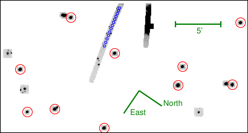
Figure 1.— The total analyzed field-of-view of the Kepler, showing both the stamps related to (225088) 2007 OR₁₀ as well as the nearby image stamps used for astrometry. The stars used by the determination for both the differential and absolute astrometric solutions are indicated by red circles. The field has a pixel dimension of $410\times 220$, equivalent to $27^{\prime}\times 15^{\prime}$. Note that the pixels are shown in the reference frame of the detector and therefore the image itself is flipped. Note also that the edge of channel 2 of module #18 is at the top of the image.

Table 1Photometric data of 2007 OR₁₀.

Time (JD)	Magnitudea	Error
2456982.00186	20.942	0.087
2456982.02229	20.951	0.080
2456982.04272	20.900	0.075

Note. — Table 1 is published in its entirety in the electronic edition of the Astronomical Journal. A portion is shown here for guidance regarding its form and content.

The photometric magnitudes of 2007 OR₁₀ have been transformed into USNO-B1.0 $R$ system (Monet et al., 2003). In order to find the transformation coefficients, we fitted 10 of the additional stars included in the analysis (originally selected for astrometric purposes). We found that the unbiased residual of the photometric transformation between USNO-B1.0 and Kepler unfiltered magnitudes was $0.09\,{\rm mag}$. The magnitude of these stars used for this transformation were in the range of $R=11$ and $R=14$ (i.e. somewhat brighter regime what was used in the case of (278361) 2007 JJ₄₃ earlier).

We note here that the intrinsic red color of 2007 OR₁₀ and the unfiltered nature of Kepler observations make this type of transformation and hence the yielded magnitudes not be suitable for physical interpretation. Indeed, the absolute magnitude of 2007 OR₁₀ in $R$ band (see Sec. 4 later on) combined with the observation geometry at the time of the usable K2 observations yields an expected $R$ magnitude of $20.88$ while the median of the light curve is $21.17$ magnitudes. This difference of $\sim 0.3$ magnitudes is significantly larger than the residual of the photometric transformation and even large to be accounted for phase effects. The photometric time series data of 2007 OR₁₀ are shown in Table 1 (the full table is available in an electronic form). In order to reject the outlier points, we performed an iterative sigma-clipping procedure in the binned light curves. This procedure has significantly decreased the light curve RMS, showing that these outlier points were caused by non-Gaussian random effects (systematics on the detector, cosmic hits, etc).

The photometric quality can easily be quantified as follows. If one has a time series of magnitudes and their respective uncertainties (as derived by the photometric pipeline run on each image separately), then one can compare the model fit residuals w.r.t these uncertainties. In our case, we consider the folded and binned light curve as a “model fit” If the ratio of these two numbers are close to unity, it means that the photometric quality (i.e. the overall efficiency of the photometric pipeline) is nearly perfect – independently of the actual values of the uncertainties. In our case, these values are $\sim 0.11$ (the mean of RMS around the binned points) and $\sim 0.08$ (the mean value of the photometric uncertainties as reported by FITSH/fiphot). It means that the photometric quality can be considered adequate but indeed there could be options to further tune in the algorithms. It can even mean the more sophisticated rejection of outliers (due to cosmic hits or prominent residual structures on the differential images, etc) could further push this ratio down to or at least, closer to unity. We note here that this ratio of $0.11/0.08\approx 1.4$ is even better what was found in the case of (278361) 2007 JJ₄₃, where it is $\sim 1.7$ or what was found for Nereid ($\sim 1.8$) but worse than what can be derived for 2002 GV₃₁ for which it is $\sim 1.1$. These comparison can also be done using the publicly available data for these three objects (Pál et al., 2015a; Kiss et al., 2016). We also note that the similar median stacking procedure which was involved during the analysis of 2002 GV₃₁ cannot be applied for these K2 observations of 2007 OR₁₀ since the apparent mean motion was much higher (i.e. 2002 GV₃₁ was observed during its stationary point while images for 2007 OR₁₀ are available only at the beginning of the campaign, far off the stationary point). By increasing the sample of photometric data series of moving objects acquired by K2, we could provide algorithms which would yield more precise light curves. According to the current sample of three such observations, the respective light curve of 2007 OR₁₀ has an “average quality” in this sense.

Table 2Orbital and optical data for 2007 OR₁₀.

Quantity	Symbol	Value
Heliocentric distance	$r$	$86.331$ AU
Distance from Herschel	$\Delta$	$86.586$ AU
Phase angle	$\alpha$	$0.\!\!^{\circ}65$
Absolute visual magnitude	$H_{V}$	$2.34\pm 0.05$
Absolute $R$ magnitude	$H_{R}$	$1.49\pm 0.05$

Note. — The above data are for the midpoint of Herschel observations, i.e. 2011 May 8. These parameters were incorporated throughout the thermal analysis.

2.2. Herschel/PACS observations and data reduction

In the framework of the “TNO’s are Cool!” Open Time Key Programme (Müller et al., 2009) of the Herschel Space Observatory (Pilbratt et al., 2010), the object 2007 OR₁₀ has been observed in a similar fashion like the another $130+$ trans-Neptunian targets of this project (Kiss et al., 2014). The aim was to employ the Photoconductor Array Camera and Spectrometer (PACS, Poglitsch et al., 2010) instrument of Herschel to provide thermal flux estimations for these objects in the wavelength range of $60-210\,{\rm\mu m}$. Since the expected temperature of a trans-Neptunian object is in the range of few tens of Kelvins, the PACS instrument provides an efficient way to characterize the thermal radiation of these bodies. Once the thermal fluxes are known, the combination with the optical absolute brightness and rotation period yields an unambiguous estimation of the size and albedo.

In brief, a TNO, like 2007 OR₁₀ has been observed twice in order to both estimate and reduce the effects of the background confusion noise. This is an essential step since the structure of the background is unknown due to the lack of any former or recent survey providing imaging data in this wavelength regime. The summary of Herschel/PACS observations is shown in Table 2 of Santos-Sanz et al. (2012). Earlier flux estimations have been performed and presented in Santos-Sanz et al. (2012) for 15 scattered disk and detached objects, including 2007 OR₁₀. However, we re-reduced the available Herschel/PACS data using the recent improvements in our HIPE-based (Ott, 2010) PACS data processing pipeline, presented in Kiss et al. (2014). This type of re-reduction involved not only the objects directly related to the “TNO’s are Cool!” programme, but exploited additional observations of recently discovered Solar System targets (see e.g. Pál et al., 2015b). The image stamps created by this so-called double-differential method (Kiss et al., 2014; Pál et al., 2015b) are displayed in Fig. 2.

Flux estimations have been performed using aperture photometry while the respective uncertainties have been derived using the artificial source implantation method (Kiss et al., 2014, see also). The derived uncertainties also include the additional $5\%$ due to the absolute flux level calibration error (Balog et al., 2014). The fluxes have been found to be $2.52\pm 1.20\,{\rm mJy}$, $5.68\pm 1.47\,{\rm mJy}$ and $6.71\pm 2.03\,{\rm mJy}$ in the “blue” ($60-85\,{\rm\mu m}$, centered at $70\,{\rm\mu m}$), “green” ($85-130\,{\rm\mu m}$, centered at $100\,{\rm\mu m}$) and “red” ($130-210\,{\rm\mu m}$, centered at $160\,{\rm\mu m}$) PACS bands. During the derivation of these fluxes, we also included the color correction factors of $C_{70}=0.992$, $C_{100}=0.985$ and $C_{160}=0.995$ corresponding to the temperature of $\sim 37\,{\rm K}$ for this object (see also Müller, Okumura & Klaas, 2011).

3. Optical light curve analysis

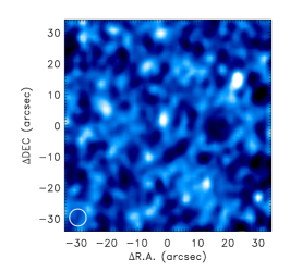
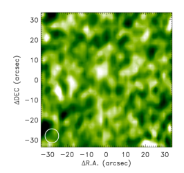
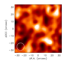
Figure 2.— Image stamps of (225088) 2007 OR₁₀ as seen by the PACS detector of Herschel. The stamps show the vicinity of the object and cover a $70^{\prime\prime}\times 70^{\prime\prime}$ area on the sky. From left to right, the stamps show the object in $70\,{\rm\mu m}$ (blue), $100\,{\rm\mu m}$ (green) and $160\,{\rm\mu m}$ (red) channels. The small white circles in the lower-left corner show the beam size (which is the largest in the red channel due to the diffraction-limited resolution of the instrument. Note that the object itself is slightly offset by $\approx 2^{\prime\prime}$ from the field center due to the pointing drifts and astrometric uncertainties with respect to the nominal coordinates.

Figure 3.— Left: phase-folded light curve of (225088) 2007 OR₁₀ superimposed with binned data points and the best-fit sinusoidal fit used for period search. The folding period corresponds to the suspected double-peak rotation period of $P_{\rm rot}=44.81\pm 0.37\,{\rm h}$. Right: Fourier transform of the photometric light variation of (225088) 2007 OR₁₀, as converted to false alarm probabilities, showing the prominent peak at $n=1.071\,{\rm cycles/day}$ and the respective false alarm probability of $1.7\times 10^{-7}$. This value corresponds to a detection of $5.2$-$\sigma$.

In order to find periodicity in the observed K2 photometric time series, we analyzed the light curve with the Period04 software (Lenz & Breger, 2005). The Fourier transform of the data revealed a single periodicity with a signal-to-noise ratio higher than 5.0, at $n=1.071\pm 0.009\,\mathrm{d}^{-1}$. Other peaks, including the frequency of the attitude tweak maneuvers, were not detectable in the Fourier spectrum. We plot the corresponding false alarm probabilities (in negative log scale) in the right panel of Fig. 3. We repeated this period search by fitting a function in a form of

$$A+B\cos(2\pi n\Delta t)+C\sin(2\pi n\Delta t).$$ (1)

Here $n$ is the scanned rotational frequency and $\Delta t=t-T$, where $T=2,456,987\,{\rm JD}$ (the approximate center of the time series, it is subtracted in order to minimize numerical errors). For each frequency $n$, the unknowns $A$, $B$ and $C$ can be derived using a purely linear manner. If one converts the fit residuals to false alarm probabilities (by using the decrement in the corresponding $\chi^{2}$ values), we got exactly the same structure what was obtained by Period04.

Light curves of small Solar System bodies are regularly show double-peaked features (see e.g. Sheppard, 2007). Therefore, one has to decide whether the the suspected frequency of $n=1.071\,\mathrm{d}^{-1}$ corresponds to a single-peaked light curve or a light curve having a period which is twice longer. In order to test the significance of the double-peaked solution, we folded the light curve with the suspected period of $P_{\rm rot}=44.81\,{\rm h}$ and performed binning on the folded data series. Using a bin count of $N=16$, we found that the respective bins differ with a significance of $2.9$-$\sigma$. This significance is computed as

$$\sum\limits_{i=0}^{N/2-1}\frac{\left(b_{i+N/2}-b_{i}\right)^{2}}{\delta b_{i}^{2}+\delta b_{i+N/2}^{2}},$$ (2)

i.e. by comparing the uncertainty-weighted differences between the corresponding bins in the first half of the folded light curve and in the second half of the folded light curve. If we denote the brightness (magnitude) in the $i$th bin by $b_{i}$, then the corresponding binned magnitude in the next half-phase would be $b_{i+N/2}$ (where due to the folding, $b_{i+N}\equiv b_{i}$, for all integer $i$ values). In Eq. 2, $\delta b_{i}$ denotes the formal uncertainty of the $i$th binned magnitude value. In practice, $b_{i}$ and $\delta b_{i}$ are computed as

$$b_{i} = \frac{\sum\limits_{k}f_{k}\Theta\left[i\leq\mathop{\mathrm{missing}}{mod}\nolimits(nN(t_{k}-T),N)<i+1\right]}{B_{i}},$$ (3)

$$\delta b_{i}^{2} = \frac{\sum\limits_{k}(f_{k}-b_{i})^{2}\Theta\left[i\leq\mathop{\mathrm{missing}}{mod}\nolimits(nN(t_{k}-T),N)<i+1\right]}{B_{i}^{2}}$$

where $\Theta(c)$ is unity if the condition $c$ is true, otherwise zero. Here $\mathop{\mathrm{missing}}{mod}\nolimits(\ell,N)$ is the fractional remainder function (for instance, $\mathop{\mathrm{missing}}{mod}\nolimits(137.036,42)=11.036$), $k$s are the indices of the light curve points where the measured magnitude is $f_{k}$ at the instance $t_{k}$ and $B_{i}$ is the number of points in the $i$th bin, i.e.

$$B_{i}=\sum\limits_{k}\Theta\left[i\leq\mathop{\mathrm{missing}}{mod}\nolimits(nN(t_{k}-T),N)<i+1\right]$$ (4)

We note here that the above discussed computations can only be done if $N$ is even.

Of course, the value of the significance yielded by Eq. 2 depend on the value of $N$. We found that if we increase the bins up to $N=20$, $24$ or $32$, we got slightly larger values ($3.0\dots 3.3$). Hence, this estimate can be considered a conservative one. To summarize the above description in brief, we can conclude that the probability that the double-peaked solution is preferred against the rotation period of $P_{\rm rot}=22.4\,{\rm h}$ is higher than $99\%$. We plot this folded and binned light curve on the left panel of Fig. 3.

In order to further characterize the prominence of the asymmetric two-peaked feature in the light curve, we conducted an even more simple procedure. Namely, we compared the unbiased residuals of the $N=8$ binning against the $N=16$ binning points by considering a folding frequency of $n=1.071\,\mathrm{d}^{-1}$ and $n=0.535\,\mathrm{d}^{-1}$, respectively. During the computation of the unbiased residuals, the degrees of freedom is always the difference between the light curve points and the number of bins. This comparison yielded a $2$-$\sigma$ confidence of the asymmetry in the light curve, and similarly to the previously described procedure, this value but depends on the number of bins (yielding confidences in the range of $1.5\dots 3.0$-$\sigma$). Hence, we can conclude that the true rotation period is likely corresponding to the double-peaked solution for the rotation frequency of $n=0.535\,\mathrm{d}^{-1}$ ($P=44.81\,{\rm h}$) while the single-peaked solution still has a non-negligible chance to correspond to the true rotation period of $P=22.40\,{\rm h}$. Therefore, we conduct all further calculations (esp. related to the thermal modelling, see below) for both possible rotation periods.

By fitting a sinusoidal variation with the aforementioned primary frequency (by using Eq. 1) we found that the respective light curve amplitude is $\sqrt{B^{2}+C^{2}}=0.0444\pm 0.0085$ magnitudes at the frequency peak of $n=1.071\,{\rm c/d}$ (see also Fig. 3, right panel). (by using the tool lfit in the FITSH package, see also Pál, 2012). We note here that this amplitude is compatible with the upper limit of $0.09$ magnitudes found by Benecchi & Sheppard (2013).

As we will see later on (in Sec. 4), this amplitude is significantly larger than the uncertainty of the reported uncertainties of the absolute magnitudes for 2007 OR₁₀ (Boehnhardt et al., 2014). Hence, any formal analysis involving absolute magnitudes must account for this amplitude as a source for uncertainty since the rotational phase at the time of the above cited absolute magnitude observations was practically unknown. Namely, the formal uncertainty of $n=1.071\pm 0.009\,{\rm c/d}$ is equivalent to $1296$ cycles during the timespan between the K2 and the observations by Boehnhardt et al. (2014), but the total accumulated error in the rotation phase is $1296\cdot(\Delta n/n)\approx 10.9$.

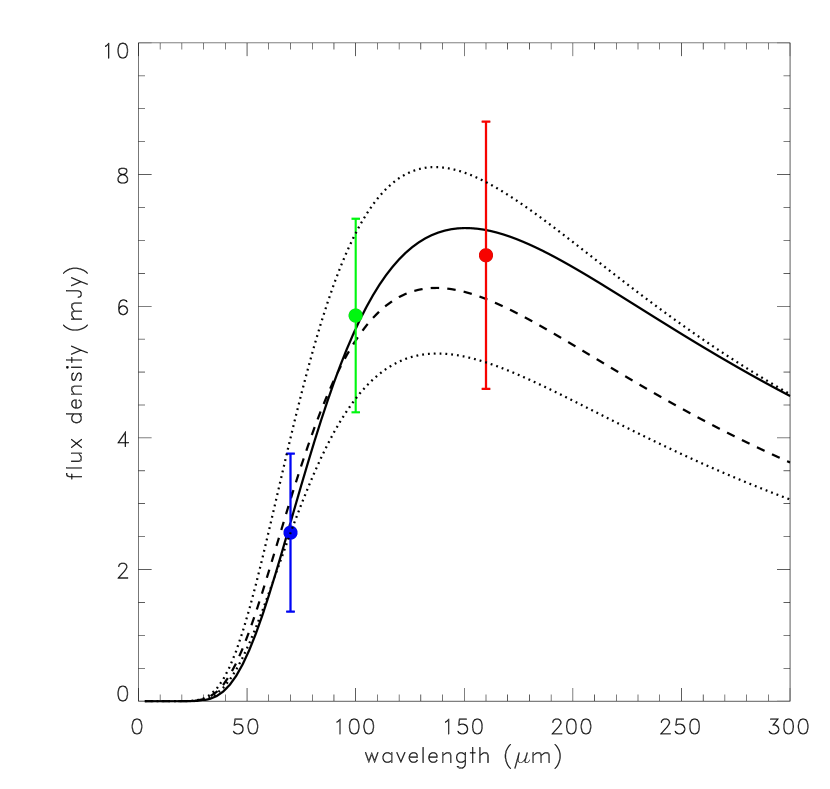
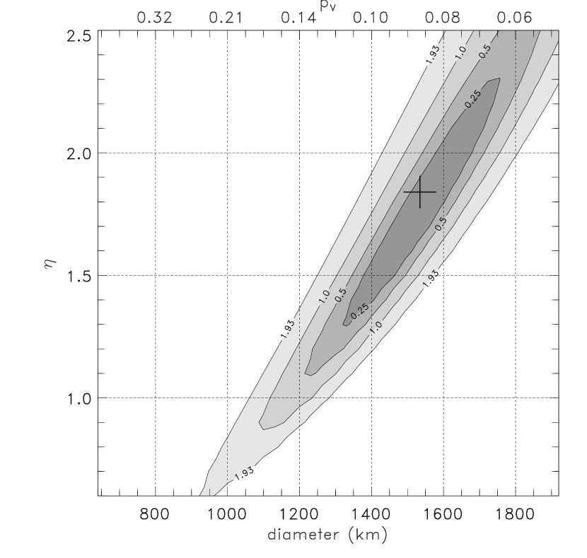
Figure 4.— Left: measured thermal spectral energy distribution of (225088) 2007 OR₁₀, as obtained using Herschel/PACS measurements. The thick black curve shows the best-fit Near-Earth Asteroid Thermal Model (NEATM) curve. The dashed curve represents the best-fit NEATM curve using a fixed beaming parameter of $\eta=1.2$. The two dotted curves correspond to the spectral energy distributions defined by the respective values of diameter and albedo where the value of the reduced $\chi^{2}$ is $1.93$. This value of $1.93$ corresponds to the maximum allowed $\chi^{2}$ for a two degrees-of-freedom fit. Right: contour lines in the reduced $\chi^{2}$ space as the function of the diameter and the beaming parameter in a NEATM fit. The large plus sign marks the position of the best fit thermophysical model solution with the thermal parameters (thermal inertia and surface roughness) converted into beaming parameter.

4. Thermal modelling

Accurate optical photometry has been carried out by Boehnhardt et al. (2014) in order to derive absolute brightness information of several dozens of trans-Neptunian objects which are associated also to the “TNO’s are Cool!” programme. Their reported absolute magnitudes were $H_{\rm V}=2.34\,{\rm mag}$ and $H_{\rm R}=1.49\,{\rm mag}$, however, the formal uncertainties given in this work ($0.01$ mag, in practice, for both $V$ and $R$ colors) are definitely smaller than the amplitude of the detected light curve variations ($0.0444$ mag, see above). Since the rotational phase of this object was unknown at the time of the corresponding VLT/FORS2 observations, we adopted an additional uncertainty in both colors which is equivalent to the amplitude of the light curve variations. Namely, in the subsequent thermal modelling we used $H_{\rm V}=2.34\pm 0.05\,{\rm mag}$ and $H_{\rm R}=1.49\pm 0.05\,{\rm mag}$.

4.1. Near-Earth Asteroid Thermal Model

One of the earliest model capable to the computation of thermal emission of small Solar System bodies is the Standard Thermal Model (STM) by Lebofsky et al. (1986). Basically, this model expects a small phase angle for the object and uses an extrapolation for larger phase angles. However, in the case of 2007 OR₁₀, the phase angle was quite small at the time of Herschel/PACS observations ($0.65^{\circ}$, see also Table 2 for a summary of the observation geometry). Hence, this model yields practically the same results than the sophisticated analysis methods developed for larger phase angles, such as the Near-Earth Asteroid Thermal Model (NEATM) by Harris (1998).

Incorporating STM/NEATM in a fitting procedure allows us to obtain the diameter and geometric albedo of the object by expecting both the thermal fluxes and the absolute magnitude of the object to be known. First, we performed this analysis by involving the aforementioned values of thermal fluxes, absolute magnitudes and a fixed value of the beaming parameter of $\eta=1.2$ (the mean value of beaming parameters derived by Stansberry et al., 2008). We obtained a diameter of $d=1280^{+130}_{-145},{\rm km}$ and $p_{V}=0.125^{+0.033}_{-0.021}$. By letting the beaming parameter $\eta$ to be freely floating during the fit procedure, we got values of $\eta=1.8\pm 0.4$, $d=1550^{+175}_{-190}\,{\rm km}$ and $p_{V}=0.085^{+0.023}_{-0.016}$. We note here that the essential difference between the new estimation presented in this paper and the one found in Santos-Sanz et al. (2012) is the treatment of the beaming parameter. While fixing $\eta=1.2$, these new numbers perfectly agree with that of Santos-Sanz et al. (2012), however, the derived diameter is certainly larger when we consider the beaming parameter as an additional free parameter of this type of thermal model. As we will see later on (in Sec. 4.2), more sophisticated thermophysical models also prefer larger diameters in a nice accordance with NEATM.

The spectral energy distribution as well as the corresponding contour lines in the reduced $\chi^{2}$ space are displayed in Fig. 4. The structure of the contour lines imply a strong correlation between the beaming parameter and the diameter. Due to the lack of a more accurate long wavelength thermal flux at $\lambda=160\,{\rm\mu m}$, the beaming parameter cannot be constrained further (see also the right panel of Fig. 4, where the dashed and solid lines go very close to each other at $\lambda\lesssim 100\,{\rm\mu m}$).

Figure 5.— Left: measured thermal spectral energy distribution of (225088) 2007 OR₁₀, as obtained using Herschel/PACS measurements. The solid curve shows the best-fit TPM model solution corresponding to an equator-on solution while the dashed curve corresponds to the pole-on solution. Middle: the residual flux ratios with respect to the best-fit equator-on TPM solution. Right: The value of the reduced $\chi^{2}$ as the function of the thermal inertia. The decrement in the value of $\chi^{2}$ around $\Gamma\approx 3\,{\rm J}{\rm m}^{-2}{\rm K}^{-1}{\rm s}^{-1/2}$ is clearly visible for the equator-on configuration while there is no such feature for the pole-on geometry. Note that the dashed line shows the $\chi^{2}$ values for $P_{\rm rot}=22.40\,{\rm h}$ in the case of the right panel. See the text for further details about the TPM results for the single-peaked rotational period.

4.2. Thermophysical model

The thermal emission of a trans-Neptunian object can further be characterized by involving the asteroid thermophysical model (TPM, see Lagerros, 1996, 1997, 1998; Müller & Lagerros, 1998, 2002). This model incorporates not only the absolute brightness values and the thermal fluxes but also the rotation period and the orientation geometry of the rotation axis. Throughout our analysis, we tested the possible orientation geometries of pole-on, equator-on and zero obliquity with the respective $(\lambda,\beta)$ polar ecliptic coordinates of $(331.9,-3.3)$; $(331.9,86.7)$ and $(246.8,59.2)$. Our TPM analysis yielded a best-fit solution diameter and albedo close to the results of the NEATM fit with free-floating beaming parameter (see above in Sec. 4.1). Namely, the best-fit TPM parameters for the equator-on geometry and the rotation period of $P_{\rm rot}=44.81\,{\rm h}$ are $d=1535^{+75}_{-225}\,{\rm km}$ and $p_{V}=0.089^{+0.031}_{-0.009}$ while the preferred thermal inertia is $\Gamma=3\,{\rm J}{\rm m}^{-2}{\rm K}^{-1}{\rm s}^{-1/2}$. The spectral energy distribution along with the measured far infrared fluxes (corresponding to these model parameters) are displayed in Fig. 5.

Strictly speaking, we should note that all of the inertia values of $\Gamma\lesssim 20\,{\rm J}{\rm m}^{-2}{\rm K}^{-1}{\rm s}^{-1/2}$ and both equatorial-on and pole-on geometries provide a consistent fit having $\chi^{2}\lesssim 1$. In other words, PACS data do not allow us to constrain the spin-axis orientation, rotation period, thermal inertia or roughness. However, the equator-on, as well as the zero obliquity cases produce more consistent results with reduced $\chi^{2}$ values well below $1.0$, see Fig. 5, right panel. The aforementioned corresponding value for the thermal inertia ($\Gamma=3\,{\rm J}{\rm m}^{-2}{\rm K}^{-1}{\rm s}^{-1/2}$) agrees well with the typical thermal inertias for very distant TNOs (see Lellouch et al., 2013, Fig. 13, right panel) which are roughly in the range of $\Gamma=0.7\dots 5,{\rm J}{\rm m}^{-2}{\rm K}^{-1}{\rm s}^{-1/2}$. Due to the lower confidence of the double-peaked light curve (see Sec. 3), we repeated the TPM analysis for the same set of input parameter with the exception of the rotation period which was fixed to $P_{\rm rot}^{\prime}=22.40\,{\rm h}$. In this case, we obtained $d^{\prime}=1525^{+121}_{-180}\,{\rm km}$ and $p^{\prime}_{V}=0.090^{+0.023}_{-0.013}$ while the preferred thermal inertia is $\Gamma^{\prime}=2\,{\rm J}{\rm m}^{-2}{\rm K}^{-1}{\rm s}^{-1/2}$. These values differs only marginally from the aforementioned values derived for $P_{\rm rot}=44.81\,{\rm h}$. The respective curves are also shown in the plots of Fig. 5.

In order to be able to compare our NEATM and thermophysical model results, the thermal parameters of the best fit thermophysical model solution ($d=1535\,{\rm km}$ for the $P=44.81\,{\rm h}$ rotation period and assuming equator-on geometry) were converted into beaming parameter using the procedure described in Lellouch et al. (2013), based on the papers by Spencer, Lebofsky & Sykes (1989) and Spencer (1990). This conversion resulted in a beaming parameter of $\eta=1.84$ using $\beta=0^{\circ}$ subsolar latitude and a low surface roughness. These best fit diameter and beaming parameter values are in excellent agreement with the best fit values obtained from the NEATM analysis (see also the right panel of Fig. 4).

5. Results and conclusions

Our newly derived diameter of 2007 OR₁₀, $d=1535^{+75}_{-225}\,{\rm km}$ is notably larger than the previously obtained value of Santos-Sanz et al. (2012). This new value would place 2007 OR₁₀ as the third largest dwarf planet – see also Table 3 of Lellouch et al. (2013), after Pluto and Eris. Even considering these refined values, this object is a member of the “bright & red” group of Lacerda et al. (2014).

Due to its large size, 2007 OR₁₀ has likely has a shape close to spherical that may be altered by rotation (see e.g. Lineweaver & Norman, 2010) This should lead to a shape of a MacLaurin spheroid (semimajor axes $a=b>c$, and a rotation around the shortest axis) or to a Jacobi ellipsoid in the case of fast rotation (Plummer, 1919). For a body in hydrostatic equilibrium there is a critical flattening value, $\varepsilon_{\rm crit}=0.42$, when the shape bifurcates from a stable MacLaurin ellipsoid solution to a Jacobi ellipsoid (Plummer, 1919). This critical value would correspond to a rotation period of $P=5.7\,{\rm h}$ assuming a density of $1.2\,{\rm g\,cm^{-3}}$ (a typical value among trans-Neptunian objects, see. e.g. Brown, 2013) and higher densities will make this critical rotation period even shorter. E.g. for a density of $2.5\,{\rm g\,cm^{-3}}$ – a typical value among dwarf planets (Brown, 2008) – the rotation period would just be $3.9\,{\rm h}$ much faster than the rotation period we derived for 2007 OR₁₀.

These critical rotation period values are significantly shorter than either rotation period obtained from K2 observations ($22.40$ or $44.81\,{\rm h}$) in this present paper. This indicates that the rotation curve of 2007 OR₁₀ is very likely due to surface albedo variegations. While the low amplitude variations detected in the light curve of 2007 OR₁₀ can easily be modelled by a single-peaked light curve and small surface brightness inhomogeneities, the two-peaked solution can also be modelled with surface brightness variations with significantly larger amplitudes. In this case, the surface of 2007 OR₁₀ should have areas where the albedo varies between $p_{V}=0.06\dots 0.12$. These limits for the albedo values were derived by fitting a surface albedo distribution characterized by second-order spherical harmonics.

The slow rotation of 2007 OR₁₀ can also be caused by tidal synchronization, similar to the object 2010 WG₉ (see Rabinowitz et al., 2013) and it was also proposed for the objects 2002 GV₃₁ where the slow rotation were first detected also by K2 (see also Pál et al., 2015a). By repeating the similar calculations like what is in Rabinowitz et al. (2013), we can give constraints on the separation of the secondary. These calculations yielded a separation of $\Delta=2.8\times 10^{3}\,{\rm km}$ or $\Delta=4.5\times 10^{3}\,{\rm km}$ for the $\sim 22$ and $\sim 44$ hours or rotation periods, respectively – by expecting two equal-mass bodies with an equivalent effective surface and an average density of $1.5\,{\rm g/cm^{3}}$. At the current distance of 2007 OR₁₀, these separations are equivalent with $0.045^{\prime\prime}$ and $0.071^{\prime\prime}$, respectively. When considering a mass ratio of $8:1$, similar to that of Pluto–Charon system, the separation slightly increases to $\Delta=3.0\times 10^{3}\,{\rm km}$ and $\Delta=4.8\times 10^{3}\,{\rm km}$. Of course, a scenario like the Eris–Dysnomia system can also be feasible with much significant contrast between the surface brightnesses, however, the magnitude of the expected separation is going to be in the same range (see e.g. Sec. 5.3 of Santos-Sanz et al., 2012, for the actual numbers). We note here that according to Kepler’s Third Law, $\Delta\propto(m+M)^{1/3}$, changes in the mass distributions and/or densities affect the separation only slightly.

The red color of 2007 OR₁₀ is likely to be due to the retain of methane, as it was proposed by Brown, Burgasser & Fraser (2011). In Fig. 1 in Brown, Burgasser & Fraser (2011), 2007 OR₁₀ is nearly placed on the retention lines of ${\rm CH}_{4}$, ${\rm CO}$ and ${\rm N}_{2}$. The larger diameter derived in our paper places this dwarf planet further inside the volatile retaining domain, making the explanation of the observed spectrum more feasible.

References

- Balog et al. (2014) Balog, Z. et al. 2014, Exp. Astron., 37, 129
- Benecchi & Sheppard (2013) Benecchi, S. D., Sheppard, S. S. 2013, AJ, 145, 124
- Boehnhardt et al. (2014) Boehnhardt, H.; Schulz, D.; Protopapa, S. & G tz, C. 2014, EM&P, 114, 35
- Borucki et al. (2010) Borucki, W. J., Koch, D., Basri, G., et al. 2010, Science, 327, 977
- Brown (2008) Brown, M. E. 2008, The Solar System Beyond Neptune, M. A. Barucci, H. Boehnhardt, D. P. Cruikshank, and A. Morbidelli (eds.), University of Arizona Press, Tucson, 592 pp., p. 335-344
- Brown, Burgasser & Fraser (2011) Brown, M. E.; Burgasser, A. J. & Fraser, W. C. 2011, ApJ, 738, 26
- Brown (2013) Brown, M. E. 2013, ApJL, 778, 34
- Gilliland et al. (2010) Gilliland, R. L. et al. 2010, ApJL, 713, 160
- Harris (1998) Harris, A. W. 1998 Icarus, 131, 291
- Howell et al. (2014) Howell, S. B., Sobeck, C., Haas, M., et al. 2014, PASP, 126, 398
- Kiss et al. (2014) Kiss, Cs. et al., 2014, ExA, 37, 161
- Kiss et al. (2016) Kiss, Cs. et al., 2016, MNRAS, in press (arXiv:1601.02395)
- Lacerda et al. (2014) Lacerda, P., Fornasier, S., Lellouch, E., et al. 2014, ApJL, 793, 2
- Lagerros (1996) Lagerros, J. S. V., 1996, A&A, 310, 1011
- Lagerros (1997) Lagerros, J. S. V. 1997, A&A, 325, 1226
- Lagerros (1998) Lagerros, J. S. V. 1998, A&A, 332, 1123
- Lebofsky et al. (1986) Lebofsky, L. A., Sykes, M. V., Tedesco, E. F. et al. 1986, Icarus, 68, 239
- Lellouch et al. (2013) Lellouch, E., et al. 2013, A&A, 557, A60
- Lenz & Breger (2005) Lenz P., Breger M., 2005, CoAst, 146, 53
- Lineweaver & Norman (2010) Lineweaver, Ch. & Norman, M. 2010, Proceedings of the 9th Australian Space Science Conference, eds W. Short & I. Cairns, National Space Society of Australia (arXiv:1004.1091)
- Molnár et al. (2015) Molnár, L.; Pál, A.; Plachy, E.; Ripepi, V.; Moretti, M. I.; Szabó, R. & Kiss, L. L. 2015, ApJ, 812, 2
- Monet et al. (2003) Monet, D. G., Levine, S. E.; Canzian, B., et al. 2003, AJ, 125, 984
- Müller & Lagerros (1998) Müller, T. G. & Lagerros, J. S. V. 1998, A&A, 338, 340
- Müller & Lagerros (2002) Müller, T. G. & Lagerros, J. S. V. 2002, A&A, 381, 324
- Müller et al. (2009) Müller, T. G., Lellouch, E, Böhnhardt, H. et al. 2009, EM&P, 105, 209
- Müller, Okumura & Klaas (2011) Müller, Th.G., Okumura, K., Klaas, U.: “PACS Photometer Passbands and Colour Correction Factors for Various Source SEDs”, 2011, PACS internal report, PICC-ME-TN-038, Version 1.0.
- Olling et al. (2015) Olling, R. P. et al., 2015, Nature, 521, 332
- Ott (2010) Ott, S. 2010, in Astronomical Data Analysis Software and Systems XIX. eds. Y. Mizumoto, K.-I. Morita & M. Ohishi, ASP Conf. Ser., 434, 139
- Pál (2012) Pál, A. 2012, MNRAS, 421, 1825
- Pál et al. (2015a) Pál, A.; Szabó, R.; Szabó, Gy. M.; Kiss, L. L.; Molnár, L.; Sárneczky, K. & Kiss, Cs. 2015a, ApJL, 804, 45
- Pál et al. (2015b) Pál, A.; Kiss, Cs.; Horner, J. et al.; 2015b, A&A, in press (arXiv:1507.05468)
- Pilbratt et al. (2010) Pilbratt, G. L. et al., 2010 A&A, 518, 1
- Plummer (1919) Plummer, H. C. 1919, MNRAS, 80, 26
- Poglitsch et al. (2010) Poglitsch, A. et al., 2010, A&A, 518, 2
- Rabinowitz et al. (2013) Rabinowitz, D., Schwamb, M. E., Hadjiyska. E., Tourtellotte, S. & Rojo, P. 2013, AJ, 146, 17
- Santos-Sanz et al. (2012) Santos-Sanz, P.; Lellouch, E.; Fornasier, S. et al. 2012, A&A, 541, 92
- Schwamb et al. (2009) Schwamb, M. E.; Brown, M. E.; Rabinowitz, D. & Marsden, B. G. 2009, Minor Planet Electronic Circ., 2009-A42
- Sheppard (2007) Sheppard, S. S. 2007, AJ, 134, 787
- Spencer, Lebofsky & Sykes (1989) Spencer, J. R.; Lebofsky, L. A. & Sykes, M. V. 1989, Icarus, 78, 337
- Spencer (1990) Spencer, J. R. 1990, Icarus, 83, 27
- Stansberry et al. (2008) Stansberry, J., Grundy, W., Brown, M. et al. 2008, The Solar System Beyond Neptune, M. A. Barucci, H. Boehnhardt, D. P. Cruikshank, and A. Morbidelli (eds.), University of Arizona Press, Tucson, 592 pp., p.161-179
- Szabó et al. (2015) Szabó, R., Sárneczky, K., Szabó, Gy. M., et al. 2015, AJ, 149, 112
- Thompson (2015) Thompson, S. E., 2015, K2 Campaign 3 Data Release Notes, http://keplerscience.arc.nasa.gov/K2/C3drn.shtml