Blind Source Separation: Fundamentals and Recent Advances
(A tutorial overview presented at SBrT-2001)

Abstract

Blind source separation (BSS), i.e., the decoupling of unknown signals that have been mixed in an unknown way, has been a topic of great interest in the signal processing community for the last decade, covering a wide range of applications in such diverse fields as digital communications, pattern recognition, biomedical engineering, and financial data analysis, among others. This course aims at an introduction to the BSS problem via an exposition of well-known and established as well as some more recent approaches to its solution. A unified way is followed in presenting the various results so as to more easily bring out their similarities/differences and emphasize their relative advantages/disadvantages. Only a representative sample of the existing knowledge on BSS will be included in this course. The interested readers are encouraged to consult the list of bibliographical references for more details on this exciting and always active research topic.

1 Introduction

Consider the following scenario. A number of people are found in a room and involved in loud conversations in groups, just as it would happen in a cocktail party. There might also be some background noise, which could be music, car noise from outside, etc. Each person in this room is therefore forced to listen to a mixture of speech sounds coming from various directions, along with some noise. These sounds may come directly to one’s ear or have first suffered a sequence of reverberations because of their reflections on the room’s walls. The problem of focusing one’s listening attention on a particular speaker among this cacophony of conversations and noise has been known as the cocktail party problem [6]. It consists of separating a mixture of speech signals of different characteristics with noise added to it. The signals are a-priori unknown (one listens only to a combination of them) as is also the way they have been mixed. The above scenario is a good analog for many other examples of situations that demand for a separation of mixed signals with no presupposed knowledge on the signals and the system mixing them. The list is long:

• Reception for single- and multi-user communications with no training data [76, 175, 125, 108]

• Analysis of biomedical signals (e.g., electroencephalographic (EEG) [119] and electrocardiographic (ECG) signals [7], fetal electrocardiography [67], functional Magnetic Resonance Imaging (fMRI) data [70], etc.)

• Restoration of images taken from inaccessible scenes [116] (e.g., ultrasonography [1], astronomical imaging [8], images of a nuclear reactor, etc.)

• Feature extraction [11, 105]

• Uncalibrated (or partially calibrated) array processing [22, 25]

• Geophysical exploration [117]

• Denoising [95]

• Voice-controlled machines [172]

• Circuit testing [172]

• Semiconductor manufacturing [172]

• $\cdots$

This kind of problem is commonly referred to as Blind Source Separation (BSS). The term blind is used to emphasize that the signals are to be separated on the basis of their mixture only, without accessing the signals themselves and/or knowing the mixing system, i.e., blindly. Additional information is usually required, involving however only general statistical and/or structural properties of the sources and the mixing mechanism. For example, in a multi-user digital communications system one might assume the signals transmitted to be mutually independent, i.i.d., and BPSK modulated, and the channel(s) to be linear, time-invariant, but otherwise unknown. If no training data are allowed to be transmitted along, due for example to bandwidth limitations, then reception has to be performed blindly.

BSS sounds and is indeed a difficult problem, especially in its most general version. Note that humans experience in general not much difficulty in coping successfully with the cocktail party problem. However, this fact should not be overemphasized, in view of the amazing complexity and performance of the human cognitive system. It would not be that easy to separate speakers talking at the same time by relying, for example, solely on the recordings of a few microphones placed in the room. Nevertheless, a lot of progress has been made in the last ten years or so in the study of the BSS problem and a great number of successful methods, both general and specialized, have been developed and their applicability demonstrated in several contexts. Self-organizing neural networks [83] have, as it will be seen in this course, directly or indirectly played an important role in this research effort, exploiting in a way the human capabilities for BSS through their analogy with related biological mechanisms.

This course aims at providing a tutorial overview of the most important aspects of the BSS problem and approaches to solving it. For reasons to be explained, only methods based on higher-order statistics are discussed. In addition to well-known and established results and algorithms, some more recent developments are also presented that show promise in improving/extending the capabilities and removing the limitations of earlier, classical approaches. BSS is a vast topic, impossible to fit into a short course. Only a selected, yet representative, part of it is thus treated here, hopefully sufficient to motivate interested readers to further explore it with the aid of the (necessarily incomplete) provided bibliography.

The rest of this text is organized as follows. The BSS problem is stated in precise mathematical terms in Section 2, along with a set of assumptions that allow its solution. Section 3 examines the possibility of solving the problem by relying on second-order statistics (SOS) only. It is argued there that SOS are insufficient to provide a piercing solution in all possible scenarios. Higher-order statistics (HOS) are generally required. An elegant and intuitively pleasing manner of expressing and exploiting this additional information is provided by information-theoretic (IT) criteria. Information is defined in Section 4 and its relevance to the BSS problem is explained. The criterion of minimal mutual information (MI) is formulated and interpreted in terms of the Kullback-Leibler divergence. A unification of seemingly unrelated IT and statistical criteria is put forward in Section 5, based on the criterion of minimum MI. This results in a single, “universal” criterion, that is shown to be interpretable in terms of the so-called nonlinear Principal Component Analysis (PCA). A corresponding algorithmic scheme, resulting from its gradient optimization, is presented in Section 6, along with its interpretation as a nonlinear-Hebbian learning scheme and a discussion of the choice of the involved nonlinearities and their implications to algorithm’s stability. It is also shown how the use of the relative gradient in the above algorithm transforms it to one that enjoys the so-called equivariance property. In Section 7 the close relation of the above scheme with the recently proposed FastICA algorithm is demonstrated. The latter is shown in turn to specialize to the super-exponential algorithm, and its variant, the constant-modulus algorithm, well-known from the channel equalization problem. Section 8 discusses algebraic methods for BSS, based on the concept of cumulant tensor diagonalization. Their connection with the above approaches is pointed out, via their interpretation as cost-optimization schemes. Some recently reported deterministic methods, that have been demonstrated to work for short data lengths are also included. The model employed thus far involves a static (memoryless), linear, time-invariant and perfectly invertible mixing system with stationary sources. These simplifying assumptions are relaxed in the following sections. Non-invertible mixing systems are dealt with in Section 9, where both algebraic and criterion-based approaches are discussed. Dynamic (convolutive) mixtures are discussed in Section 10, where methods for dealing with nonlinear or time-varying mixtures and nonstationary sources are also briefly reviewed. Some concluding remarks are included in Section 11.

Notation: Bold lower case and upper case letters will designate vectors and matrices, respectively. Unless stated otherwise, capital, calligraphic, boldface letters will denote higher-order tensors. $\mbox{\boldmath$I$}_{m}$ will be the $m\times m$ identity matrix. The subscript $m$ will be omitted whenever understood from the context. The superscript ^T will denote transposition. $\otimes$ is the Kronecker product. The inverse operation of building a vector from a matrix by stacking its columns one above another will be denoted by ${\rm unvec}(\cdot).$

2 Problem Statement

Consider the mapping

$$\mbox{\boldmath$u$}(n)={\cal F}(\mbox{\boldmath$a$}(n),\mbox{\boldmath$v$}(n),n)$$ (1)

mixing the $N$ source signals

$$\mbox{\boldmath$a$}(n)=\left[\begin{array}[]{cccc}a_{1}(n)&a_{2}(n)&\cdots&a_{N}(n)\end{array}\right]^{T}$$ (2)

and the $K$ noise signals

$$\mbox{\boldmath$v$}(n)=\left[\begin{array}[]{cccc}v_{1}(n)&v_{2}(n)&\cdots&v_{K}(n)\end{array}\right]^{T}$$ (3)

via the mixing system ${\cal F}(\cdot,\cdot,\cdot)$ to yield the mixture

$$\mbox{\boldmath$u$}(n)=\left[\begin{array}[]{cccc}u_{1}(n)&u_{2}(n)&\cdots&u_{M}(n)\end{array}\right]^{T}.$$ (4)

$\cal F$ is in general nonlinear and its time argument, $n$, signifies that it can also be time-varying. BSS can thus be stated as the problem of identifying the mapping $\cal F$ and/or extracting the sources $a$ having access only to the mixture $\mbox{\boldmath$u$}.$ Both the system $\cal F$ and its inputs $\mbox{\boldmath$a$},\mbox{\boldmath$v$}$ are assumed unknown. Nevertheless, so that the problem have a solution, some general structural and/or statistical properties of the quantities involved are assumed. The mixing system is usually supposed to be linear and time-invariant. The most common assumption for the sources is that they are mutually independent and independent of the noise. Depending on the application context, more information may be available. For example, in a digital communications system the source signals might be known to belong to some discrete alphabet. The set of assumptions made for $\cal F$ and $\mbox{\boldmath$a$},\mbox{\boldmath$v$}$ constitute the model adopted for the problem and determine the range of possible solution approaches.

Due to its relative simplicity and wide applicability, the case of a linear, time-invariant mixing system (with stationary sources) has been the focus of the great majority of the works on BSS. This can be written as

$$\mbox{\boldmath$u$}(n)=\mbox{\boldmath$H$}\mbox{\boldmath$a$}(n)+\mbox{\boldmath$v$}(n)$$ (5)

where $H$ is an $M\times N$ mixing matrix and $K=M.$ The following set of assumptions is typical:

• The signals $a_{i}(n)$ and $v_{i}(n)$ are stationary and zero-mean.

• The sources $a_{i}(n)$ are statistically independent.

• The noises $v_{i}(n)$ are statistically independent and independent of the sources.

• The number of sensors exceeds or equals the number of sources: $M\geq N.$

The mixing system in (5) is moreover static, i.e., memoryless. This model could also encompass dynamic systems if it included an assumption of independence between samples of a signal $a_{i}(n)$ and a structural constraint (Toeplitz) on $\mbox{\boldmath$H$}.$ Linear systems with memory will be briefly addressed in Section 10.

The goal of the linear BSS is to determine a separating matrix $G$ such that

$$\mbox{\boldmath$y$}(n)=\mbox{\boldmath$G$}\mbox{\boldmath$u$}(n)$$ (6)

is a good approximation of the source signals. Assumption A4 signifies that the mixture is not under-determined, i.e., in the absence of noise, if $H$ is identified and of full rank, then it can be inverted to yield the sources. If noise is not weak enough to be neglected, perfect recovery of all sources is impossible. In fact, the noisy mixture may be viewed as a special case of a noise-free mixture that does not meet A4. Just write (5) in the form

$$\mbox{\boldmath$u$}(n)=\mbox{\boldmath$H$}^{\prime}\mbox{\boldmath$a$}^{\prime}(n)$$

where $\mbox{\boldmath$H$}^{\prime}=\left[\begin{array}[]{cc}\mbox{\boldmath$H$}&\mbox{\boldmath$I$}_{M}\end{array}\right]$ and $\mbox{\boldmath$a$}^{\prime}(n)=\left[\begin{array}[]{cc}\mbox{\boldmath$a$}^{T}(n)&\mbox{\boldmath$v$}^{T}(n)\end{array}\right]^{T}.$ Then $\mbox{\boldmath$H$}^{\prime}$ is $M\times(M+N)$ and cannot be (linearly) inverted. Hence, one can, without loss of generality, write

$$\mbox{\boldmath$u$}(n)=\mbox{\boldmath$H$}\mbox{\boldmath$a$}(n)$$ (7)

for the linear mixing process. The general linear BSS setup is shown schematically in Fig. 1.

Figure 1: Linear BSS setup.

The (nonlinear) function $\mbox{\boldmath$g$}(\cdot)$ at the separator’s output may not be really there. It is needed however in the development of the criteria and associated algorithms.

It must be noted that, unless additional information is available, there is an indeterminacy with respect to the scaling and order of the separated sources [172]. The result of the mixing in (7) will not change if a source is multiplied with a scalar and the corresponding column of $H$ is divided by it. A permutation of the source signals accompanied by an analogous permutation of the columns of the mixing matrix will not have any effect on $\mbox{\boldmath$u$}(n)$ either. The best one could expect therefore is to recover $a_{i}$’s scaled and/or permuted, i.e.,

$$\mbox{\boldmath$y$}(n)=\mbox{\boldmath$P$}\mbox{\boldmath$D$}\mbox{\boldmath$a$}(n)$$

where $P$ is a permutation matrix and $D$ is a diagonal (invertible) matrix. The following assumption on the source energy can therefore be made without harming the generality:

• The sources have unit variance: $E[|a_{i}(n)|^{2}]=1.$

This course, in its main part, will focus on the noise-free, linear, static (instantaneous) mixture case (7), with as many sensors as sources, i.e., $M=N$, an invertible mixing matrix, and sources satisfying assumptions A1, A2, A5. Furthermore, to simplify the presentation, we shall frequently omit the inherent scale and order indeterminacy and write $\mbox{\boldmath$G$}=\mbox{\boldmath$H$}^{-1}.$ Moreover, all quantities are assumed to be real. It will be usually straightforward to extend the results to the complex case.

The model adopted may not be realistic in many practical scenarios. It is sufficient however to convey the basic ideas underlying the problem, while keeping things simple. Besides, as the following analysis should show, its study is already far from being trivial.

3 Are Second-Order-Statistics Sufficient?

Based on the model assumptions made above, the BSS problem is solved once the mixing matrix $H$ has been identified. Thus the question arises whether $H$ could be somehow extracted from measuring appropriate quantities related to the mixture signals. Note that the autocorrelation matrix of the observation vector $\mbox{\boldmath$u$}(n)$ is given by:

$$\mbox{\boldmath$R$}_{u}=E[\mbox{\boldmath$u$}(n)\mbox{\boldmath$u$}^{T}(n)]=\mbox{\boldmath$H$}\mbox{\boldmath$R$}_{a}\mbox{\boldmath$H$}^{T}=\mbox{\boldmath$H$}\mbox{\boldmath$H$}^{T}$$ (8)

where the index $n$ is omitted due to stationarity and the source autocorrelation matrix $\mbox{\boldmath$R$}_{a}=E[\mbox{\boldmath$a$}(n)\mbox{\boldmath$a$}^{T}(n)]$ equals the identity according to the assumptions A1, A2, and A5. The above equation suggests that the mixing matrix might be identifiable as a square root of $\mbox{\boldmath$R$}_{u},$ i.e., $\mbox{\boldmath$H$}=\mbox{\boldmath$R$}_{u}^{1/2}$, via its eigenvalue decomposition (EVD) for example. In fact it is only a basis for the column space of $H$ that this would provide. It is easy to see that not only $H$ but also any product of it with an orthogonal matrix, $\mbox{\boldmath$H$}\mbox{\boldmath$Q$}^{T}$, will verify (8). In other words, $\mbox{\boldmath$R$}_{u}$ allows $H$ to be identified only up to an orthogonal factor, $\mbox{\boldmath$Q$}^{T}$.

It is instructive to observe that this ambiguity is an instance of the well-known phase indeterminacy problem in spectral factorization for linear prediction [143], where the role of the sources play the innovation sequence samples. The net effect of the corresponding “separator” $\mbox{\boldmath$T$}=\mbox{\boldmath$R$}_{u}^{-1/2}$ is to whiten the observations:

$$\mbox{\boldmath$\bar{u}$}(n)=\mbox{\boldmath$T$}\mbox{\boldmath$u$}(n)$$ (9)

with

$$\mbox{\boldmath$R$}_{\bar{u}}=\mbox{\boldmath$T$}\mbox{\boldmath$R$}_{u}\mbox{\boldmath$T$}^{T}=\mbox{\boldmath$I$}_{N}.$$

The operation (9) amounts to a projection of the available data $\mbox{\boldmath$u$}(n)$ onto the principal directions determined from $\mbox{\boldmath$R$}_{u}$ and is known in the statistics jargon as Principal Component Analysis (PCA) [58, 78]. The whitened vector $\mbox{\boldmath$\bar{u}$}(n)$, whose entries are the principal components of $\mbox{\boldmath$u$}(n)$, is commonly referred to as standardized or sphered [117, 55].

The above reduces the original problem to one where the mixing matrix is constrained to be orthogonal:

$$\mbox{\boldmath$\bar{u}$}(n)=\mbox{\boldmath$T$}\mbox{\boldmath$H$}\mbox{\boldmath$a$}(n)=\mbox{\boldmath$Q$}\mbox{\boldmath$a$}(n),\mbox{\ \ }\mbox{\boldmath$Q$}\mbox{\boldmath$Q$}^{T}=\mbox{\boldmath$I$}.$$ (10)

It is clear that to eliminate the remaining uncertainty about $H$ more information is required. In fact it turns out that, subject to some hypotheses on the source signals to be described shortly, the mixing matrix can be identified by exploiting the mixture autocorrelation for a nonzero lag as well. Assume that there is a lag $k\neq 0$ for which no two sources have the same autocorrelation, i.e.,

$$E[a_{i}(n)a_{i}(n-k)]\neq E[a_{j}(n)a_{j}(n-k)],\mbox{\ for all\ }i\neq j.$$ (11)

Take the lag-$k$ autocorrelation matrix of the standardized data:

$$\mbox{\boldmath$R$}_{\bar{u}}(k)=E[\mbox{\boldmath$\bar{u}$}(n)\mbox{\boldmath$\bar{u}$}^{T}(n-k)]=\mbox{\boldmath$Q$}\mbox{\boldmath$R$}_{a}(k)\mbox{\boldmath$Q$}^{T}.$$ (12)

By A2 $\mbox{\boldmath$R$}_{a}(k)$ is diagonal, hence the above equation represents an EVD of $\mbox{\boldmath$R$}_{\bar{u}}(k).$ In view of (11), the eigenvalues $E[a_{i}(n)a_{i}(n-k)]$ are distinct. This implies that the columns of $Q$ are uniquely determined from an EVD of $\mbox{\boldmath$R$}_{\bar{u}}(k)$ subject to sign/order changes.

The above method, known as Algorithm for Multiple Unknown Signals Extraction (AMUSE) [172], is found at the heart of many other BSS algorithms relying on the mixture’s SOS. These approaches provide simple and fast BSS tools whose effectiveness is well documented in the relevant literature [172]. They rely heavily however on the assumption that not two sources have the same power spectral contents (see (11)). If two sources have different, but similar, power spectra, the separation will be theoretically possible but with practically unreliable results [117]. Moreover, it is clear that these methods will not apply to scenarios where $a_{i}(n)$ should be considered as white, and even i.i.d.

Since it is our purpose to cover methods for the BSS problem in its generality as described in Section 2, no assumption like (11) will be made henceforth. It is then made clear from the above discussion that (10) represents the limit of what a SOS-based approach can bring to our problem. In fact, one cannot go any further than that in the case that sources are Gaussian, since such a signal is completely described by its mean and covariance. It will be shown later on that at most one source can be Gaussian if the BSS problem is to have any solution at all. Observe that in the above algorithm the sources did not have to be independent, only the fact that they are uncorrelated was made use of. This suggests that confining ourselves to the second-order information does not exploit all available knowledge. It is of interest to recall that it is for a Gaussian signal that the notions of independence and uncorrelatedness coincide [143]. However, most of the sources encountered in practical applications, e.g., speech, music, data, image, are distinctly non-Gaussian. It follows therefore that another transformation, that can extract from the data more structure than PCA is able to, is needed. This will be what we call Independent Component Analysis (ICA).

4 Mutual Information and Independent Component Analysis

4.1 Statistical Independence

The independence assumption for the source signals can be equivalently stated as the equality of the joint probability density function (pdf) of the source vector $\mbox{\boldmath$a$}(n)$ with the product of the marginal pdf’s of its entries:

$$p_{a}(\mbox{\boldmath$a$})=\tilde{p}_{a}(\mbox{\boldmath$a$})\stackrel{{\scriptstyle\triangle}}{{=}}\prod_{i=1}^{N}p_{a_{i}}(a_{i}).$$ (13)

Hence an analogous equality would hold for the output of a successful separating system, i.e.,

$$p_{y}(\mbox{\boldmath$y$})=\tilde{p}_{y}(\mbox{\boldmath$y$})\stackrel{{\scriptstyle\triangle}}{{=}}\prod_{i=1}^{N}p_{y_{i}}(y_{i}).$$ (14)

The above represents the goal of the ICA transformation, i.e., (linearly) transforming a random vector into one with (as) independent components (as possible). Information theory constitutes a powerful and elegant framework for expressing and studying this problem.

4.2 Entropy and Mutual Information

Recall that the entropy of a random variable provides a measure of our uncertainty about the value this variable takes. For a continuous-valued random vector $x$, it takes the form [143, 91]

$$H(\mbox{\boldmath$x$})=-E[\ln p_{x}(\mbox{\boldmath$x$})]=-\int p_{x}(\mbox{\boldmath$x$})\ln p_{x}(\mbox{\boldmath$x$})d\mbox{\boldmath$x$}.$$ (15)

In fact this is rather what we call the differential entropy of $x$. The entropy of a continuous random vector goes to infinity (since the uncertainty on the value assumed is infinite) and is equal to the differential entropy only modulo a reference term [91]. However, since it will be the optimization of such quantities and mainly their differences that will be interested in, we may rest on the differential entropy and call it simply entropy from now on.

$H(\mbox{\boldmath$x$})$ is a measure of the uncertainty on the value of the vector $\mbox{\boldmath$x$}.$ Let another random vector $y$, and let $p_{x|y}(\mbox{\boldmath$x$}|\mbox{\boldmath$y$})$ denote the pdf of $x$ conditioned on $\mbox{\boldmath$y$}.$ Then a measure of the uncertainty remaining about $x$ after having observed $y$ can be given by the conditional entropy:

$$H(\mbox{\boldmath$x$}|\mbox{\boldmath$y$})=-E[\ln p_{x|y}(\mbox{\boldmath$x$}|\mbox{\boldmath$y$})]=-\int p_{x,y}(\mbox{\boldmath$x$},\mbox{\boldmath$y$})\ln p_{x|y}(\mbox{\boldmath$x$}|\mbox{\boldmath$y$})d\mbox{\boldmath$x$}d\mbox{\boldmath$y$}$$ (16)

where

$$p_{x,y}(\mbox{\boldmath$x$},\mbox{\boldmath$y$})=p_{x|y}(\mbox{\boldmath$x$}|\mbox{\boldmath$y$})p_{y}(\mbox{\boldmath$y$})$$ (17)

is the joint pdf of $x$ and $\mbox{\boldmath$y$}.$ It is then reasonable to say that the difference

$$I(\mbox{\boldmath$x$},\mbox{\boldmath$y$})=H(\mbox{\boldmath$x$})-H(\mbox{\boldmath$x$}|\mbox{\boldmath$y$})$$ (18)

represents the information concerning $x$ that is acquired when observing $\mbox{\boldmath$y$}.$ It is termed as the mutual information (MI) between $x$ and $\mbox{\boldmath$y$}.$ As it will be seen shortly, $I(\mbox{\boldmath$x$},\mbox{\boldmath$y$})$ is always nonnegative and vanishes if and only if $x$ and $y$ are statistically independent. This is to be expected since for independent $x$ and $y$ the observation of the one does not provide any information concerning the other. This is also seen in the definition (18) since then $H(\mbox{\boldmath$x$}|\mbox{\boldmath$y$})=H(\mbox{\boldmath$x$}).$ The MI is thus a meaningful measure of statistical dependence and, in fact, it will prove to be a good starting point for a fruitful study of ICA.

4.3 Kullback-Leibler Divergence

The condition for independence stated in (14) implies that independence can also be viewed in terms of the distance between $p_{y}(\mbox{\boldmath$y$})$ and $\tilde{p}_{y}(\mbox{\boldmath$y$}).$ A measure of closeness between two pdf’s $p_{x}$ and $p_{y}$ is given by the so-called Kullback-Leibler divergence (KLD), defined as [91]

$$D(p_{x}\|p_{y})=E_{x}\left[\ln\frac{p_{x}(\mbox{\boldmath$r$})}{p_{y}(\mbox{\boldmath$r$})}\right]=\int p_{x}(\mbox{\boldmath$r$})\ln\frac{p_{x}(\mbox{\boldmath$r$})}{p_{y}(\mbox{\boldmath$r$})}d\mbox{\boldmath$r$}.$$ (19)

An important property of the KLD is that it is always nonnegative and becomes zero if and only if its two arguments coincide. Hence, although it is not symmetric with respect to its arguments, it is employed as a metric for the space of pdf’s. The KLD satisfies (under some weak conditions [91]) the following relationship, where $p_{x},p_{y},p_{z}$ are pdf’s:

$$D(p_{x}\|p_{y})=D(p_{x}\|p_{z})+D(p_{z}\|p_{y}).$$ (20)

This can be viewed as the extension of the Pythagorean theorem for orthogonal triangles in Euclidean spaces to the space of pdf’s endowed with the metric $D(\cdot\|\cdot)$ and will be seen below to provide a means for an insightful analysis of BSS criteria.

Another property of the KLD that is going to be used in the sequel is that it is invariant under any invertible (linear or nonlinear) transformation, i.e., for any $\mbox{\boldmath$g$}(\cdot)$,

$$D(p_{g(x)}\|p_{g(y)})=D(p_{x}\|p_{y}).$$ (21)

The MI between $x$ and $y$ can be formulated as a KLD. Indeed, using eqs. (15), (16), (17) in (18) results in

$$I(\mbox{\boldmath$x$},\mbox{\boldmath$y$}) = \int p_{x,y}(\mbox{\boldmath$x$},\mbox{\boldmath$y$})\ln\frac{p_{x,y}(\mbox{\boldmath$x$},\mbox{\boldmath$y$})}{p_{x}(\mbox{\boldmath$x$})p_{y}(\mbox{\boldmath$y$})}\,d\mbox{\boldmath$x$}d\mbox{\boldmath$y$}$$ (22)

$$= D(p_{x,y}\|p_{x}p_{y})$$

verifying the appropriateness of the MI as a measure of statistical dependence.

The KLD formulation above makes easier to also define the mutual information between the entries of an $N$-vector, $\mbox{\boldmath$y$}.$ It will simply equal the KLD between $p_{y}(\mbox{\boldmath$y$})$ and $\tilde{p}_{y}(\mbox{\boldmath$y$})$ in (14):

$$I(\mbox{\boldmath$y$})=D(p_{y}\|\tilde{p}_{y})=\int\int\cdots\int p_{y}(y_{1},y_{2},\ldots,y_{N})\ln\frac{p_{y}(y_{1},y_{2},\ldots,y_{N})}{\prod_{i=1}^{N}p_{y_{i}}(y_{i})}\,dy_{1}dy_{2}\cdots dy_{N}$$ (23)

and vanish if and only if the components of $y$ are mutually independent. From the above equation an expression of $I(\mbox{\boldmath$y$})$ in terms of the entropy of $y$ and the (marginal) entropies of its entries readily results:

$$I(\mbox{\boldmath$y$})=-H(\mbox{\boldmath$y$})+\sum_{i=1}^{N}H(y_{i}).$$ (24)

Thus, minimizing MI amounts to making the entropy of $y$ as close as possible to the sum of its marginal entropies.

Negentropy, the distance of a given pdf from the Gaussian pdf with the same mean and covariance, can also be defined with the aid of the KLD as

$$J_{G}(\mbox{\boldmath$y$})\stackrel{{\scriptstyle\triangle}}{{=}}D(p_{y}\|p_{y^{G}}),$$ (25)

where $\mbox{\boldmath$y$}^{G}$ denotes a Gaussian random vector with the same mean and covariance as $\mbox{\boldmath$y$}.$

4.4 Negative Mutual Information as an ICA Contrast

It will be useful to write the MI of the vector $y$ in terms of its negentropy. This is easily done by appealing to the Pythagorean theorem for KLD’s [35]. Just write (20) for the two triangles shown in Fig. 2.

Figure 2: Information-geometric interpretation of the relation between mutual information and negentropy [35].

This yields:

$$D\left(p_{y}\|\prod_{i=1}^{N}p_{y_{i}^{G}}\right) = D(p_{y}\|p_{y^{G}})+D\left(p_{y^{G}}\|\prod_{i=1}^{N}p_{y_{i}^{G}}\right)$$

$$= J_{G}(\mbox{\boldmath$y$})+I_{G}(\mbox{\boldmath$y$})$$

and

$$D\left(p_{y}\|\prod_{i=1}^{N}p_{y_{i}^{G}}\right) = D\left(p_{y}\|\prod_{i=1}^{N}p_{y_{i}}\right)+D\left(\prod_{i=1}^{N}p_{y_{i}}\|\prod_{i=1}^{N}p_{y_{i}^{G}}\right)$$

$$= I(\mbox{\boldmath$y$})+\sum_{i=1}^{N}J_{G}(y_{i}),$$

with $I_{G}(\mbox{\boldmath$y$})$ denoting the MI of the Gaussian version of $y$, $\mbox{\boldmath$y$}^{G}.$ It then follows that

$$I(\mbox{\boldmath$y$})=I_{G}(\mbox{\boldmath$y$})+\left(J_{G}(\mbox{\boldmath$y$})-\sum_{i=1}^{N}J_{G}(y_{i})\right).$$ (26)

The above shows $I(\mbox{\boldmath$y$})$ to consist of two terms responsible for the redundancy within $p_{y}$. The first term accounts for the second-order information in the process $y$, whereas non-Gaussian, higher-order information is measured by the second term. The prewhitening transformation discussed in Section 2 aims at nulling $I_{G}(\mbox{\boldmath$y$})$. Methods based on higher-order statistics can then be employed to minimize the second term, subject to the constraint that the separating matrix be orthogonal. It should be emphasized that this two-step minimization of the MI is not necessarily optimal [35]. Ideally, the function in (26) should be optimized as a whole. Such approaches have only recently been reported [37, 124, 166]. It is however a common practice to first sphere the data before going on to extract their higher-order structure. An advantage of such an approach is that the corresponding normalization of the data may help avoid numerical inaccuracies that could result from the subsequent nonlinear operations [117]. Moreover, the fact that the separating matrix is then orthogonal may sometimes facilitate the derivation of separation methods [48, 138]. Bounds on the errors in the separation due to imperfect standardization have been derived and reported in [26]. In general, the standardization step poses no problem for the separation task (provided of course one uses a sufficiently large number of samples to estimate the autocorrelation matrix) and two-step methods have proved their effectiveness in practice [117].

It was seen above that the MI is a meaningful measure of statistical dependence. In fact, its minimization constitutes a valid criterion for BSS, since it can be shown that $\psi(p_{y})=-I(\mbox{\boldmath$y$})$ is a contrast over the set of random $N$-vectors [48]. A real-valued function, $\Psi$, defined on the space of $N$-variate pdf’s, is said to be a contrast if it satisfies the following requirements:

• $\Psi(p_{y})$ is invariant to permutations:

  $$\Psi(p_{Py})=\Psi(p_{y})\mbox{\ for any permutation matrix\ }\mbox{\boldmath$P$}$$

• $\Psi(p_{y})$ is invariant to scale changes:

  $$\Psi(p_{Dy})=\Psi(p_{y})\mbox{\ for any diagonal matrix\ }\mbox{\boldmath$D$}$$

• If $y$ has independent components, then

  $$\Psi(p_{Ay})\leq\Psi(p_{y}),\mbox{\ for any invertible matrix\ }\mbox{\boldmath$A$}.$$

Requirement C3 shows that the ICA might be obtained by maximizing a contrast of the separator’s output $\mbox{\boldmath$y$}.$ The requirements C1, C2 correspond to the permutation/scaling indeterminacy inherent in the BSS problem, as discussed in Section 2. However, there is one more requirement that a contrast should satisfy so that it can be a valid BSS cost functional:

• The equality in C3 holds if and only if $A$ is a generalized permutation matrix, i.e., $\mbox{\boldmath$A$}=\mbox{\boldmath$P$}\mbox{\boldmath$D$}$, where $P$ is a permutation matrix and $D$ is an invertible diagonal matrix.

A contrast satisfying C4 as well is said to be discriminating. It can be shown that the negative MI, $\psi_{ICA}(p_{y})\stackrel{{\scriptstyle\triangle}}{{=}}-I(\mbox{\boldmath$y$})$, is a discriminating contrast over all $N$-vectors $y$ with at most one Gaussian component [48]. Henceforth, the term contrast will be used to refer to a discriminating contrast.

Before concluding this section, let us consider simplifying the expression for the negative MI contrast. Taking into account the fact that the separating matrix $G$ is invertible, one can express the joint pdf of $y$ in (6) in terms of that of $u$ using the well-known formula [143]:

$$p_{y}(\mbox{\boldmath$y$})=\frac{p_{u}(\mbox{\boldmath$G$}^{-1}\mbox{\boldmath$y$})}{|\det(\mbox{\boldmath$G$})|}.$$ (27)

This in turn allows the entropy of $y$ to be expressed in terms of that of $u$:

$$H(\mbox{\boldmath$y$})=H(\mbox{\boldmath$u$})+\ln|\det(\mbox{\boldmath$G$})|.$$ (28)

Thus (24) becomes

$$I(\mbox{\boldmath$y$})=-H(\mbox{\boldmath$u$})-\ln|\det(\mbox{\boldmath$G$})|-E_{y}\left[\ln\prod_{i=1}^{N}p_{y_{i}}(y_{i})\right]$$

Since $H(\mbox{\boldmath$u$})$ does not depend on $G$, the corresponding contrast may be written as

$$\psi_{ICA}(\mbox{\boldmath$G$})=\ln|\det(\mbox{\boldmath$G$})|+E_{y}\left[\ln\prod_{i=1}^{N}p_{y_{i}}(y_{i})\right],$$ (29)

where, to emphasize its role in BSS, the dependence on $G$ is made explicit. The role of the first term above is to ensure a valid separation solution, with $G$ invertible. Note that with prewhitened mixture data, $G$ is orthogonal and the first term becomes zero. The maximization of $\psi_{ICA}$ amounts then to minimizing the sum of the entropies of the components of $\mbox{\boldmath$y$}.$ Since maximum entropy corresponds to Gaussianity [143, 91], this is equivalent to making the $y_{i}$’s as less Gaussian as possible, which necessarily involves statistics of order higher than two. The central limit theorem [143] provides another interpretation of that, since a linear mixture of independent signals tends to be close to Gaussian. This minimum-entropy, or minimum Gaussianity point of view has been central in pioneering works on blind deconvolution [14, 71] and will be further elaborated upon later on.

5 A “Universal” Criterion for BSS

It will be of interest to examine the possible connections between the minimum MI criterion and other proposed criteria that are inspired from information theory and statistics. It will be seen that subject to some constraints on the choice of the nonlinearities involved, all these criteria are equivalent and can thus be viewed as special cases of a single, “universal” criterion.

5.1 Infomax and MaxEnt

We have seen above that sources are completely separated when the separator’s outputs are independent or equivalently their mutual information is zero. An alternative way of looking at the separation goal is by formulating it as a maximal information transfer from the mixture, $u$, to the source estimates, $y$ [9]. This criterion, similar to the principle of information rate and capacity in the Shannon theory of communication, though less evidently pertinent to the BSS task, will be seen to be closely related to that of minimum MI between the entries of $\mbox{\boldmath$y$}.$

Consider the MI between $u$ and $y$, namely:

$$I(\mbox{\boldmath$y$},\mbox{\boldmath$u$})=H(\mbox{\boldmath$y$})-H(\mbox{\boldmath$y$}|\mbox{\boldmath$u$}).$$

Since the transfer from $u$ to $y$ is deterministic, knowledge of the first completely determines the latter, hence the second term above is null. Therefore, in this context:

$$I(\mbox{\boldmath$y$},\mbox{\boldmath$u$})=H(\mbox{\boldmath$y$}).$$ (30)

Since for an unrestricted $y$ its entropy has no bound, we assume an entrywise nonlinearity at the output of the separating system $G$ (see Fig. 1), i.e.,

$$\mbox{\boldmath$y$}(n)=\mbox{\boldmath$g$}(\mbox{\boldmath$G$}\mbox{\boldmath$u$}(n))$$ (31)

where

$$\mbox{\boldmath$g$}(x)\stackrel{{\scriptstyle\triangle}}{{=}}\left[\begin{array}[]{cccc}g_{1}(x_{1})&g_{2}(x_{2})&\cdots&g_{N}(x_{N})\end{array}\right]^{T}$$

and the functions $g_{i}$ are monotonically increasing with $g_{i}(-\infty)=0$ and $g_{i}(\infty)=1$. These are the common assumptions for the nonlinearities in artificial neural networks (ANN) [91]. Then the entropy of $y$ is maximized when $p_{y}(\mbox{\boldmath$y$})$ equals $U_{N}(\mbox{\boldmath$y$})$, the uniform pdf in $[0,1]^{N}.$ Note that in that case, the components of $y$ are statistically independent and uniformly distributed in $[0,1]$. If $g_{i}$ is chosen to be equal to the cumulative distribution function (cdf) of the source $i$, $p_{y_{i}}(y_{i})$ can only be uniform in $[0,1]$ when $y_{i}$ is equal to $a_{i}$ or to another source having the same pdf. Therefore the maximization of the entropy of $y$ yields a meaningful criterion for BSS, called MaxEnt [10]. In view of (30), this criterion is equivalent to the maximization of the MI $I(\mbox{\boldmath$y$},\mbox{\boldmath$u$})$, referred to as Infomax [10, 9]. The above source-output pdf-matching point of view was also considered in early studies of blind equalization [14] and will be seen to underly the maximum likelihood approach as well.

The MaxEnt and Infomax criteria can be seen to be equivalent, under some conditions, with the minimum MI criterion discussed in Section 4. This equivalence has been argued upon in [10] considering the functions $g_{i}$ as being given by the source pdf’s, as explained above. However, a more rigorous study was reported in [185] and [137]. Here a brief explanation of this relation will be provided stating more subtle results without proof. Denote by $x$ the linear part of the separating system (see Fig. 1), i.e.,

$$\mbox{\boldmath$x$}(n)=\mbox{\boldmath$G$}\mbox{\boldmath$u$}(n).$$ (32)

Then, since $\mbox{\boldmath$g$}(\cdot)$ is invertible it holds that [143]

$$p_{y}(\mbox{\boldmath$y$})=\frac{p_{x}(\mbox{\boldmath$x$})}{\left|\prod_{i=1}^{N}g_{i}^{\prime}(x_{i})\right|},$$

with $g_{i}^{\prime}$ denoting the first derivative of $g_{i}.$ The entropy of $y$ can thus be written as

$$H(\mbox{\boldmath$y$})=H(\mbox{\boldmath$u$})+\ln|\det(\mbox{\boldmath$G$})|+E_{x}\left[\ln\prod_{i=1}^{N}g_{i}^{\prime}(x_{i})\right].$$ (33)

Hence the Infomax (IM), or equivalently MaxEnt, criterion reads as:

$$\max_{G}\left(\psi_{IM}(\mbox{\boldmath$G$})\stackrel{{\scriptstyle\triangle}}{{=}}\ln|\det(\mbox{\boldmath$G$})|+E_{x}\left[\ln\prod_{i=1}^{N}g_{i}^{\prime}(x_{i})\right]\right).$$ (34)

Comparing eqs. (29) and (34), one can see that these two criteria are equivalent if $g_{i}$’s coincide with source cdf’s. Eq. (26) expresses the MI between the components of $y$ in terms of its joint and marginal negentropies. It has been demonstrated that Infomax is also equivalent with negentropy maximization, under the same conditions [121]. In fact, since it is the stability of the desired stationary point $\mbox{\boldmath$G$}=\mbox{\boldmath$H$}^{-1}$ that counts, it can be seen that a mismatch between the $g_{i}$’s and the source probability laws can be tolerated. This is stated in [137] as a requirement for sufficiently rich parameterization of $g_{i}$. The problem of correctly choosing the nonlinearities $g_{i}$ will be discussed in more detail later on when dealing with the corresponding algorithms.

5.2 Maximum Likelihood and Bayesian Approaches

Let us continue to consider the demixing model $\mbox{\boldmath$y$}=\mbox{\boldmath$g$}(\mbox{\boldmath$x$})$ where the $g_{i}$’s are always taking values in $[0,1].$ Then the entropy of $y$ can be written as the negative distance of its pdf from the uniform one:

$$H(\mbox{\boldmath$y$}) = -\int p_{y}(\mbox{\boldmath$y$})\ln\left[\frac{p_{y}(\mbox{\boldmath$y$})}{\prod_{i=1}^{N}U(y_{i})}\right]d\mbox{\boldmath$y$}$$ (35)

$$= -D(p_{y}\|U_{N}),$$

where $U(y_{i})$ is the uniform pdf in $[0,1]$ and $U_{N}(\mbox{\boldmath$y$})=\prod_{i=1}^{N}U(y_{i}).$ In order to formulate a Maximum Likelihood (ML) approach to the corresponding BSS problem, we need a model for the observed data generation including a hypothesis for the source statistics. According to (7) this will be written as

$$\mbox{\boldmath$u$}=\mbox{\boldmath$\Theta$}\mbox{\boldmath$\tilde{a}$}$$

where ideally $\mbox{\boldmath$\Theta$}=\mbox{\boldmath$H$}$ and $\mbox{\boldmath$\tilde{a}$}=\mbox{\boldmath$a$}.$ Parameterize the pdf of $u$ as $p_{u}(\mbox{\boldmath$u$}|\mbox{\boldmath$\Theta$}).$ Although this pdf depends on both the system parameter and our hypothesized probability model for the sources, $\tilde{a}$, the latter will be omitted from this notation since it will be with respect to $\Theta$ that the criterion will be optimized. The idea in the ML principle is to find, among a set of choices for $\Theta$, that which maximizes the pdf of the data conditioned on the model parameter.

Take $T$ independent realizations of $u$, say, $\mbox{\boldmath$u$}(1),\ldots,\mbox{\boldmath$u$}(T).$ Then the likelihood that these samples are drawn with a pdf $p_{u}(\mbox{\boldmath$u$}|\mbox{\boldmath$\Theta$})$ is given by $\prod_{t=1}^{T}p_{u}(\mbox{\boldmath$u$}(t)|\mbox{\boldmath$\Theta$}).$ The normalized log-likelihood will be

$$L_{T}(\mbox{\boldmath$\Theta$})=\frac{1}{T}\ln\prod_{t=1}^{T}p_{u}(\mbox{\boldmath$u$}(t)|\mbox{\boldmath$\Theta$})=\frac{1}{T}\sum_{t=1}^{T}\ln p_{u}(\mbox{\boldmath$u$}(t)|\mbox{\boldmath$\Theta$}).$$

As in (27), we have

$$p_{u}(\mbox{\boldmath$u$}(t)|\mbox{\boldmath$\Theta$}) = \frac{p_{\tilde{a}}(\mbox{\boldmath$\Theta$}^{-1}\mbox{\boldmath$u$}(t))}{|\det(\mbox{\boldmath$\Theta$})|}$$

$$= p_{\tilde{a}}(\mbox{\boldmath$x$}(t))|\det(\mbox{\boldmath$G$})|$$

where we recall that $\mbox{\boldmath$x$}=\mbox{\boldmath$G$}\mbox{\boldmath$u$}$ and we set $\mbox{\boldmath$G$}=\mbox{\boldmath$\Theta$}^{-1}.$ Hence,

$$L_{T}(\mbox{\boldmath$\Theta$})=\frac{1}{T}\sum_{t=1}^{T}\ln p_{\tilde{a}}(\mbox{\boldmath$x$}(t))+\ln|\det(\mbox{\boldmath$G$})|$$

and from the law of large numbers [143]:

$$L_{T}(\mbox{\boldmath$\Theta$})\stackrel{{\scriptstyle T\rightarrow\infty}}{{\longrightarrow}}L(\mbox{\boldmath$G$})\stackrel{{\scriptstyle\triangle}}{{=}}\int p_{x}(\mbox{\boldmath$x$}|\mbox{\boldmath$G$})\ln p_{\tilde{a}}(\mbox{\boldmath$x$})d\mbox{\boldmath$x$}+\ln|\det(\mbox{\boldmath$G$})|.$$

Using the KLD formulation, the latter is written as

$$L(\mbox{\boldmath$G$}) = -D(p_{x}(\mbox{\boldmath$x$}|\mbox{\boldmath$G$})\|p_{\tilde{a}}(\mbox{\boldmath$x$}))-H(\mbox{\boldmath$x$}|\mbox{\boldmath$G$})+\ln|\det(\mbox{\boldmath$G$})|$$

$$= -D(p_{x}(\mbox{\boldmath$x$}|\mbox{\boldmath$G$})\|p_{\tilde{a}}(\mbox{\boldmath$x$}))-H(\mbox{\boldmath$u$}),$$

where eq. (28) was used. The ML criterion is then expressed in the form:

$$\max_{G}\left(\psi_{ML}(\mbox{\boldmath$G$})\stackrel{{\scriptstyle\triangle}}{{=}}-D(p_{x}(\mbox{\boldmath$x$}|\mbox{\boldmath$G$})\|p_{\tilde{a}}(\mbox{\boldmath$x$}))\right).$$ (36)

That is, it aims at matching the pdf’s of the source estimates with the hypothesized source pdf’s.

For the sake of clarity of presentation, we shall abuse the notation and write $D(\mbox{\boldmath$x$}\|\mbox{\boldmath$y$})$ for the KLD between the pdf’s of the random vectors $x$ and $\mbox{\boldmath$y$}.$ Then the ML cost functional is written in the form:

$$\psi_{ML}(\mbox{\boldmath$G$})=-D(\mbox{\boldmath$G$}\mbox{\boldmath$H$}\mbox{\boldmath$a$}\|\mbox{\boldmath$\tilde{a}$}).$$ (37)

Now assume that the $g_{i}$’s are the cdf’s corresponding to the hypothesized probability law for the sources, $\mbox{\boldmath$\tilde{a}$}.$ In that case, the vector $\mbox{\boldmath$z$}=\mbox{\boldmath$g$}(\mbox{\boldmath$\tilde{a}$})$ is uniformly distributed in $[0,1]^{N}$ and, in view of (35), $\psi_{IM}(\mbox{\boldmath$G$})$ can be written as:

$$\psi_{IM}(\mbox{\boldmath$G$}) = H(\mbox{\boldmath$y$})$$ (38)

$$= -D(\mbox{\boldmath$y$}\|\mbox{\boldmath$z$})$$

$$= -D(\mbox{\boldmath$g$}(\mbox{\boldmath$G$}\mbox{\boldmath$H$}\mbox{\boldmath$a$})\|\mbox{\boldmath$g$}(\mbox{\boldmath$\tilde{a}$}{}))$$

$$= -D(\mbox{\boldmath$G$}\mbox{\boldmath$H$}\mbox{\boldmath$a$}\|\mbox{\boldmath$\tilde{a}$})$$

where the invariance of the KLD under an invertible transformation was exploited. Comparing eqs. (37) and (38) the equivalence of ML with the IM criterion is deduced [29]. Clearly, if the source pdf’s are exactly known, i.e., $\mbox{\boldmath$\tilde{a}$}=\mbox{\boldmath$a$},$ both cost functions above are maximized (become zero) when $\mbox{\boldmath$G$}=\mbox{\boldmath$H$}^{-1}$ or equivalently $\mbox{\boldmath$\Theta$}=\mbox{\boldmath$H$},$ that is, for the perfect separation solution. Nevertheless, as mentioned earlier, there is some tolerance in the mismatch of the source probability model, quantified by the stability conditions stated in Section 6.

An insightful interpretation of the ML criterion can be obtained by making use in (37) of the Pythagorean theorem for the KLD’s (eq. (20)). If the components of $\tilde{a}$ are independent and $\tilde{y}$ denotes the vector with independent components distributed according to the marginal distributions of $y$, then

$$D(\mbox{\boldmath$y$}\|\mbox{\boldmath$\tilde{a}$})=D(\mbox{\boldmath$y$}\|\mbox{\boldmath$\tilde{y}$})+D(\mbox{\boldmath$\tilde{y}$}\|\mbox{\boldmath$\tilde{a}$}).$$ (39)

Eq. (37) then yields:

$$-\psi_{ML}(\mbox{\boldmath$G$}) = D(\mbox{\boldmath$y$}\|\mbox{\boldmath$\tilde{y}$})+D(\mbox{\boldmath$\tilde{y}$}\|\mbox{\boldmath$\tilde{a}$})$$ (40)

$$= -\psi_{ICA}(\mbox{\boldmath$G$})+\sum_{i=1}^{N}D(\tilde{y}_{i}\|\tilde{a}_{i})$$

which leads to the following interpretation of ML [30]:

$$\left(\begin{array}[]{c}{\rm Total}\\ {\rm mismatch}\end{array}\right)=\left(\begin{array}[]{c}{\rm Deviation\ from}\\ {\rm independence}\end{array}\right)+\left(\begin{array}[]{c}{\rm Marginal}\\ {\rm mismatch}\end{array}\right)$$ (41)

In fact, the above relationship shows that the ICA criterion results from optimizing the KLD of (37) with respect to both $G$ and the source probability model. In other words,

$$\psi_{ICA}(\mbox{\boldmath$G$})=\max_{\tilde{a}}\psi_{ML}(\mbox{\boldmath$G$}).$$

This shows $I(\mbox{\boldmath$y$})$ to be the quantitative measure of dependence associated with the ML principle [30].

A criterion which is equivalent to the above results also via the Bayesian approach [111, 129]. By Bayes’ theorem [143] one may write the a-posteriori pdf of the model $(\mbox{\boldmath$\Theta$},\mbox{\boldmath$a$})$ in terms of the likelihood. Namely:

$$p(\mbox{\boldmath$\Theta$},\mbox{\boldmath$a$}|\mbox{\boldmath$u$},{\cal I})=\frac{\overbrace{p(\mbox{\boldmath$u$}|\mbox{\boldmath$\Theta$},\mbox{\boldmath$a$},{\cal}I)}^{p_{u}(u|\Theta)}p(\mbox{\boldmath$\Theta$},\mbox{\boldmath$a$}|{\cal}I)}{p(\mbox{\boldmath$u$}|{\cal I})}$$

where ${\cal I}$ is used to denote any possible additional prior information on the BSS setup. One can simplify the above expression as

$$p(\mbox{\boldmath$\Theta$},\mbox{\boldmath$a$}|\mbox{\boldmath$u$},{\cal I})\propto p(\mbox{\boldmath$u$}|\mbox{\boldmath$\Theta$},\mbox{\boldmath$a$},{\cal I})p(\mbox{\boldmath$\Theta$},\mbox{\boldmath$a$}|{\cal I})$$

where the prior probability of the data was incorporated in the proportionality constant since it does not depend explicitly on the model. Since the mixing matrix is in general independent of the sources, we write

$$p(\mbox{\boldmath$\Theta$},\mbox{\boldmath$a$}|{\cal I})=p(\mbox{\boldmath$\Theta$}|{\cal I})p(\mbox{\boldmath$a$}|{\cal I}).$$

Finally, since it is the determination of the demixing matrix $\mbox{\boldmath$\Theta$}^{-1}$ that is of interest, we consider the following a-posteriori model:

$$p(\mbox{\boldmath$\Theta$}|\mbox{\boldmath$u$},{\cal I})\propto p(\mbox{\boldmath$\Theta$}|{\cal I})\int p(\mbox{\boldmath$u$}|\mbox{\boldmath$\Theta$},\mbox{\boldmath$a$},{\cal I})p(\mbox{\boldmath$a$}|{\cal I})d\mbox{\boldmath$a$}$$

or its logarithm:

$$\ln p(\mbox{\boldmath$\Theta$}|\mbox{\boldmath$u$},{\cal I})=\ln p(\mbox{\boldmath$\Theta$}|{\cal I})+\ln\int p(\mbox{\boldmath$u$}|\mbox{\boldmath$\Theta$},\mbox{\boldmath$a$},{\cal I})p(\mbox{\boldmath$a$}|{\cal I})d\mbox{\boldmath$a$}$$ (42)

where a constant was omitted as it has no effect on the subsequent optimization.

Consider the Maximum A-Posteriori probability (MAP) criterion:

$$\max_{\Theta}\left(\psi_{MAP}(\mbox{\boldmath$\Theta$})\stackrel{{\scriptstyle\triangle}}{{=}}E[\ln p(\mbox{\boldmath$\Theta$}|\mbox{\boldmath$u$},{\cal I})]\right)$$ (43)

The essence of the Bayesian approach is to make an inference on the unknown model parameters on the basis of all information available [111]. The information that $\mbox{\boldmath$u$}=\mbox{\boldmath$\Theta$}\mbox{\boldmath$a$}$ is exploited by setting the likelihood equal to:

$$p(\mbox{\boldmath$u$}|\mbox{\boldmath$\Theta$},\mbox{\boldmath$a$},{\cal I})=\prod_{i=1}^{N}\delta\left(u_{i}-\sum_{j=1}^{N}\Theta_{ij}a_{j}\right)$$

with $\delta(\cdot)$ denoting the Dirac function. The knowledge concerning the independence of the sources is made use of by using

$$p(\mbox{\boldmath$a$}|{\cal I})=\prod_{i=1}^{N}p_{a_{i}}(a_{i}|{\cal I}).$$

Since no specific knowledge is available for the mixing matrix   apart from its dimensions and its nonsingularity, $p(\mbox{\boldmath$\Theta$}|{\cal I})$ is set to a constant and is thus omitted from the MAP criterion. In summary,

$$\int p(\mbox{\boldmath$u$}|\mbox{\boldmath$\Theta$},\mbox{\boldmath$a$},{\cal I})p(\mbox{\boldmath$a$}|{\cal I})d\mbox{\boldmath$a$} = \int\int\cdots\int\prod_{i=1}^{N}\delta\left(u_{i}-\sum_{j=1}^{N}\Theta_{ij}a_{j}\right)\prod_{i=1}^{N}p_{a_{i}}(a_{i}|{\cal I})da_{1}da_{2}\cdots da_{N}$$

$$= \det(\mbox{\boldmath$G$})\prod_{i=1}^{N}p_{a_{i}}\left(\sum_{j=1}^{N}G_{ij}u_{j}\right)$$

with $\mbox{\boldmath$G$}=\mbox{\boldmath$\Theta$}^{-1}.$ The MAP cost functional then takes the form:

$$\psi_{MAP}(\mbox{\boldmath$G$})=\ln|\det(\mbox{\boldmath$G$})|+E\left[\ln\prod_{i=1}^{N}p_{a_{i}}(x_{i})\right].$$ (44)

A comparison of the latter expression with that in (34) demonstrates the equivalence of the Bayesian approach with the Infomax, provided that the nonlinearities $g_{i}$ match the source cdf’s.

5.3 A Universal Criterion

In view of the above results, one can define a general BSS criterion in terms of the maximization with respect to $G$ of the expectation of the functional

$$J(\mbox{\boldmath$G$})=\ln|\det(\mbox{\boldmath$G$})|+\ln\prod_{i=1}^{N}\phi_{i}(y_{i})$$ (45)

where $\mbox{\boldmath$y$}=\mbox{\boldmath$G$}\mbox{\boldmath$u$}$. The functions $\phi_{i}$ are ideally the pdf’s of the source signals. Since these are in general unknown, some approximations have to be made. A short discussion of such approaches, mainly via pdf expansions, is given here. More will be said in the next section where the role of the nonlinearities $\phi_{i}$ in the stability of the separator will be reviewed.

5.3.1 Approximations

The criteria discussed above require a knowledge of pdf’s connected to the separator’s outputs. The marginal pdf’s of $y$ are needed for example in $\psi_{ICA}.$ An approach towards overcoming the lack of this knowledge, which has been proved particularly effective, it to employ truncated expansions of the unknown pdf’s and thus reduce the unknowns to a limited set of cumulants, computable from the system outputs. To give an idea of this approach, let us recall the Edgeworth expansion of a pdf $p(y)$ of zero mean and unit variance, around a standard normal pdf, $p_{G}(y)$ [117]:

$$p(y) = p_{G}(y)\left[1+\frac{1}{3!}c_{3}(y)h_{3}(y)+\frac{1}{4!}c_{4}(y)h_{4}(y)+\frac{10}{6!}c_{3}^{2}(y)h_{6}(y)\right.$$ (46)

$$\mbox{\ \ \ \ \ \ \ \ \ \ \ \ \ \ \ \ \ }+\left.\frac{1}{5!}c_{5}(y)h_{5}(y)+\frac{35}{7!}c_{3}(y)c_{4}(y)h_{7}(y)+\cdots\right]$$

where $c_{k}(y)$ is the $k$th-order cumulant of $p(y)$ and $h_{k}(y)$ is the Hermite polynomial of degree $k$, defined by [91]:

$$\frac{d^{k}p_{G}(y)}{dy^{k}}=(-1)^{k}p_{G}(y)h_{k}(y)$$

or equivalently by the recursion

$$h_{0}(y) = 1$$

$$h_{1}(y) = y$$

$$h_{k+1}(y) = yh_{k}(y)-h_{k}^{\prime}(y).$$

Keeping only the first few terms in the sum (46) one comes up with a polynomial approximation of $p_{y_{i}}(y_{i})$ in (29). Using a Taylor approximation for the logarithm function finally leads to an approximative expression of the cost functional in terms of some cumulants of the $y_{i}$’s. In the case that a prewhitening has been performed on the data, it can be shown that, when data are symmetrically distributed (so that cumulants of odd order are null), a good approximation is provided by [48]:

$$\psi_{ICA}(\mbox{\boldmath$G$})\approx\psi_{4}(\mbox{\boldmath$G$})\stackrel{{\scriptstyle\triangle}}{{=}}\sum_{i=1}^{N}c_{4}^{2}(y_{i})$$ (47)

where it should be kept in mind that $G$ is constrained to be orthogonal. As shown in [48], $\psi_{4}$ is a (discriminating) contrast over the random $N$-vectors with at most one component of null 4th-order cumulant. Note that this constraint is stronger than that applied to $\psi_{ICA}$, since a signal has to have all its high-order cumulants equal to zero to be Gaussian. The same cost function has been arrived at via a Gram-Charlier truncated expansion for the ML criterion [117]. It is interesting to note that, due to the orthogonality hypothesis, $\max_{G}\psi_{4}(\mbox{\boldmath$G$})$ is equivalent to forcing the cross-cumulants of $y$ to zero, thus rendering its components mutually independent. We shall have more to say about that in the context of algebraic BSS approaches.

Polynomial approximations of the above type may not be sufficiently accurate in practice. This is due to the fact that finite-sample cumulant estimates are highly sensitive to outliers: a few, possibly erroneous observations with large values may prove to be decisive for the accuracy of the resulting estimate. To cope with this problem, alternative methods for estimating the entropy have been devised, which perform better than the cumulant-based estimates and at a comparable computational cost. These include [96, 139].

5.3.2 Nonlinear PCA

PCA aims at best approximating, in the least-squares (LS) sense, the given data by a linear projection on a set of orthogonal vectors. As explained in Section 3, this is not sufficient to extract from the data its higher-order structure. A generalization of PCA, involving a nonlinear projection, has been proposed and demonstrated to be effective in the BSS problem. This so-called nonlinear PCA approach can be described in terms of the minimization of the cost functional [109]

$$\psi_{nPCA}(\mbox{\boldmath$G$})=E\left[\|\mbox{\boldmath$u$}-\mbox{\boldmath$G$}^{T}\mbox{\boldmath$g$}(\mbox{\boldmath$G$}\mbox{\boldmath$u$})\|^{2}\right].$$ (48)

Assuming data prewhitening, $G$ is orthogonal and the above can be rewritten as:

$$\psi_{nPCA}(\mbox{\boldmath$G$}) = E\left[\|\mbox{\boldmath$G$}\mbox{\boldmath$u$}-\mbox{\boldmath$g$}(\mbox{\boldmath$G$}\mbox{\boldmath$u$})\|^{2}\right]$$ (49)

$$= E\left[\|\mbox{\boldmath$y$}-\mbox{\boldmath$g$}(\mbox{\boldmath$y$})\|^{2}\right]$$

$$= \sum_{i=1}^{N}E[|y_{i}-g_{i}(y_{i})|^{2}].$$

The latter form of the nonlinear PCA cost reveals its close connection with the so-called Bussgang approach to blind equalization [12], where a LS cost is adopted with the nonlinearly transformed output, $g(y)$, playing the role of the unavailable desired response. Moreover, for appropriate choices of $\mbox{\boldmath$g$}(\cdot)$, the above criterion can be shown to be well approximated by the maximization of the sum of the absolute values of the autocumulants of $y$ [119, 83, 121], which is in turn equivalent to the criterion defined by (47).

6 Adaptive Algorithms

This section will consider the design of adaptive stochastic gradient algorithms for the criterion (45). Taking the derivative with respect to $G$ of the functional in (45) yields:

$$\nabla J(\mbox{\boldmath$G$})=\mbox{\boldmath$G$}^{-T}-\mbox{\boldmath$f$}(\mbox{\boldmath$y$})\mbox{\boldmath$u$}^{T}$$ (50)

where the vector function $\mbox{\boldmath$f$}(\cdot)$ is defined as:

$$\mbox{\boldmath$f$}(\mbox{\boldmath$y$})=\left[\begin{array}[]{cccc}-\frac{\phi_{1}^{\prime}(y_{1})}{\phi_{1}(y_{1})}&-\frac{\phi_{2}^{\prime}(y_{2})}{\phi_{2}(y_{2})}&\cdots&-\frac{\phi_{N}^{\prime}(y_{N})}{\phi_{N}(y_{N})}\end{array}\right]^{T}.$$ (51)

The derivatives of the logarithms of $\phi_{i}$, $\frac{\phi_{i}^{\prime}(y_{i})}{\phi_{i}(y_{i})}$, are known as the score functions [30]. The gradient ascent algorithm will then be of the form:

$$\mbox{\boldmath$G$}(k+1)=\mbox{\boldmath$G$}(k)+\Delta\mbox{\boldmath$G$}(k)$$ (52)

where

$$\Delta\mbox{\boldmath$G$}(k)\propto\mbox{\boldmath$G$}^{-T}(k)-\mbox{\boldmath$f$}(\mbox{\boldmath$y$}(k))\mbox{\boldmath$u$}^{T}(k).$$ (53)

Using the logistic sigmoid for the functions $\phi_{i}$,

$$\phi_{i}(y_{i})=\frac{1}{1+e^{-y_{i}}},$$

the above recursion yields the Infomax algorithm, first proposed in [10].

The connection of the algorithm (53) with the nonlinear PCA rule was studied in [109, 141]. The latter is described by:

$$\Delta\mbox{\boldmath$G$}^{T}(k)\propto\left[\mbox{\boldmath$u$}(k)-\mbox{\boldmath$G$}^{T}(k)\mbox{\boldmath$f$}(\mbox{\boldmath$y$}(k))\right]\mbox{\boldmath$f$}(\mbox{\boldmath$y$}^{T}(k))$$ (54)

where $G$ is constrained to be orthogonal (see Section 5.3.2). With the approximation

$$E[\mbox{\boldmath$f$}(\mbox{\boldmath$y$}(k))\mbox{\boldmath$f$}(\mbox{\boldmath$y$}^{T}(k))]\approx\mbox{\boldmath$I$},$$

valid for almost independent $y_{i}$’s, (54) becomes

$$\Delta\mbox{\boldmath$G$}^{T}(k)\propto-\left[\mbox{\boldmath$G$}^{T}(k)-\mbox{\boldmath$u$}(k)\mbox{\boldmath$f$}(\mbox{\boldmath$y$}^{T}(k))\right]$$

or equivalently

$$\Delta\mbox{\boldmath$G$}(k)\propto-\left[\mbox{\boldmath$G$}(k)-\mbox{\boldmath$f$}(\mbox{\boldmath$y$}(k))\mbox{\boldmath$u$}^{T}(k)\right].$$ (55)

In view of the orthogonality of $G$, (55) coincides with (53) but with a reversed sign.

6.1 Equivariance – Relative/Natural Gradient

In addition to the need for an inversion of an $N\times N$ matrix at each iteration, the algorithm of (53) has the disadvantage of not guaranteeing the invertibility of this matrix in the process of adaptation. Moreover, it can readily be seen that the separation performance obtained depends on the mixing matrix in question. One would like to have an algorithm able of yielding a uniform performance, independent of the ill- or well-conditioning of $\mbox{\boldmath$H$}.$ This feature can be obtained via a so-called equivariant estimator of the mixing matrix, namely one that produces estimates that, under data transformation, are transformed accordingly [37, 30, 34]:

$$\hat{\mbox{\boldmath$\cal H$}}(\mbox{\boldmath$G$}\mbox{\boldmath$u$})=\mbox{\boldmath$G$}\hat{\mbox{\boldmath$\cal H$}}(\mbox{\boldmath$u$})$$ (56)

for any nonsingular $N\times N$ matrix $\mbox{\boldmath$G$}.$ Then the source estimate will be given by:

$$\hat{\mbox{\boldmath$a$}} = (\hat{\mbox{\boldmath$\cal H$}}(\mbox{\boldmath$u$}))^{-1}\mbox{\boldmath$u$}$$

$$= (\hat{\mbox{\boldmath$\cal H$}}(\mbox{\boldmath$H$}\mbox{\boldmath$a$}))^{-1}\mbox{\boldmath$H$}\mbox{\boldmath$a$}$$

$$= (\mbox{\boldmath$H$}\hat{\mbox{\boldmath$\cal H$}}(\mbox{\boldmath$a$}))^{-1}\mbox{\boldmath$H$}\mbox{\boldmath$a$}$$

$$= (\hat{\mbox{\boldmath$\cal H$}}(\mbox{\boldmath$a$}))^{-1}\mbox{\boldmath$a$},$$

which is seen not to depend on the mixing matrix.

The algorithm (53) can be transformed so as to be equivariant by postmultiplying the right-hand side with $\mbox{\boldmath$G$}^{T}(k)\mbox{\boldmath$G$}(k)$. Since this matrix is positive definite, this operation will not affect the categorization and stability of stationary points. The new recursion is (52) with:

$$\Delta\mbox{\boldmath$G$}(k)\propto\left(\mbox{\boldmath$I$}-\mbox{\boldmath$f$}(\mbox{\boldmath$y$}(k))\mbox{\boldmath$y$}^{T}(k)\right)\mbox{\boldmath$G$}(k).$$ (57)

It can be shown that this update preserves the invertibility of $G$ [4]. The fact that it also enjoys the equivariance property is made easily clear by looking at the corresponding update for the global or combined system

$$\mbox{\boldmath$S$}=\mbox{\boldmath$G$}\mbox{\boldmath$H$}.$$ (58)

Postmultiplying (57) with $H$, the following update results that depends only on $S$:

$$\Delta\mbox{\boldmath$S$}(k)\propto\left(\mbox{\boldmath$I$}-\mbox{\boldmath$f$}(\mbox{\boldmath$y$}(k))\mbox{\boldmath$y$}^{T}(k)\right)\mbox{\boldmath$S$}(k).$$ (59)

The equivariance stems from the fact that this process depends on $H$ only through its initialization $\mbox{\boldmath$S$}(0)=\mbox{\boldmath$G$}(0)\mbox{\boldmath$H$}$, which may remain unchanged when $H$ is modified simply by appropriately changing the initialization of $G$ [37].

The above transformation can be interpreted with the aid of the so-called relative gradient [37, 34], defined for a function $\Phi$ as:

$$\tilde{\nabla}\Phi(\mbox{\boldmath$G$})\stackrel{{\scriptstyle\triangle}}{{=}}\left.\frac{\partial\Phi((\mbox{\boldmath$I$}+\mbox{\boldmath$\cal E$})\mbox{\boldmath$G$})}{\partial\mbox{\boldmath$\cal E$}}\right|_{{\cal E}=0}.$$ (60)

That is, $\tilde{\nabla}\Phi(\mbox{\boldmath$G$}$ measures the rate of variation of $\Phi$ with respect to relative changes at $G$, hence its name. This complies well with the serial update in (57) [37]. The role of the relative gradient in the transformation above is seen in its relation with the gradient of $\Phi$, as it follows directly from its definition [37, 30, 34]:

$$\tilde{\nabla}\Phi(\mbox{\boldmath$G$})=\nabla\Phi(\mbox{\boldmath$G$})\mbox{\boldmath$G$}^{T}.$$ (61)

A closely related notion is that of the natural gradient [2, 4, 72]. It was conceived to address the fact that the simple gradient does not always define the steepest ascent direction of a function. In fact, the magnitude of the gradient varies in general with the direction from a (local) maximum, hence the convergence of a gradient ascent scheme may be quite slow for some initializations. A sophisticated schedule for varying the step size would be required, though it would be impossible to be applied in practice due to lack of knowledge of the function shape. The problem lies in the fact that in some applications, including BSS, the parameter space is not Euclidean, hence a different distance measure should be employed to derive the steepest ascent direction. The natural gradient provides the solution for a general, Riemannean manifold, as the multiplicative group of invertible matrices $G$ is. It is shown to mitigate the anisotropy problem mentioned above and moreover, when used in gradient updates, provides Newton-like behavior even when the function is not quadratic around its maximum [37, 2, 4, 72]. It has also been shown to be Fisher-efficient [2]. Its “disadvantage” is that one has to know the structure of the parameter space to properly define it [72]. However, this is not a problem in the BSS context where the natural gradient has given rise to a great many efficient algorithms for both static and dynamic mixtures [4].

6.2 Nonlinear Anti-Hebbian Learning

It will be instructive to view the above algorithms as being instances of the principle of nonlinear anti-Hebbian learning. The linear anti-Hebbian rule for adjusting the synaptic strength between two neural cells with activities $y_{i}$ and $y_{j}$ is generally given as follows [91, 83]:

$$\Delta G_{ij}\propto-y_{i}y_{j}.$$ (62)

If $y_{i},y_{j}$ are positively (negatively) correlated, this rule will build a negative (positive) weight between them that makes simultaneous firing more difficult and therefore eliminates their correlation. A two-neuron ANN model for this is shown in Fig. 3.

Figure 3: Two-neuron normalized network with lateral inhibition.

In addition to the lateral inhibition weights $G_{ij}$, $i\neq j$, self-connections are also included (with their weights defined so as to conform with our definition of $G$ as the separating matrix). The latter allow the autocorrelations to be normalized. Thus, if $\mbox{\boldmath$y$}=\left[\begin{array}[]{cc}y_{1}&y_{2}\end{array}\right]^{T}$ is to be spatially white, with $E[\mbox{\boldmath$y$}\mbox{\boldmath$y$}^{T}]=\mbox{\boldmath$I$},$ the following, normalized version of the rule (62) is preferable [83]:

$$\Delta\mbox{\boldmath$G$}\propto\mbox{\boldmath$I$}-\mbox{\boldmath$y$}\mbox{\boldmath$y$}^{T}.$$ (63)

However, in order to do more than decorrelating the components of $y$, one needs to resort to HOS, which is implicitly achieved by inserting nonlinear functions in the above rule. The result is

$$\Delta\mbox{\boldmath$G$}\propto\mbox{\boldmath$I$}-\mbox{\boldmath$f$}(\mbox{\boldmath$y$})\mbox{\boldmath$g$}(\mbox{\boldmath$y$}^{T})$$ (64)

which implements the (normalized) nonlinear anti-Hebbian learning [83]. Similar algorithms, in their equivariant form:

$$\Delta\mbox{\boldmath$G$}\propto\left(\mbox{\boldmath$I$}-\mbox{\boldmath$f$}(\mbox{\boldmath$y$})\mbox{\boldmath$g$}(\mbox{\boldmath$y$}^{T})\right)\mbox{\boldmath$G$},$$ (65)

have been derived in the BSS context [45]. Note that (57) results from (65) with $\mbox{\boldmath$g$}(\mbox{\boldmath$y$})=\mbox{\boldmath$y$}.$ Lateral inhibition has been also used in [79] for blindly deconvolving MIMO systems. The network of Fig. 3, with the self-connection weights set to zero, and the adjusting rule

$$\Delta\mbox{\boldmath$G$}\propto-\mbox{\boldmath$f$}(\mbox{\boldmath$y$})\mbox{\boldmath$g$}(\mbox{\boldmath$y$}^{T})$$

yields the Jutten-Hérault neuromimetic architecture, one of the earliest BSS approaches [106, 83].

6.3 Stability

It follows from (57) that the stationary points of $J$ will satisfy:

$$E[\mbox{\boldmath$f$}(\mbox{\boldmath$y$})\mbox{\boldmath$y$}^{T}]=\mbox{\boldmath$I$}.$$ (66)

Clearly, (66) is satisfied by the desired solution $\mbox{\boldmath$y$}=\mbox{\boldmath$a$}$ (i.e., $\mbox{\boldmath$G$}=\mbox{\boldmath$H$}^{-1}$) since then $E[f_{i}(y_{i})y_{j}]=E[f_{i}(y_{i})]E[y_{j}]=0$ for $i\neq j$ in view of the independence of the sources [143]. Moreover, we may assume a normalization such that $E[f_{i}(y_{i})y_{i}]=1$ or alternatively replace $I$ above by a diagonal matrix with diagonal elements $E[f_{i}(a_{i})a_{i}]$ [4]. Eq. (66) would then be written in the form:

$$E[\mbox{\boldmath$f$}(\mbox{\boldmath$y$})\mbox{\boldmath$y$}^{T}]=E[\mbox{\boldmath$y$}\mbox{\boldmath$y$}^{T}]$$ (67)

known as the Bussgang condition [15, 12]. Notice that a linear choice for $\mbox{\boldmath$f$}(\cdot)$, for example $\mbox{\boldmath$f$}(\mbox{\boldmath$y$})=\mbox{\boldmath$y$}$, would fail to separate the sources, since, as one can see from (66), only independence to second order (decorrelation) would then be achievable. It is of interest to note that if the $\phi_{i}$’s are pdf’s of Gaussian sources, the corresponding score functions will be linear.

Although the desired solutions are among the fixed-points of the recursion (57), it will not converge to them unless they are stable. Necessary and sufficient stability conditions were derived in [3] and demonstrate the fact that the separation performance depends on the source statistics in conjunction with the choice of the nonlinearities employed. Let

$$\sigma_{i}^{2} = E[y_{i}^{2}]$$

$$k_{i} = E[f_{i}^{\prime}(y_{i})]$$

$$m_{i} = E[y_{i}^{2}f_{i}^{\prime}(y_{i})].$$

Then the stability conditions may be stated as [3]:

$$m_{i}+1 > 0$$ (68)

$$k_{i} > 0$$ (69)

$$\sigma_{i}^{2}\sigma_{j}^{2}k_{i}k_{j} > 1\mbox{\ for all\ }i\neq j.$$ (70)

One can see that the above conditions imply the following

$$(1+\kappa_{i})(1+\kappa_{j})>1,$$ (71)

where

$$\kappa_{i}=E[f_{i}^{\prime}(y_{i})]E[y_{i}^{2}]-E[f_{i}(y_{i})y_{i}],$$ (72)

derived independently in [37]. Since $E[f_{i}^{\prime}(a_{i})]=\frac{E[f_{i}(a_{i})a_{i}]}{E[a_{i}^{2}]}$ for Gaussian $a_{i}$, $\kappa_{i}$ turns out to be zero in that case. Hence if two sources, say $a_{i}$ and $a_{j}$ are Gaussian, then $\kappa_{i}=\kappa_{j}=0$ and the condition (71) is not satisfied. This simple argument leads us once more to the constraint of at most one Gaussian source.

The above conditions provide us with a quantitative measure of the permitted mismatch between the functions $\phi_{i}$ in (45) and the source pdf’s [30]. Namely, $f_{i}$’s need to be so chosen as to satisfy (71). An important categorization of the source statistics is with respect to their relation to the normal ones. A pdf which is relatively flat (e.g., uniform) is called sub-Gaussian. If it has a spiky appearance with heavy tails (e.g., Laplace), it is said to be super-Gaussian. A parameterization of these pdf types as members of the family of exponential densities is given in [14]. Fig. 4 shows an example of a sub-Gaussian and a super-Gaussian pdf.

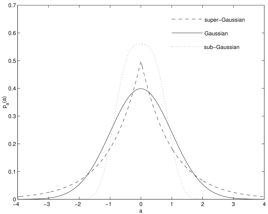
Figure 4: Examples of a sub-Gaussian, a super-Gaussian, and a Gaussian pdf.

Whether a pdf is sub-Gaussian, Gaussian, or super-Gaussian, is commonly seen in the sign of its 4th-order cumulant, $c_{4}.$ It will be respectively, negative, zero, and positive. Data in digital communications are usually sub-Gaussian. Examples of super-Gaussian sources are found in speech and image, among others. The Infomax algorithm of [10] using the logistic nonlinearity was seen to be successful in separating super-Gaussian sources. Instead, it failed for sub-Gaussian mixtures. This is because the nonlinearity $\mbox{\boldmath$g$}(\cdot)$ that was used did not match sufficiently well the sub-Gaussian cdf so that the requirements for stability be met. A simple choice for the score functions corresponding to sub-Gaussian sources is based on the cubic nonlinearity, e.g., $f_{i}(y_{i})=y_{i}^{3}.$ With this choice, $-\kappa_{i}$ is reduced to $c_{4}(y_{i})$. The stability follows since $-\kappa_{i}<0$ is sufficient for (71).

However, when no information on the source statistics is available or the sources are mixed sub- and super-Gaussian, such simple choices are inadequate. Even if one knows which sources are sub- and which are super-Gaussian, there is the problem of unavoidable permutation in the separation result, hence one cannot be sure of which source a function will correspond to. A common approach to overcoming this problem is to parameterize the nonlinearities so as to encompass the expected source distributions. The relevant parameters are then adapted at the same time with the separating matrix [44, 43, 4, 82, 122]. Such could be simply the sign of the estimated $c_{4}(y_{i})$ [82] or, in more sophisticated schemes, a parameter connected with the satisfaction of the stability conditions [103, 122]. A related approach is that of approximating the unknown pdf via a truncated expansion, yielding a polynomial form whose coefficients are determined by the source cumulants [30]. In Section 5.3.1 we discussed a similar approach to the simplification of IT criteria.

Ways of stabilizing an algorithm, that weaken the constraints on the choice of $\mbox{\boldmath$f$}(\cdot)$, have also been developed. The multiplication by the inverse of the Hessian matrix (which is diagonal when using the natural gradient) is shown in [3] to result in a stabilized version. In [94], it is shown that a simple substitution of the term $\mbox{\boldmath$f$}(\mbox{\boldmath$y$}(k))\mbox{\boldmath$y$}^{T}(k)$ in (57) by its transpose, $\mbox{\boldmath$y$}(k)\mbox{\boldmath$f$}(\mbox{\boldmath$y$}^{T}(k))$, suffices to correct an instability in the case that all $f_{i}$ coincide.

7 FastICA and Its Variants

As already mentioned, the source estimates in algorithms based on polynomial nonlinearities $f_{i}$ are not robust to outliers. The criterion (47), involving 4th-order standardized cumulants is an example of this [97]. To address this problem, the following generalized criterion was proposed [103]:

$$\max_{G^{T}G=I}\left(\psi_{F}(\mbox{\boldmath$G$})\stackrel{{\scriptstyle\triangle}}{{=}}\|E[\mbox{\boldmath$F$}(\mbox{\boldmath$y$})-\mbox{\boldmath$F$}(\mbox{\boldmath$y$}^{G})]\|^{2}\right)$$ (73)

where $\mbox{\boldmath$y$}=\mbox{\boldmath$G$}\mbox{\boldmath$u$}$ as before, $\mbox{\boldmath$F$}(\cdot)$ is a smooth, nonlinear, non-quadratic vector function with equal components, $F$, and data prewhitening is assumed, i.e., $G$ is orthogonal. Recall that $\mbox{\boldmath$y$}^{G}$ denotes a Gaussian random vector with the same mean and covariance as $\mbox{\boldmath$y$}.$ In this case, $\mbox{\boldmath$y$}^{G}$ is standardized, i.e., $E[\mbox{\boldmath$y$}^{G}(\mbox{\boldmath$y$}^{G})^{T}]=\mbox{\boldmath$I$}.$ Note that, as in IT criteria discussed above, the underlying principle here is again that of maximizing the distance of the output $y$ from a Gaussian signal, using the nonlinear function $\mbox{\boldmath$F$}(\cdot)$ to extract its HOS.

Let $\mbox{\boldmath$g$}_{i}^{T}$ denote the $i$th row of $\mbox{\boldmath$G$}.$ Then (73) may be equivalently written as:

$$\max_{g_{1},\ldots,g_{N}} \sum_{i=1}^{N}\psi_{F}(\mbox{\boldmath$g$}_{i})$$

subject to $$\mbox{\boldmath$g$}_{i}^{T}\mbox{\boldmath$g$}_{j}=\delta_{ij}$$ (74)

where

$$\psi_{F}(\mbox{\boldmath$g$}_{i})\stackrel{{\scriptstyle\triangle}}{{=}}\left\{E[F(\mbox{\boldmath$g$}_{i}^{T}\mbox{\boldmath$u$})-F(y^{G}_{i})]\right\}^{2}$$ (75)

and $\delta_{ij}$ is the Kronecker delta. Since the second term in (75) is constant, it is at the extrema of $E[F(y_{i})]$ that correspond the maxima of $\psi_{F}(\mbox{\boldmath$g$}_{i}).$ Whether it will be to a maximum or a minimum of $E[F(y_{i})$ depends, respectively, on whether $E[F(y_{i})$ is greater or smaller than $E[F(y_{i}^{G})]$. For $F(y)=y^{4}$ this translates into $y_{i}$ being super- or sub-Gaussian, respectively. For a general $F$, these relations imply generalized definitions of super- and sub-Gaussianity [151].

It is easier to present the optimization of the above criterion by focusing on the extraction of a single source. Once a $\mbox{\boldmath$g$}_{i}$ has been determined, the rest of them can be computed with the additional constraint that they be orthogonal to that already found. This can be repeated for another $\mbox{\boldmath$g$}_{j}$, and so on. Through this so-called deflation approach [69], a single row of $G$ is computed at each step, reducing the problem size by one. Popular methods for enforcing the constraint (74) all along this process include Gram-Schmidt-like orthogonalization schemes [97, 142]. Extracting the sources one by one may be useful not only in view of the simplification this implies for the algorithm, but also in applications that ask for the extraction of only a few of the sources and in a desired order [41]. Furthermore, such an approach may be the only possible solution in cases where not all sources can be recovered at once, for example when $H$ is not invertible (see Section 9).

Consider then the problem of maximizing one of the terms in the sum (74) subject to the constraint that the separating vector $g$ be of unit norm. Assume moreover that $E[F(y)]$ is to be maximized. Then the optimization problem reduces to

$$\max_{\|g\|=1}E[F(\mbox{\boldmath$g$}^{T}\mbox{\boldmath$u$})]$$ (76)

with the following characterization of its stationary points [97]:

$$E[\mbox{\boldmath$u$}f(\mbox{\boldmath$g$}^{T}\mbox{\boldmath$u$})]-\beta\mbox{\boldmath$g$}=\mbox{\boldmath$0$}.$$ (77)

$f$ is the derivative of $F$ and the Lagrange multiplier $\beta$ is given by $\beta=E[yf(y)]$. A steepest ascent scheme yields the update equation:

$$\mbox{\boldmath$g$}(k+1)=\mbox{\boldmath$g$}(k)+\mu(k)\left\{E[\mbox{\boldmath$u$}f(\mbox{\boldmath$g$}^{T}(k)\mbox{\boldmath$u$}]-\beta(k)\mbox{\boldmath$g$}(k)\right\}.$$ (78)

Via a Newton approximation of the above, the following algorithm results [97]:

$$\mbox{\boldmath$g$}^{+}(k+1) = E[\mbox{\boldmath$u$}f(\mbox{\boldmath$g$}^{T}(k)\mbox{\boldmath$u$})]-E[f^{\prime}(\mbox{\boldmath$g$}^{T}(k)\mbox{\boldmath$u$})]\mbox{\boldmath$g$}(k)$$ (79)

$$\mbox{\boldmath$g$}(k+1) = \frac{\mbox{\boldmath$g$}^{+}(k+1)}{\|\mbox{\boldmath$g$}^{+}(k+1)\|}$$ (80)

known as FastICA. The normalization in (80) is needed to enforce the unit-norm constraint and stabilize the algorithm. The connection of the FastICA algorithm, in its multi-source version, with the algorithm (57) was studied in [100]. It was shown that it results as a batch version of (57) via a generalization consisting of the use of not necessarily the same step size for all rows of $\mbox{\boldmath$G$}.$

Note that the above algorithm may be viewed as resulting from (78) by choosing the step size as

$$\mu(k)=\frac{1}{\beta(k)-E[f^{\prime}(\mbox{\boldmath$g$}^{T}(k)\mbox{\boldmath$u$})]}.$$ (81)

It is claimed in [97] that this choice yields the fastest convergence. In fact, as recently shown, $\mu$ should instead be chosen as [151]:

$$\mu(k)=\frac{1}{\beta(k)}$$ (82)

resulting in the following, faster variation of (79)–(80):

$$\mbox{\boldmath$g$}^{+}(k+1) = E[\mbox{\boldmath$u$}f(\mbox{\boldmath$g$}^{T}(k)\mbox{\boldmath$u$})]$$ (83)

$$\mbox{\boldmath$g$}(k+1) = \frac{\mbox{\boldmath$g$}^{+}(k+1)}{\|\mbox{\boldmath$g$}^{+}(k+1)\|}.$$ (84)

The latter algorithm can be viewed as a solution approach to eq. (77) via a fixed-point iteration. In fact, for $F(y)=y^{2p}$ and hence $f(y)=2py^{2p-1}$, it is readily seen to reduce to the so-called super-exponential algorithm (SEA), well-known from the blind deconvolution problem [156, 157]. An interpretation of the SEA as a gradient optimization scheme can be found in [126]. It is the fastest known method for maximizing the ratio $\left|\frac{c_{2p}(y)}{(c_{2}(y))^{p}}\right|$, a criterion known as the minimum-entropy or Donoho’s criterion [71, 182, 50, 152]. In practice $p$ is usually set to two. In that case, $c_{2p}(y)=c_{4}(y)=E[y^{4}]-3(E[y^{2}])^{2}$, and for standardized $y$, $c_{4}(y)=E[y^{4}]-3.$ The connection with (76) when $F(y)=y^{4}$ is thus evident. Note also that for this choice of $F$ the criterion (74) reduces to (47).

Donoho’s criterion has been shown to be equivalent to the so-called constant modulus (CM) criterion, which for $p=2$ reads [107, 108]

$$\min_{g}E[(y^{2}-1)^{2}].$$ (85)

The equivalence holds for $g$ of optimized norm in (85) [148]. Applying a stochastic gradient descent to this criterion results in the celebrated Constant Modulus Algorithm (CMA) [84, 174]:

$$\mbox{\boldmath$g$}(k+1)=\mbox{\boldmath$g$}(k)-\mu(y^{2}(k)-1)y(k)\mbox{\boldmath$u$}(k)$$ (86)

which has been and probably will continue to be one of the major subjects of the blind equalization research [107, 108]. It can be derived as a special case of the algorithm (57) with $f(y)=y^{3}$ and hence, as we saw in Section 6.3, it can only be applied to sub-Gaussian sources. Modified versions that can process super-Gaussian sources can be derived with the aid of the equivalence mentioned above, in view of the ability of the SEA to cope with both kinds of inputs [153].

8 Algebraic Approaches

So far we have been concerned with BSS approaches that stem from optimizing a criterion via a gradient recursive scheme. A great number of methods follow instead an algebraic approach to solving the problem. Although, as we will see shortly, they can also be interpreted as criteria-based schemes, it is their point of view and the tools they employ that differentiate them from the methods discussed above.

8.1 Statistical Approaches

What underlies the algebraic schemes employing statistical quantities is the exploitation of the fact that independence of the components of a vector random process is equivalent to all its cross-cumulants being null. This implies that BSS can be achieved by setting the cross-cumulants of $y$ equal to zero and solving the resulting equations for $\mbox{\boldmath$G$}.$ Such methods have been reported in e.g. [117, 183]. They get too complicated however for realistic problem sizes. Therefore, more efficient and less direct methods are required.

The basic quantity in stochastic algebraic approaches is the cumulant tensor [127]. By tensor we mean here a $q$-way array, i.e., one whose elements are addressed via $q$ indices [18, 53]. It is the 4th-order cumulant of the $N$-vector $y$ that is most commonly encountered. It constitutes a 4th-order tensor, $\mbox{\boldmath$\cal C$}_{4,y}$, with dimensions $N\times N\times N\times N$ [127]. The well-known symmetry property of cumulants [117, 128] implies that $({\cal C}_{4,y})_{i,j,k,l}$ does not depend on the order of its indices. Such a tensor is termed super-symmetric [113].

Another property of cumulants that is employed is that of multilinearity [128, 136]. This refers to the way the cumulants of the output of a linear system are related to those of its input. For the mixing system (7) it takes the form:

$${\rm cum}(u_{i},u_{j},u_{k},u_{l})=\sum_{i_{1},i_{2},i_{3},i_{4}}{\rm cum}(a_{i_{1}},a_{i_{2}},a_{i_{3}},a_{i_{4}})H_{i,i_{1}}H_{j,i_{2}}H_{k,i_{3}}H_{l,i_{4}}.$$ (87)

Using the Tucker product notation [89], this may be written in the more compact way:

$$\mbox{\boldmath$\cal C$}_{4,u}=\mbox{\boldmath$H$}\stackrel{{\scriptstyle{\cal C}_{4,a}}}{{\star}}\mbox{\boldmath$H$}\stackrel{{\scriptstyle{\cal C}_{4,a}}}{{\star}}\mbox{\boldmath$H$}\stackrel{{\scriptstyle{\cal C}_{4,a}}}{{\star}}\mbox{\boldmath$H$}$$ (88)

where $\mbox{\boldmath$\cal C$}_{4,a}$ is diagonal because of the independence of the sources. The above decomposition can thus be viewed as a 4th-order eigenvalue decomposition (EVD) of the 4-way array $\mbox{\boldmath$\cal C$}_{4,u}$ [22, 23] and could be used to blindly identify $\mbox{\boldmath$H$}.$ In contrast to its 2nd-order counterpart, eq. (8), (88) does not suffer from nonuniqueness problems in general. This point will be elaborated upon in the next section.

For the demixing model (6) one may analogously write:

$$\mbox{\boldmath$\cal C$}_{4,y}=\mbox{\boldmath$G$}\stackrel{{\scriptstyle{\cal C}_{4,u}}}{{\star}}\mbox{\boldmath$G$}\stackrel{{\scriptstyle{\cal C}_{4,u}}}{{\star}}\mbox{\boldmath$G$}\stackrel{{\scriptstyle{\cal C}_{4,u}}}{{\star}}\mbox{\boldmath$G$}$$ (89)

or, in terms of the global system $\mbox{\boldmath$S$}=\mbox{\boldmath$G$}\mbox{\boldmath$H$}$ [89]:

$$\mbox{\boldmath$\cal C$}_{4,y}=\mbox{\boldmath$S$}\stackrel{{\scriptstyle{\cal C}_{4,a}}}{{\star}}\mbox{\boldmath$S$}\stackrel{{\scriptstyle{\cal C}_{4,a}}}{{\star}}\mbox{\boldmath$S$}\stackrel{{\scriptstyle{\cal C}_{4,a}}}{{\star}}\mbox{\boldmath$S$}.$$ (90)

Assume $u$ has been standardized. It can be shown that an orthogonal $G$ in (89) leaves the norm of $\mbox{\boldmath$\cal C$}_{4,u}$ unchanged:

$$\|\mbox{\boldmath$\cal C$}_{4,y}\|=\|\mbox{\boldmath$\cal C$}_{4,u}\|.$$ (91)

This has very important implications for contrasts of the type given in (47). It follows that maximizing the sum of the autocumulants squared is equivalent to minimizing the sum of the cross-cumulants squared. This brings us back to the cross-cumulant nulling idea discussed above and shows (47) to be a cumulant tensor diagonalization criterion [49, 36].

It has been shown that for $N=2$ sources the above maximization can be given a closed-form solution, since $G$ is then a simple Givens rotation matrix [48]. For $N>2$ a Jacobi-type algorithm [85] was proposed that iteratively processes the components of $y$ in pairs [48]. In addition to being simple and efficient, this method relies on the theoretical result that pairwise independence, under some weak constraints, is sufficient for ICA [48, 20]. The resulting algorithm has been seen to be a batch version of the nonlinear PCA rule presented in Section 6 [83]. Though proven to be effective in practice, no theoretical proof of its global convergence has been devised yet [47]. The same basic idea, of employing iterative Jacobi rotations to effect a diagonalization, can be found in a number of other approaches as well, e.g., [38, 181, 159].

A method for indirectly diagonalizing $\mbox{\boldmath$\cal C$}_{4,u}$, via a joint diagonalization of a set of related matrices was proposed in [38]. It can in fact be shown that a single matrix suffices, provided it is properly chosen [172]. However, since this choice is not easy to make due to the blind nature of the problem, a set of matrices is normally employed. An example could be the set of slices of $\mbox{\boldmath$\cal C$}_{4,u}$ [38]. It turns out however that the eigematrices of $\mbox{\boldmath$\cal C$}_{4,u}$, resulting from the EVD of the corresponding symmetric operator, provide a much smaller sufficient set. This leads to an efficient algorithm, known as Joint Approximate Diagonalization of Eigenmatrices (JADE) [38, 179]. It can be seen to correspond to the optimization of a cost similar to (47), in which only the cross-cumulants having their first and second indices different are minimized. An even weaker criterion, that proves nevertheless to be effective, was proposed in [65].

Another way of obtaining the decomposition (88) is via an extension of the EVD to tensors, called Higher-Order EigenValue Decomposition (HO-EVD) and proposed and studied in [61, 59, 63]. It approximates (88) with the aid of a singular value decomposition (SVD) of $\mbox{\boldmath$\cal C$}_{4,u}$ unfolded to a $N\times N^{3}$ matrix. The so-called core tensor however, approximating $\mbox{\boldmath$\cal C$}_{4,a}$, is not guaranteed to be diagonal, unless of course the given data exactly satisfy the assumed model and the cumulant estimates are exact, which is rarely the case. Hence, this method usually serves to provide a good initialization to some other, iterative algorithm. See [65] for an interpretation of HO-EVD as a cost-optimizing method.

8.2 Deterministic Approaches

The methods described above work with statistical quantities, estimated from the given data. Approaches that act directly on the data also exist and could be referred to as deterministic. The best way of conveying the basic idea is by looking at algebraic methods for solving the CM cost minimization problem. Note that the Kronecker product allows us to write the square of $y=\mbox{\boldmath$g$}^{T}\mbox{\boldmath$u$}$ in the form

$$y^{2}=(\mbox{\boldmath$g$}\otimes\mbox{\boldmath$g$})^{T}(\mbox{\boldmath$u$}\otimes\mbox{\boldmath$u$}).$$ (92)

Let us take a block of observation vectors, say $\mbox{\boldmath$u$}(1),\mbox{\boldmath$u$}(2),\ldots,\mbox{\boldmath$u$}(T)$. Observe that the minimum CM criterion (85) aims at approximating $y^{2}$ by one. In view of (92) this can be stated as the algebraic problem of decomposing the solution, $w$, to the following $T\times N^{2}$ linear system of equations

$$\underbrace{\left[\begin{array}[]{c}(\mbox{\boldmath$u$}(1)\otimes\mbox{\boldmath$u$}(1))^{T}\\ (\mbox{\boldmath$u$}(2)\otimes\mbox{\boldmath$u$}(2))^{T}\\ \vdots\\ (\mbox{\boldmath$u$}(T)\otimes\mbox{\boldmath$u$}(T))^{T}\end{array}\right]}_{\mbox{\boldmath$P$}}\mbox{\boldmath$w$}=\underbrace{\left[\begin{array}[]{c}1\\ 1\\ \vdots\\ 1\end{array}\right]}_{\mbox{\boldmath$1$}}$$ (93)

in the Kronecker square form $\mbox{\boldmath$w$}=\mbox{\boldmath$g$}\otimes\mbox{\boldmath$g$}$ [181, 87, 88].

Note that (93) is not square and for $T>N^{2}$ (common assumption) is overdetermined. A solution $w$ is not in general decomposable as above. [87, 88] consider solving (93) in the LS sense and then approximating the result by a Kronecker square to yield the separation filter. A more sophisticated approach is followed by the Analytical Constant Modulus Algorithm (ACMA) [181, 180] and applied to the multi-source extraction problem. A basis, $\{\mbox{\boldmath$w$}_{1},\mbox{\boldmath$w$}_{2},\ldots,\mbox{\boldmath$w$}_{N}\}$, for the solution set of (93) is first computed and then approximated by another whose vectors have the form $\mbox{\boldmath$g$}\otimes\mbox{\boldmath$g$}.$ This approximation is seen to lead again to a joint diagonalization problem, involving the matrices $\mbox{\boldmath$W$}_{i}={\rm unvec}(\mbox{\boldmath$w$}_{i}).$

Deterministic approaches have the advantage of requiring only a few data to provide a good estimate for $G$ [181]. Interestingly, the ACMA solution was shown to asymptotically converge to the CM one, when $T\rightarrow\infty$ [180].

9 Undermodeling: Problems and Solutions

We have thus far assumed that $H$ is square, or as it is otherwise said, that there as many sensors as sources. A more realistic scenario would involve a rectangular mixing matrix, of dimensions $M\times N$ with $M$ not necessarily equal to $N$. In this section we will be concerned with the problems that emerge in such a case and possible approaches to their solution.

First, let us consider the case of more sensors than sources, with a full column rank mixing matrix. This is the case studied in the majority of the BSS works as it presents no particular difficulties compared to that of square $\mbox{\boldmath$H$}.$ The reason for this, as already explained in Section 2, is that an $H$ with more rows than columns can be easily inverted, provided of course that it be of full column rank. Moreover, this case reduces to the simpler one as a result of a sphereing operation. Indeed, if $H$ is $M\times N$ with $M>N$ in (8), an EVD of $\mbox{\boldmath$R$}_{u}$ will yield an orthonormal basis for its range, represented by a columnwise orthogonal matrix $A$, revealing at the same time the number of sources, $N$. Therefore, there will be an $N\times N$ orthogonal matrix $\mbox{\boldmath$Q$}^{T}$ such that $\mbox{\boldmath$A$}=\mbox{\boldmath$H$}\mbox{\boldmath$Q$}^{T}.$ Transforming the mixture data as $\mbox{\boldmath$\bar{u}$}(n)=\mbox{\boldmath$A$}^{T}\mbox{\boldmath$u$}(n)$ will then result in the $N$-source, $N$-sensor system $\mbox{\boldmath$\bar{u}$}(n)=\mbox{\boldmath$Q$}\mbox{\boldmath$a$}(n)$ with an orthogonal mixing matrix. From this point on, a method for square systems can be applied.

The case of less sensors than sources is however much more difficult to be studied. Recall from Section 2 that this includes the existence of noise sources as a special case. A consequence of the noninvertibility of $H$ is that, in contrast to the case of $M\geq N$, the mixing system identification and source extraction are two different problems. Even if $H$ is perfectly known, it is not clear how it could be inverted to recover $\mbox{\boldmath$a$}.$ It was recently proved [167] that $H$ is uniquely determined if there are no Gaussian sources. Furthermore, the source vector can be extracted only up to an unknown additive noise vector [167].

9.1 Identification

If $M<N$, $H$ cannot have linearly independent columns. It can however be that the projectors on these columns be linearly independent. This means that the $M^{2}\times N$ matrix $\mbox{\boldmath$H$}\odot\mbox{\boldmath$H$}$, where $\odot$ denotes the Kronecker columnwise product [161], can be of full column rank if $M^{2}>N.$ Based on this assumption, [24] develops an algebraic algorithm for identifying $\mbox{\boldmath$H$}.$ The decomposition of $\mbox{\boldmath$\cal C$}_{4,u}$ in its eigenmatrices mentioned above is a basic step in this algorithm. In fact, the method of [24] reduces to that for the case of $M\geq N.$ The maximum number of sources the algorithm can afford to can be shown to be of the order of $M^{2}$ [24].

The result is the decomposition of the tensor $\mbox{\boldmath$\cal C$}_{4,u}$ in a sum of $N$ linearly independent rank-1 tensors, that is 4th-order outer products, as in:

$$\mbox{\boldmath$\cal C$}_{4,u}=c_{4}(a_{1})\mbox{\boldmath$h$}_{1}\star\mbox{\boldmath$h$}_{1}\star\mbox{\boldmath$h$}_{1}\star\mbox{\boldmath$h$}_{1}+c_{4}(a_{2})\mbox{\boldmath$h$}_{2}\star\mbox{\boldmath$h$}_{2}\star\mbox{\boldmath$h$}_{2}\star\mbox{\boldmath$h$}_{2}+\cdots+c_{4}(a_{N})\mbox{\boldmath$h$}_{N}\star\mbox{\boldmath$h$}_{N}\star\mbox{\boldmath$h$}_{N}\star\mbox{\boldmath$h$}_{N}$$ (94)

where $\mbox{\boldmath$h$}_{j}$ is the $j$th column of $H$ and

$$\left(\mbox{\boldmath$h$}_{j}\star\mbox{\boldmath$h$}_{j}\star\mbox{\boldmath$h$}_{j}\star\mbox{\boldmath$h$}_{j}\right)_{i_{1},i_{2},i_{3},i_{4}}\stackrel{{\scriptstyle\triangle}}{{=}}H_{i_{1},j}H_{i_{2},j}H_{i_{3},j}H_{i_{4},j}.$$

We say that this tensor has rank $N$ since it cannot be decomposed in less than $N$ such terms. Eq. (94) is an instance of a decomposition model for general, not necessarily super-symmetric tensors, known in multi-way data analysis with the name Parallel Factor Analysis (PARAFAC) [16] (or CANonical DECOMPosition (CANDECOMP) [59]). For a 4th-order $M_{1}\times M_{2}\times M_{3}\times M_{4}$ tensor $\cal A$ it takes the form:

$$\mbox{\boldmath$\cal A$}=\mbox{\boldmath$U$}^{(1)}\stackrel{{\scriptstyle\cal S}}{{\star}}\mbox{\boldmath$U$}^{(2)}\stackrel{{\scriptstyle\cal S}}{{\star}}\mbox{\boldmath$U$}^{(3)}\stackrel{{\scriptstyle\cal S}}{{\star}}\mbox{\boldmath$U$}^{(4)}$$ (95)

where $\mbox{\boldmath$U$}^{(i)}$ is an $M_{i}\times r$ matrix, $r={\rm rank}(\mbox{\boldmath$\cal A$})$ and $\cal S$ is an $r\times r\times r\times r$ diagonal tensor. The PARAFAC of a 3rd-order tensor is schematically shown in Fig. 5.

Figure 5: PARAFAC analysis of a 3rd-order tensor.

PARAFAC extends to higher-order tensors the well-known expansion of a matrix $A$ in a sum of ${\rm rank}(\mbox{\boldmath$A$})$ rank-1 terms [85]. In contrast to what holds in second-order tensors however, this decomposition enjoys the property of uniqueness under some rather weak conditions. This fact, along with the possibility of interpreting the BSS problem as one of determining the independent factors generating the observed data [78], led to a recent research activity for applying it to blind signal processing problems [161]. A sufficient but not necessary condition for uniqueness of the factors has been first derived in [114] for 3rd-order tensors and recently extended to arrays of higher orders [160]. For the tensor in (94) this condition leads, generically, to

$$4M\geq 2N+3.$$ (96)

This means that the uniqueness will be ensured for roughly up to $2M$ sources. This should be compared with the $M^{2}$ sources that are possible in the method of [24]. Note however that the condition of [160] applies to general tensors, not only to cumulants of linear mixtures.

For a tensor that exactly satisfies a PARAFAC of rank $N$, methods based on joint diagonalization of matrices have been derived; see, e.g., [59]. Nonetheless, exact decomposition may not be possible in practice and it will have to be approximated. Alternating Least Squares (ALS) provide the most common algorithm for this task, referred to sometimes as the PARAFAC ALS algorithm [16, 17]. The idea is to alternately optimize the matrix $\mbox{\boldmath$U$}^{(i)}$ in every dimension, in the LS sense, considering the other matrices fixed. For a super-symmetric tensor, such as that given in (95), the same method applies without imposing the equality of these matrices. The final approximation however turns out to be symmetric. This procedure is provenly convergent, though not necessarily to a good solution. For super-symmetric tensors, HO-EVD yields an initialization which has been observed to be effective in leading to good approximations [59].

An approach to computing the PARAFAC of a super-symmetric tensor that respects the symmetry property and relies on the correspondence between super-symmetric tensors and homogeneous multivariate polynomials was proposed in [57]. It is shown that, in this new domain, the PARAFAC problem translates into writing a polynomial as a sum of powers of linear forms [57]. Despite the sound theoretical foundations of this approach however, working algorithms could only be developed for small-sized problems [57, 51, 62].

9.2 Inversion

As already explained, no linear inversion is possible in general for a system with more sources than sensors. Nevertheless, it was proved in [167] that inversion is possible in case that the sources take values from a finite set. [51] presents an algorithm for nonlinearly inverting an identified mixing system with discrete inputs. The basic idea is that discreteness of signals with alphabets as those used in digital communications can be expressed in terms of polynomial equations. Writing appropriate polynomial equations for the $u_{i}$’s in terms of $H$ and the $a_{i}$’s and using the equations characterizing the discrete range of the latter, a nonlinear system of equations in the $a_{i}$’s results. Hopefully, this will not contain many nonlinear combinations of the sources. These are considered as additional unknowns so the system becomes linear and can be solved with a LS method. The ‘nonlinear’ unknowns are then discarded from the solution.

An alternative way out is to follow a deflation approach, extracting the sources one by one [20]. Note that this problem can be viewed as a particular case of the PARAFAC decomposition of $\mbox{\boldmath$\cal C$}_{4,u}$ where only a rank-1 term is computed at a time. For the tensor $\mbox{\boldmath$\cal C$}_{4,u}$ this yields the Donoho’s criterion [112]. The ALS algorithm described above reduces to a higher-order extension of the well-known power method for rank-1 matrix approximation [85], known as higher-order power method (HO-PM) [60, 64]. A version of the HO-PM, adapted to super-symmetric tensors, was recently introduced [112, 113]. Interestingly, the SEA of [153] turns out to be nothing but this method applied to the tensor $\mbox{\boldmath$\cal C$}_{4,u}$ [112].

Donoho’s cost functional,

$$\psi_{D}(\mbox{\boldmath$g$})\stackrel{{\scriptstyle\triangle}}{{=}}\left|\frac{c_{4}(y)}{[c_{2}(y)]^{2}}\right|,\mbox{\ \ }y=\mbox{\boldmath$g$}^{T}\mbox{\boldmath$u$}$$ (97)

is multimodal. Most importantly, its local extrema might correspond to separating filters of a very low performance compared to the globally optimal ones. This issue has been extensively studied, especially in the context of CM equalization [107, 108]. To deal with this problem, one would like to have a good initial estimate for $g$ that would lie in the basin of attraction of a globally optimal solution. This would lead the gradient algorithm to a separator of acceptable performance. Such an initialization scheme was devised in [149] and consists of two successive matrix rank-1 approximations (data prewhitening is assumed) :

1. First build from $\mbox{\boldmath$\cal C$}_{4,u}$ the $M^{2}\times M^{2}$ symmetric matrix $\mbox{\boldmath$C$}_{u}$ by combining the first two dimensions in the row dimension and the other two in the column dimension.

2. Compute the best in the LS sense rank-1 approximation of $\mbox{\boldmath$C$}_{u}$:

   $$\hat{\mbox{\boldmath$C$}}_{u}=\lambda\mbox{\boldmath$w$}\mbox{\boldmath$w$}^{T}.$$

3. Compute the best in the LS sense rank-1 approximation of the $M\times M$ symmetric matrix $\mbox{\boldmath$W$}={\rm unvec}(\mbox{\boldmath$w$})$:

   $$\hat{\mbox{\boldmath$W$}}=\varsigma\mbox{\boldmath$g$}^{0}(\mbox{\boldmath$g$}^{0})^{T}$$

4. Initialize the SEA with $\mbox{\boldmath$g$}^{0}.$

Note the similarity with the deterministic approaches discussed in Section 8.2. This method has been seen via extensive simulations to frequently outperform the HO-EVD initialization scheme in terms of the proximity of the estimate provided to the globally optimal solution. Fig. 6 depicts the initial estimates computed with these two methods and the corresponding trajectories followed by the SEA, for a 3-sensor, 7-source system with mixed sub- and super-Gaussian sources.

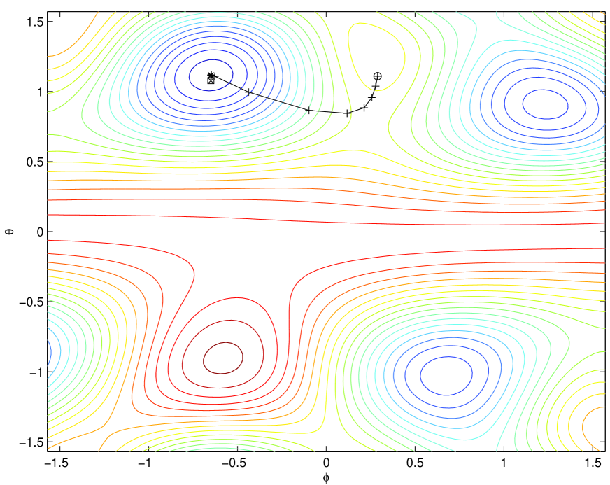
Figure 6: Visualization of the SEA for two initialization methods. The HO-EVD-based estimate is denoted by a small circle and the trajectory followed by $+$’s. The initial estimate provided by the method of [149] is denoted by a small square and the subsequent estimates by $\times$’s. The angles $\theta$ and $\phi$ parameterize the unit-norm 3-vector $\mbox{\boldmath$g$}(k).$

As shown in the figure, the initialization $\mbox{\boldmath$g$}^{0}$ computed with the above method lies so close to the global optimum that SEA iterations are hardly needed. In fact, it can be shown [150] that $\mbox{\boldmath$g$}^{0}$ will equal a perfect separator if it exists (that is, when $M\geq N$). More generally and for sources that are all sub- or super-Gaussian, the resulting separation performance is shown to be bounded as [149]:

$$\varsigma^{2}|\lambda|\leq\psi_{D}(\mbox{\boldmath$g$}^{0})\leq|\lambda|.$$ (98)

Notice that these bounds are computable a-priori, that is, based on only the observation data statistics.

In view of the above discussion, it can be seen that an approximation to the Donoho’s criterion, given as:

$$\max_{\|g\|=1}\left(\hat{\psi}_{D}(\mbox{\boldmath$g$})\stackrel{{\scriptstyle\triangle}}{{=}}\left|\lambda(\mbox{\boldmath$g$}^{T}\mbox{\boldmath$W$}\mbox{\boldmath$g$})^{2}\right|\right),$$ (99)

could be an interesting alternative. First, this cost is readily verified to be unimodal, in the sense that all its stable stationary points correspond to separators of the same quality. Next, it inherits all the good properties of the initialization given above. An algorithm based on this criterion would be globally convergent, that is, its convergent points would be independent of its initialization. Moreover, they would provide high performance separating filters. Such an algorithm was developed and successfully tested in [150] and is described by the following two recursions:

$$\mbox{\boldmath$W$}(k+1) = \mbox{\boldmath$W$}(k)+\frac{\mu_{1}}{1+\mu_{1}\|\mbox{\boldmath$u$}(k)\otimes\mbox{\boldmath$u$}(k)\|^{2}}\left(1-\mbox{\boldmath$u$}^{T}(k)\mbox{\boldmath$W$}(k)\mbox{\boldmath$u$}(k)\right)\mbox{\boldmath$u$}(k)\mbox{\boldmath$u$}^{T}(k)$$ (100)

$$\mbox{\boldmath$g$}^{+}(k+1) = \mbox{\boldmath$g$}(k)+\mu_{2}\mbox{\boldmath$W$}(k+1)\mbox{\boldmath$g$}(k)$$ (101)

$$\mbox{\boldmath$g$}(k+1) = \frac{\mbox{\boldmath$g$}^{+}(k+1)}{\|\mbox{\boldmath$g$}^{+}(k+1)\|}.$$ (102)

Fig. 7 shows the output of a length-80 equalizer $\mbox{\boldmath$g$}(k)$ for a 2-source, 4-sensor dynamic mixing system of order 29, with binary (+1,-1), i.i.d. inputs.

Figure 7: Output of the equalizer, adapted with (100), (101), (102).

10 Extensions

The BSS problem studied in the last example concerns a dynamic system with 4 sensors and 2 sources. Its transfer function can be written as:

$$\mbox{\boldmath$H$}(z)=\mbox{\boldmath$H$}_{0}+\mbox{\boldmath$H$}_{1}z^{-1}+\cdots+\mbox{\boldmath$H$}_{29}z^{-29}$$ (103)

where the $4\times 2$ matrices $\mbox{\boldmath$H$}_{i}$ are the coefficients of its impulse response. The deconvolution filter is given in the $\cal Z$-domain by the $4\times 1$ transfer function

$$\mbox{\boldmath$g$}(z)=\mbox{\boldmath$g$}_{0}+\mbox{\boldmath$g$}_{1}z^{-1}+\cdots+\mbox{\boldmath$g$}_{19}z^{-19}$$ (104)

with the $\mbox{\boldmath$g$}_{i}$’s being $4\times 1$ vectors. The separating vector $g$ adapted with the above algorithm is built from $\mbox{\boldmath$g$}(z)$ as:

$$\mbox{\boldmath$g$}=\left[\begin{array}[]{cccc}\mbox{\boldmath$g$}_{0}^{T}&\mbox{\boldmath$g$}_{1}^{T}&\cdots&\mbox{\boldmath$g$}_{19}^{T}\end{array}\right]^{T}$$ (105)

and has dimensions $80\times 1.$ This problem can be re-expressed in the form $\mbox{\boldmath$u$}=\mbox{\boldmath$H$}\mbox{\boldmath$a$}$ where the matrix $H$ has the special structure:

$$\mbox{\boldmath$H$}=\left[\begin{array}[]{cccccc}\mbox{\boldmath$H$}_{0}&\mbox{\boldmath$H$}_{1}&\cdots&\mbox{\boldmath$H$}_{29}&\cdots&\bigcirc\\ &\mbox{\boldmath$H$}_{0}&\cdots&\mbox{\boldmath$H$}_{28}&\mbox{\boldmath$H$}_{29}&\\ \vdots&\ddots&\ddots&\ddots&\ddots&\vdots\\ \bigcirc&\cdots&\mbox{\boldmath$H$}_{0}&\cdots&\cdots&\mbox{\boldmath$H$}_{29}\end{array}\right]$$ (106)

and dimensions $80\times 98$.

This example shows that the model (7) can also describe convolutive mixtures provided an appropriate structure is imposed on $\mbox{\boldmath$H$}.$ The relations between the BSS and blind deconvolution problems are discussed in [75]. That work also considers deriving BSS algorithms like that of (57) that take into account the rich structure present in $\mbox{\boldmath$H$}.$ Similar adaptive algorithms for blind equalization are derived in [184]. In that context, equivariance translates into robustness to channel ill-conditioning [184]. The definition of the natural gradient has been extended to dynamic matrices as well, giving rise to efficient and fast algorithms [4]. Contrast functions for convolutive mixture separation were derived in [50] and later generalized in [132]. Classical multichannel blind deconvolution HOS-based algorithms [178] also find application here. One of the few such works known to cope with the underdetermined case is presented in [170]. For more works on convolutive mixture separation, see, e.g., [5, 40, 41, 68, 73, 77, 118, 120, 162, 173, 176, 177, 189].

Although, as we saw, the noisy case can be studied in the context of undermodeled systems, a great number of works, dealing explicitly with noisy mixtures, have also been reported; see, e.g., [46, 74, 98, 133].

There are applications that involve independent source mixing via a nonlinear system. These include satellite channels, magnetic recording channels, etc [169]. The type of the nonlinearity suggests the possible separation approaches. In [186] a multilayer perceptron is used as a separator. Post-nonlinear mixtures, that is, instantaneous linear mixing systems followed by entrywise zero-memory nonlinearites, are studied in [167]. In both of these works IT criteria as those discussed here and related algorithms are employed. Self-organizing maps are proposed in [140]. A more recent work [169] concerns post-nonlinear convolutive systems.

The case of nonstationary sources has also been recently addressed; see, e.g., [39, 42, 110, 145]. Time-varying mixing systems with stationary sources are studied in [144] where it is shown that for slow variations a solution is possible by making use of techniques derived for time-invariant mixtures.

11 Concluding Remarks

We gave an overview of the various forms of the BSS problem and approaches to its solution. Classical and well-established as well as more recent approaches were discussed in a unifying framework, putting an emphasis on their connections.

It has to be noted that not all existing BSS works could be included in such a short course. Only a representative sample was presented, hopefully sufficiently motivating for further study. Material left out includes, for example, works on state-space approaches to BSS (e.g., [188]), EM-based algorithms (e.g., [13]), sparse coding and feature extraction (e.g., [105]), independent analysis of subspace components [31, 67], etc.

The interested readers may consult the relevant (immense) bibliography. In our list of references, tutorial and review material is marked in boldface. WWW sites devoted to BSS, with tutorials, research papers, software and demos, have also been built and their number is still increasing. A good starting point is http://www.media.mit.edu/ paris/ica.html.

BSS is a topic that can be considered to have reached a certain maturity, in both its theory and algorithmic schemes. Yet unanswered questions concerning mainly the understanding of the behavior and implementation issues of BSS algorithms still exist. Moreover, new application fields are being discovered and connections with seemingly unrelated disciplines are brought out, opening new, promising research directions. One would thus be justified to feel that BSS will continue to be a research subject of high interest for the years to come.

References

- [1] U. R. Abeyratne, A. P. Petropulu, and J. M. Reid, “Higher-order spectra based deconvolution of ultrasound images,” IEEE Trans. Ultrasonics, Ferroelectrics, and Frequency Control, vol. 42, no. 6, pp. 1064–1095, Nov. 1995.
- [2] S. Amari, “Natural gradient works efficiently in learning,” Neural Computation, vol. 10, pp. 251–276, 1998.
- [3] S. Amari, T.-P. Chen, and A. Cichocki, “Stability analysis of adaptive blind source separation,” Neural Networks, vol. 10, no. 8, pp. 1345–1351, 1997.
- [4] S. Amari and A. Cichocki, “Adaptive blind signal processing – Neural network approaches,” pp. 2026–2048 in [164].
- [5] S. Amari, S. C. Douglas, A. Cichocki, and H. H. Yang, “Multichannel blind deconvolution and equalization using the natural gradient,” Proc. IEEE Int’l Symp. Wireless Communications, pp. 101-107, 1997.
- [6] B. Arons, “A review of the cocktail party effect,” Journal of the American Voice I/O Society, vol. 12, pp. 35–50, Jul. 1992.
- [7] A. K. Barros, A. Mansour, and N. Ohnishi, “Removing artifacts from electrocardiographic signals using independent components analysis,” Neurocomputing, vol. 22, no. 1–3, pp. 173–186, Nov. 1998.
- [8] R. H. T. Bates, “Astronomical speckle imaging,” Physics Reports, vol. 90, no. 4, pp. 203–297, 1982.
- [9] A. J. Bell, “Information theory, independent-component analysis, and applications,” pp. 237–264 in [92].
- [10] A. J. Bell and T. J. Sejnowski, “An information-maximization approach to blnd separation and blind deconvolution,” Neural Computation, vol. 7, pp. 1129–1159, 1995.
- [11] ——, “Edges are the ‘independent components’ of natural scenes,” Advances in Neural Information Processing Systems 9 (NIPS-96), 1996.
- [12] S. Bellini, “Bussgang techniques for blind deconvolution and equalization,” pp. 8–59 in [90].
- [13] A. Belouchrani and J.-F. Cardoso, “Maximum likelihood source separation by the expectation-maximization technique: Deterministic and stochastic implementation,” Proc. NOLTA-95, pp. 49–53.
- [14] A. Benveniste, M. Goursat, and G. Ruget, “Robust identification of a nonminimum phase system: Blind adjustment of a linear equalizer in data communications,” IEEE Trans. Automatic Control, vol. 25, no. 3, pp. 385–399, June 1980.
- [15] J. J. Bussgang, “Crosscorrelation functions of amplitude-distorted Gaussian signals,” Technical Report 216, MIT Res, Lab. Electronics, pp. 1–14, March 1952.
- [16] R. Bro, “PARAFAC: Tutorial and applications,” Chemometrics and Intelligent Laboratory Systems, vol. 38, pp. 149–171, 1997.
- [17] R. Bro, N. Sidiropoulos, and G. B. Giannakis, “A fast least squares algorithm for separating trilinear mixtures,” Proc. ICA-99, pp. 289–294.
- [18] D. S. Burdick, “An introduction to tensor products with applications to multiway data analysis,” Chemometrics and Intelligent Laboratory Systems, vol. 28, pp. 229–237, 1995.
- [19] J. A. Cadzow, “Blind deconvolution via cumulant extrema,” IEEE Signal Processing Magazine, pp. 24–42, May 1996.
- [20] X. Cao and R. Liu, “General approach to blind source separation,” IEEE Trans. Signal Processing, vol. 44, no. 3, pp. 562–571, March 1996.
- [21] J.-F. Cardoso, “Source separation using higher order moments,” Proc. ICASSP-89, pp. 2109–2112.
- [22] ——, “Localisation et identification par la quadricovariance,” Traitement du Signal, vol. 7, no. 5, pp. 397–406, Dec. 1990.
- [23] ——, “Eigen-structure of the fourth-order cumulant tensor with application to the blind source separation problem,” Proc. ICASSP-90, pp. 2655–2658.
- [24] ——, “Super-symmetric decomposition of the fourth-order cumulant tensor. Blind identification of more sources than sensors,” Proc. ICASSP-91, pp. 3109–3112.
- [25] ——, “Higher-order narrow-band array processing,” Proc. Int’l Sig. Proc. Wkshp on Higher-Order Statistics, 1991.
- [26] ——, “On the performance of orthogonal source separation algorithms,” Proc. EUSIPCO-94.
- [27] ——, “A tetradic decomposition of 4th-order tensors: application to the source separation problem,” pp. 375–382 in [131].
- [28] ——, “Quelques principes de séparation de sources,” in École des techniques avancées signal-image-parole, 1996.
- [29] ——, “Infomax and maximum likelihood for blind source separation,” IEEE Signal Processing Letters, vol. 4, no. 4, pp. 112–114, April 1997.
- [30] ——, “Blind signal separation: statistical principles,” Proc. IEEE, vol. 86, no. 10, pp. 2009–2025, Oct. 1998.
- [31] ——, “Multidimensional independent component analysis,” Proc. ICASSP-98, pp. 1941–1944.
- [32] ——, “Learning in manifolds: The case of source separation,” Proc. SSAP-98, pp. 136–139.
- [33] ——, “High-order contrasts for independent component analysis,” Neural Computation, vol. 11, no. 1, pp. 157–192, Jan. 1999.
- [34] ——, “Entropic contrasts for source separation: Geometry and stability,” pp. 139–189 in [92].
- [35] ——, Lecture in GdR Meeting on Blind Source Separation, École Nationale Supérieure des Télécommunications (ENST), Paris, 2000.
- [36] J.-F. Cardoso and P. Comon, “Independent component analysis: A survey of some algebraic methods,” Proc. ISCAS-96, pp. 93–96.
- [37] J.-F. Cardoso and B. H. Laheld, “Equivariant adaptive source separation,” IEEE Trans. Signal Processing, vol. 44, no. 12, pp. 3017–3030, Dec. 1996.
- [38] J.-F. Cardoso and A. Souloumiac, “Blind beamforming for non-Gaussian signals,” Proc. IEE, Part F, vol. 140, no. 6, pp. 362–370, Dec 1993.
- [39] C. Chang, Z. Ding, S.-F. Yau, and F. H. Y. Chan, “Matrix-pencil approach to blind separation of colored nonstationary signals,” IEEE Trans. Signal Processing, vol. 48, no. 3, pp. 900–907, March 2000.
- [40] B. Chen, A. Petropulu, L. De Lathauwer, and B. De Moor, “Blind MIMO system identification based on cross-polyspectra,” Proc. EUSIPCO-2000.
- [41] S. Choi and A. Cichocki, “Cascade neural networks for multichannel blind deconvolution,” Electronics Letters, vol. 34, no. 12, pp. 1186–1187, June 1998.
- [42] ——, “Blind separation of nonstationary sources in noisy mixtures,” ELectronics Letters, vol. 36, no. 9, pp. 848–849, 2000.
- [43] A. Cichocki, J. Karhunen, W. Kasprzak, and R. Vigário, “Neural networks for blind separation with unknown number of sources,” Neurocomputing, vol. 24, pp. 55–93, 1999.
- [44] A. Cichocki, I. Sabala, S. Choi, B. Orsier, and R. Szupiluk, “Self-adaptive independent component analysis for sub-Gaussian and super-Gaussian mixtures with an unknown number of sources and additive noise,” Proc. NOLTA-97, pp. 731–734.
- [45] A. Cichocki, R. Unbehauen and E. Rummert, “Robust learning algorithm for blind separation of signals,” Electronics Letters, vol. 30, no. 17, pp. 1386–1387, Aug. 1994.
- [46] P. Comon, “Analyse en composantes indépendantes et identification aveugle,” Traitement du Signal, vol. 7, no. 3, pp. 435–450, Dec. 1990.
- [47] ——, “Remarques sur la diagonalisation tensorielle par la methode de Jacobi,” Proc. GRETSI-93, pp. 125–128.
- [48] ——, “Independent component analysis, a new concept ?,” Signal Processing, vol. 36, pp. 287–314, April 1994.
- [49] ——, “Tensor diagonalization, a useful tool in signal processing,” Proc. IFAC-SYSID-94, pp. 77–82.
- [50] ——, “Contrasts for multichannel blind deconvolution,” IEEE Signal Processing Letters, vol. 3, no. 7, pp. 209–211, July 1996.
- [51] ——, “Blind channel identification and extraction of more sources than sensors,” keynote address in SPIE Conference, San Diego, July 19-24 1998, pp. 2–13.
- [52] ——, “Block methods for channel identification and source separation,” Proc. IEEE Symp. Adapt. Syst. Sig. Proc. Commun. Control, pp. 87–92, 2000.
- [53] ——, “Tensor decompositions: State of the art and applications,” keynote address in IMA Conf. Mathematics in Signal Processing, Warwick, UK, Dec. 18-20, 2000.
- [54] ——, “From source separation to blind equalization – Contrast-based approaches,” Proc. ICISP-2001, pp. 20–32.
- [55] P. Comon and P. Chevalier, “Source separation: Models, concepts, algorithms and performance,” pp. 191–236 in [92].
- [56] P. Comon, L. De Lathauwer, and B. De Moor, “An algorithm for ICA with 3 sources and 2 sensors,” Proc. Sixth Sig. Proc. Workshop on Higher Order Statistics, Ceasarea, Israel, June 14–16 1999, pp. 116–120.
- [57] P. Comon and B. Mourrain, “Decomposition of quantics in sums of powers of linear forms,” Signal Processing, vol. 53, pp. 93–107, 1996.
- [58] R. Coppi and S. Bolasco (eds.), Multiway Data Analysis, Elsevier North-Holland, 1989.
- [59] L. De Lathauwer, Signal Processing Based on Multilinear Algebra, Ph.D. thesis, K.U.Leuven, Sept. 1997.
- [60] L. De Lathauwer, P. Comon, B. De Moor, and J. Vandewalle, ‘Higher-order power method – Application in independent component analysis,” Proc. NOLTA-95.
- [61] L. De Lathauwer, B. De Moor, and J. Vandewalle, “Blind source separation by higher-order singular value decomposition,” Proc. EUSIPCO-94, pp. 175–178.
- [62] ——, “An algebraic ICA algorithm for 3 sources and 2 sensors,” Proc. EUSIPCO-2000.
- [63] ——, “A multilinear singular value decomposition”, SIAM J. Matrix Anal. Appl., vol. 21, no. 4, pp. 1253–1278, Apr. 2000.
- [64] ——, “On the best rank-1 and rank- approximation and applications of higher-order tensors,” SIAM J. Matrix Anal. Appl., vol. 21, no. 4, pp. 1324–1342, Apr. 2000.
- [65] ——, “Independent component analysis and (simultaneous) third-order tensor diagonalization,” Internal Report 00-80, ESAT-SISTA, K.U.Leuven, 2000 (ftp://ftp.esatkuleuven.ac.be/pub/SISTA/delathauwer/reports/ldl-00-80.ps.Z).
- [66] ——, “Orthogonal super-symmetric tensor decompositions and independent component analysis,” Journal of Chemometrics, vol. 14, no. 3, pp. 123–149, May-Jun. 2000.
- [67] ——, ‘Fetal electrocardiogram extraction by blind source subspace separation,” IEEE Trans. Biomedical Engineering, vol. 47, no. 5, pp. 567–572, May 2000.
- [68] ——, “An algebraic approach to blind MIMO identification,” Proc. ICA-2000, pp. 211–214.
- [69] N. Delfosse and P. Loubaton, “Adaptive blind separation of independent sources: A deflation approach,” Signal Processing, vol. 45, pp. 59–83, 1995.
- [70] S. Dodel, J. M. Herrmann, and T. Geisel, “Localization of brain activity – Blind separation of fMRI data,” Neurocomputing, vol. 32, pp. 71–708, 2000.
- [71] D. Donoho, “On minimum entropy deconvolution,” pp. 565–609 in D. F. Findley (ed.), Applied Time Series Analysis II, Academic Press, 1981.
- [72] S. C. Douglas and S. Amari, “Natural-gradient adaptation,” pp. 13–61 in [92].
- [73] S. C. Douglas, A. Cichocki, and S. Amari, “Multichannel blind separation and deconvolution of sources with arbitrary distributions,” Proc. NNSP-97, pp. 436–445.
- [74] ——, “Bias removal technique for blind source separation with noisy measurements,” Electronics Letters, vol. 34, no. 14, pp. 1379–1380, July 1998.
- [75] S. C. Douglas and S. Haykin, “Relationships between blind deconvolution and blind source separation,” pp. 113–145 in [93].
- [76] P. Duhamel, “Blind multivariable equalization,” Proc. DSP-97, pp. 13–16.
- [77] F. Ehlers and H. G. Schuster, “Blind separation of convolutive mixtures and an application in automatic speech recognition in a noisy environment,” IEEE Trans. Signal Processing, vol. 45, no. 10, pp. 2608–2612, Oct. 1997.
- [78] B. Escofier and J. Pagès, Analyses Factorielles Simples et Multiples: Objectifs, Méthodes et Interprétation, 3rd. ed., Dunod, Paris, 1998.
- [79] I. Fijalkow and P. Gaussier, “Self-organizing blind mimo deconvolution using lateral-inhibition,” Proc. ICA-99.
- [80] G. B. Giannakis, Y. Hua, P. Stoica, and L. Tong (eds.), Signal Processing Advances in Wireless and Mobile Communications, Vol. 1: Trends in Channel Estimation and Equalization, Prentice-Hall, 2001.
- [81] ——, Signal Processing Advances in Wireless and Mobile Communications, Vol. 2: Trends in Single- and Multi-User Systems, Prentice-Hall, 2001.
- [82] M. Girolami, “An alternative perspective on adaptive independent component analysis algorithms,” Neural Computation, vol. 10, pp. 2103–2114, 1998.
- [83] ——, Self-Organising Neural Networks – Independent Component Analysis and Blind Source Separation, Springer-Verlag, 1999.
- [84] D. N. Godard, “Self-recovering equalization and carrier tracking in two-dimensional data communication systems,” IEEE Trans. Communications, vol. 28, no. 11, pp. 1867–1875, Nov. 1980.
- [85] G. H. Golub and C. F. Van Loan, Matrix Computations, 3rd ed., Johns Hopkins University Press, 1996.
- [86] O. Grellier and P. Comon, “Blind separation of discrete sources,” IEEE Signal Processing Letters, vol. 5, no. 8, pp. 212–214, Aug. 1998.
- [87] ——, “Closed-form equalization,”Proc. SPAWC-99, pp. 219–222.
- [88] ——, “Analytical blind discrete source separation,” Proc. EUSIPCO-2000.
- [89] V. S. Grigorascu and P. A. Regalia, “Tensor displacement structures and polyspectral matching” chap. 9 in Fast Reliable Algorithms for Structured Matrices, T. Kailath and A. H. Sayed (eds.), SIAM Publ., Philadelphia, PA, 1999.
- [90] S. Haykin (ed.), Blind Deconvolution, Prentice-Hall, 1994.
- [91] S. Haykin, Neural Networks: A Comprehensive Foundation, 2nd ed., Prentice-Hall, 1999.
- [92] S. Haykin (ed.), Unsupervised Adaptive Filtering, Vol 1: Blind Source Separation, John Wiley&Sons, 2000.
- [93] ——, Unsupervised Adaptive Filtering, Vol 2: Blind Deconvolution, John Wiley&Sons, 2000.
- [94] T. P. von Hoff, A. G. Lindgren, and A. N. Kaelin, “Transpose properties in the stability and performance of the classic adaptive algorithms for blind source separation and deconvolution,” Signal Processing, vol. 80, pp. 1807–1822, 2000.
- [95] R. Huez, D. Nuzillard, and A. Billat, “Denoising using blind source separation for pyroelectric sensors,” EURASIP J. Appl. Signal Processing, vol. 2001, no. 1, pp. 53–65, March 2001.
- [96] A. Hyvärinen, “New approximations of differential entropy for independent component analysis and projection pursuit,” Advances in Neural Information Processing Systems 10 (NIPS-97), pp. 273–279, MIT Press, 1998.
- [97] ——, “Fast and robust fixed-point algorithms for independent component analysis,” IEEE Trans. Neural Networks, vol. 10, no. 3, pp. 626–634, May 1999.
- [98] ——, “Gaussian moments for noisy independent component analysis,” IEEE Signal Processing Letters, vol. 6, no. 6, pp. 145–147, June 1999.
- [99] ——, “Survey on independent component analysis,” Neural Computing Surveys, vol. 2, pp. 94–128, 1999.
- [100] ——, “The fixed-point algorithm and maximum likelihood estimation for independent component analysis,” Neural Processing Letters, vol. 10, no. 1, pp. 1–5, Aug. 1999.
- [101] A. Hyvärinen, R. Cristescu, and E. Oja, “A fast algorithm for estimating overcomplete ICA bases for image windows,” Proc. IJCNN-99.
- [102] A. Hyvärinen and E. Oja, “A fast fixed-point algorithm for independent component analysis,” Neural Computation, vol. 9, no. 7, pp. 1483–1492, 1997.
- [103] ——, “Independent component analysis by general nonlinear Hebbian-like learning rules,” Signal Processing, vol. 64, pp. 301–313, 1998.
- [104] ——, “Independent component analysis: Algorithms and applications,” Neural Networks, vol. 13, no 4-5, pp. 411–430, 2000.
- [105] A. Hyvärinen, E. Oja, P. Hoyer, and J. Hurri, ”Image feature extraction by sparse coding and independent component analysis,” Proc. ICPR-98, pp. 1268–1273.
- [106] C. Jutten and J. Hérault, “Blind separation of sources, part I: An adaptive algorithm based on neuromimetic architecture,” Signal Processing, vol. 24, no. 1, pp. 1–20, 1991.
- [107] C. R. Johnson et al., “Blind equalization using the constant modulus criterion: A review,” pp. 1927–1950 in [164].
- [108] C. R. Johnson et al., “The core of FSE-CMA behavior theory,” pp. 13–112 in [93].
- [109] J. Karhunen, P. Pajunen, and E. Oja, “The nonlinear PCA criterion in blind source separation: Relations with other approaches,” Neurocomputing, vol. 22, pp. 5–20, 1998.
- [110] M. Kawamoto, K. Matsuoka, and N. Ohnishi, “A method of blind separation for convolved non-stationary signals,” Neurocomputing, vol. 22, no. 1–3, pp. 157–171, Nov. 1998.
- [111] K. Knuth, “A Bayesian approach to source separation,” Proc. ICA-99, pp. 283–288.
- [112] E. Kofidis and P. A. Regalia, “Tensor approximation and signal processing applications,” in Structured Matrices in Operator Theory, Numerical Analysis, Control, Signal and Image Processing, Contemporary Mathematics Series, American Mathematical Society, V. Olshevsky (ed.) (to appear).
- [113] E. Kofidis and P. A. Regalia, “On the best rank-1 approximation of higher-order super-symmetric tensors,” submitted to SIAM J. Matrix Anal. Appl.
- [114] J. B. Kruskal, “Three-way arrays: Rank and uniqueness of trilinear decompositions, with application to arithmetic complexity and statistics,” Linear Algebra and Its Applications, vol. 18, pp. 95–138, 1977.
- [115] ——, “Rank decomposition and uniqueness for 3-way and -way arrays,” pp. 8–18 in [58].
- [116] D. Kundur and D. Hatzinakos, “Blind image deconvolution,” IEEE Signal Processing Magazine, May 1996. See also: “Blind image deconvolution revisited,” IEEE Signal Processing Magazine, Nov. 1996.
- [117] J.-L. Lacoume, P.-O. Amblard, and P. Comon, Statistiques d’ Ordre Supérieur Pour le Traitement du Signal, Masson, Paris, 1997.
- [118] R. H. Lambert and C. L. Nikias, “Blind deconvolution of multipath mixtures,” pp. 377–436 in [92].
- [119] T.-W. Lee, Independent Component Analysis: Theory and Applications, Kluwer Academic Publ., 1998.
- [120] T.-W. Lee, A. J. Bell, and R. H. Lambert, “Blind separation of delayed and convolved sources,” Proc. NNSP-97.
- [121] T.-W. Lee, M. Girolami, A. J. Bell, and T. J. Sejnowski, “A unifying information-theoretic framework for independent component analysis,” Computers and Mathematics with Applications, vol. 39, no. 11, pp. 1–21, June 2000.
- [122] T.-W. Lee, M. Girolami, and T. J. Sejnowski, “Independent component analysis using an extended Infomax algorithm for mixed subgaussian and supergaussian sources,” Neural Computation, vol. 11, pp. 417–441, 1999.
- [123] P. Loubaton, É. Moulines, and P. A. Regalia, “Subspace method for blind identification and deconvolution,” pp. 63–112 in [80].
- [124] O. Macchi and É. Moreau, “Source separation without explicit decorrelation,” Proc. EUSIPCO-98.
- [125] U. Madhow, “Blind adaptive interference suppression for Direct-Sequence CDMA,” pp. 2049–2069 in [164].
- [126] M. Mboup and P. A. Regalia, “A gradient search interpretation of the super-exponential algorithm,” IEEE Trans. Information Theory, vol. 46, pp. 2731–2734, Nov. 2000.
- [127] P. McCullagh, Tensor Methods in Statistics, Chapman and Hall, 1987.
- [128] J. M. Mendel, “Tutorial on higher-order statistics (spectra) in signal processing and system theory: Theoretical results and some applications,” Proc. IEEE, vol. 79, no. 3, pp. 278–305, March 1991.
- [129] A. Mohammad-Djafari, “A Bayesian approach to source separation,” Proc. MaxEnt-99.
- [130] J. R. Montalvão Filho, Égalisation et identification de caneaux de communication numérique: Une approche par reconnaissance de formes et mélange de gaussienes, Ph.D. Thesis, Université Paris-Sud, Nov. 2000.
- [131] M. Moonen and B. De Moor (eds.), SVD and Signal Processing, III: Algorithms, Architectures and Applications, Elsevier Science B.V., 1995.
- [132] E. Moreau and J.-C. Pesquet, “Generalized contrasts for multichannel blind deconvolution of linear systems,” IEEE Signal Processing Letters, vol. 4, no. 6, pp. 182–183, June 1997.
- [133] É. Moulines, J.-F. Cardoso, and E. Gassiat, “Maximum likelihood for blind separation and deconvolution of noisy signals using mixture models,” Proc. ICASSP-97.
- [134] M. K. Murray and J. W. Rice, Differential Geometry and Statistics, Chapman and Hall, 1993.
- [135] J.-P. Nadal and N. Parga, “Redundancy reduction and independent component analysis: Conditions on cumulants and adaptive approaches,” Neural Computation, vol. 9, pp. 1421–1456, 1997.
- [136] C. L. Nikias and J. M. Mendel, “Signal processing with higher-order spectra,” IEEE Signal Processing Magazine, pp. 10–37, July 1993.
- [137] D. Obradovic and G. Deco, “Information maximization and independent component analysis: Is there a difference?,” Neural Computation, vol. 10, pp. 2085–2101, 1998.
- [138] S. Ohno, Y. Inouye, and K. Tanebe, “A numerical algorithm for implementing the single-stage maximization criterion for multichannel blind deconvolution,” Proc. EUSIPCO-98.
- [139] G. C. Orsak and S. C. Douglas, “Code-length-based universal extraction for blind signal separation,” Proc. ICASSP-2000, pp. 3422–3425.
- [140] P. Pajunen, A. Hyvärinen and J. Karhunen, “Non-linear blind source separation by self-organizing maps,” Proc. Int. Conf. on Neural Information Systems, pp. 1207–1210, 1996.
- [141] P. Pajunen and J. Karhunen, “Least-squares methods for blind source separation based on nonlinear PCA,” Int’l J. Systems Science, April 1999.
- [142] C. B. Papadias, “Blind separation of independent sources based on multiuser kurtosis optimization criteria,” pp. 147–179 in [93].
- [143] A. Papoulis, Probability, Random Variables and Stochastic Processes, McGraw-Hill, 1984.
- [144] N. Parga and J.-P. Nadal, “Blind source separation with time-dependent mixtures,” Signal Processing, vol. 80, pp. 2187–2194, 2000.
- [145] L. Parra and C. Spence, “Convolutive blind separation of non-stationary sources,” IEEE Trans. Speech and Audio Processing, vol. 8, no. 3, pp. 320–327, 2000.
- [146] D.-T. Pham, “Blind separation of instantaneous mixture of sources via the Gaussian mutual information criterion,” Signal Processing, vol. 81, pp. 855–870, 2001.
- [147] J. C. Principe, D. Xu, and J. W. Fisher III, “Information-theoretic learning,” pp. 265–319 in [92].
- [148] P. A. Regalia, “On the equivalence between the Godard and Shalvi-Weinstein schemes of blind equalization,” Signal Processing, vol. 73, pp. 185–190, 1999.
- [149] P. A. Regalia and E. Kofidis, “The higher-order power method revisited: Convergence proofs and effective initialization,” Proc. ICASSP-2000.
- [150] ——, “A “unimodal” blind equalization criterion,” Proc. EUSIPCO-2000.
- [151] ——, “Global convergence of Hyvärinen’s fixed-point algorithms,” submitted to IEEE Trans. Neural Networks.
- [152] P. A. Regalia and M. Mboup, “Undermodeled equalization: A characterization of stationary points for a family of blind criteria,” IEEE Trans. Signal Processing, vol. 47, no. 3, pp. 760–770, March 1999.
- [153] ——, “Equalization in noisy multi-user channels,” Proc. IEEE/EURASIP Int’l Wkshop. Nonlinear Signal and Image Processing, 1999.
- [154] P. Schniter and C. R. Johnson, Jr., “Minimum-entropy blind acquisition/equalization for uplink DS-CDMA,” Proc. 36th Allerton Conf. Commun., Control, and Computing, 1998.
- [155] O. Shalvi and E. Weinstein, “New criteria for blind deconvolution of nonminimum phase systems (channels),” IEEE Trans. Information Theory, vol. 36, no. 2, pp. 312–321, March 1990.
- [156] ——, “Super-exponential methods for blind deconvolution,” IEEE Trans. Information Theory, vol. 39, no. 2, pp. 504–519, March 1993.
- [157] ——, “Universal methods for blind deconvolution,” pp. 121–180 in [90].
- [158] S. Shamsunder and G. B. Giannakis, “Modeling of non-Gaussian array data using cumulants: DOA estimation of more sources with less sensors,” Signal Processing, vol. 30, pp. 279–297, 1993.
- [159] J. Sheinvald, “On blind beamforming for multiple non-Gaussian signals and the constant-modulus algorithm,” IEEE Trans. Signal Processing, vol. 46, no. 7, pp. 1878–1885, July 1998.
- [160] N. Sidiropoulos and R. Bro, “On communication diversity for blind identifiability and the uniqueness of low-rank decomposition of -way arrays,” Proc. ICASSP-2000.
- [161] ——, “PARAFAC techniques for signal separation,” pp. 131–179 in [81].
- [162] C. Simon, P. Loubaton, and C. Jutten, “Separation of a class of convolutive mixtures: A contrast function approach,” Signal Processing, vol. 81, pp. 883–887, 2001.
- [163] P. S. Smaragdis, Information Theoretic Approaches to Source Separation, MSc Thesis, MIT Media Lab., 1997.
- [164] Special issue on “Blind system identification and estimation,” Proc. IEEE, vol. 86, no. 10, Oct. 1998.
- [165] M. Stetter et al., “Principal component analysis and blind separation of sources for optical imaging of intrinsic signals,” NeuroImage, vol. 11, no. 5 I, pp. 482–490, 2000.
- [166] B. Stoll and É. Moreau, “Nonlinear constrained optimization using Lagrangian approach for blind source separation,” Proc. EUSIPCO-98.
- [167] A. Taleb and C. Jutten, “On underdetermined source separation,” Proc. ICASSP-99.
- [168] ——, “Source separation in post-nonlinear mixtures,” IEEE Trans. Signal Processing, vol. 47, no. 10, pp. 2807–2820, Oct. 1999.
- [169] A. Taleb, J. Solé, and C. Jutten, “Quasi-nonparametric blind inversion of Wiener systems,” IEEE Trans. Signal Processing, vol. 49, no. 5, pp. 917–924, May 2001.
- [170] L. Tong, “Identification of multichannel MA parameters using higher-order statistics,” Signal Processing, vol. 53, pp. 195–209, 1996.
- [171] L. Tong, Y. Inouye, and R. Liu, “Waveform-preserving blind estimation of multiple independent sources,” IEEE Trans. Signal Processing, vol. 41, no. 7, pp. 2461–2470, July 1993.
- [172] L. Tong, R. Liu, V. C. Soon, and Y.-F. Huang, “Indeterminacy and identifiability of blind identification,” IEEE Trans. Circuits and Systems, vol. 38, no. 5, pp. 499–509, May 1991.
- [173] K. Torkkola, “Blind separation of delayed and convolved sources,” pp. 321–375 in [92].
- [174] J. R. Treichler and B. G. Agee, “A new approach to multipath correction of constant modulus signals,” IEEE Trans. Acoust., Speech, Signal Processing, vol. 31, no. 2, pp. 459–472, Feb. 1983.
- [175] J. R. Treichler, M. G. Larimore, and J. C. Harp, “Practical blind demodulators for high-order QAM signals,” pp. 1907–1926 in [164].
- [176] J. K. Tugnait, “On blind separation of convolutive mixtures of independent linear signals in unknown additive noise,” IEEE Trans. Signal Processing, vol. 46, no. 11, pp. 3117–3123, Nov. 1998.
- [177] ——, “Adaptive blind separation of convolutive mixtures of independent linear signals,” Signal Processing, vol. 75, pp. 139–152, 1999.
- [178] ——, “Channel estimation and equalization using higher-order statistics,” pp. 1–39 in [80].
- [179] A.-J. van der Veen, “Algebraic methods for deterministic blind beamforming,” pp. 1987–2008 in [164].
- [180] ——, “Algebraic constant modulus algorithms,” pp. 89–130 in [81].
- [181] A.-J. van der Veen and A. Paulraj, “An analytical constant modulus algorithm,” IEEE Trans. Signal Processing, vol. 44, no. 5, pp. 1136–1155, May 1996.
- [182] H.-S. Wu, “Minimum entropy deconvolution for restoration of blurred two-tome images,” Electronics Letters, vol. 26, no. 15, pp. 1183–1184, July 1990.
- [183] T. Yamaguchi and K. Itoh, “An algebraic solution to independent component analysis,” Optics Communications, vol. 178, pp. 59–64, May 2000.
- [184] H. H. Yang, “On-line blind equalization via on-line blind separation,” Signal Processing, vol. 68, no. 3, pp. 271–281, 1998.
- [185] H. H. Yang and S. Amari, “Adaptive on-line learning algorithms for blind separation: Maximum entropy and minimum mutual information,” Neural Computation, vol. 9, pp. 1‘457–1482, 1997.
- [186] H. H. Yang, S. Amari, and A. Cichocki, “Information-theoretic approach to blind separation of sources in non-linear mixture,” Signal Processing, vol. 64, pp. 291–300, 1998.
- [187] L.-Q. Zhang, S. Amari, and A. Cichocki, “Natural gradient approach to blind separation of over- and under-complete mixtures,” Proc. ICA-99.
- [188] L.-Q. Zhang and A. Cichocki, “Blind deconvolution/equalization using state-space models,” Proc. NNSP’98, pp. 123–131.
- [189] L. Q. Zhang, A. Cichocki, and S. Amari, Multichannel blind deconvolution of non-minimum phase systems using information backpropagation,” Proc. ICONIP-99, pp. 210–216.