Exploring high-mass diphoton resonance without new colored states

Abstract

A new heavy resonance may be observable at the LHC if it has a significant decay branching fraction into a  pair of photons. We entertain this possibility by looking at the modest excess in the diphoton invariant mass spectrum around 750 GeV recently reported in the ATLAS and CMS experiments. Assuming that it is a spinless boson, dubbed $\tilde{s}$, we consider it within a model containing two weak scalar doublets having zero vacuum expectation values and a scalar singlet in addition to the doublet responsible for breaking the electroweak symmetry. The model also possesses three Dirac neutral singlet fermions, the lightest one of which can play the role of dark matter and which participate with the new doublet scalars in generating light neutrino masses radiatively. We show that the model is consistent with all phenomenological constraints and can yield a production cross section $\sigma(pp\rightarrow\tilde{s}\rightarrow\gamma\gamma)$ of roughly the desired size, mainly via the photon-fusion contribution, without involving extra colored fermions or bosons. We also discuss other major decay modes of $\tilde{s}$ which are potentially testable in upcoming LHC measurements.

I Introduction

Some of the recent data collected at the LHC from proton-proton collisions at a center-of-mass energy of  $\sqrt{s}=13$ TeV  have turned up tantalizing potential hints of physics beyond the standard model (SM). Specifically, upon searching for new resonances decaying into two photons, the ATLAS and CMS Collaborations atlas:s2gg ; cms:s2gg have reported observing modest excesses above the backgrounds peaked at a mass value of around 750  GeV with local (global) significances of 3.9$\sigma$ and  3.4$\sigma$ (2.1$\sigma$ and  1.6$\sigma$), respectively Aaboud:2016tru ; Khachatryan:2016hje . If interpreted as telltales of a resonance, the ATLAS data suggest that it has a width of about 50 GeV,  whereas the CMS results prefer it to be narrower Aaboud:2016tru ; Khachatryan:2016hje . As pointed out in a number of theoretical works pp2s2gg-1 appearing very shortly after the ATLAS and CMS announcements atlas:s2gg ; cms:s2gg , the cross section of producing the putative heavy particle decaying into $\gamma\gamma$ falls within the range of roughly 2-13 fb, and it is possible for its width to be less than 50 GeV or even narrow.

Given the limited statistics of the diphoton excess events, it would still be premature to hold a  definite view concerning these findings. Nevertheless, if the tentative indications of the existence of a non-SM state are confirmed by upcoming measurements, the acquired data will not only constitute more conclusive evidence for new physics, but also paint a clearer picture of the new particle’s properties which will then serve as a test for models. It is therefore of interest in the meantime to explore a variety of new-physics scenarios that can accommodate it, subject to the relevant available experimental constraints, and also to look at other aspects of these recent LHC results pp2s2gg-1 ; pp2s2gg-2 ; Falkowski:2015swt ; Fichet:2015vvy ; Csaki:2015vek ; Csaki:2016raa ; gammaF .

Here we consider the possibility that the excess diphoton events proceeded from the decay of a  new spinless boson, which we denote by $\tilde{s}$ and arises due to the presence of a complex scalar field,  $\zeta$, transforming as a singlet under the SM gauge group, SU(2)${}_{L}\times$U(1)_Y. In our scenario of interest, the scalar fields also include two new weak doublets, $\eta_{1}$ and $\eta_{2}$, having zero vacuum expectation values (VEVs), besides the doublet, $\Phi$, which contains the Higgs boson in the SM. Moreover, the gauge sector is somewhat expanded in comparison to that of the SM by the addition of a new Abelian gauge symmetry,  U(1)_D, under which $\zeta$ and $\eta_{1,2}$ are charged, while SM particles are not. Consequently, $\eta_{1,2}$ have no direct interactions with a pair of exclusively SM fermions, whereas $\tilde{s}$ can couple at tree level to the latter because of mixing between the remaining components of $\zeta$ and $\Phi$ after they develop nonzero VEVs. Having no VEVs nor couplings to SM fermion pairs, $\eta_{1,2}$ have been termed inert in the literature Keus:2013hya , but being weak doublets they do interact directly with SM gauge bosons. For simplification, we suppose that the U(1)_D gauge boson has vanishing kinetic mixing with the hypercharge gauge boson, and thus the former can be regarded as dark. We further assume that all these bosons belong to a more expanded model that possesses three extra fermions $(N_{1},N_{2},N_{3})$ which are Dirac in nature, charged under  U(1)_D, and singlet under the SM gauge group Ma:2013yga . The lightest mass eigenstate among the new fermions can serve as a  dark matter (DM) candidate if it is also lighter than the inert scalars, and both these fermions and scalars participate in generating light neutrino masses at the loop level. It is worth noting that in the absence of the singlets, $\zeta$ and $N_{1,2,3}$, the model corresponds to one of the possible three-scalar-doublet cases cataloged in Ref.  Keus:2013hya and has been examined for its interesting potential impact on the Higgs trilinear coupling and electroweak phase transition in  Ref.  Ahriche:2015mea .

The remainder of the paper is organized as follows. In the next section, we describe the salient features of the model and the nonstandard particles’ interactions of concern and masses. In  Sec. III, we enumerate the major decay modes of $\tilde{s}$. In Sec. IV, we discuss constraints on the scalars from theoretical requirements, electroweak precision data, and collider measurements. In  Sec. V, we address the requirements on the lightest one of the new fermions being the DM, how they in conjunction with the inert scalars can give rise to loop-induced Majorana masses of the light neutrinos, and the implications for lepton flavor violation and the muon anomalous magnetic moment. We present our numerical analysis in Sec. VI, demonstrating that the model can generate the requisite LHC values of the production cross-section $\sigma(pp\to\tilde{s}\to\gamma\gamma)$ mainly via the photon-fusion contribution. Hence our scenario does not involve any colored fermions or bosons to enhance the $\tilde{s}\gamma\gamma$ coupling. Also, we briefly discuss what other decay modes of $\tilde{s}$ and additional signatures of the model may be checked experimentally in order to probe the model more stringently. We give our conclusions in Sec. VII. Some complementary information and formulas are relegated to a few appendices.

II Model

	$\Phi$	$\eta_{1}$	$\eta_{2}$	$\zeta$	$L_{k}$	$N_{k}\vphantom{|_{|_{|}}^{|}}$
SU(2)${}_{L}\vphantom{|_{|}^{|}}$	2	2	2	1	2	1
U(1)${}_{Y}\vphantom{|_{|}^{|}}$	1/2	1/2	1/2	0	$-$1/2	0
U(1$)_{D}\vphantom{|_{|}^{|}}$ $[Z_{2}]$	0 $[+]$	1 $[-]$	$-$1 $[-]$	2 $[+]$	0 [+]	1 $[-]$

Table 1: Charge assignments of the scalars, standard lepton doublets  $L_{k}=(\nu_{k}~{}~{}~{}\ell_{k})^{\rm T}$,  and new singlet fermions $N_{k}$ in the model, for  $k=1,2,3$.

The quantum numbers of the scalar, lepton doublet, and new Dirac singlet fermion fields are listed in Table  1. The gauge boson associated with U(1)_D is referred to as $C$. Accordingly, we can express the Lagrangian $\mathcal{L}$ describing their renormalizable interactions with each other and with the SM gauge bosons, $W_{j}$ and $B$, as

$$\mathcal{L}\,= \,(\mathcal{D}^{\rho}\Phi)^{\dagger}\mathcal{D}_{\rho}\Phi+(\mathcal{D}^{\rho}\eta_{a})^{\dagger}\mathcal{D}_{\rho}\eta_{a}+(\mathcal{D}^{\rho}\zeta)^{\dagger}\mathcal{D}_{\rho}\zeta\,-\,\mathcal{V}$$

$$+\,\overline{N_{k}}\big{(}i/\!\!\!\partial-g_{D}\;/\!\!\!\!C\big{)}N_{k}\,-\,\tfrac{1}{2}_{\,\!}\varepsilon_{\,\!}B^{\rho\omega}C_{\rho\omega}-\tfrac{1}{4}C^{\rho\omega}C_{\rho\omega}\,+\,{\cal L}_{N}\,,\vphantom{|_{\int_{|}^{|}}}$$ (1)

$$\mathcal{D}^{\rho}\Delta\,= \,\big{(}\partial^{\rho}+\tfrac{i}{2}g\tau_{j}W_{j}^{\rho}+ig_{Y}\mathcal{Q}_{Y}B^{\rho}+ig_{D}\mathcal{Q}_{C\,}C^{\rho}\big{)}\Delta\,,~{}~{}~{}~{}~{}~{}~{}\Delta\,=\,\Phi,\eta_{1},\eta_{2}\,,$$

$$\mathcal{D}^{\rho}\zeta\,= \,\big{(}\partial^{\rho}+ig_{D}\mathcal{Q}_{C\,}C^{\rho}\big{)}\zeta\,,~{}~{}~{}~{}~{}~{}~{}\mathcal{Q}_{C}(\Phi,\eta_{1},\eta_{2},\zeta)\,=\,(0,\eta_{1},-\eta_{2},2\zeta)\,,\vphantom{|_{\int_{|}^{|}}}$$

$${\cal L}_{N}\,= ~{}\mbox{$-(M_{N})_{kl}$}\,\overline{N_{k}}\,P_{R}N_{l}\,-\,({\cal Y}_{1})_{kl}\,\overline{L_{k}}\,\tilde{\eta}_{1}P_{R}N_{l}-({\cal Y}_{2})_{kl}\,\overline{L_{k}}\,\tilde{\eta}_{2}P_{R}N_{l}^{\rm c}$$

$$-\big{(}\hat{\texttt{Y}}_{1}\big{)}_{kl}\,\overline{N_{k}^{\rm c}}\,P_{R}N_{l}\,\zeta^{\dagger}-\big{(}\hat{\texttt{Y}}_{2}\big{)}_{kl}\,\overline{N_{k}}\,P_{R}N_{l}^{\rm c\,}\zeta\;+\;{\rm H.c.}\,,\vphantom{|_{\int_{|}^{|}}}$$ (2)

$${\mathcal{V}}\,= ~{}\mu_{1\,}^{2}\Phi^{\dagger}\Phi+\mu_{2a\,}^{2}\eta_{a}^{\dagger}\eta_{a}+\mu_{\zeta\,}^{2}|\zeta|^{2}+\tfrac{1}{2}\lambda_{1}(\Phi^{\dagger}\Phi)^{2}+\tfrac{1}{2}\lambda_{2a}(\eta_{a}^{\dagger}\eta_{a})^{2}+\tfrac{1}{2}\lambda_{\zeta}|\zeta|^{4}$$

$$+\lambda_{3a\,}\Phi^{\dagger}\Phi\,\eta_{a}^{\dagger}\eta_{a}+\lambda_{3\zeta\,}\Phi^{\dagger}\Phi\,|\zeta|^{2}+\lambda_{4a\,}\Phi^{\dagger}\eta_{a\,}\eta_{a}^{\dagger}\Phi+\tfrac{1}{2}\left(\lambda_{5\,}\Phi^{\dagger}\eta_{1\,}\Phi^{\dagger}\eta_{2}+\mathrm{H.c.}\right)~{}~{}~{}~{}~{}$$

$$+\lambda_{6\,}\eta_{1}^{\dagger}\eta_{1\,}\eta_{2}^{\dagger}\eta_{2}+\lambda_{7\,}\eta_{1}^{\dagger}\eta_{2\,}\eta_{2}^{\dagger}\eta_{1}+\lambda_{a\zeta\,}\eta_{a}^{\dagger}\eta_{a\,}|\zeta|^{2}+\left(\mu_{\eta\zeta\,}\eta_{1}^{\dagger}\eta_{2\,}\zeta+\mathrm{H.c.}\right),$$ (3)

where $g_{D}$ and $\mathcal{Q}_{C}$ are the coupling constant and charge operator of U(1)_D, respectively, $\varepsilon$ parameterizes the tree-level kinetic mixing between the U(1)_Y,D gauge bosons, $M_{N}$ is the Dirac mass matrix of the singlet fermions, ${\cal Y}_{1,2}$ and $\hat{\texttt{Y}}_{1,2}$ are Yukawa coupling matrices,  $\tilde{\eta}_{a}=i\tau_{2}\eta_{a}^{*}$,  summation over  $a=1,2$  and  $j,k,l=1,2,3$  is implicit,  $P_{R}=\tfrac{1}{2}(1+\gamma_{5})$,  and, after electroweak symmetry breaking, in the unitary gauge

$$\Phi\,=\left(\begin{array}[c]{c}0\\ \frac{1}{\sqrt{2}}\left(v+\phi\right)\end{array}\right),~{}~{}~{}~{}~{}~{}~{}\eta_{a}\,=\left(\begin{array}[c]{c}\eta_{a}^{+}\vspace{3pt}\\ \eta_{a}^{0}\end{array}\right),~{}~{}~{}~{}\eta_{a}^{0}\,=\,\frac{\mathrm{Re}\,\eta_{a}^{0}+i_{\,}\mathrm{Im}\,\eta_{a}^{0}}{\sqrt{2}}\,,~{}~{}~{}~{}~{}~{}~{}\zeta\,=\,\frac{\tilde{v}+\varsigma}{\sqrt{2}}\,,$$ (4)

with $v$ and $\tilde{v}$ denoting the vacuum expectation values (VEVs) of $\Phi$ and $\zeta$, respectively. The Hermiticity of $\mathcal{V}$ implies that $\mu_{1,2a,\zeta}^{2}$ and $\lambda_{1,2a,3a,4a,6,7,\zeta,3\zeta,a\zeta}$ must be real. Since the phases of $\eta_{1,2}$ relative to $\Phi$ and $\zeta$ can be arranged to render $\lambda_{5}$ and $\mu_{\eta\zeta}$ real, without loss of generality we will choose these parameters to be real. We can also pick a convenient basis such that $M_{N}$ is diagonal,  $M_{N}=(M_{1},M_{2},M_{3})$.

One can see from Eq. (II) that, after $\Phi$ and $\zeta$ develop nonzero VEVs, their remaining components $\phi$ and $\varsigma$, respectively, generally mix with each other. Moreover, upon the VEV of $\zeta$ being nonzero, the $\hat{\texttt{Y}}_{1,2}$ and $\mu_{\eta\zeta}$ terms break U(1)_D into $Z_{2}$ under which the new fermions and inert scalars are odd, as Table  1 indicates, and all the other fields even. Although the lightest electrically neutral $Z_{2}$-odd scalar is stable if it is also lighter than $N_{1,2,3}$, we find that in our parameter space of interest it cannot be a good DM candidate. This is because its annihilation into SM particles is too fast due to its tree-level interactions with SM gauge and Higgs bosons and hence cannot produce enough relic abundance. On the other hand, if the lightest mass eigenstate among the new fermions is also lighter than the inert scalars, it can play the role of DM, as we will discuss in more detail later. In the rest of this section and the following two sections we focus on the new scalars’ interactions and masses, while in Sec. V we look at important implications of the new fermions’ presence.

After the U(1)${}_{D}\rightarrow Z_{2}$ breaking, the $\mu_{\eta\zeta}$ terms also induce the mixing of $Z_{2}$-odd scalars of the same electric charge. To examine this more closely, we can write the part of $\mathcal{L}$ from $\mathcal{V}$ which is quadratic in the scalar fields as

$$\mathcal{L}\,\supset\,-\tfrac{1}{2}\left(\phi~{}~{}~{}\varsigma\right)\,M_{\phi\varsigma}^{2}\left(\begin{array}[c]{c}\phi\\ \varsigma\end{array}\right)-\,\left(\eta_{1}^{-}~{}~{}~{}\eta_{2}^{-}\right)\,M_{\mathcal{C}}^{2}\left(\begin{array}[c]{c}\eta_{1}^{+}\vspace{3pt}\\ \eta_{2}^{+}\end{array}\right)-\,\tfrac{1}{2}\,\eta_{0}^{\mathrm{T}}M_{0}^{2}\,\eta_{0}\,,$$ (5)

where the expressions for the matrices $M_{\phi\varsigma}^{2}$, $M_{\mathcal{C}}^{2}$, $M_{0}^{2}$, and $\eta_{0}$ can be found in Appendix  A.

Upon diagonalizing $M_{\phi\varsigma}^{2}$, we obtain the mass eigenstates $h$ and $\tilde{s}$ and their respective masses $m_{h}$ and $m_{\tilde{s}}$ given by

$$\left(\!\begin{array}[c]{c}\phi\\ \varsigma\end{array}\!\right) =\left(\!\begin{array}[c]{ccc}c_{\xi}&&s_{\xi}\\ -s_{\xi}&&c_{\xi}\end{array}\!\right)\left(\!\begin{array}[c]{c}h\\ \tilde{s}\end{array}\!\right)\equiv\,\mathcal{O}_{\phi\varsigma}\left(\!\begin{array}[c]{c}h\\ \tilde{s}\end{array}\!\right),~{}~{}~{}~{}~{}~{}~{}c_{\xi}\,=\,\cos\xi\,,~{}~{}~{}s_{\xi}\,=\,\sin\xi\,,$$ (14)

$$\mathcal{O}_{\phi\varsigma\,}^{\mathrm{T}}M_{\phi\varsigma\,}^{2}\mathcal{O}_{\phi\varsigma}\,=\,\mathrm{diag}\left(m_{h}^{2},m_{\tilde{s}}^{2}\right),$$

$$2m_{h,\tilde{s}}^{2}\, =\,m_{\phi}^{2}+m_{\varsigma}^{2}\mp\sqrt{\left(m_{\phi}^{2}-m_{\varsigma}^{2}\right)^{2}+m_{\phi\varsigma}^{4}}\,,~{}~{}~{}~{}~{}~{}~{}\tan(2\xi)\,=\,\frac{m_{\phi\varsigma}^{2}}{m_{\varsigma}^{2}-m_{\phi}^{2}}\,,$$

$$m_{\phi}^{2}\, =\,\lambda_{1}v^{2}\,,~{}~{}~{}~{}~{}m_{\varsigma}^{2}\,=\,\lambda_{\zeta}\tilde{v}^{2}\,,~{}~{}~{}~{}~{}m_{\phi\varsigma}^{2}\,=\,2\lambda_{3\zeta}^{~{}~{}\;}v\tilde{v}\,.$$ (15)

It follows that  $m_{h}\sim 125$ GeV  and  $m_{\tilde{s}}\sim 750$ GeV.  Furthermore, all the tree-level couplings of $h$ ($\tilde{s}$) to SM fermions and weak bosons, $W$ and $Z$, are $c_{\xi}$ $\left(s_{\xi}\right)$ times the corresponding SM Higgs couplings.

For the electrically charged inert scalars, from the $M_{\mathcal{C}}^{2}$ term in Eq. (5), we arrive at the mass eigenstates $H_{1,2}^{\pm}$ and their masses $m_{H_{1},H_{2}}$ given by

$$\left(\!\begin{array}[c]{c}\eta_{1}^{+}\vspace{5pt}\\ \eta_{2}^{+}\end{array}\!\right) =\left(\!\begin{array}[c]{ccc}c_{H}&&s_{H}\vspace{2pt}\\ -s_{H}&&c_{H}\end{array}\!\right)\left(\!\begin{array}[c]{c}H_{1}^{+}\vspace{5pt}\\ H_{2}^{+}\end{array}\!\right)\equiv\,\mathcal{U}_{\mathcal{C}}\left(\!\begin{array}[c]{c}H_{1}^{+}\vspace{5pt}\\ H_{2}^{+}\end{array}\!\right),~{}~{}~{}~{}~{}~{}~{}c_{H}\,=\,\cos\theta_{H}\,,~{}~{}~{}s_{H}\,=\,\sin\theta_{H}\,,$$ (24)

$$\mathcal{U}_{\mathcal{C}\,}^{\dagger}M_{\mathcal{C}}^{2}\,\mathcal{U}_{\mathcal{C}}\,=\,\mathrm{diag}\left(m_{H_{1}}^{2},_{\,\!}m_{H_{2}}^{2}\right),~{}~{}~{}~{}~{}~{}~{}m_{H_{a}}\equiv\,m_{H_{a}^{\pm}}\,,$$

$$2m_{H_{1},H_{2}}^{2}\, =\,m_{c_{1}}^{2}+m_{c_{2}}^{2}\mp\sqrt{\big{(}m_{c_{1}}^{2}-m_{c_{2}}^{2}\big{)}^{2}+m_{c\zeta}^{4}}\,,~{}~{}~{}~{}~{}~{}~{}\tan(2\theta_{H})\,=\,\frac{m_{c\zeta}^{2}}{m_{c_{2}}^{2}-m_{c_{1}}^{2}}\,,$$ (25)

where $m_{c_{a},c\zeta}^{2}$ are related to other parameters in Eq. (79) and we have taken $\mu_{\eta\zeta}$, and hence $m_{c\zeta}^{2}$, to be real. Similarly, the mixing of the electrically neutral inert scalars gives rise to the mass eigenstates $\mathcal{S}_{a}$ and $\mathcal{P}_{a}$ with their respective masses $m_{\mathcal{S}_{a}}$ and $m_{\mathcal{P}_{a}}$ according to

$$\left(\begin{array}[c]{c}\mathrm{Re}\,\eta_{1}^{0}\vspace{3pt}\\ \mathrm{Re}\,\eta_{2}^{0}\vspace{3pt}\\ \mathrm{Im}\,\eta_{1}^{0}\vspace{3pt}\\ \mathrm{Im}\,\eta_{2}^{0}\end{array}\right) =\left(\begin{array}[c]{ccccccc}c_{S}&&s_{S}&&0&&0\vspace{1pt}\\ -s_{S}&&c_{S}&&0&&0\vspace{1pt}\\ 0&&0&&c_{P}&&s_{P}\vspace{1pt}\\ 0&&0&&s_{P}&&-c_{P}\end{array}\right)\left(\begin{array}[c]{c}\mathcal{S}_{1}\vspace{2pt}\\ \mathcal{S}_{2}\vspace{2pt}\\ \mathcal{P}_{1}\vspace{2pt}\\ \mathcal{P}_{2}\end{array}\right)\equiv\,{\mathcal{O}}_{0}\left(\begin{array}[c]{c}\mathcal{S}_{1}\vspace{2pt}\\ \mathcal{S}_{2}\vspace{2pt}\\ \mathcal{P}_{1}\vspace{2pt}\\ \mathcal{P}_{2}\end{array}\right),$$ (42)

$$\vphantom{|^{\int}}c_{S} =\,\cos\theta_{S}\,,~{}~{}~{}s_{S}\,=\,\sin\theta_{S}\,,~{}~{}~{}~{}~{}~{}~{}c_{P}\,=\,\cos\theta_{P}\,,~{}~{}~{}s_{P}\,=\,\sin\theta_{P}\,,$$

$$\mathcal{O}_{0\,}^{\mathrm{T}}M_{0\,}^{2}\mathcal{O}_{0}\,=\,\mathrm{diag}\left(m_{\mathcal{S}_{1}}^{2},_{\,\!}m_{\mathcal{S}_{2}}^{2},_{\,\!}m_{\mathcal{P}_{1}}^{2},_{\,\!}m_{\mathcal{P}_{2}}^{2}\right),$$

$$2m_{\mathcal{S}_{1},\mathcal{S}_{2}}^{2} =\,m_{n_{1}}^{2}+m_{n_{2}}^{2}\mp\sqrt{\left(m_{n_{1}}^{2}-m_{n_{2}}^{2}\right)^{2}+m_{n\zeta}^{4}}\,,~{}~{}~{}~{}~{}\tan(2\theta_{S})\,=\,\frac{m_{n\zeta}^{2}}{m_{n_{2}}^{2}-m_{n_{1}}^{2}\vphantom{|_{\int}}}\,,$$

$$2m_{\mathcal{P}_{1},\mathcal{P}_{2}}^{2} =m_{n_{1}}^{2}+m_{n_{2}}^{2}\mp\sqrt{\left(m_{n_{1}}^{2}-m_{n_{2}}^{2}\right)^{2}+\tilde{m}_{n\zeta}^{4}}\,,~{}~{}~{}~{}~{}\tan(2\theta_{P})\,=\,\frac{\tilde{m}_{n\zeta}^{2}}{m_{n_{2}}^{2}-m_{n_{1}}^{2}}\,,$$ (43)

where $m_{n_{a}}^{2}$, $m_{n\zeta}^{2}$, and $\tilde{m}_{n\zeta}^{2}$ are defined in Eq. (82). From the last two lines we get

$$m_{\mathcal{S}_{1}}^{2}+m_{\mathcal{S}_{2}}^{2}\;=\;m_{\mathcal{P}_{1}}^{2}+m_{\mathcal{P}_{2}}^{2}\,.$$

The simple form of $\mathcal{O}_{0}$ above is due to $\mu_{\eta\zeta}$ again as well as $\lambda_{5}$, and hence $m_{n\zeta}^{2}$ and $\tilde{m}_{n\zeta}^{2}$, being real, which in view of Eq. (79) also implies that

$$m_{n\zeta}^{2}\,=\,\tilde{m}_{n\zeta}^{2}+2\,m_{c\zeta}^{2}\,.$$

The kinetic portion of $\mathcal{L}$ in Eq. (II) contains the interactions of the scalars with the SM gauge bosons,

$${\mathcal{L}}\,\supset\, ~{}\frac{g}{2}\!\begin{array}[t]{l}\big{\{}\big{[}(c_{H}c_{S}+s_{H}s_{S})\,i\big{(}H_{1}^{+}\mbox{\footnotesize$\stackrel{{\scriptstyle\scriptscriptstyle\leftrightarrow}}{{\partial}}$}{}^{\mu}{\mathcal{S}}_{1}+H_{2}^{+}\mbox{\footnotesize$\stackrel{{\scriptstyle\scriptscriptstyle\leftrightarrow}}{{\partial}}$}{}^{\mu}{\mathcal{S}}_{2}\big{)}+(c_{H}s_{S}-s_{H}c_{S})\,i\big{(}H_{1}^{+}\mbox{\footnotesize$\stackrel{{\scriptstyle\scriptscriptstyle\leftrightarrow}}{{\partial}}$}{}^{\mu}{\mathcal{S}}_{2}-H_{2}^{+}\mbox{\footnotesize$\stackrel{{\scriptstyle\scriptscriptstyle\leftrightarrow}}{{\partial}}$}{}^{\mu}{\mathcal{S}}_{1}\big{)}\vspace{2pt}\\ ~{}~{}+(c_{H}c_{P}-s_{H}s_{P})\big{(}H_{1}^{+}\mbox{\footnotesize$\stackrel{{\scriptstyle\scriptscriptstyle\leftrightarrow}}{{\partial}}$}{}^{\mu}{\mathcal{P}}_{1}-H_{2}^{+}\mbox{\footnotesize$\stackrel{{\scriptstyle\scriptscriptstyle\leftrightarrow}}{{\partial}}$}{}^{\mu}{\mathcal{P}}_{2}\big{)}+(c_{H}s_{P}+s_{H}c_{P})\big{(}H_{1}^{+}\mbox{\footnotesize$\stackrel{{\scriptstyle\scriptscriptstyle\leftrightarrow}}{{\partial}}$}{}^{\mu}{\mathcal{P}}_{2}+H_{2}^{+}\mbox{\footnotesize$\stackrel{{\scriptstyle\scriptscriptstyle\leftrightarrow}}{{\partial}}$}{}^{\mu}{\mathcal{P}}_{1}\big{)}\big{]}W_{\mu}^{-}\vspace{2pt}\\ ~{}+\,{\mathrm{H.c.}}\big{\}}\end{array}$$ (47)

$$\!\!\!\!+\,\frac{g}{2c_{\mathrm{w}}}\!\begin{array}[t]{l}\left[\left(c_{S}c_{P}-s_{S}s_{P}\right)\left({\mathcal{P}}_{1}\mbox{\footnotesize$\stackrel{{\scriptstyle\scriptscriptstyle\leftrightarrow}}{{\partial}}$}{}^{\mu}{\mathcal{S}}_{1}-{\mathcal{P}}_{2}\mbox{\footnotesize$\stackrel{{\scriptstyle\scriptscriptstyle\leftrightarrow}}{{\partial}}$}{}^{\mu}{\mathcal{S}}_{2}\right)\right.+(c_{S}s_{P}+s_{S}c_{P})\left({\mathcal{P}}_{1}\mbox{\footnotesize$\stackrel{{\scriptstyle\scriptscriptstyle\leftrightarrow}}{{\partial}}$}{}^{\mu}{\mathcal{S}}_{2}+{\mathcal{P}}_{2}\mbox{\footnotesize$\stackrel{{\scriptstyle\scriptscriptstyle\leftrightarrow}}{{\partial}}$}{}^{\mu}{\mathcal{S}}_{1}\big{)}\right]Z_{\mu}\end{array}$$ (49)

$$\!\!\!\!+\,i\big{(}H_{1}^{+}\mbox{\footnotesize$\stackrel{{\scriptstyle\scriptscriptstyle\leftrightarrow}}{{\partial}}$}{}^{\mu}H_{1}^{-}+H_{2}^{+}\mbox{\footnotesize$\stackrel{{\scriptstyle\scriptscriptstyle\leftrightarrow}}{{\partial}}$}{}^{\mu}H_{2}^{-}\bigr{)}\bigl{(}eA_{\mu}-g_{L}Z_{\mu}\bigr{)}+\big{(}H_{1}^{+}H_{1}^{-}+H_{2}^{+}H_{2}^{-}\big{)}\bigg{[}\frac{g^{2}}{2}W^{+\mu}W_{\mu}^{-}+\big{(}eA-g_{L}Z\big{)}^{\!2}\bigg{]}$$

$$\!\!\!\!+\,\frac{g^{2}}{4}\left[\left(c_{\xi}h+s_{\xi}\tilde{s}+v\right)^{2}+{\mathcal{S}}_{1}^{2}+{\mathcal{S}}_{2}^{2}+{\mathcal{P}}_{1}^{2}+{\mathcal{P}}_{2}^{2}\right]\left(W^{+\mu}W_{\mu}^{-}+\frac{Z^{2}}{2c_{\mathrm{w}}^{2}}\right),$$ (50)

where

$$X\raisebox{1.0pt}{\footnotesize$\stackrel{{\scriptstyle\scriptscriptstyle\leftrightarrow}}{{\partial}}$}{}^{\mu}Y\,=\,X\partial^{\mu}Y-Y\partial^{\mu}X\,,~{}~{}~{}~{}~{}g_{L}\,=\,\frac{g}{2c_{\mathrm{w}}}\left(2s_{\mathrm{w}}^{2}-1\right),~{}~{}~{}~{}~{}c_{\mathrm{w}}\,=\,\cos\theta_{\mathrm{w}}\,=\,\sqrt{1-s_{\mathrm{w}}^{2}}\;,$$ (51)

with $\theta_{\mathrm{w}}$ being the usual Weinberg angle. These affect the oblique electroweak parameters, to be treated later on.

From Eq. (47), one can see that at tree level the masses of the $W$ and $Z$ bosons are related to $v$ by  $m_{W}=c_{\mathrm{w}}m_{Z}=gv/2$,  just as in the SM. Although not displayed, there are also terms for the interactions of $\eta_{a}$ with the dark gauge boson $C$, from which we obtain its mass to be  $m_{C}=2g_{D}\tilde{v}$.  Numerically, we assume that  $m_{C}>m_{\tilde{s}}$,  which is reasonable because the preferred value of $\tilde{v}$ is at least a few TeV, as will be seen later.

The kinetic part of $\mathcal{L}$ in Eq. (II) also contains the tree-level mixing between $B$ and $C$ parameterized by $\varepsilon$, which can be of $\mathcal{O}$(1). Since $\eta_{1,2}$ carry both U(1)_Y and U(1)_D charges, these scalars give rise to loop-induced kinetic mixing between $B$ and $C$. For simplicity, we suppose that the sum of these tree- and loop-level contributions is such that the kinetic mixing between $B$ and $C$ is negligible, as stated in Sec. I.

Now, from the potential in Eq. (II), we derive

$${\mathcal{L}} \supset -\Bigl{[}\tfrac{1}{2}\lambda_{\tilde{s}hh}h^{2}+\lambda_{\tilde{s}H_{a}H_{a}}H_{a}^{+}H_{a}^{-}+\lambda_{\tilde{s}H_{1}H_{2}}\left(H_{1}^{+}H_{2}^{-}+H_{2}^{+}H_{1}^{-}\right)\Bigr{]}\tilde{s}\tilde{v}$$ (52)

$$\!-\;\Big{(}\tfrac{1}{2}\lambda_{\tilde{s}{\mathcal{S}}_{a}{\mathcal{S}}_{a}}{\mathcal{S}}_{a}^{2}+\tfrac{1}{2}\lambda_{\tilde{s}{\mathcal{P}}_{a}{\mathcal{P}}_{a}}{\mathcal{P}}_{a}^{2}+\lambda_{\tilde{s}{\mathcal{P}}_{1}{\mathcal{P}}_{2}}{\mathcal{P}}_{1}{\mathcal{P}}_{2}+\lambda_{\tilde{s}{\mathcal{S}}_{1}{\mathcal{S}}_{2}}{\mathcal{S}}_{1}{\mathcal{S}}_{2}\Big{)}\tilde{s}\tilde{v}$$

$$\!-\;\Big{(}\tfrac{1}{6}\lambda_{hhh}h^{2}+\lambda_{hH_{a}H_{a}}H_{a}^{+}H_{a}^{-}\Big{)}hv\,,$$

where summation over  $a=1,2$  is implicit and the formulas for the $\lambda$’s are given in Appendix  A. These couplings determine the amplitudes for $\tilde{s}$ decays into $hh$ or a pair of the inert scalars if kinematically allowed and, along with Eq. (47), are pertinent to $h$ and $\tilde{s}$ decays into $\gamma\gamma$ and $\gamma Z$. These are some of the prominent decay channels of $\tilde{s}$, to which we turn next.

III Decay modes of $\tilde{s}$

To examine the most important decay modes of $\tilde{s}$, we set its mass to be  $m_{\tilde{s}}=750$ GeV  for definiteness, whereas in the case of $h$ we assign  $m_{h}=125.1$ GeV,  in accord with the latest mass determination  lhc:mh . Hence $\tilde{s}$ can decay directly into $hh$ and, if kinematically permitted, into a pair of the inert scalars or new singlet fermions. With $\mathcal{X}$ and $\mathcal{Y}$ representing the two scalars in the final state, for  $m_{\tilde{s}}>m_{\mathcal{X}}+m_{\mathcal{Y}}$  the decay rate is

$$\Gamma(\tilde{s}\rightarrow\mathcal{XY})\,=\,\frac{|\lambda_{\tilde{s}{\mathcal{XY}}\,}\tilde{v}|^{2}}{(1+\delta_{\mathcal{XY}})16\pi\,m_{\tilde{s}}^{3}}\sqrt{\big{(}m_{\tilde{s}}^{2}-m_{\mathcal{X}}^{2}-m_{\mathcal{Y}}^{2}\big{)}^{2}-4m_{\mathcal{X}}^{2}m_{\mathcal{Y}}^{2}}\,,$$ (53)

where the $\lambda_{\tilde{s}\mathcal{XY}}$ expressions for various $\mathcal{XY}$ pairs are collected in Eqs.  (94)-(A) and  $\delta_{\mathcal{XY}}=1$ (0)  if  $\mathcal{X}=\mathcal{Y}$ $(\mathcal{X}\neq\mathcal{Y})$.  Thus, for instance,  $\Gamma(\tilde{s}\rightarrow hh)\simeq 1.25\times 10^{-5}\,|\lambda_{\tilde{s}hh}\tilde{v}|^{2}$/GeV.  The $\tilde{s}$ decays into final states containing 3 scalars may also happen, but such channels have relatively much smaller rates due to phase-space suppression and therefore can be neglected. For the $\tilde{s}$ decay into the singlet fermions, the rate turns out to be small in the parameter space of interest, and so we will neglect the effect of this channel on the total width of $\tilde{s}$ hereafter.

Because of the $\phi$-$\varsigma$ mixing as specified in Eq. (II), all the tree-level couplings of $h$ ($\tilde{s}$) to SM fermions, $W$, and $Z$ are  $c_{\xi}$ $\left(s_{\xi}\right)$ times the corresponding SM Higgs couplings. It follows that, since a SM Higgs boson of mass 750 GeV decays almost entirely into  $W^{+}W^{-},ZZ,t\bar{t}$  at rates which obey the ratio  $\Gamma\big{(}h_{\mathrm{SM}}^{750}\to W^{+}W^{-}\big{)}:\Gamma\big{(}h_{\mathrm{SM}}^{750}\to ZZ\big{)}:\Gamma\big{(}h_{\mathrm{SM}}^{750}\to t\bar{t}\big{)}=145:72:30$  and amount to  $247$ GeV lhctwiki , the rates of  $\tilde{s}\to W^{+}W^{-},ZZ,t\bar{t}$  conform to the same ratio,

$$\Gamma(\tilde{s}\rightarrow W^{+}W^{-}):\Gamma(\tilde{s}\rightarrow ZZ):\Gamma(\tilde{s}\rightarrow t\bar{t})\,=\,145:72:30\,,$$ (54)

and sum up to

$$\Gamma(\tilde{s}\rightarrow W^{+}W^{-})+\Gamma(\tilde{s}\rightarrow ZZ)+\Gamma(\tilde{s}\rightarrow t\bar{t})\,=\,247\;\mathrm{GeV}\,s_{\xi}^{2}\,.$$ (55)

Our main channel of interest,  $\tilde{s}\rightarrow\gamma\gamma$,  as well as  $\tilde{s}\rightarrow\gamma Z$,  arise from $t$, $W$, and $H_{1,2}$ loop diagrams, in analogy to  $h\rightarrow\gamma\gamma$  and  $h\rightarrow\gamma Z$,  respectively. In the absence of the singlet scalar, we have derived the rates of the latter decays in Ref. Ahriche:2015mea . Modifying the rate formulas in the presence of $\tilde{s}$, we now have

$$\Gamma(h\rightarrow\gamma\gamma) \,=\,\frac{\alpha^{2}G_{\mathrm{F}}m_{h}^{3}}{128\sqrt{2}\,\pi^{3}}\left|\frac{4c_{\xi}}{3}A_{1/2}^{\gamma\gamma}(\kappa_{t})+c_{\xi}A_{1}^{\gamma\gamma}(\kappa_{W})+\,\sum\limits_{a=1}^{2}\frac{\lambda_{hH_{a}H_{a}}v^{2}}{2m_{H_{a}}^{2}}A_{0}^{\gamma\gamma}(\kappa_{H_{a}})\right|^{2}\,,$$

$$\Gamma(h\rightarrow\gamma Z) \,=\,\frac{\alpha G_{\mathrm{F}}^{2}m_{W}^{2}\left(m_{h}^{2}-m_{Z}^{2}\right)^{3}}{64\pi^{4}m_{h}^{3}}\left|\frac{6-16s_{\mathrm{w}}^{2}}{3c_{\mathrm{w}}}\,c_{\xi}A_{1/2}^{\gamma Z}(\kappa_{t},{\mathtt{z}}_{t})+c_{\xi}c_{\mathrm{w}}A_{1}^{\gamma Z}(\kappa_{W},{\mathtt{z}}_{W})\right.$$

$$\hskip 107.63855pt\left.-\;\frac{1-2s_{\mathrm{w}}^{2}}{c_{\mathrm{w}}}\,\sum\limits_{a=1}^{2}\frac{\lambda_{hH_{a}H_{a}}v^{2}}{2m_{H_{a}}^{2}}A_{0}^{\gamma Z}(\kappa_{H_{a}},{\mathtt{z}}_{H_{a}})\right|^{2}\,,$$ (56)

where  $\alpha=1/128$  and $G_{\mathrm{F}}$ are the usual fine-structure and Fermi constants, respectively, the expressions for the form factors $A_{0,1/2,1}^{\gamma\gamma,\gamma Z}$ are available from Ref. Chen:2013vi , the $A_{0}^{\gamma\gamma,\gamma Z}$ terms originate from the $H_{1,2}$ loop diagrams,  $\kappa_{\beta}=4m_{\beta}^{2}/m_{h}^{2}$,  and  ${\mathtt{z}}_{\beta}=4m_{\beta}^{2}/m_{Z}^{2}$.  Accordingly, we can deduce the rates of  $\tilde{s}\rightarrow\gamma\gamma,\gamma Z$  to be

$$\Gamma(\tilde{s}\rightarrow\gamma\gamma) \,=\,\frac{\alpha^{2}G_{\mathrm{F}}m_{\tilde{s}}^{3}}{128\sqrt{2}\,\pi^{3}}\left|\frac{4s_{\xi}}{3}A_{1/2}^{\gamma\gamma}\left(\tilde{\kappa}_{t}\right)+s_{\xi}A_{1}^{\gamma\gamma}\left(\tilde{\kappa}_{W}\right)+\,\sum\limits_{a=1}^{2}\frac{\lambda_{\tilde{s}H_{a}H_{a}}v\tilde{v}}{2m_{H_{a}}^{2}}A_{0}^{\gamma\gamma}(\tilde{\kappa}_{H_{a}})\right|^{2}\,,$$

$$\Gamma(\tilde{s}\rightarrow\gamma Z) \,=\,\frac{\alpha G_{\mathrm{F}}^{2}m_{W}^{2}\left(m_{\tilde{s}}^{2}-m_{Z}^{2}\right)^{3}}{64\pi^{4}m_{\tilde{s}}^{3}}\left|\frac{6-16s_{\mathrm{w}}^{2}}{3c_{\mathrm{w}}}\,s_{\xi}A_{1/2}^{\gamma Z}\left(\tilde{\kappa}_{t},{\mathtt{z}}_{t}\right)+s_{\xi}c_{\mathrm{w}}A_{1}^{\gamma Z}(\tilde{\kappa}_{W},{\mathtt{z}}_{W})\right.$$

$$\hskip 107.63855pt\left.-\;\frac{1-2s_{\mathrm{w}}^{2}}{c_{\mathrm{w}}}\,\sum\limits_{a=1}^{2}\frac{\lambda_{\tilde{s}H_{a}H_{a}}v\tilde{v}}{2m_{H_{a}}^{2}}A_{0}^{\gamma Z}(\tilde{\kappa}_{H_{a}},{\mathtt{z}}_{H_{a}})\right|^{2}\,,$$ (57)

where  $\tilde{\kappa}_{\beta}=4m_{\beta}^{2}/m_{\tilde{s}}^{2}$  and in this case we set  $\alpha=1/125$.

The aforementioned $s$ decay channels are the relevant contributions to $\Gamma_{\tilde{s}}$. It follows that we can write for the branching fraction of  $\tilde{s}\rightarrow\gamma\gamma$

$$\mathcal{B}(\tilde{s}\rightarrow\gamma\gamma)\,=\,\frac{\Gamma_{\tilde{s}\rightarrow\gamma\gamma}}{\Gamma_{\tilde{s}}}\,,$$

$$\Gamma_{\tilde{s}}\,\simeq\,\, \Gamma(\tilde{s}\rightarrow\gamma\gamma)+\Gamma(\tilde{s}\rightarrow\gamma Z)+\Gamma(\tilde{s}\rightarrow hh)+247\;\mbox{GeV}\,s_{\xi}^{2}+\raisebox{3.0pt}{\scriptsize$\displaystyle\sum_{\rm inert}$}\Gamma(\tilde{s}\rightarrow\mathcal{XY})\,,$$ (58)

where in the last term of the second line the sum includes only decay modes with the inert scalar masses satisfying  $m_{\mathcal{X}}+m_{\mathcal{Y}}<m_{\tilde{s}}$.  As mentioned above, it is also possible for $\tilde{s}$ to decay into a  pair of the new singlet fermions if they are sufficiently light, but in this study we concentrate on the parameter space where their couplings to $\tilde{s}$ are small enough to make such decay channels negligible.

IV Constraints on new scalars

IV.1 Theoretical constraints

The parameters in the scalar potential need to meet a number of theoretical requirements. The stability of the vacuum implies that $\mathcal{V}$ must be bounded from below. This entails that

$$\lambda_{1},\lambda_{\zeta},\lambda_{21},\lambda_{22}>0\,,~{}~{}~{}~{}~{}\left|\begin{array}[c]{ccccc}\lambda_{{1}}&&\lambda_{{1}}^{\prime}&&\lambda_{{2}}^{\prime}\\ \lambda_{{1}}^{\prime}&&\lambda_{{21}}&&\lambda_{{3}}^{\prime}\\ \lambda_{{2}}^{\prime}&&\lambda_{{6}}^{0}+\lambda_{{7}}^{0}&&\lambda_{{22}}\end{array}\right|>0\,,~{}~{}~{}~{}~{}\left|\begin{array}[c]{ccccccc}\lambda_{{1}}&&\,\lambda_{3\zeta}^{0}&&\,\lambda_{{1}}^{\prime}&&\lambda_{{2}}^{\prime}\\ \lambda_{3\zeta}^{0}&&\,\lambda_{{x}}&&\,\lambda_{1\zeta}^{0}&&\,\lambda_{2\zeta}^{0}\\ \,\lambda_{{1}}^{\prime}&&\,\lambda_{1\zeta}^{0}&&\,\lambda_{{21}}&&\,\lambda_{{3}}^{\prime}\\ \,\lambda_{{2}}^{\prime}&&\lambda_{2\zeta}^{0}&&\lambda_{{3}}^{\prime}&&\,\lambda_{{22}}\end{array}\right|>0\,,$$ (59)

where  $\lambda_{x}^{0}\equiv\mathrm{Min}(0,\lambda_{x})$,  $\lambda_{{1}}^{\prime}=\min(0,\lambda_{{31}}+\lambda_{{41}})$,  $\lambda_{{2}}^{\prime}=\min(0,\lambda_{{32}}+\lambda_{{42}})$,  and  $\lambda_{{3}}^{\prime}=\min(0,\lambda_{{6}}+\lambda_{{7}})$.  In addition, for the theory to remain perturbative the magnitudes of the $\lambda$ parameters need to be capped. Thus, in numerical work we impose  $|\lambda_{x}|<8\pi$  for the individual couplings, which is similar to the condition in the two-Higgs-doublet case  Kanemura:1999xf .

A complementary limitation on $\lambda_{x}$ comes from the demand that the amplitudes for the scalar-scalar scattering  $s_{1}s_{2}\to s_{3}s_{4}$  at high energies respect tree-level unitarity. Also consequential is to ensure that the scalar couplings have values that maintain the vanishing of the VEVs of the inert doublets. We elaborate on these extra restrictions in Appendix  B. Numerically, they turn out to be rather mild.

IV.2 Electroweak precision tests

The nonstandard interactions in Eq. (47) and those induced by the $\phi$-$\varsigma$ mixing bring about changes, $\Delta S$ and $\Delta T$, to the so-called oblique electroweak parameters $S$ and $T$ which encode the impact of new physics not coupled directly to SM fermions Peskin:1991sw . At the one-loop level Peskin:1991sw ; pdg

$$\frac{\alpha\Delta S}{4c_{\mathrm{w}}^{2}s_{\mathrm{w}}^{2}} =\frac{A_{ZZ}\left(m_{Z}^{2}\right)-A_{ZZ}(0)}{m_{Z}^{2}}-A_{\gamma\gamma}^{\prime}(0)-\frac{c_{\mathrm{w}}^{2}-s_{\mathrm{w}}^{2}}{c_{\mathrm{w}}s_{\mathrm{w}}}\,A_{\gamma Z}^{\prime}(0)\,,$$

$$\alpha\Delta T =\frac{A_{WW}(0)}{m_{W}^{2}}-\frac{A_{ZZ}(0)}{m_{Z}^{2}}\,,$$ (60)

where $A_{\mathtt{XY}}(q^{2})$ are functions that can be extracted from the vacuum polarization tensors  $\Pi_{\mathtt{XY}}^{\mu\nu}(q^{2})=A_{\mathtt{XY}}(q^{2})g^{\mu\nu}+[q^{\mu}q^{\nu}\;$terms]  of the SM gauge bosons due to the new scalars’ impact at the loop level, and $A_{\mathtt{XY}}^{\prime}(0)=[dA_{\mathtt{XY}}(q^{2})/dq^{2}]_{q^{2}=0}$. Here the pertinent loop diagrams are depicted in Fig. 1.

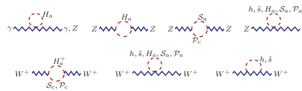
Figure 1: Feynman diagrams for the contributions of the scalar singlet and inert scalar doublets to the oblique electroweak parameters $\Delta S$ and $\Delta T$.

After evaluating them and subtracting the SM contributions, we arrive at

$$6\pi\,\Delta S \,=\,\ln\frac{m_{\mathcal{S}_{1}}m_{\mathcal{S}_{2}}}{m_{H_{1}}m_{H_{2}}}-\frac{5}{6}+\mathrm{cos}^{2}(\theta_{S}+\theta_{P})\,\tilde{F}\big{(}m_{\mathcal{S}_{1}},m_{\mathcal{P}_{1}},m_{\mathcal{S}_{2}},m_{\mathcal{P}_{2}}\big{)}$$

$$~{}~{}~{}~{}~{}+\,\mathrm{sin}^{2}(\theta_{S}+\theta_{P})\,\tilde{F}\big{(}m_{\mathcal{S}_{1}},m_{\mathcal{P}_{2}},m_{\mathcal{S}_{2}},m_{\mathcal{P}_{1}}\big{)}$$

$$~{}~{}~{}~{}~{}+\,s_{\xi}^{2}\Bigg{\{}\frac{m_{\tilde{s}}^{2}-m_{h}^{2}}{4m_{Z}^{2}}+\Bigg{[}\frac{11m_{Z}^{2}-m_{h}^{2}}{\big{(}m_{Z}^{2}-m_{h}^{2}\big{)}\raisebox{1.0pt}{${}^{2}$}}+\frac{1}{m_{Z}^{2}}\Bigg{]}\frac{\mathcal{F}(m_{h},m_{Z})}{2}$$

$$\hskip 40.00006pt-\Bigg{[}\frac{11m_{Z}^{2}-m_{\tilde{s}}^{2}}{\big{(}m_{Z}^{2}-m_{\tilde{s}}^{2}\big{)}\raisebox{1.0pt}{${}^{2}$}}+\frac{1}{m_{Z}^{2}}\Bigg{]}\frac{\mathcal{F}(m_{\tilde{s}},m_{Z})}{2}\Bigg{\}}\,,$$ (61)

$$16\pi m_{W}^{2}s_{\mathrm{w}}^{2}\Delta T \;=\;\mathrm{cos}^{2}(\theta_{H}-\theta_{S})\,\big{(}\mathcal{F}(m_{H_{1}},m_{\mathcal{S}_{1}})+\mathcal{F}(m_{H_{2}},m_{\mathcal{S}_{2}})\big{)}$$

$$~{}~{}~{}~{}~{}+\;\mathrm{sin}^{2}(\theta_{H}-\theta_{S})\,\big{(}\mathcal{F}(m_{H_{1}},m_{\mathcal{S}_{2}})+\mathcal{F}(m_{H_{2}},m_{\mathcal{S}_{1}})\big{)}$$

$$~{}~{}~{}~{}~{}+\;\mathrm{cos}^{2}(\theta_{H}+\theta_{P})\,\big{(}\mathcal{F}(m_{H_{1}},m_{\mathcal{P}_{1}})+\mathcal{F}(m_{H_{2}},m_{\mathcal{P}_{2}})\big{)}$$

$$~{}~{}~{}~{}~{}+\;\mathrm{sin}^{2}(\theta_{H}+\theta_{P})\,\big{(}\mathcal{F}(m_{H_{2}},m_{\mathcal{P}_{1}})+\mathcal{F}(m_{H_{1}},m_{\mathcal{P}_{2}})\big{)}$$

$$~{}~{}~{}~{}~{}-\;\mathrm{cos}^{2}(\theta_{S}+\theta_{P})\,\big{(}\mathcal{F}(m_{\mathcal{S}_{1}},m_{\mathcal{P}_{1}})+\mathcal{F}(m_{\mathcal{S}_{2}},m_{\mathcal{P}_{2}})\big{)}$$

$$~{}~{}~{}~{}~{}-\;\mathrm{sin}^{2}(\theta_{S}+\theta_{P})\,\big{(}\mathcal{F}(m_{\mathcal{S}_{1}},m_{\mathcal{P}_{2}})+\mathcal{F}(m_{\mathcal{P}_{1}},m_{\mathcal{S}_{2}})\big{)}$$

$$~{}~{}~{}~{}~{}+\;3s_{\xi}^{2}\big{(}\mathcal{F}(m_{W},m_{h})-\mathcal{F}(m_{W},m_{\tilde{s}})-\mathcal{F}(m_{Z},m_{h})+\mathcal{F}(m_{Z},m_{\tilde{s}})\big{)}\,,$$ (62)

where

$$\mathcal{F}(m,n) \;=\;\frac{m^{2}+n^{2}}{2}\,-\,\frac{m^{2}n^{2}}{m^{2}-n^{2}}\ln\frac{m^{2}}{n^{2}}\,,$$ (63)

$$\tilde{F}(m_{1},n_{1},m_{2},n_{2}) \;=\;\Bigg{[}\frac{m_{1}^{2}+n_{1}^{2}}{\big{(}m_{1}^{2}-n_{1}^{2}\big{)}\raisebox{1.0pt}{${}^{2}$}}-\frac{1}{m_{1}^{2}}\Bigg{]}\frac{\mathcal{F}\big{(}m_{1},n_{1}\big{)}}{2}+\Bigg{[}\frac{m_{2}^{2}+n_{2}^{2}}{\big{(}m_{2}^{2}-n_{2}^{2}\big{)}\raisebox{1.0pt}{${}^{2}$}}-\frac{1}{m_{2}^{2}}\Bigg{]}\frac{\mathcal{F}\big{(}m_{2},n_{2}\big{)}}{2}$$

$$~{}~{}~{}~{}+\;\frac{n_{1}^{2}}{4m_{1}^{2}}+\frac{n_{2}^{2}}{4m_{2}^{2}}\,,$$ (64)

and hence  $\mathcal{F}(m,m)=0$  and  $\tilde{F}(m,m,n,n)=5/6$.  To check these results, we have also obtained them by employing the formulas provided in Ref. Grimus:2008nb . In our numerical analysis, we apply the $\Delta S$ and $\Delta T$ ranges determined in Ref. pdg .

IV.3 Collider constraints

Based on Eq. (47), we may infer from the measured widths of the $W$ and $Z$ bosons and the absence yet of evidence for non-SM particles in their decay modes that for $a,b=1,2$

$$m_{H_{a}}+m_{\mathcal{S}_{b}}\,>\,m_{W}\,,~{}~{}~{}~{}~{}m_{H_{a}}+m_{\mathcal{P}_{b}}\,>\,m_{W}\,,~{}~{}~{}~{}~{}2m_{H_{a}}\,>\,m_{Z}\,,~{}~{}~{}~{}~{}m_{\mathcal{S}_{a}}+m_{\mathcal{P}_{b}}\,>\,m_{Z}\,.$$ (65)

The null results so far of direct searches for new particles at $e^{+}e^{-}$ colliders also translate into lower limits on these masses, especially those of the charged scalars. In our numerical exploration we will then generally consider the mass regions  $m_{H_{a},\mathcal{S}_{a},\mathcal{P}_{a}}>100$ GeV.

Given that the mixing parameter $c_{\xi}$ defined in Eq. (II) is the rescaling factor of the $h$ couplings to ordinary fermions and weak bosons with respect to their SM counterparts, it needs to satisfy the findings in the LHC experiments that the $h$ couplings cannot deviate by much more than  $\sim$ 10%  from their SM values  atlas+cms . Moreover, for models with a singlet scalar which mixes with the noninert scalar doublet, global fits  Cheung:2015dta to the data yield  $|c_{\xi}|\mbox{\footnotesize\,$\gtrsim$\,}0.86$.  Consequently, we may place the restraint

$$|s_{\xi}|\,<\,0.3\,.$$ (66)

Since the decay  $h\to\gamma\gamma$  has been measured at the LHC, the data imply restrictions on the $H_{1,2}$ contributions to $\Gamma(h\rightarrow\gamma\gamma)$, which we will take into account. On the other hand, although the invisible decay channel of $h$ is also subject to LHC searches, its limit will not apply to our case because the inert scalar masses are chosen to exceed $m_{h}$.

Additional constraints on our scenario come from the fact that searches for new physics in LHC Run 1 did not produce any clear signals of $\tilde{s}$ in its possible decay modes. For the major ones, the data from $pp$ collisions at  $\sqrt{s}=8$ TeV  imply the estimated cross-section limits  pp2s2gg-1

$$\sigma(pp\to\tilde{s}\to\gamma\gamma)_{8\mathrm{\,TeV}}\, \lesssim\,2.3\;\mbox{fb~{}\cite[cite]{\@@bibref{Authors Phrase1YearPhrase2}{Aad:2014ioa,Khachatryan:2015qba}{\@@citephrase{(}}{\@@citephrase{)}}}}\,,$$

$$\sigma(pp\to\tilde{s}\to\gamma Z)_{8\mathrm{\,TeV}}\, \lesssim\,4.0\;\mbox{fb~{}\cite[cite]{\@@bibref{Authors Phrase1YearPhrase2}{Aad:2014fha}{\@@citephrase{(}}{\@@citephrase{)}}}}\,,$$

$$\sigma(pp\to\tilde{s}\to WW)_{8\mathrm{\,TeV}}\, \lesssim\,47\;\mbox{fb~{}\cite[cite]{\@@bibref{Authors Phrase1YearPhrase2}{Aad:2015agg,Khachatryan:2015cwa}{\@@citephrase{(}}{\@@citephrase{)}}}}\,,$$

$$\sigma(pp\to\tilde{s}\to ZZ)_{8\mathrm{\,TeV}}\, \lesssim\,27\;\mbox{fb~{}\cite[cite]{\@@bibref{Authors Phrase1YearPhrase2}{Aad:2015kna}{\@@citephrase{(}}{\@@citephrase{)}}}}\,,$$

$$\sigma(pp\to\tilde{s}\to hh)_{8\mathrm{\,TeV}}\, \lesssim\,41\;\mbox{fb~{}\cite[cite]{\@@bibref{Authors Phrase1YearPhrase2}{ATLAS:2014rxa}{\@@citephrase{(}}{\@@citephrase{)}}}}\,,$$

$$\sigma(pp\to\tilde{s}\to t\bar{t})_{8\mathrm{\,TeV}}\, \lesssim\,700\;\mbox{fb~{}\cite[cite]{\@@bibref{Authors Phrase1YearPhrase2}{Chatrchyan:2013lca}{\@@citephrase{(}}{\@@citephrase{)}}}}\,.$$ (67)

V Constraints on new fermions

The interactions of the Dirac singlet fermions $N_{k}$ with the scalars are described by Eq. (II). The ${\cal Y}_{1,2}$ terms in ${\cal L}_{N}$ are responsible for endowing light neutrinos with masses as well as inducing charged leptons’ flavor-violating transitions and anomalous magnetic moments, all via loop diagrams. As discussed in Appendix  C, the $\hat{\texttt{Y}}_{1,2}$ couplings of $N_{k}$ in Eq. (II) not only cause their chiral components to mix and transform into Majorana particles, but also dictate their interactions with $h$ and $\tilde{s}$. As this transformation involves mixing matrices with unknown elements and our main purpose here is to show that the model possesses a viable candidate for DM, in the following for simplicity we present formulas and results related to $N_{k}$ where the mixing effects can be neglected. Including the latter would only increase the number of free parameters and hence would not alter our basic conclusions.

V.1 Radiative neutrino masses and $\ell\to\ell^{\prime}\gamma$ transitions

The effective Lagrangian for light neutrinos’ Majorana masses has the form

$${\cal L}_{m_{\nu}}\,=\,-\tfrac{1}{2}\,\overline{\nu_{k}^{\rm c}}\,({\cal M}_{\nu})_{kl\,}P_{L}\nu_{l}\;+\;{\rm H.c.}\,,$$ (68)

where  $k,l=1,2,3$  are summed over,  $P_{L}=\tfrac{1}{2}(1-\gamma_{5})$,  and the mass matrix ${\cal M}_{\nu}$ is related to the neutrino eigenmasses $m_{1,2,3}$ by the diagonalization formula  ${\rm diag}\bigl{(}m_{1},m_{2},m_{3}\bigr{)}={\cal U}^{\rm T}{\cal M}_{\nu}\,{\cal U}$  involving the Pontecorvo-Maki-Nakagawa-Sakata (PMNS) unitary matrix $\cal U$. The interactions of the $Z_{2}$-odd fermions and neutral inert scalars given by Eq. (II) provide a mechanism for generating ${\cal M}_{\nu}$ radiatively via one-loop diagrams involving $N_{j}$, ${\cal S}_{a}$, and ${\cal P}_{a}$.

Thus, we obtain

$$({\cal M}_{\nu})_{or} = \frac{({\cal Y}_{1})_{oj}({\cal Y}_{2})_{rj}+({\cal Y}_{2})_{oj}({\cal Y}_{1})_{rj}}{16\pi^{2}}\,M_{j}\Bigg{(}\frac{c_{S}s_{S}\,m_{{\cal S}_{1}}^{2}}{M_{j}^{2}-m_{{\cal S}_{1}}^{2}}\ln\frac{m_{{\cal S}_{1}}^{2}}{M_{j}^{2}}-\frac{c_{S}s_{S}\,m_{{\cal S}_{2}}^{2}}{M_{j}^{2}-m_{{\cal S}_{2}}^{2}}\ln\frac{m_{{\cal S}_{2}}^{2}}{M_{j}^{2}}$$ (69)

$$\hskip 137.77734pt+\;\frac{c_{P}s_{P}\,m_{{\cal P}_{1}}^{2}}{M_{j}^{2}-m_{{\cal P}_{1}}^{2}}\ln\frac{m_{{\cal P}_{1}}^{2}}{M_{j}^{2}}-\frac{c_{P}s_{P}\,m_{{\cal P}_{2}}^{2}}{M_{j}^{2}-m_{{\cal P}_{2}}^{2}}\ln\frac{m_{{\cal P}_{2}}^{2}}{M_{j}^{2}}\Bigg{)},~{}~{}~{}~{}~{}$$

summation over  $j=1,2,3$  being implicit. One notices that the ${\cal M}_{\nu}$ elements are identically zero if one of ${\cal Y}_{1,2}$ is absent or  $s_{S}=s_{P}=0$,  implying that the presence of both $\eta_{1,2}$ is necessary for creating the masses of light neutrinos. However,  $({\cal M}_{\nu})_{kl}=0$  can still happen if  $m_{{\cal S}_{1}}=m_{{\cal S}_{2}}$  and  $m_{{\cal P}_{1}}=m_{{\cal P}_{2}}$  simultaneously.

The $Z_{2}$-odd fermions and $H_{a}^{\pm}$ together give rise to one-loop diagrams responsible for  $\ell\to\ell^{\prime}\gamma$  transitions which are subject to stringent experimental constraints. The diagrams lead us to the branching fraction of the flavor-violating decay  $\ell_{r}\to\ell_{o}\gamma$

$${\cal B}(\ell_{r}\to\ell_{o}\gamma)\,=\,\frac{3\alpha\,{\cal B}(\ell_{r}\to\ell_{o}\nu\bar{\nu})\,v^{4}}{32\pi}\left|\raisebox{2.0pt}{\footnotesize$\displaystyle\sum_{j=1,2,3}$}\Bigg{[}\frac{{\mathbb{C}}_{ojrj}}{m_{H_{1}}^{2}}\;\mathbb{F}\Bigg{(}\frac{M_{j}^{2}}{m_{H_{1}}^{2}}\Bigg{)}+\frac{{\mathbb{C}}_{ojrj}^{\prime}}{m_{H_{2}}^{2}}\;\mathbb{F}\Bigg{(}\frac{M_{j}^{2}}{m_{H_{2}}^{2}}\Bigg{)}\Bigg{]}\right|^{2}$$ (70)

and a contribution to the anomalous magnetic moment $a_{\mu}$ of the muon

$$\delta a_{\mu}\,=\,\frac{-m_{\mu}^{2}}{16\pi^{2}}\,\raisebox{2.0pt}{\footnotesize$\displaystyle\sum_{j=1,2,3}$}\Bigg{[}\frac{{\mathbb{C}}_{2j2j}}{m_{H_{1}}^{2}}\;\mathbb{F}\Bigg{(}\frac{M_{j}^{2}}{m_{H_{1}}^{2}}\Bigg{)}+\frac{{\mathbb{C}}_{2j2j}^{\prime}}{m_{H_{2}}^{2}}\;\mathbb{F}\Bigg{(}\frac{M_{j}^{2}}{m_{H_{2}}^{2}}\Bigg{)}\Bigg{]}\,,$$ (71)

where  $\mathbb{F}(x)=\big{(}1-6x+3x^{2}+2x^{3}-6x^{2}\,\ln x\big{)}/\big{[}6(1-x)^{4}\big{]}$,

$${\mathbb{C}}_{ojrj} \,=\,c_{H}^{2}\big{(}{\cal Y}_{1}\big{)}_{oj}\big{(}{\cal Y}_{1}^{*}\big{)}_{rj}+s_{H}^{2}\big{(}{\cal Y}_{2}\big{)}_{oj}\big{(}{\cal Y}_{2}^{*}\big{)}_{rj}\,,$$

$${\mathbb{C}}_{ojrj}^{\prime} \,=\,s_{H}^{2}\big{(}{\cal Y}_{1}\big{)}_{oj}\big{(}{\cal Y}_{1}^{*}\big{)}_{rj}+c_{H}^{2}\big{(}{\cal Y}_{2}\big{)}_{oj}\big{(}{\cal Y}_{2}^{*}\big{)}_{rj}\,.$$ (72)

Since  $0\leq\mathbb{F}(x)\leq 1/6$  for  $x\geq 0$,  it is obvious from the last two equations that the contribution of the $Z_{2}$-odd particles in this model to $a_{\mu}$ is never positive,  $\delta a_{\mu}\leq 0$.

Experiments have indicated that neutrino masses are tiny and that the room for new physics in  $\ell\to\ell^{\prime}\gamma$  transitions continues to shrink. One can then see from Eqs.  (70) and (71) that the elements of the Yukawa coupling matrices ${\cal Y}_{1,2}$ generally cannot be sizable, unless $M_{j}$ are very large, $\theta_{S,P}$ are small, or fine cancellations occur.

V.2 Fermionic dark matter

We select the lightest mass eigenstate among the singlet fermions to be lighter than all other $Z_{2}$-odd particles, and so it is a candidate for DM. There are many final states into which it can annihilate, depending on its mass, such as  $\ell_{o}^{-}\ell_{r}^{+},\nu_{o}\nu_{r},q\bar{q},W^{+}W^{-},ZZ,hh,h\tilde{s},\tilde{s}\tilde{s}$,  where $q$ is a  quark. The $\ell_{o}^{-}\ell_{r}^{+}$ and $\nu_{o}\nu_{r}$ modes, mostly due to $t$- and $u$-channel diagrams mediated by the inert scalars, are controlled by $({\cal Y}_{1,2})_{j1}$. Although these couplings are not big, they can bring about consequential contributions to the DM annihilation rate, as will be addressed later. Also potentially pertinent are contributions involving the $b\bar{b},W^{+}W^{-},ZZ$, and $t\bar{t}$ final-states and arising at tree level from $h$- and $\tilde{s}$-exchange diagrams in the $s$ channel, which depend on the other Yukawa couplings, $(\hat{\texttt{Y}}_{1,2})_{11}$. The cross sections of some of these processes are relegated to Appendix  C.

Given that direct searches for DM have led to stringent restrictions on the DM interaction with the nucleon, we need to take them into account. In this case, the DM-nucleon scattering proceeds largely from $t$-channel diagrams mediated at tree level by $h$ and $\tilde{s}$. The resulting cross-section is also written down in Appendix  C.

VI Numerical results

Since the $\tilde{s}$ couplings to SM fermions and weak bosons are $s_{\xi}$ times their SM Higgs counterparts, we can estimate the gluon fusion and vector-boson ($W$ and $Z$) fusion contributions to the cross section $\sigma(pp\rightarrow\tilde{s})$ from those of a 750 GeV SM Higgs at  $\sqrt{s}=13$ TeV,  namely  cs8tev ; cs13tev  $\sigma_{g\mathrm{F}}\big{(}pp\rightarrow h_{\mathrm{SM}}^{750}\big{)}=4.693\times 156.8\;\mathrm{fb}\simeq 736\;$fb  and $\sigma_{\mathrm{VBF}}\big{(}pp\rightarrow h_{\mathrm{SM}}^{750}\big{)}=2.496\times 52.35\;\mathrm{fb}\simeq 131\;$fb.  Thus

$$\sigma_{g\mathrm{F+VBF}}(pp\rightarrow\tilde{s})\,=s_{\xi}^{2}\times 867~{}\mathrm{fb}\,.$$ (73)

Another contribution to $\sigma(pp\rightarrow\tilde{s})$ comes from photon fusion  Jaeckel:2012yz ; Csaki:2015vek ; Fichet:2015vvy ; Csaki:2016raa . It has been considered in other studies on this diphoton excess gammaF and can expectedly yield substantial effects if $\mathcal{B}(\tilde{s}\rightarrow\gamma\gamma)$ is sizable. At $\,\sqrt{s}=13\,$TeV,  the cross section of this production mode is  Csaki:2016raa

$$\sigma_{\gamma\mathrm{F}}(pp\rightarrow\tilde{s})\,=\,1.08\times 10^{4}\times\frac{\Gamma_{\tilde{s}}}{45~{}\mathrm{GeV}}\times\mathcal{B}(\tilde{s}\rightarrow\gamma\gamma)~{}\mathrm{fb}\,,$$ (74)

owing to the elastic, partially inelastic, and fully inelastic collisions of the protons, the latter two being dominant  Fichet:2015vvy ; Csaki:2016raa . Therefore, the total production cross-section of $\tilde{s}$ decaying into the diphoton is

$$\sigma(pp\rightarrow\tilde{s}\rightarrow\gamma\gamma)\,=\,\left[\sigma_{g\mathrm{F+VBF}}(pp\rightarrow\tilde{s})+\sigma_{\gamma\mathrm{F}}(pp\rightarrow\tilde{s})\right]\,\times\mathcal{B}(\tilde{s}\rightarrow\gamma\gamma)\,,$$ (75)

where ${\mathcal{B}}(\tilde{s}\to\gamma\gamma)$ is given by Eq. (III).

Employing Eq. (75), we explore the parameter space of the model in order to attain the cross-section level inferred from the ATLAS and CMS reports on the 750 GeV diphoton excess  atlas:s2gg ; cms:s2gg ; Aaboud:2016tru ; Khachatryan:2016hje , namely  pp2s2gg-1

$$\sigma(pp\rightarrow\tilde{s}\rightarrow\gamma\gamma)_{\mathrm{LHC}}\,\sim\,(2-13)~{}\mathrm{fb}\,,$$ (76)

as well as the $\tilde{s}$ total width  $\Gamma_{\tilde{s}}\leq 50$ GeV.  Simultaneously, we take into account the perturbativity, vacuum stability, and unitarity conditions, oblique electroweak parameter tests, and restraints from LHC measurements of  $\mathcal{B}(h\rightarrow\gamma\gamma)$,  as discussed in Sec. IV. Furthermore, we consider the charged scalars’ mass regions  $m_{H_{a}}^{2}>100$ GeV  and let $\tilde{v}$, the VEV of the singlet scalar, vary between 3 and 10  TeV, for  $\tilde{v}<\mathcal{O}$(1 TeV)  would be inadequate for helping enhance the $\tilde{s}\gamma\gamma$ coupling to the right magnitude.

As it turns out, there are viable regions in the model parameter space which satisfy the different requirements. To illustrate this, we present in Fig. 2 the distributions of approximately six thousand randomly-generated benchmark points on the planes of various pairs of quantities. The top left panel shows  $\mathcal{R}_{\gamma\gamma}^{h}=\Gamma(h\rightarrow\gamma\gamma)/\Gamma_{0}(h\rightarrow\gamma\gamma)$  versus  $\mathcal{R}_{\gamma Z}^{h}=\Gamma(h\rightarrow\gamma Z)/\Gamma_{0}(h\rightarrow\gamma Z)$,  where $\Gamma_{0}(h\rightarrow\gamma\gamma,\gamma Z)$ stand for the SM rates and are the same in form as $\Gamma(h\rightarrow\gamma\gamma,\gamma Z)$ in  Eq. (III), respectively, but with  $c_{\xi}=1$  and  $\lambda_{hH_{a}H_{a}}=0$.  Clearly, the model predicts a  positive correlation between $\mathcal{R}_{\gamma\gamma}^{h}$ and $\mathcal{R}_{\gamma Z}^{h}$, which will be testable once the empirical information on  $h\rightarrow\gamma Z$  has become precise enough. In view of the purple (blue) horizontal lines marking the 1$\sigma$ range of $\mathcal{R}_{\gamma\gamma}^{h}$ from ATLAS (CMS) atlas+cms , we expect that many of the predictions which still agree well with the current data will also be tested by upcoming LHC measurements. In addition, using the color guide on the vertical palette accompanying the plot, we see that the preferred values of the mass $m_{H_{1}}$ of the lighter of the charged inert scalars are not far from  $m_{\tilde{s}}/2$.  This is not unexpected because $H_{1}$ with a mass near  $m_{\tilde{s}}/2$  helps maximize the  $\tilde{s}\rightarrow\gamma\gamma$  rate.

The top right and middle panels of Fig. 2 exhibit the distributions on the $m_{H_{1}}$-$m_{H_{2}}$, $m_{\mathcal{S}_{1}}$-$m_{\mathcal{S}_{2}}$, and $m_{\mathcal{P}_{1}}$-$m_{\mathcal{P}_{2}}$ planes. Evidently, all the inert scalars’ masses are greater than $m_{\tilde{s}}/2$, but $m_{H_{1}}$, as already mentioned in the last paragraph, and $m_{\mathcal{S}_{1}}$ do not reach very far away from  $m_{\tilde{s}}/2$, while $m_{\mathcal{P}_{1}}$ can go up to 730 GeV or so. In contrast, the values of $m_{H_{2},\mathcal{S}_{2},\mathcal{P}_{2}}$ lie predominantly in the multi-TeV region, but we also see numerous points corresponding to $m_{H_{2},\mathcal{S}_{2},\mathcal{P}_{2}}$ around or below 1 TeV. For all these masses, the invisible decay channel of $\tilde{s}$ into a pair of inert scalars is of course closed. Based on the accompanying palettes, which provide color guides on the mixing parameters  $s_{H,S,P}^{2}=\mathrm{sin}^{2}\theta_{H,S,P}$,  we deduce that the mixing in each of the three sectors is very suppressed for the majority of the benchmark points, with  $s_{H,S,P}^{2}<10^{-4}$,  whereas for  $m_{H_{2},\mathcal{S}_{2},\mathcal{P}_{2}}\,\mbox{\footnotesize$\leq$}\,\mathcal{O}$(1 TeV)  the mixing can be significant, with $|s_{H,S,P}|$ as high as $\mathcal{O}$(0.5). Recalling Eq. (IV.2) for $\Delta S$ and $\Delta T$, one realizes that these different results on the masses and mixing of the inert scalars comply with the restrictions from electroweak precision data.

​​​​

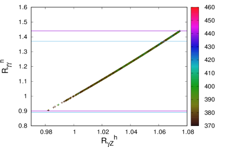
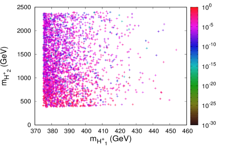
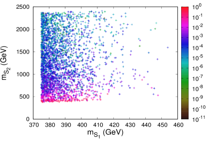
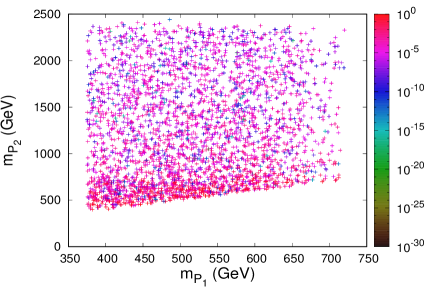
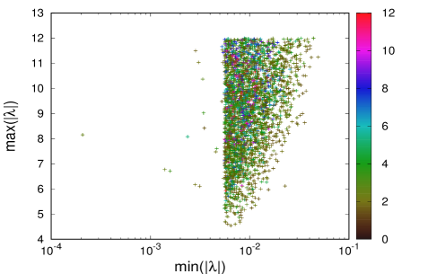
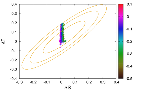
Figure 2: Top left panel: the ratio  $\mathcal{R}_{\gamma\gamma}^{h}=\Gamma(h\rightarrow\gamma\gamma)/\Gamma(h\rightarrow\gamma\gamma)_{\textsc{sm}}$  versus its $\gamma Z$ counterpart; the horizontal lines mark the 1$\sigma$ ranges of $\mathcal{R}_{\gamma\gamma}^{h}$ from ATLAS and CMS atlas+cms ; the palette reads the value of $m_{H_{1}}$ in GeV. Top right and middle panels: the masses of the inert scalars; the palettes read their respective mixing parameters  $s_{H,S,P}^{2}=\mathrm{sin}^{2}\theta_{H,S,P}$.  Bottom left panel: the maximum and minimum magnitudes of the scalars’ quartic couplings $\lambda$s; the palette reads the cross section $\sigma(pp\to\tilde{s}\to\gamma\gamma)$ in  fb. Bottom right panel: the oblique electroweak precision parameters, $\Delta S$ and $\Delta T$; the contours, from smallest to biggest, represent the empirical 68%, 95%, and 99% confidence level, respectively; the palette reads the relative mass difference  $1-(m_{\mathcal{S}_{1}}+m_{\mathcal{P}_{1}})/(2m_{H_{1}})$.

The bottom left panel of Fig. 2 depicts the maximum size of individual quartic scalar couplings versus the minimum size of them, with the palette reading the cross section $\sigma(pp\to\tilde{s}\to\gamma\gamma)$ in  fb. It is obvious that one or more of the couplings need to be fairly large in magnitude, exceeding  6 for most of the benchmarks, which is one of the conditions for the cross section to rise to the desired level. The resulting predictions for $\sigma(pp\to\tilde{s}\to\gamma\gamma)$ appear to lie primarily within the range of 2-7  fb. We also notice that for a preponderance of the points the minimum of the quartic couplings is  $\sim$ 0.005 or higher, which happens to belong to $\lambda_{\zeta}$. In these cases, $m_{\tilde{s}}^{2}$ is chiefly determined by the  $m_{\varsigma}^{2}=\lambda_{\zeta}\tilde{v}^{2}$  contribution, as can be concluded from Eq. (II).

The bottom right panel of Fig. 2 displays the new scalars’ contributions to the oblique electroweak parameters. The plot shows that a substantial fraction of the benchmarks are within the empirical 1$\sigma$ area. With the palette signifying the amount of relative mass splitting  $\hat{\delta}=1-(m_{\mathcal{S}_{1}}+m_{\mathcal{P}_{1}})/(2m_{H_{1}})$  between $H_{1}$ and its lightest neutral counterparts, we also observe that $\Delta S$ has a dependence on $\hat{\delta}$, which is similar to the situation in a newly proposed model involving an inert scalar doublet Ahriche:2016cio .

Before proceeding to the next figure, we would like to remark that the aforesaid tendency of the bulk of $m_{H_{2},\mathcal{S}_{2},\mathcal{P}_{2}}$ values to be in the multi-TeV region is attributable to the necessity for one or more of the scalar quartic couplings and $\tilde{v}$ to be big enough to boost the  $\tilde{s}\rightarrow\gamma\gamma$  rate to the desired amount. On the other hand, $m_{H_{1},\mathcal{S}_{1},\mathcal{P}_{1}}$ have to be fairly close to $m_{\tilde{s}}/2$  and in numerous cases $m_{H_{2},\mathcal{S}_{2},\mathcal{P}_{2}}$ can also be sub-TeV, implying that a degree of fine tuning is unavoidable to achieve such relatively low masses. More precisely, this entails partial cancelation of order $10^{-4}$ or so mainly between the $\mu_{2a}^{2}$ and $\lambda_{a\zeta\,}\tilde{v}^{2}$ parts of $m_{c_{a},n_{a}}^{2}$ in $m_{H_{a},\mathcal{S}_{a},\mathcal{P}_{a}}$, as can be inferred from Eqs.  (24), (42), (80), and (82).

For a closer view on $\sigma(pp\to\tilde{s}\to\gamma\gamma)$, we graph benchmarks for it versus the $\tilde{s}$ total width, $\Gamma_{\tilde{s}}$, in the top left panel of Fig. 3. Obviously, our parameter space of interest can yield a cross section within the empirical range in Eq. (76) and also $\Gamma_{\tilde{s}}$ between $\sim$ 1 and 6  GeV. With the palette reading the fractional value of the combined contribution from gluon fusion and vector-boson fusion, it is clear that in these instances the role of photon fusion is crucial, being responsible for between $\sim$ 80 percent and upper-ninety percent of $\sigma(pp\rightarrow\tilde{s}\rightarrow\gamma\gamma)$.

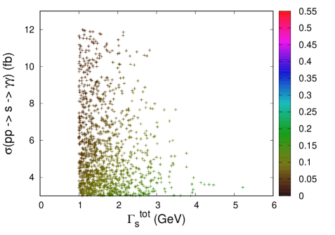
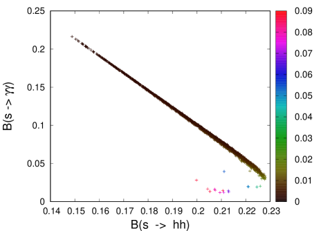
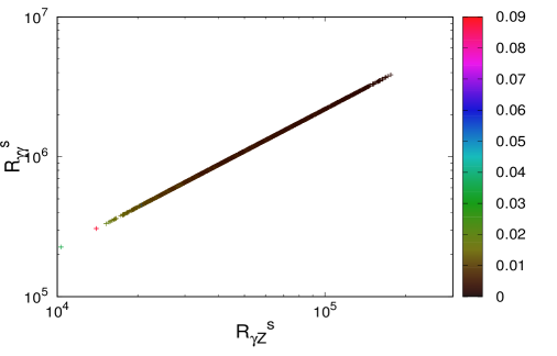
Figure 3: Top left panel: the cross section $\sigma(pp\rightarrow\tilde{s}\rightarrow\gamma\gamma)$ versus the total $\tilde{s}$ width  $\Gamma_{\tilde{s}}=\Gamma_{\tilde{s}}^{\mathrm{tot}}$;  the palette reads the fractional amount of the combined contribution in Eq. (73) from gluon fusion and vector-boson fusion. Top right panel: the branching fractions $\mathcal{B}(\tilde{s}\rightarrow\gamma\gamma)$ and $\mathcal{B}(\tilde{s}\rightarrow hh)$; the palette reads  $s_{\xi}^{2}=\mathrm{sin}^{2}\xi$.  Bottom panel: the ratios $\mathcal{R}_{\gamma\gamma}^{s}$ and $\mathcal{R}_{\gamma Z}^{s}$ of $\Gamma(\tilde{s}\to\gamma\gamma,\gamma Z)$, respectively, to their counterparts without the $H_{1,2}$ contributions; the palette reads $s_{\xi}^{2}$.

Correspondingly, as the top right panel of Fig. 3 reveals, the branching fraction $\mathcal{B}(\tilde{s}\rightarrow\gamma\gamma)$ varies from about 2 to 22 percent, whereas $\mathcal{B}(\tilde{s}\rightarrow hh)$ is mostly between 15 and 23 percent. The substantial $\mathcal{B}(\tilde{s}\rightarrow\gamma\gamma)$ numbers have resulted from the aforementioned big size of one or more of the quartic couplings, $\tilde{v}$ being in the 3-10 TeV range, and the $\tilde{s}\gamma\gamma$ coupling dominated by the $H_{a}$ loop contribution with  $m_{H_{1}}\sim m_{\tilde{s}}/2$  for the majority of the benchmarks.

Still with the same panel, from the palette one can see that the favored mixing between the scalar singlet and noninert doublet is rather small, with  $s_{\xi}^{2}\leq\mathcal{O}$(0.02),  which is expected at least on account of the requirements from electroweak precision data and compatible with results found in very recent literature  Falkowski:2015swt . Accordingly, one can deduce from Eq. (II), for  $m_{\phi}<m_{\varsigma}$,  the approximation  $m_{\tilde{s}}\sim\sqrt{\lambda_{\zeta}}\,\tilde{v}$,  and for our choice of  $\tilde{v}=3$-10  TeV  this causes $\lambda_{\zeta}$ to be quite suppressed, below $\mathcal{O}$(0.06). These findings fit the comments earlier concerning the bottom left panel of Fig. 2.

The bottom panel of Fig. 3 depicts some comparison of  $\tilde{s}\to\gamma\gamma$  and  $\tilde{s}\to\gamma Z$,  particularly  $\mathcal{R}_{\gamma\gamma}^{\tilde{s}}=\Gamma(\tilde{s}\to\gamma\gamma)/\Gamma_{0}(\tilde{s}\to\gamma\gamma)$  versus  $\mathcal{R}_{\gamma Z}^{\tilde{s}}=\Gamma(\tilde{s}\to\gamma Z)/\Gamma_{0}(\tilde{s}\to\gamma Z)$,  with $\Gamma_{0}(\tilde{s}\to\gamma\gamma,\gamma Z)$ being the same in form as $\Gamma(\tilde{s}\to\gamma\gamma,\gamma Z)$ in Eq. (III), respectively, but with  $\lambda_{hH_{a}H_{a}}=0$.  The graph reveals that the $H_{1,2}$ loops can enhance the  $\tilde{s}\to\gamma\gamma,\gamma Z$  rates by several orders of magnitude relative to the case without $H_{1,2}$ and that there is a  positive correlation between $\Gamma(\tilde{s}\to\gamma\gamma,\gamma Z)$, which can be checked experimentally. In addition, for all the benchmarks our computation yields  $\mathcal{R}_{\gamma\gamma}^{\tilde{s}}\simeq 22\,\mathcal{R}_{\gamma Z}^{\tilde{s}}$  as well as  $\Gamma(\tilde{s}\rightarrow\gamma\gamma)\simeq 1.3\,\Gamma(\tilde{s}\rightarrow\gamma Z)$.  The latter translates into  $\sigma(pp\to\tilde{s}\to\gamma\gamma)\simeq 1.3\,\sigma(pp\to\tilde{s}\to\gamma Z)$  and hence constitutes another signature of the model which may also be checked soon at the LHC, as the prediction for $\sigma(pp\to\tilde{s}\to\gamma Z)$ is roughly an order of magnitude below the upper limits recently reported by ATLAS Aaboud:2016trl and CMS CMS:2016ypt .

Other signatures may be accessible by probing  $pp\to\tilde{s}\to hh,W^{+}W^{-},ZZ,t\bar{t}$,  although their cross sections depend on $\xi$ and other parameters. Still, given that  $\mathcal{B}(\tilde{s}\rightarrow hh)=\mathcal{O}$(0.2)  as indicated above, the $hh$ channel is potentially reachable if the $h$ pair can be observed with good precision. Furthermore, since  $\tilde{s}\to W^{+}W^{-},ZZ,t\bar{t}$  have rates adhering to the ratio in Eq. (54), the cross sections of  $pp\to\tilde{s}\to W^{+}W^{-},ZZ,t\bar{t}$  are predicted to obey the same ratio. Therefore, if  $|s_{\xi}|=\mathcal{O}$(0.1),  they may be sufficiently measurable to allow us to test these predictions.

Now, analogously to Eq. (75), at  $\sqrt{s}=8$ TeV  the cross section of  $pp\rightarrow\tilde{s}$  is

$$\sigma(pp\rightarrow\tilde{s})_{8\mathrm{\,TeV}}\, =\,\sigma_{g\mathrm{F+VBF}}(pp\rightarrow\tilde{s})_{8\mathrm{\,TeV}}\,+\,\sigma_{\gamma\mathrm{F}}(pp\rightarrow\tilde{s})_{8\mathrm{\,TeV}}$$ (77)

consisting of the gluon-, vector-boson-, and photon-fusion contributions  cs8tev ; Csaki:2016raa

$$\sigma_{g\mathrm{F+VBF}}(pp\rightarrow\tilde{s})_{8\mathrm{\,TeV}}\, =\,s_{\xi}^{2}\times(156.8+52.35)\mathrm{fb}\,,$$

$$\sigma_{\gamma\mathrm{F}}(pp\rightarrow\tilde{s})_{8\mathrm{\,TeV}}\, =\,5.5\times 10^{3}\times\frac{\Gamma_{\tilde{s}}}{45~{}\mathrm{GeV}}\times\mathcal{B}(\tilde{s}\rightarrow\gamma\gamma)~{}\mathrm{fb}\,.$$ (78)

Using these, we can evaluate  $\sigma_{8}(pp\rightarrow\tilde{s}\rightarrow\mathsf{X})\equiv\sigma(pp\rightarrow\tilde{s})_{8\mathrm{\,TeV\,}}\mathcal{B}(\tilde{s}\rightarrow\mathsf{X})$  in relation to $s_{\xi}^{2}$ for  $\mathsf{X}=\gamma\gamma,\gamma Z,W^{+}W^{-},ZZ,hh,t\bar{t}$  divided by the corresponding experimental limits in Eq. (IV.3). We display the results in Fig. 4. It is evident from this plot that these restraints lead to a  significant decrease in the number of viable points, as a high percentage of the $\gamma\gamma$ benchmarks (in red) resides above the horizontal dotted line. However, currently there is considerable uncertainty in the ratio between the 8 TeV and 13 TeV estimates of the photon-fusion contributions, which could imply a reduction of the first numerical factor in $\sigma_{\gamma\mathrm{F}}(pp\rightarrow\tilde{s})_{8\mathrm{\,TeV}}$ in Eq. (78) by up to twice or more  Fichet:2015vvy ; Csaki:2015vek ; Csaki:2016raa . As a consequence, a substantial portion of the parameter space represented by our scan points may evade the no-signal constraints from the Run 1 searches.

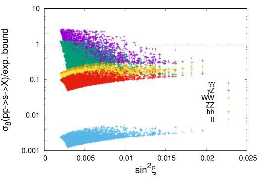
Figure 4: The cross sections of  $pp\rightarrow\tilde{s}\rightarrow\mathsf{X}$  for  $\mathsf{X}=\gamma\gamma,\gamma Z,W^{+}W^{-},ZZ,hh,t\bar{t}$  at the center-of-mass energy  $\sqrt{s}=8$ TeV,  each divided by the corresponding experimental upper-bound from Eq. (IV.3), versus the $\phi$-$\varsigma$ mixing parameter $s_{\xi}^{2}$. Points above the horizontal dotted line are excluded.

Finally, we would like to illustrate how the new fermions $N_{j}$ via the calculated quantities in Eqs. (69)-(71) and Appendix  C are subject to the available experimental data on neutrino masses, the  $\ell\to\ell^{\prime}\gamma$  decays, and the muon anomalous magnetic moment $a_{\mu}$. Assuming $N_{1}$ to be the DM candidate, we take into account as well the constraints from the observed relic abundance and DM direct searches. We employ specifically the results of a recent fit to global neutrino data nudata ,  ${\cal B}(\mu\to e\gamma)<4.2\times 10^{-13}$  from the MEG experiment meg ,  ${\cal B}(\tau\to\mu\gamma)<4.4\times 10^{-8}\;$ and the relic density value  $\Omega\hat{h}^{2}=0.1186\pm 0.0020$  from the Particle Data Group pdg , and the newest upper-limit on DM-nucleon spin-independent elastic cross-section set by the LUX Collaboration lux . Thus, in the same numerical scans as before, we let ${\cal Y}_{a}$, $\big{(}\hat{\texttt{Y}}_{a}\big{)}{}_{11}$, and $M_{j}$ vary within the ranges  $-0.5\leq\mathcal{Y}_{a}\leq 0.5$,   $\big{|}\big{(}\hat{\texttt{Y}}_{1}+\hat{\texttt{Y}}{}_{2}^{*}\big{)}{}_{11}\big{|}\leq 1$,  and  $M_{j}=1$-375  GeV,  with $M_{2,3}$ and also the inert scalar masses being chosen to exceed $1.1\,M_{1}$ to avoid coannihilation effects.

In Fig. 5 we display the results for the absolute values of $\mathcal{Y}_{a}$ and for ${\cal B}(\mu\to e\gamma)$, ${\cal B}(\tau\to\mu\gamma)$, and $|\delta a_{\mu}|$ versus the DM mass, $M_{1}$. Given that $\delta a_{\mu}$ in Eq. (71) is not positive and that the measured and SM values of $a_{\mu}$ presently differ by  $a_{\mu}^{\rm exp}-a_{\mu}^{\textsc{sm}}=(288\pm 80)\times 10^{-11}$ pdg , in the scans we have required $|\delta a_{\mu}|$ to be less than the one-sigma error in this difference,  $|\delta a_{\mu}|<8\times 10^{-10}$.  In  Fig. 6, the left panel depicts the relative contributions of the major DM-annihilation channels  $N_{1}N_{1}\to X$  to the total annihilation rate that satisfies the relic density requirement. Evidently, the $\ell\bar{\ell}^{\prime}$ and $\nu\nu^{\prime}$ contributions, which involve the ${\cal Y}_{1,2}$ elements, are substantial or dominant in the chosen DM mass range, although the other channels, which are controlled by the $\hat{\texttt{Y}}_{1,2}$ elements, can also be important in different mass regions. The right panel of Fig. 6 shows that the predicted DM-nucleon cross-section is well below the latest limit from LUX lux , as $(\hat{\texttt{Y}}{}_{1,2})_{11}$ can be small enough. Clearly, there is still ample room in the model parameter space that is compatible with the existing data.

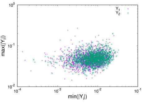
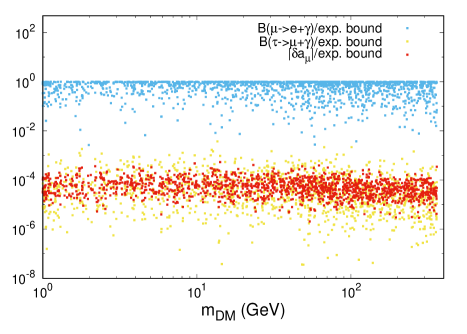
Figure 5: Left: the maximal and minimal values of $|\mathcal{Y}_{1,2}|$ subject to constraints from neutrino oscillation, lepton-flavor violation, and DM data. Right: the predicted ${\cal B}(\mu\to e\gamma)$, ${\cal B}(\tau\to\mu\gamma)$, and $|\delta a_{\mu}|$, normalized by their respective experimental upper-bounds, versus the DM mass,  $m_{\rm DM}=M_{1}$.

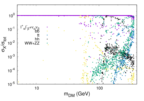
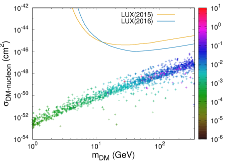
Figure 6: Left: the relative contribution of  $N_{1}N_{1}\to X$  to the DM-annihilation total cross-section corresponding to the observed relic density at freeze-out. Right: the predicted DM-nucleon cross-section versus the DM mass, $M_{1}$, compared to the newest LUX upper-bound lux ; the palette reads the magnitude of $\big{(}\hat{\texttt{Y}}{}_{1}+\hat{\texttt{Y}}{}_{2}^{*}\big{)}{}_{11}$.

VII Conclusions

In this work we have considered the possibility that the observed diphoton excess at an invariant mass of about 750  GeV recently reported by the ATLAS and CMS Collaborations is an indication of a new spinless particle. To explain it, we propose an extension of the SM with a new sector comprising two inert scalar doublets, $\eta_{1,2}$, one scalar singlet, $\zeta$, and three Dirac singlet fermions, $N_{1,2,3}$, all of which transform under a dark Abelian gauge symmetry, U(1)_D. We identify $\tilde{s}$, the heavier one of the mass eigenstates from the mixing of the singlet with the noninert doublet, as the 750 GeV resonance. The inert doublets play an indispensable role because their charged components $H_{1,2}^{\pm}$ can give rise to the loop-induced $\tilde{s}\gamma\gamma$ coupling of the right strength, with suitable choices of the model parameters and without the inclusion of extra colored fermions or bosons. The presence of both inert doublets is also crucial because their components and the singlet fermions together are responsible for endowing light neutrinos with radiative mass. These new scalar doublets and fermions are odd under a $Z_{2}$ symmetry which naturally emerges after the spontaneous breaking of U(1)_D. We choose the lightest mass eigenstate among the singlet fermions to be the lightest $Z_{2}$-odd particle and consequently it can serve as a candidate for DM.

After taking into account the perturbativity condition, the vacuum stability bound, and the constraints from electroweak precision tests, we show that within the allowed parameter space the production cross-section $\sigma(pp\rightarrow\tilde{s}\rightarrow\gamma\gamma)$ can be of order a few fb, mainly due to the sizable contribution from photon fusion in our scenario, while the total width $\Gamma_{\tilde{s}}$ lies in the range of 1-6  GeV. The upcoming data from the LHC with improved precision can be expected to test this prediction for $\Gamma_{\tilde{s}}$. In addition, we point out that the model also predicts roughly similar cross-sections of  $pp\rightarrow\tilde{s}\rightarrow\gamma\gamma,\gamma Z$  and a specific ratio involving the cross-sections of  $pp\rightarrow\tilde{s}\rightarrow W^{+}W^{-},ZZ,t\bar{t}$,  all of which may be experimentally verified in the near future. Lastly, we demonstrate that the interactions of the new fermions can be made to fulfill the restraints from neutrino mass, lepton-flavor violation, muon $g$$-$2, and DM data.

As a final note, after this work was submitted for publication, the ATLAS and CMS Collaborations reported lhc0 that their 2016 data with four times larger statistics than those analyzed in their earlier reports Aaboud:2016tru ; Khachatryan:2016hje revealed no significant diphoton excess above the SM backgrounds at around 750 GeV. Although this does not necessarily rule out the existence of a heavy diphoton resonance, such a particle if existent would have a relatively smaller production cross-section and hence probably require much more statistics to discover. On the other hand, theoretically this implies that it would likely be easier for our model of interest to accommodate the particle, as the scalar couplings and singlet VEV would not need to have the big values seen in our scans. Moreover, as the model parameter space is still considerable, if there is another tentative hint of a heavy diphoton resonance in the future, significantly improved empirical constraints on the various observables discussed above would be needed to probe the model extensively.

Appendix A Scalar masses and couplings

In Eq. (5), the squared-mass matrices $M_{\phi\varsigma,\mathcal{C},0}^{2}$ and column matrix $\eta_{0}$ are given by

$$M_{\phi\varsigma}^{2}\,=\left(\begin{array}[c]{ccc}m_{\phi}^{2}&&\displaystyle\frac{m_{\phi\varsigma}^{2}}{2}\vspace{5pt}\\ \displaystyle\frac{m_{\phi\varsigma}^{2}}{2}&&m_{\varsigma}^{2}\end{array}\right),~{}~{}~{}~{}~{}m_{\phi}^{2}\,=\,\lambda_{1}v^{2}\,,~{}~{}~{}~{}m_{\varsigma}^{2}\,=\,\lambda_{\zeta}\tilde{v}^{2}\,,~{}~{}~{}~{}m_{\phi\varsigma}^{2}\,=\,2\lambda_{3\zeta}^{~{}~{}\;}v\tilde{v}\,,$$ (79)

$$M_{\mathcal{C}}^{2}\,=\left(\begin{array}[c]{ccc}m_{c_{1}}^{2}&&\displaystyle\frac{m_{c\zeta}^{2}}{2}\vspace{5pt}\\ \displaystyle\frac{m_{c\zeta}^{2\ast}}{2}&&m_{c_{2}}^{2}\end{array}\right),~{}~{}~{}~{}~{}m_{c_{a}}^{2}\,=\,\mu_{2a}^{2}+\frac{\lambda_{3a}v^{2}+\lambda_{a\zeta}\tilde{v}^{2}}{2}\,,~{}~{}~{}~{}m_{c\zeta}^{2}\,=\,\sqrt{2}\,\mu_{\eta\zeta\,}\tilde{v}\,,$$ (80)

$$M_{0}^{2}\,=\left(\begin{array}[c]{ccccccc}m_{n_{1}}^{2}&&\displaystyle\frac{m_{n\zeta}^{2}}{2}&&0&&\displaystyle\frac{-\mathrm{Im}\,m_{c\zeta}^{2}}{2}\vspace{5pt}\\ \displaystyle\frac{m_{n\zeta}^{2}}{2}&&m_{n_{2}}^{2}&&\displaystyle\frac{\mathrm{Im}\,m_{c\zeta}^{2}}{2}&&0\vspace{5pt}\\ 0&&\displaystyle\frac{\mathrm{Im}\,m_{c\zeta}^{2}}{2}&&m_{n_{1}}^{2}&&\displaystyle-\frac{\tilde{m}_{n\zeta}^{2}}{2}\vspace{5pt}\\ \displaystyle\frac{-\mathrm{Im}\,m_{c\zeta}^{2}}{2}&&0&&\displaystyle-\frac{\tilde{m}_{n\zeta}^{2}}{2}&&m_{n_{2}}^{2}\end{array}\right),~{}~{}~{}~{}~{}~{}~{}\eta_{0}\,=\left(\begin{array}[c]{c}\mathrm{Re}\,\eta_{1}^{0}\vspace{5pt}\\ \mathrm{Re}\,\eta_{2}^{0}\vspace{5pt}\\ \mathrm{Im}\,\eta_{1}^{0}\vspace{5pt}\\ \mathrm{Im}\,\eta_{2}^{0}\end{array}\right),$$ (81)

$$m_{n_{a}}^{2} \,=\,\mu_{2a}^{2}+\frac{\big{(}\lambda_{3a}+\lambda_{4a}\big{)}v^{2}+\lambda_{a\zeta}\tilde{v}^{2}}{2}\,=\,m_{c_{a}}^{2}+\frac{\lambda_{4a}v^{2}}{2}\,,\vphantom{|_{\int_{\int}^{|}}}$$

$$m_{n\zeta}^{2} \,=\,\frac{\lambda_{5}}{2}\,v^{2}+\mathrm{Re}\,m_{c\zeta}^{2}\,,~{}~{}~{}~{}~{}~{}~{}~{}~{}~{}\tilde{m}_{n\zeta}^{2}\,=\,\frac{\lambda_{5}}{2}\,v^{2}-\mathrm{Re}\,m_{c\zeta}^{2}\,.$$ (82)

The constants $\mu_{2a}^{2}$ enter only these mass formulas of the inert scalars and can be positive or negative if nonzero. To arrive at $M_{\phi\varsigma}^{2}$ in Eq. (79), we have used the relations

$$\mu_{1}^{2}\,=\,\frac{-\lambda_{1\,}v^{2}-\lambda_{3\zeta\,}\tilde{v}^{2}}{2}\,,~{}~{}~{}~{}~{}~{}~{}\mu_{\zeta}^{2}\,=\,\frac{-\lambda_{\zeta\,}\tilde{v}^{2}-\lambda_{3\zeta\,}v^{2}}{2}\,,$$ (83)

corresponding to the vanishing of the first derivatives of the potential $\mathcal{V}$ with respect to $\phi$ and $\varsigma$.

If the parameter $\mu_{\eta\zeta}$ in the potential is complex, so is $M_{\mathcal{C}}^{2}$, which can then be diagonalized with the unitary matrix $\mathcal{U}_{\mathcal{C}}$ according to

$$\mathcal{U}_{\mathcal{C}} \,=\left(\begin{array}[c]{cc}\mathcal{C}_{11}&\mathcal{C}_{12}\vspace{5pt}\\ \mathcal{C}_{21}&\mathcal{C}_{22}\end{array}\!\right)_{\vphantom{|_{\int}^{\int}}},~{}~{}~{}~{}~{}~{}~{}\mathcal{U}_{\mathcal{C}\,}^{\dagger}M_{\mathcal{C}}^{2}\,\mathcal{U}_{\mathcal{C}}\,=\,\mathrm{diag}\bigl{(}m_{H_{1}}^{2},_{\,\!}m_{H_{2}}^{2}\bigr{)}\,,$$ (86)

$$\mathcal{C}_{11} \,=\,\frac{+\mu_{\eta\zeta}}{\sqrt{2}\;\big{|}\mu_{\eta\zeta}\big{|}}\sqrt{1+\frac{m_{c_{2}}^{2}-m_{c_{1}}^{2}}{m_{H_{2}}^{2}-m_{H_{1}}^{2}}}\,=\,\frac{\mu_{\eta\zeta}}{\big{|}\mu_{\eta\zeta}\big{|}\vphantom{|_{\int_{|}^{|}}}}\;\mathcal{C}_{22}\,,$$

$$\mathcal{C}_{12} \,=\,\frac{\mu_{\eta\zeta}}{\sqrt{2}\;\big{|}\mu_{\eta\zeta}\big{|}}\sqrt{1+\frac{m_{c_{1}}^{2}-m_{c_{2}}^{2}}{m_{H_{2}}^{2}-m_{H_{1}}^{2}}}\,=\,\frac{-\mu_{\eta\zeta}}{\big{|}\mu_{\eta\zeta}\big{|}}\;\mathcal{C}_{21}\,.$$ (87)

As noted earlier, without loss of generality, we can select $\mu_{\eta\zeta}$ to be real, rendering $m_{c\zeta}^{2}$ real as well, in which case $\mathcal{U}_{\mathcal{C}}$ has the orthogonal form in Eq. (24).

If $\mu_{\eta\zeta}$ is complex, the matrix $\mathcal{O}_{0}$ that diagonalizes $M_{0}^{2}$ has the form

$$\mathcal{O}_{0}\,=\left(\begin{array}[c]{cccc}\mathcal{N}_{11}&\mathcal{N}_{12}&\mathcal{N}_{13}&\mathcal{N}_{14}\vspace{5pt}\\ \mathcal{N}_{21}&\mathcal{N}_{22}&\mathcal{N}_{23}&\mathcal{N}_{24}\vspace{5pt}\\ \mathcal{N}_{31}&\mathcal{N}_{32}&\mathcal{N}_{33}&\mathcal{N}_{34}\vspace{5pt}\\ \mathcal{N}_{41}&\mathcal{N}_{42}&\mathcal{N}_{43}&\mathcal{N}_{44}\end{array}\right),$$ (92)

where $\mathcal{N}_{rs}$ are mostly complicated. With $\mu_{\eta\zeta}$ being real instead, these elements are much simpler

$$\mathcal{N}_{11} \,=\,\frac{\sigma_{11}\;\mathrm{sgn}\big{(}m_{n\zeta}^{2}\big{)}}{\sqrt{2}}\sqrt{1+\frac{m_{n_{2}}^{2}-m_{n_{1}}^{2}}{m_{\mathcal{S}_{2}}^{2}-m_{\mathcal{S}_{1}}^{2}}}\,,~{}~{}~{}~{}~{}~{}~{}\mathcal{N}_{12}\,=\,\frac{\sigma_{12}}{\sqrt{2}}\sqrt{1+\frac{m_{n_{1}}^{2}-m_{n_{2}}^{2}}{m_{\mathcal{S}_{2}}^{2}-m_{\mathcal{S}_{1}}^{2}}}\,,$$

$$\mathcal{N}_{33} \,=\,\frac{\sigma_{33}\;\mathrm{sgn}\big{(}\tilde{m}_{n\zeta}^{2}\big{)}}{\sqrt{2}}\sqrt{1+\frac{m_{n_{2}}^{2}-m_{n_{1}}^{2}}{m_{\mathcal{P}_{2}}^{2}-m_{\mathcal{P}_{1}}^{2}}}_{\vphantom{|}}^{\vphantom{|}}\,,~{}~{}~{}~{}~{}~{}~{}\mathcal{N}_{34}\,=\,\frac{\sigma_{34}}{\sqrt{2}}\sqrt{1+\frac{m_{n_{1}}^{2}-m_{n_{2}}^{2}}{m_{\mathcal{P}_{2}}^{2}-m_{\mathcal{P}_{1}}^{2}}}\,,$$

$$\vphantom{|_{\int}^{\int}}\mathcal{N}_{22} \,=\,\sigma_{11}\sigma_{12}\,\mathcal{N}_{11}\,,~{}~{}~{}~{}~{}\mathcal{N}_{21}\,=\,-\sigma_{11}\sigma_{12}\,\mathcal{N}_{12}\,,~{}~{}~{}~{}~{}\mathcal{N}_{44}\,=\,-\sigma_{33}\sigma_{34}\,\mathcal{N}_{33}\,,~{}~{}~{}~{}~{}\mathcal{N}_{43}\,=\,\sigma_{33}\sigma_{34}\,\mathcal{N}_{34}\,,$$

$$\vphantom{|_{\int}^{\int}}\mathcal{N}_{13} \,=\,\mathcal{N}_{14}\,=\,\mathcal{N}_{23}\,=\,\mathcal{N}_{24}\,=\,\mathcal{N}_{31}\,=\,\mathcal{N}_{32}\,=\,\mathcal{N}_{41}\,=\,\mathcal{N}_{42}\,=\,0\,,$$

$$\vphantom{|^{\int}}\sigma_{11}^{2} \,=\,\sigma_{12}^{2}\,=\,1\,,~{}~{}~{}~{}~{}~{}~{}\sigma_{33}^{2}\,=\,\sigma_{34}^{2}\,=\,1\,,$$ (93)

where $\sigma_{11,12,33,34}$ are independent of each other and can each be either +1 or $-1$, implying that we can choose  $\sigma_{11}\sigma_{12}=\sigma_{33}\sigma_{34}=+1$  to get the form of $\mathcal{O}_{0}$ in Eq. (42).

The $\lambda$’s in Eq. (52) are

$$\lambda_{hhh}\,=\,3c_{\xi}\left(c_{\xi}^{2}\lambda_{1}+s_{\xi}^{2}\lambda_{3\zeta}\right)-3s_{\xi}\left(c_{\xi}^{2}\lambda_{3\zeta}+s_{\xi}^{2}\lambda_{\zeta}\right)\frac{\tilde{v}}{v}\,,\hskip 70.0001pt$$ (94)

$$\lambda_{hH_{1}H_{1}} =c_{\xi}\left(c_{H}^{2}\lambda_{31}+s_{H}^{2}\lambda_{32}\right)-s_{\xi}\left[\big{(}c_{H}^{2}\lambda_{1\zeta}+s_{H}^{2}\lambda_{2\zeta}\big{)}\frac{\tilde{v}}{v}-\sqrt{2}\,c_{H}s_{H}\,\frac{\mu_{\eta\zeta}}{v}\right],$$

$$\lambda_{hH_{2}H_{2}} =c_{\xi}\left(c_{H}^{2}\lambda_{32}+s_{H}^{2}\lambda_{31}\right)-s_{\xi}\left[\big{(}c_{H}^{2}\lambda_{2\zeta}+s_{H}^{2}\lambda_{1\zeta}\big{)}\frac{\tilde{v}}{v}+\sqrt{2}\,c_{H}s_{H}\,\frac{\mu_{\eta\zeta}}{v}\right],$$ (95)

$$\lambda_{\tilde{s}hh} =c_{\xi}\left[\left(1-3s_{\xi}^{2}\right)\lambda_{3\zeta}+3s_{\xi}^{2}\lambda_{\zeta}\right]+s_{\xi}\left[\left(1-3c_{\xi}^{2}\right)\lambda_{3\zeta}+3c_{\xi}^{2}\lambda_{1}\right]\frac{v}{\tilde{v}}\,,$$ (96)

$$\lambda_{\tilde{s}H_{1}H_{1}} =c_{\xi}\left(c_{H}^{2}\lambda_{1\zeta}+s_{H}^{2}\lambda_{2\zeta}-\sqrt{2}\,c_{H}s_{H}\,\frac{\mu_{\eta\zeta}}{\tilde{v}}\right)+s_{\xi}\big{(}c_{H}^{2}\lambda_{31}+s_{H}^{2}\lambda_{32}\big{)}\frac{v}{\tilde{v}}\,,$$

$$\lambda_{\tilde{s}H_{2}H_{2}} =c_{\xi}\left(c_{H}^{2}\lambda_{2\zeta}+s_{H}^{2}\lambda_{1\zeta}+\sqrt{2}\,c_{H}s_{H}\,\frac{\mu_{\eta\zeta}}{\tilde{v}}\right)+s_{\xi}\big{(}c_{H}^{2}\lambda_{32}+s_{H}^{2}\lambda_{31}\big{)}\frac{v}{\tilde{v}}\,,$$ (97)

$$\lambda_{\tilde{s}{\mathcal{S}}_{1}{\mathcal{S}}_{1}} =c_{\xi}\left(c_{S}^{2}\lambda_{1\zeta}+s_{S}^{2}\lambda_{2\zeta}-\sqrt{2}\,c_{S}s_{S}\,\frac{\mu_{\eta\zeta}}{\tilde{v}}\right)$$

$$+\;s_{\xi}\left[c_{S}^{2}\left(\lambda_{31}+\lambda_{41}\right)+s_{S}^{2}\left(\lambda_{32}+\lambda_{42}\right)-c_{S}s_{S}\,\lambda_{5}\right]\frac{v}{\tilde{v}}\,,\vphantom{|_{\int_{|}^{|}}}$$

$$\lambda_{\tilde{s}{\mathcal{S}}_{2}{\mathcal{S}}_{2}} =c_{\xi}\left(c_{S}^{2}\lambda_{2\zeta}+s_{S}^{2}\lambda_{1\zeta}+\sqrt{2}\,c_{S}s_{S}\,\frac{\mu_{\eta\zeta}}{\tilde{v}}\right)$$

$$+\;s_{\xi}\left[c_{S}^{2}\left(\lambda_{32}+\lambda_{42}\right)+s_{S}^{2}\left(\lambda_{31}+\lambda_{41}\right)+c_{S}s_{S}\,\lambda_{5}\right]\frac{v}{\tilde{v}}\,,\vphantom{|_{\int_{|}^{|}}}$$

$$\lambda_{\tilde{s}{\mathcal{S}}_{1}{\mathcal{S}}_{2}} =c_{\xi}\left[c_{S}s_{S}\left(\lambda_{1\zeta}-\lambda_{2\zeta}\right)+\big{(}c_{S}^{2}-s_{S}^{2}\big{)}\frac{\mu_{\eta\zeta}}{\sqrt{2}\,\tilde{v}}\right]$$

$$+\;s_{\xi}\left[c_{S}s_{S}\left(\lambda_{31}+\lambda_{41}-\lambda_{32}-\lambda_{42}\right)+\tfrac{1}{2}\big{(}c_{S}^{2}-s_{S}^{2}\big{)}\lambda_{5}\right]\frac{v}{\tilde{v}}\,,$$ (98)

$$\lambda_{\tilde{s}{\mathcal{P}}_{1}{\mathcal{P}}_{1}} =c_{\xi}\left(c_{P}^{2}\lambda_{1\zeta}+s_{P}^{2}\lambda_{2\zeta}+\sqrt{2}\,c_{P}s_{P}\,\frac{\mu_{\eta\zeta}}{\tilde{v}}\right)$$

$$+\;s_{\xi}\left[c_{P}^{2}\left(\lambda_{31}+\lambda_{41}\right)+s_{P}^{2}\left(\lambda_{32}+\lambda_{42}\right)-c_{P}s_{P}\,\lambda_{5}\right]\frac{v}{\tilde{v}}\,,\vphantom{|_{\int_{|}^{|}}}$$

$$\lambda_{\tilde{s}{\mathcal{P}}_{2}{\mathcal{P}}_{2}} =c_{\xi}\left(c_{P}^{2}\lambda_{2\zeta}+s_{P}^{2}\lambda_{1\zeta}-\sqrt{2}\,c_{P}s_{P}\,\frac{\mu_{\eta\zeta}}{\tilde{v}}\right)$$

$$+\;s_{\xi}\left[c_{P}^{2}\left(\lambda_{32}+\lambda_{42}\right)+s_{P}^{2}\left(\lambda_{31}+\lambda_{41}\right)+c_{P}s_{P}\,\lambda_{5}\right]\frac{v}{\tilde{v}}\,,\vphantom{|_{\int_{|}^{|}}}$$

$$\lambda_{\tilde{s}{\mathcal{P}}_{1}{\mathcal{P}}_{2}} =c_{\xi}\left[c_{P}s_{P}\left(\lambda_{1\zeta}-\lambda_{2\zeta}\right)-\big{(}c_{P}^{2}-s_{P}^{2}\big{)}\frac{\mu_{\eta\zeta}}{\sqrt{2}\,\tilde{v}}\right]$$

$$+\;s_{\xi}\left[c_{P}s_{P}\left(\lambda_{31}+\lambda_{41}-\lambda_{32}-\lambda_{42}\right)+\tfrac{1}{2}\big{(}c_{P}^{2}-s_{P}^{2}\big{)}\lambda_{5}\right]\frac{v}{\tilde{v}}\,.$$ (99)

We then find

$$\lambda_{hH_{1}H_{1}}+\lambda_{hH_{2}H_{2}} =c_{\xi}\left(\lambda_{31}+\lambda_{32}\right)-s_{\xi}\left(\lambda_{1\zeta}+\lambda_{2\zeta}\right)\frac{\tilde{v}}{v}\,,$$

$$\lambda_{\tilde{s}H_{1}H_{1}}+\lambda_{\tilde{s}H_{2}H_{2}} =c_{\xi}\left(\lambda_{1\zeta}+\lambda_{2\zeta}\right)+s_{\xi}\left(\lambda_{31}+\lambda_{32}\right)\frac{v}{\tilde{v}}\,.$$ (100)

Appendix B Conditions for tree-level unitarity and global minimum of potential

One of the consequential restrictions on the parameters in the scalar potential $\cal V$ is that the amplitudes for scalar-scalar scattering  $s_{1}s_{2}\to s_{3}s_{4}$  at high energies do not violate unitarity. Analogously to the situation in two-Higgs-doublet models Kanemura:1993hm , for the scalar pair  $s_{m}s_{n}$  we can work with the nonphysical components of the scalar doublets and singlet,

$$\Phi\,=\left(\!\begin{array}[]{c}\varphi^{+}\\ \varphi^{0}\end{array}\!\right),~{}~{}~{}~{}\Phi^{\dagger}\,=\,\big{(}\varphi^{-}~{}~{}~{}\varphi^{0*}\big{)}\,,~{}~{}~{}~{}~{}\eta_{a}\,=\left(\!\begin{array}[]{c}\eta_{a}^{+}\vspace{1pt}\\ \eta_{a}^{0}\end{array}\!\right),~{}~{}~{}~{}\eta_{a}^{\dagger}\,=\,\big{(}\eta_{a}^{-}~{}~{}~{}\eta_{a}^{0*}\big{)}\,,~{}~{}~{}~{}~{}\zeta\,,~{}~{}~{}\zeta^{*}\,.$$ (105)

Accordingly, we can select the uncoupled sets of orthonormal pairs

$$\Big{\{}\frac{1}{\sqrt{2}}\,\zeta\zeta\Big{\}}\,,~{}~{}~{}\big{\{}\zeta\eta_{1}^{0}\big{\}}\,,~{}~{}~{}\big{\{}\zeta\eta_{2}^{0*}\big{\}}\,,~{}~{}~{}\Big{\{}\frac{1}{\sqrt{2}}\,\eta_{1}^{0}\eta_{1}^{0}\Big{\}}\,,~{}~{}~{}\big{\{}\zeta\varphi^{0}\big{\}}\,,~{}~{}~{}\big{\{}\eta_{1}^{+}\eta_{2}^{-},\eta_{1}^{0}\eta_{2}^{0*}\big{\}}\,,~{}~{}~{}\Big{\{}\frac{1}{\sqrt{2}}\,\eta_{2}^{0*}\eta_{2}^{0*}\Big{\}}\,,$$

$$\big{\{}\varphi^{+}\eta_{2}^{-},\varphi^{0}\eta_{2}^{0*},\varphi^{-}\eta_{1}^{+},\varphi^{0*}\eta_{1}^{0}\big{\}}\,,~{}~{}~{}\big{\{}\zeta\zeta^{*},\varphi^{+}\varphi^{-},\varphi^{0}\varphi^{0*},\eta_{1}^{+}\eta_{1}^{-},\eta_{1}^{0}\eta_{1}^{0*},\eta_{2}^{+}\eta_{2}^{-},\eta_{2}^{0}\eta_{2}^{0*}\big{\}}\,,$$

$$\big{\{}\varphi^{+}\eta_{1}^{0},\varphi^{0}\eta_{1}^{+}\big{\}}\,,~{}~{}~{}~{}~{}\big{\{}\varphi^{+}\varphi^{0},\eta_{1}^{+}\eta_{2}^{0},\eta_{2}^{+}\eta_{1}^{0}\big{\}}\,,~{}~{}~{}~{}~{}\big{\{}\varphi^{+}\eta_{2}^{0},\varphi^{0}\eta_{2}^{+}\big{\}}$$ (106)

to construct the matrix containing the tree-level amplitudes for  $s_{1}s_{2}\to s_{3}s_{4}$,  which at high energies are dominated by the contributions of four-particle contact diagrams. We can express the distinct eigenvalues of this matrix as

$$\lambda_{\zeta}\,,~{}~{}~{}\lambda_{1\zeta}\,,~{}~{}~{}\lambda_{2\zeta}\,,~{}~{}~{}\lambda_{3\zeta}\,,~{}~{}~{}\lambda_{21}\,,~{}~{}~{}\lambda_{22}\,,~{}~{}~{}\lambda_{31}\pm\lambda_{41}\,,~{}~{}~{}\lambda_{32}\pm\lambda_{42}\,,~{}~{}~{}\lambda_{6}\,,~{}~{}~{}\lambda_{6}+2\lambda_{7}\,,~{}~{}~{}\lambda_{6}-\lambda_{7}\,,$$

$${\cal E}_{\pm}\,=\,\tfrac{1}{2}(\lambda_{31}+\lambda_{32}+2\lambda_{41}+2\lambda_{42})\pm\tfrac{1}{2}\sqrt{(\lambda_{31}-\lambda_{32}+2\lambda_{41}-2\lambda_{42})\raisebox{0.2pt}{${}^{2}$}+9\lambda_{5}^{2}}\,,$$

$$E_{\pm}\,=\,\tfrac{1}{2}(\lambda_{31}+\lambda_{32})\pm\tfrac{1}{2}\sqrt{(\lambda_{31}-\lambda_{32})\raisebox{0.2pt}{${}^{2}$}+\lambda_{5}^{2}}\,,$$

$${\mathbb{E}}_{\pm}\,=\,\tfrac{1}{2}(\lambda_{1}+\lambda_{6}+\lambda_{7})\pm\tfrac{1}{2}\sqrt{(\lambda_{1}-\lambda_{6}-\lambda_{7})\raisebox{0.2pt}{${}^{2}$}+2\lambda_{5}^{2}}\,,$$ (107)

the solutions ${\cal E}_{1,2,3}$ of the cubic polynomial equation

$$0 = {\cal E}^{3}-\big{(}\lambda_{1}+\lambda_{21}+\lambda_{22}\big{)}{\cal E}^{2}+\big{[}\lambda_{1}\big{(}\lambda_{21}+\lambda_{22}\big{)}+\lambda_{21}\lambda_{22}-\lambda_{41}^{2}-\lambda_{42}^{2}-\lambda_{7}^{2}\big{]}{\cal E}$$ (108)

$$+\;\lambda_{1}\big{(}\lambda_{7}^{2}-\lambda_{21}\lambda_{22}\big{)}+\lambda_{21}\lambda_{42}^{2}+\lambda_{22}\lambda_{41}^{2}-2\lambda_{41}\lambda_{42}\lambda_{7}\,,$$

and the solutions $E_{1,2,3,4}$ of the quartic polynomial equation

$$0 = E^{4}-\big{(}3\lambda_{1}+3\lambda_{21}+3\lambda_{22}+2\lambda_{\zeta}\big{)}E^{3}$$ (109)

$$+\;\big{[}\big{(}9\lambda_{1}+6\lambda_{\zeta}\big{)}\big{(}\lambda_{21}+\lambda_{22}\big{)}+9\lambda_{21}\lambda_{22}-(2\lambda_{31}+\lambda_{41})^{2}-(2\lambda_{32}+\lambda_{42})^{2}-(2\lambda_{6}+\lambda_{7})^{2}$$

$$~{}~{}~{}~{}+\,6\lambda_{1}\lambda_{\zeta}-2\big{(}\lambda_{3\zeta}^{2}+\lambda_{1\zeta}^{2}+\lambda_{2\zeta}^{2}\big{)}\big{]}E^{2}$$

$$+\;\big{\{}(3\lambda_{1}+2\lambda_{\zeta})\big{[}(2\lambda_{6}+\lambda_{7})^{2}-9\lambda_{21}\lambda_{22}\big{]}+\big{(}6\lambda_{3\zeta}^{2}-18\lambda_{1}\lambda_{\zeta}\big{)}(\lambda_{21}+\lambda_{22})+6(\lambda_{1}+\lambda_{21})\lambda_{2\zeta}^{2}$$

$$~{}~{}~{}~{}+\,6(\lambda_{1}+\lambda_{22})\lambda_{1\zeta}^{2}-\big{[}2(2\lambda_{31}+\lambda_{41})(2\lambda_{32}+\lambda_{42})+4\lambda_{1\zeta}\lambda_{2\zeta}\big{]}(2\lambda_{6}+\lambda_{7})$$

$$~{}~{}~{}~{}-\,4\big{[}(2\lambda_{31}+\lambda_{41})\lambda_{1\zeta}+(2\lambda_{32}+\lambda_{42})\lambda_{2\zeta}\big{]}\lambda_{3\zeta}+(3\lambda_{21}+2\lambda_{\zeta})(2\lambda_{32}+\lambda_{42})^{2}$$

$$~{}~{}~{}~{}+\,(3\lambda_{22}+2\lambda_{\zeta})(2\lambda_{31}+\lambda_{41})^{2}\big{\}}E$$

$$+\;18\big{[}\lambda_{1}\big{(}\lambda_{21}\lambda_{2\zeta}^{2}-\lambda_{22}\lambda_{1\zeta}^{2}+3\lambda_{21}\lambda_{22}\lambda_{\zeta}\big{)}-\lambda_{21}\lambda_{22}\lambda_{3\zeta}^{2}\big{]}+2(2\lambda_{6}+\lambda_{7})^{2}\big{(}\lambda_{3\zeta}^{2}-3\lambda_{1}\lambda_{\zeta}\big{)}$$

$$+\;12\big{[}\lambda_{21}(2\lambda_{32}+\lambda_{42})\lambda_{2\zeta}+\lambda_{22}(2\lambda_{31}+\lambda_{41})\lambda_{1\zeta}\big{]}\lambda_{3\zeta}-4(2\lambda_{31}+\lambda_{41})(2\lambda_{32}+\lambda_{42})\lambda_{1\zeta}\lambda_{2\zeta}$$

$$+\;2(2\lambda_{31}+\lambda_{41})^{2}\big{(}\lambda_{2\zeta}^{2}-3\lambda_{22}\lambda_{\zeta}\big{)}+2(2\lambda_{32}+\lambda_{42})^{2}\big{(}\lambda_{1\zeta}^{2}-3\lambda_{21}\lambda_{\zeta}\big{)}$$

$$+\;4\big{\{}(2\lambda_{31}+\lambda_{41})(2\lambda_{32}+\lambda_{42})\lambda_{\zeta}-\big{[}(2\lambda_{31}+\lambda_{41})\lambda_{2\zeta}+(2\lambda_{32}+\lambda_{42})\lambda_{1\zeta}\big{]}\lambda_{3\zeta}\big{\}}(2\lambda_{6}+\lambda_{7})$$

$$+\;12\lambda_{1}\lambda_{1\zeta}\lambda_{2\zeta}(2\lambda_{6}+\lambda_{7})\,.$$

The requirement of unitarity dictates that each of these eigenvalues not exceed $8\pi$ in magnitude.

We now discuss how we ensure that the potential minimum with the VEVs of the inert doublets being zero is a global minimum. As usual, we get the possible minima of $\cal V$ from the solutions to

$$\bigg{(}\frac{\partial{\mathcal{V}}}{\partial b}\bigg{)}_{b\,=\langle b\rangle}=\,0\,,~{}~{}~{}~{}~{}\bigg{(}\frac{\partial{\mathcal{V}}}{\partial b^{\dagger}}\bigg{)}_{b\,=\langle b\rangle}=\,0\,,~{}~{}~{}~{}~{}b\,=\,\Phi,\eta_{1},\eta_{2},\zeta\,.$$ (110)

For the VEVs of the multiplets, we adopt the notation

$$\langle\zeta\rangle\,=\,\frac{\tilde{v}}{\sqrt{2}}\,,~{}~{}~{}~{}~{}\langle\Phi\rangle\,=\,\frac{1}{\sqrt{2}}\left(\begin{array}[]{c}0\\ v\\ \end{array}\right),~{}~{}~{}~{}~{}\langle\eta_{1}\rangle\,=\,\frac{1}{\sqrt{2}}\left(\begin{array}[]{c}0\\ v_{1}\\ \end{array}\right),~{}~{}~{}~{}~{}\langle\eta_{2}\rangle\,=\,\frac{1}{\sqrt{2}}\left(\begin{array}[]{c}0\\ v_{2}\\ \end{array}\right),$$ (117)

and so in general $\tilde{v}$, $v$, $v_{1}$, and $v_{2}$ can be zero or nonzero. We have set the charged components of the doublets to zero in order to preserve the electromagnetic $U(1)$ symmetry. To find the minima, we construct the 4$\times$4 Hessian matrix having elements  $\partial^{2}\mathcal{V}/\big{(}\partial b_{m}\partial b_{n}^{\dagger}\big{)}$,  apply to it the solutions to Eq. (110), and require the Hessian to have a positive determinant and positive eigenvalues. The minimum with the desired vacuum pattern

$$\tilde{v}\,\neq\,0\,,~{}~{}~{}~{}~{}~{}~{}v\,\neq\,0\,,~{}~{}~{}~{}~{}~{}~{}v_{1}\,=\,v_{2}\,=\,0$$ (118)

occurs if the parameters in $\cal V$ satisfy the relations in Eq. (83) and the inequality

$$\Big{\{}\Big{[}2\mu_{21}^{2}+(\lambda_{31}+\lambda_{41})v^{2}+\lambda_{1\zeta}\tilde{v}^{2}\Big{]}\Big{[}2\mu_{22}^{2}+(\lambda_{32}+\lambda_{42})v^{2}+\lambda_{2\zeta}\tilde{v}^{2}\Big{]}-2\mu^{2}_{\eta\zeta}\tilde{v}^{2}\Big{\}}$$

$$\;\times\,\Big{\{}\Big{[}2\lambda_{1}v^{2}+\lambda_{3\zeta}\tilde{v}^{2}+2\mu^{2}_{1}\Big{]}\Big{[}\lambda_{3\zeta}v^{2}+2\lambda_{\zeta}\tilde{v}^{2}+2\mu^{2}_{\zeta}\Big{]}-\lambda^{2}_{3\zeta}v^{2}\tilde{v}^{2}\Big{\}}\,>\,0\,.$$ (119)

However, these conditions do not yet guarantee that other minima, with only $v_{1}$ or $v_{2}$ being zero or with none of the VEVs being zero, are not lower. The corresponding expressions in these other cases are lengthy and hence not shown here. Therefore, to make sure that Eq. (118) corresponds to the absolute minimum of $\cal V$, in numerical simulations we check that the parameter values yield the lowest $\cal V$ among the different minima, as well as meet all other requirements.

Appendix C Masses and interactions of new fermions

From ${\cal L}_{N}$ in Eq. (II), we can express the terms responsible for the new fermions’ masses as

$${\cal L}_{N}\,\supset\,{\cal L}_{N}^{\prime}\,=\,-\tfrac{1}{2}\Big{(}\overline{(N_{R})\raisebox{1.0pt}{${}^{\rm c}$}}~{}~{}~{}~{}~{}\overline{N_{L}}\Big{)}\left(\!\begin{array}[]{cc}\sqrt{2}\,\tilde{v}\,\hat{\texttt{Y}}_{1}&M_{N}^{\rm T}\vspace{2pt}\\ M_{N}&\sqrt{2}\,\tilde{v}\,\hat{\texttt{Y}}_{2}\end{array}\!\right)\left(\!\begin{array}[]{c}N_{R}\vspace{3pt}\\ (N_{L})\raisebox{1.0pt}{${}^{\rm c}$}\end{array}\!\right)+\;{\rm H.c.}$$ (124)

This implies that in the presence of $\hat{\texttt{Y}}_{1,2}$ the left- and right-handed components of $N_{k}$ mix, leading to Majorana mass eigenstates ${\texttt{N}}_{k,L}$ and ${\mathtt{N}}_{k,R}$ which in general have different masses. In terms of the latter,

$${\cal L}_{N}^{\prime} = -\tfrac{1}{2}\Big{[}\overline{{\mathtt{N}}_{L}}\,\hat{m}_{L}\,({\mathtt{N}}_{L})\raisebox{1.0pt}{${}^{\rm c}$}+\overline{({\mathtt{N}}_{R})\raisebox{1.0pt}{${}^{\rm c}$}}\,\hat{m}_{R}\,{\mathtt{N}}_{R}\Big{]}\,+\,{\rm H.c.}\,,~{}~{}~{}~{}~{}~{}~{}\left(\!\begin{array}[]{c}N_{R}\vspace{2pt}\\ (N_{L})\raisebox{1.0pt}{${}^{\rm c}$}\end{array}\!\right)=\,\mathbb{U}\left(\!\begin{array}[]{c}{\mathtt{N}}_{R}\vspace{2pt}\\ ({\mathtt{N}}_{L})\raisebox{1.0pt}{${}^{\rm c}$}\end{array}\!\right),$$ (129)

$$\mathbb{U} = \left(\!\begin{array}[]{cc}U_{RR}&U_{RL}\vspace{1pt}\\ U_{LR}&U_{LL}\end{array}\!\right),~{}~{}~{}~{}~{}~{}~{}\left(\!\begin{array}[]{cc}\hat{m}_{R}&0\vspace{1pt}\\ 0&\hat{m}_{L}\end{array}\!\right)=\,{\mathbb{U}}^{\rm T}\left(\!\begin{array}[]{cc}\sqrt{2}\,\tilde{v}\,\hat{\texttt{Y}}_{1}&M_{N}^{\rm T}\vspace{1pt}\\ M_{N}&\sqrt{2}\,\tilde{v}\,\hat{\texttt{Y}}_{2}\end{array}\!\right){\mathbb{U}}\,,$$ (136)

where $\mathbb{U}$ is a unitary 6$\times$6 matrix, $U_{LL,LR,RL,RR}$ denote its 3$\times$3 submatrices, and $\hat{m}_{L,R}$ are each diagonal 3$\times$3 matrices for the eigenmasses. Hence  $U_{LL,RR}\to\openone$  and  $U_{LR,RL}\to 0$  if $\hat{\texttt{Y}}_{1,2}$ are negligible or vanishing. It follows that the interactions of these fermions with the scalars are described by

$${\cal L}_{N} \supset \overline{\ell_{\,}}\big{[}\big{(}c_{H}{\cal Y}_{1}U_{RR}-s_{H}{\cal Y}_{2}U_{LR}\big{)}H_{1}^{-}+\big{(}s_{H}{\cal Y}_{1}U_{RR}+c_{H}{\cal Y}_{2}U_{LR}\big{)}H_{2}^{-}\big{]}{\mathtt{N}}_{R}$$ (140)

$$\!+\;\overline{\ell_{\,}}\big{[}\big{(}c_{H}{\cal Y}_{1}U_{RL}-s_{H}{\cal Y}_{2}U_{LL}\big{)}H_{1}^{-}+\big{(}s_{H}{\cal Y}_{1}U_{RL}+c_{H}{\cal Y}_{2}U_{LL}\big{)}H_{2}^{-}\big{]}({\mathtt{N}}_{L})^{\rm c}$$

$$\!-\;\tfrac{1}{\sqrt{2}}\,\overline{\nu}\big{[}\big{(}c_{S}{\cal Y}_{1}U_{RR}-s_{S}{\cal Y}_{2}U_{LR}\big{)}{\cal S}_{1}+\big{(}s_{S}{\cal Y}_{1}U_{RR}+c_{S}{\cal Y}_{2}U_{LR}\big{)}{\cal S}_{2}\big{]}{\mathtt{N}}_{R}$$

$$\!-\;\tfrac{1}{\sqrt{2}}\,\overline{\nu}\big{[}\big{(}c_{S}{\cal Y}_{1}U_{RL}-s_{S}{\cal Y}_{2}U_{LL}\big{)}{\cal S}_{1}+\big{(}s_{S}{\cal Y}_{1}U_{RL}+c_{S}{\cal Y}_{2}U_{LL}\big{)}{\cal S}_{2}\big{]}({\mathtt{N}}_{L})^{\rm c}$$

$$\!+\;\tfrac{i}{\sqrt{2}}\,\overline{\nu}\big{[}\big{(}c_{P}{\cal Y}_{1}U_{RR}+s_{P}{\cal Y}_{2}U_{LR}\big{)}{\cal P}_{1}+\big{(}s_{P}{\cal Y}_{1}U_{RR}-c_{P}{\cal Y}_{2}U_{LR}\big{)}{\cal P}_{2}\big{]}{\mathtt{N}}_{R}$$

$$\!+\;\tfrac{i}{\sqrt{2}}\,\overline{\nu}\big{[}\big{(}c_{P}{\cal Y}_{1}U_{RL}-s_{P}{\cal Y}_{2}U_{LL}\big{)}{\cal P}_{1}+\big{(}s_{P}{\cal Y}_{1}U_{RL}+c_{P}{\cal Y}_{2}U_{LL}\big{)}{\cal P}_{2}\big{]}({\mathtt{N}}_{L})^{\rm c}$$

$$\!+\;\frac{s_{\xi}h-c_{\xi}\tilde{s}}{\footnotesize\mbox{$\sqrt{2}$}}\!\!\begin{array}[t]{l}\Big{[}\overline{({\mathtt{N}}_{R})\raisebox{1.0pt}{${}^{\rm c}$}}\big{(}U_{RR}^{\rm T}\hat{\texttt{Y}}_{1}U_{RR}+U_{LR}^{\rm T}\hat{\texttt{Y}}_{2}U_{LR}\big{)}{\mathtt{N}}_{R}-2\,\overline{{\mathtt{N}}_{L}}\big{(}U_{RL}^{\rm T}\hat{\texttt{Y}}_{1}U_{RR}+U_{LL}^{\rm T}\hat{\texttt{Y}}_{2}U_{LR}\big{)}{\mathtt{N}}_{R}\\ \;+~{}\overline{{\mathtt{N}}_{L}}\big{(}U_{RL}^{\rm T}\hat{\texttt{Y}}_{1}U_{RL}+U_{LL}^{\rm T}\hat{\texttt{Y}}_{2}U_{LL}\big{)}({\mathtt{N}}_{L})\raisebox{1.0pt}{${}^{\rm c}$}\Big{]}\end{array}$$

$$\!+\;{\rm H.c.}$$

Among the important contributions to the DM annihilation rate are those with lepton pairs, $\ell\bar{\ell}^{\prime}$ or $\nu\nu^{\prime}$, in the final state which are dominated by tree-level contributions from diagrams mediated by the inert scalars in the $t$ and $u$ channels. If the effects of $\hat{\texttt{Y}}_{1,2}$ can be neglected, we take $N_{1}$ to be the DM. The cross section of  $N_{1}N_{1}\to\ell_{o}^{-}\ell_{r}^{+}$  is then

$$\sigma_{N_{1}N_{1}\to\ell_{o}\bar{\ell}_{r}} = \frac{1}{32\pi\big{(}s-4M_{1}^{2}\big{)}}\Bigg{\{}\Bigg{[}\frac{c_{H}^{2}s_{H}^{2}{\tt L}_{1}}{{\cal M}_{1}^{2}+\tfrac{1}{2}s}+\frac{c_{H}^{2}s_{H}^{2}{\tt L}_{2}}{{\cal M}_{2}^{2}+\tfrac{1}{2}s}+\frac{\big{(}c_{H}^{4}+s_{H}^{4}\big{)}({\tt L}_{1}+{\tt L}_{2})}{{\cal M}_{1}^{2}+{\cal M}_{2}^{2}+s}\Bigg{]}M_{1}^{2}\,{\rm Re}\big{(}{\cal Y}_{t}^{2*}Y_{u}^{2}\big{)}$$ (141)

$$\hskip 70.0001pt+\;c_{H}^{2}s_{H}^{2}\big{(}|{\cal Y}_{t}|^{4}+|{\cal Y}_{u}|^{4}\big{)}\Bigg{(}\sqrt{1-\frac{4M_{1}^{2}}{s}}+\frac{{\cal M}_{1}^{4}\,{\tt L}_{1}-{\cal M}_{2}^{4}\,{\tt L}_{2}}{m_{H_{1}}^{2}s-m_{H_{2}}^{2}s}\Bigg{)}$$

$$\hskip 70.0001pt+\;\big{(}c_{H}^{4}|{\cal Y}_{t}|^{4}+s_{H}^{4}|{\cal Y}_{u}|^{4}\big{)}{\mathbb{R}}_{1}+\big{(}s_{H}^{4}|{\cal Y}_{t}|^{4}+c_{H}^{4}|{\cal Y}_{u}|^{4}\big{)}{\mathbb{R}}_{2}\Bigg{\}}\,,$$

where

$${\tt L}_{a} = \ln\frac{2{\cal M}_{a}^{2}+s-\sqrt{s^{2}-4M_{1}^{2}s}}{2{\cal M}_{a}^{2}+s+\sqrt{s^{2}-4M_{1}^{2}s}}\;,~{}~{}~{}~{}~{}~{}~{}{\cal Y}_{t}^{2}\,=\,({\cal Y}_{1})_{o1}({\cal Y}_{1})_{r1}^{*}\,,~{}~{}~{}~{}~{}~{}~{}{\cal Y}_{u}^{2}\,=\,({\cal Y}_{2})_{o1}({\cal Y}_{2})_{r1}^{*}\,$$

$${\cal M}_{a}^{2} = m_{H_{a}}^{2}-M_{1}^{2}\,,~{}~{}~{}~{}~{}~{}~{}{\mathbb{R}}_{a}\,=\,\frac{{\cal M}_{a}^{4}+\tfrac{1}{2}\,m_{H_{a}}^{2}s}{{\cal M}_{a}^{4}+m_{H_{a}}^{2}s}\,\sqrt{1-\frac{4M_{1}^{2}}{s}}+\frac{{\cal M}_{a}^{2}}{s}\,{\tt L}_{a}\,.$$ (142)

For  $o=r$,  there are also contributions from $h$- and $\tilde{s}$-mediated diagrams in the $s$ channel, but these are suppressed by $m_{\ell_{o}}/v$ and hence can be ignored. The cross section of  $N_{1}N_{1}\to\nu_{o}\nu_{r}$,  arising from ${\cal S}_{1,2}$- and ${\cal P}_{1,2}$-exchange diagrams, is much lengthier and not displayed here.

Also potentially important are the channels  $N_{1}N_{1}\to(h^{*},\tilde{s}^{*})\to X_{\mathrm{SM}}=b\bar{b},W^{+}W^{-},ZZ,t\bar{t}$,  each of which has a cross section

$$\sigma_{N_{1}N_{1}\to(h^{*},\tilde{s}^{*})\to X_{\mathrm{SM}}} = \frac{c_{\xi}^{2}s_{\xi}^{2}}{2}\Big{\{}\big{(}s-2M_{1}^{2}\big{)}\Big{[}\big{|}\big{(}\hat{\texttt{Y}}_{1}\big{)}{}_{11}\big{|}^{2}+\big{|}\big{(}\hat{\texttt{Y}}_{2}\big{)}{}_{11}\big{|}^{2}\Big{]}+4M_{1}^{2}\,{\rm Re}\Big{[}\big{(}\hat{\texttt{Y}}_{1}\big{)}_{11}\big{(}\hat{\texttt{Y}}_{2}\big{)}_{11}\Big{]}\Big{\}}$$ (143)

$$\times\;\bigg{|}\frac{1}{s-m_{h}^{2}+i\Gamma_{h}m_{h}}-\frac{1}{s-m_{\tilde{s}}^{2}+i\Gamma_{\tilde{s}}m_{\tilde{s}}}\bigg{|}^{2}~{}\frac{\Gamma_{h_{\mathrm{SM}}\to X_{\mathrm{SM}}}\big{|}_{m_{h}^{2}=s}}{\sqrt{s-4M_{1}^{2}}}\,.$$

We have also looked at  $N_{1}N_{1}\to hh$,  but its contribution turns out to be unimportant in our parameter space of interest.

The scattering of $N_{1}$ off a nucleon $\cal N$ at tree level is mediated by $h$ and $\tilde{s}$. The cross section in the nonrelativistic limit is

$$\sigma_{\rm DM\mbox{-}nucleon}\;=\;\frac{c_{\xi}^{2}s_{\xi}^{2}\,g_{{\cal NN}h\,}^{2}M_{1}^{2}m_{\cal N}^{2}\,\Big{|}\big{(}\hat{\texttt{Y}}_{1}\big{)}_{11}+\big{(}\hat{\texttt{Y}}_{2}^{*}\big{)}_{11}\Big{|}^{2}}{2\pi\,\big{(}M_{1}+m_{\cal N}\big{)}\raisebox{1.0pt}{${}^{2}$}}\bigg{(}\frac{1}{m_{h}^{2}}-\frac{1}{m_{\tilde{s}}^{2}}\bigg{)}^{\!2}\,,$$ (144)

where the effective Higgs-nucleon coupling  $g_{{\cal NN}h}=0.0011$  is at the lower end of its range estimated in Ref. He:2011gc and thus helps minimize the prediction in light of the strict experimental limits.

References

- (1) ATLAS Collaboration, ATLAS-CONF-2015-081.
- (2) CMS Collaboration, CMS-PAS-EXO-15-004.
- (3) M. Aaboud et al. [ATLAS Collaboration], arXiv:1606.03833 [hep-ex].
- (4) V. Khachatryan et al. [CMS Collaboration], arXiv:1606.04093 [hep-ex].
- (5) M. Backovic et al., arXiv:1512.04917; S. Knapen et al., arXiv:1512.04928; D. Buttazzo et al., arXiv:1512.04929; R. Franceschini et al., arXiv:1512.04933; S. Di Chiara et al., arXiv:1512.04939; J. Ellis et al., arXiv:1512.05327; M. Low et al., arXiv:1512.05328; A. Kobakhidze et al., arXiv:1512.05585; A. Ahmed et al., arXiv:1512.05771; W. Altmannshofer et al., arXiv:1512.07616.
- (6) S. Sun, arXiv:1411.0131; A. Biswas and A. Lahiri, arXiv:1511.07159; K. Harigaya and Y. Nomura, Phys. Lett. B 754, 151 (2016) [arXiv:1512.04850]; Y. Mambrini et al., arXiv:1512.04913; A. Angelescu et al., arXiv:1512.04921; Y. Nakai et al., arXiv:1512.04924; A. Pilaftsis, Phys. Rev. D 93, no. 1, 015017 (2016) [arXiv:1512.04931]; B. Bellazzini et al., arXiv:1512.05330; R.S. Gupta et al., arXiv:1512.05332; E. Molinaro et al., arXiv:1512.05334; S.D. McDermott et al., arXiv:1512.05326; C. Petersson and R. Torre, arXiv:1512.05333; B. Dutta et al., arXiv:1512.05439; P. Cox et al., arXiv:1512.05618; A. Ahmed et al., arXiv:1512.05771; P. Agrawal et al., arXiv:1512.05775; D. Becirevic et al., arXiv:1512.05623; J.M. No et al., arXiv:1512.05700; S.V. Demidov and D.S. Gorbunov, arXiv:1512.05723; W. Chao et al., arXiv:1512.05738; D. Curtin and C.B. Verhaaren, arXiv:1512.05753; L. Bian et al., arXiv:1512.05759; J. Chakrabortty et al., arXiv:1512.05767; D. Aloni et al., arXiv:1512.05778; Y. Bai et al., arXiv:1512.05779; S. Ghosh et al., arXiv:1512.05786; E. Gabrielli et al., Phys. Lett. B 756, 36 (2016) [arXiv:1512.05961]; J.S. Kim et al., arXiv:1512.06083; A. Alves et al., arXiv:1512.06091; E. Megias et al., arXiv:1512.06106; J. Bernon and C. Smith, arXiv:1512.06113; W. Chao, arXiv:1512.06297; A. Ringwald and K. Saikawa, arXiv:1512.06436; M.T. Arun and P. Saha, arXiv:1512.06335; C. Han et al., arXiv:1512.06376; S. Chang, arXiv:1512.06426; X.F. Han and L. Wang, Phys. Rev. D 93, no. 5, 055027 (2016) [arXiv:1512.06587]; H. Han et al., arXiv:1512.06562; M.x. Luo et al., arXiv:1512.06670; J. Chang et al., arXiv:1512.06671; D. Bardhan et al., arXiv:1512.06674; T.F. Feng et al., arXiv:1512.06696; M. Dhuria and G. Goswami, arXiv:1512.06782; W.S. Cho et al., arXiv:1512.06824; D. Barducci et al., arXiv:1512.06842; M. Chala et al., Phys. Lett. B 755, 145 (2016) [arXiv:1512.06833]; I. Chakraborty and A. Kundu, arXiv:1512.06508; R. Ding et al., arXiv:1512.06560; H. Hatanaka, arXiv:1512.06595; O. Antipin et al., arXiv:1512.06708; F. Wang et al., arXiv:1512.06715; J. Cao et al., arXiv:1512.06728; F.P. Huang et al., arXiv:1512.06732; X.J. Bi et al., arXiv:1512.06787; J.S. Kim et al., arXiv:1512.06797; J.M. Cline and Z. Liu, arXiv:1512.06827; K. Kulkarni, arXiv:1512.06836; S.M. Boucenna et al., arXiv:1512.06878; P.S.B. Dev and D. Teresi, arXiv:1512.07243; J. de Blas et al., arXiv:1512.07229; C.W. Murphy, arXiv:1512.06976; A.E.C. Hernandez and I. Nisandzic, arXiv:1512.07165; U.K. Dey et al., arXiv:1512.07212; G.M. Pelaggi et al., arXiv:1512.07225; Q.H. Cao et al., arXiv:1512.07541; J. Gu and Z. Liu, arXiv:1512.07624; W.C. Huang et al., arXiv:1512.07268; M. Chabab et al., arXiv:1512.07280; S. Moretti and K. Yagyu, arXiv:1512.07462; K.M. Patel and P. Sharma, arXiv:1512.07468; M. Badziak, arXiv:1512.07497; S. Chakraborty et al., arXiv:1512.07527; M. Cvetic et al., arXiv:1512.07622; B.C. Allanach et al., arXiv:1512.07645; K. Das and S.K. Rai, arXiv:1512.07789; H. Davoudiasl and C. Zhang, arXiv:1512.07672; J. Liu et al., arXiv:1512.07885; J. Zhang and S. Zhou, arXiv:1512.07889; L.J. Hall et al., arXiv:1512.07904; H. Han et al., arXiv:1512.07992; J.C. Park and S.C. Park, arXiv:1512.08117; D. Chway et al., arXiv:1512.08221; H. An et al., arXiv:1512.08378; F. Wang et al., arXiv:1512.08434; Q.H. Cao et al., arXiv:1512.08441; J. Gao et al., arXiv:1512.08478; P.S.B. Dev et al., JHEP02, 186 (2016) [arXiv:1512.08507]; L. Del Debbio et al., arXiv:1512.08242; A. Salvio and A. Mazumdar, Phys. Lett. B 755, 469 (2016) [arXiv:1512.08184]; G. Li et al., arXiv:1512.08255; M. Son and A. Urbano, arXiv:1512.08307; Y.L. Tang and S.h. Zhu, arXiv:1512.08323; J. Cao et al., arXiv:1512.08392; C. Cai et al., arXiv:1512.08440; J.E. Kim, Phys. Lett. B 755, 190 (2016) [arXiv:1512.08467]; W. Chao, arXiv:1512.08484; X.J. Bi et al., arXiv:1512.08497; L.A. Anchordoqui et al., Phys. Lett. B 755, 312 (2016) [arXiv:1512.08502]; N. Bizot et al., arXiv:1512.08508; Y. Hamada et al., arXiv:1512.08984; A. Pich, Acta Phys. Polon. B 47, 151 (2016) [arXiv:1512.08749]; L.E. Ibanez and V. Martin-Lozano, arXiv:1512.08777; C.W. Chiang et al., arXiv:1512.08895; S.K. Kang and J. Song, arXiv:1512.08963; S. Kanemura et al., arXiv:1512.09048; S. Kanemura et al., arXiv:1512.09053; P.V. Dong and N.T.K. Ngan, arXiv:1512.09073; I. Low and J. Lykken, arXiv:1512.09089; A.E.C. Hernandez, arXiv:1512.09092; Y. Jiang et al., arXiv:1512.09127; K. Kaneta et al., arXiv:1512.09129; L. Marzola et al., JHEP 1603, 190 (2016) [arXiv:1512.09136]; E. Ma, arXiv:1512.09159; arXiv:1601.01400; A. Dasgupta et al., arXiv:1512.09202; S. Jung et al., arXiv:1601.00006; X.F. Han et al., Phys. Lett. B 756, 309 (2016) [arXiv:1601.00534]; P. Ko et al., arXiv:1601.00586; C.T. Potter, arXiv:1601.00240; E. Palti, arXiv:1601.00285; H.J. Kang and W. Wang, arXiv:1601.00373; K. Ghorbani and H. Ghorbani, arXiv:1601.00602; U. Danielsson et al., arXiv:1601.00624; W. Chao, arXiv:1601.00633; T. Modak et al., arXiv:1601.00836; B. Dutta et al., arXiv:1601.00866; A.E.C. Hernandez et al., arXiv:1601.00661; H. Ito et al., arXiv:1601.01144; H. Zhang, arXiv:1601.01355; A. Berlin, arXiv:1601.01381; S. Bhattacharya et al., arXiv:1601.01569; D. Borah et al., arXiv:1601.01828; N. Sonmez, arXiv:1601.01837; L.G. Xia, arXiv:1601.02454; P. Ko and T. Nomura, arXiv:1601.02490; J. Cao et al., arXiv:1601.02570; M.T. Arun and D. Choudhury, arXiv:1601.02321; C. Hati, arXiv:1601.02457; J.H. Yu, arXiv:1601.02609; R. Ding et al., arXiv:1601.02714; Z. Fodor et al., arXiv:1601.03302; J.H. Davis et al., arXiv:1601.03153; L.V. Laperashvili et al., Int. J. Mod. Phys. A 31, 1650029 (2016) [arXiv:1601.03231]; I. Dorsner et al., arXiv:1601.03267; A. Djouadi et al., arXiv:1601.03696; A.E. Faraggi and J. Rizos, arXiv:1601.03604; L.A. Harland-Lang et al., arXiv:1601.03772; T. Appelquist et al., arXiv:1601.04027; D. Bardhan et al., arXiv:1601.04165; A. Ghoshal, arXiv:1601.04291; T. Nomura and H. Okada, arXiv:1601.04516; W. Chao, arXiv:1601.04678; M.R. Buckley, arXiv:1601.04751; X.F. Han et al., Phys. Lett. B 757, 537 (2016) [arXiv:1601.04954]; H. Okada and K. Yagyu, arXiv:1601.05038; D.B. Franzosi and M.T. Frandsen, arXiv:1601.05357; A. Martini et al., arXiv:1601.05729; C.W. Chiang and A.L. Kuo, arXiv:1601.06394; U. Aydemir and T. Mandal, arXiv:1601.06761; V. Branchina et al., arXiv:1601.06963; J. Kawamura and Y. Omura, arXiv:1601.07396; M.J. Dolan et al., arXiv:1601.07208; B.J. Kavanagh, arXiv:1601.07330; C.Q. Geng and D. Huang, arXiv:1601.07385; E. Bertuzzo et al., arXiv:1601.07508; I. Ben-Dayan and R. Brustein, arXiv:1601.07564; T. Robens and T. Stefaniak, arXiv:1601.07880; F. del Aguila et al., arXiv:1602.00126; L. Aparicio et al., arXiv:1602.00949; R. Ding et al., arXiv:1602.00977; K. Harigaya and Y. Nomura, arXiv:1602.01092; T. Li et al., arXiv:1602.01377; A. Salvio et al., arXiv:1602.01460; S.F. Ge et al., arXiv:1602.01801; S.I. Godunov et al., arXiv:1602.02380; S.B. Giddings and H. Zhang, arXiv:1602.02793; U.K. Dey and T. Jha, arXiv:1602.03286; U. Ellwanger and C. Hugonie, arXiv:1602.03344; K. J. Bae et al., arXiv:1602.03653; C. Arbelaez et al., arXiv:1602.03607; C. Han et al., arXiv:1602.04204; Y. Hamada et al., arXiv:1602.04170; B. Dasgupta et al., arXiv:1602.04692; C. Delaunay and Y. Soreq, arXiv:1602.04838; Y.J. Zhang et al., arXiv:1602.05539; P.S.B. Dev et al., arXiv:1602.05947; F. Staub et al., arXiv:1602.05581; S. Baek and J.h. Park, arXiv:1602.05588; M. Cvetic et al., arXiv:1602.06257; A. Kobakhidze, arXiv:1602.06363; S. De Curtis et al., arXiv:1602.06437; D.K. Hong and D.H. Kim, arXiv:1602.06628; C. Quigg, arXiv:1602.07020; M. Redi et al., arXiv:1602.07297; D.N. Dinh et al., arXiv:1602.07437; J. Ren and J. H. Yu, arXiv:1602.07708; C.W. Chiang et al., arXiv:1602.07909; F. Domingo et al., arXiv:1602.07691; C. Han et al., arXiv:1602.08100; B.A. Arbuzov and I.V. Zaitsev, arXiv:1602.08293; T. Nomura et al., arXiv:1602.08302; Y. Kats and M. Strassler, arXiv:1602.08819; C. Beskidt et al., arXiv:1602.08707; T. Li et al., arXiv:1602.09099; M. He et al., arXiv:1603.00287; Y. Tsai et al., arXiv:1603.00024; R. Barbieri et al., arXiv:1603.00718; M. Backovic, arXiv:1603.01204; C.Y. Chen et al., arXiv:1603.01256.
- (7) A. Falkowski et al., JHEP 1602, 152 (2016) [arXiv:1512.05777]; K. Cheung et al., arXiv:1512.07853.
- (8) S. Fichet et al., arXiv:1512.05751.
- (9) C. Csaki et al., Phys. Rev. D 93, no. 3, 035002 (2016) [arXiv:1512.05776].
- (10) C. Csaki et al., arXiv:1601.00638.
- (11) L. Berthier et al., arXiv:1512.06799; J. A. Casas et al., arXiv:1512.07895; T. Nomura and H. Okada, Phys. Lett. B 755, 306 (2016) [arXiv:1601.00386]; F. D’Eramo et al., arXiv:1601.01571; I. Sahin, arXiv:1601.01676; S. Fichet et al., arXiv:1601.01712; M. Fabbrichesi and A. Urbano, arXiv:1601.02447; S. Abel and V. V. Khoze, arXiv:1601.07167; L. A. Harland-Lang et al., arXiv:1601.07187. T. Nomura and H. Okada, arXiv:1601.07339; A. D. Martin and M. G. Ryskin, J. Phys. G 43, 04 (2016) [arXiv:1601.07774]; N. D. Barrie et al., Phys. Lett. B 755, 343 (2016) [arXiv:1602.00475]; C. Gross et al., arXiv:1602.03877; C. Frugiuele et al., arXiv:1602.04822; P. Ko et al., arXiv:1602.07214; E. Molinaro et al., arXiv:1602.07574.
- (12) V. Keus, S.F. King, and S. Moretti, JHEP 1401, 052 (2014) [arXiv:1310.8253 [hep-ph]].
- (13) E. Ma, I. Picek, and B. Radovcić, Phys. Lett. B 726, 744 (2013) [arXiv:1308.5313 [hep-ph]].
- (14) A. Ahriche, G. Faisel, S.Y. Ho, S. Nasri, and J. Tandean, Phys. Rev. D 92, no. 3, 035020 (2015) [arXiv:1501.06605 [hep-ph]].
- (15) G. Aad et al. [ATLAS and CMS Collaborations], Phys. Rev. Lett. 114, 191803 (2015) [arXiv: 1503.07589 [hep-ex]].
-
(16)
S. Heinemeyer et al. [LHC Higgs Cross Section Working Group
Collaboration],
arXiv:1307.1347 [hep-ph].
Online updates available at
https://twiki.cern.ch/twiki/bin/view/LHCPhysics/CERNYellowReportPageBR2014. - (17) C.S. Chen, C.Q. Geng, D. Huang, and L.H. Tsai, Phys. Rev. D 87, 075019 (2013) [arXiv:1301.4694 [hep-ph]].
- (18) S. Kanemura, T. Kasai, and Y. Okada, Phys. Lett. B 471, 182 (1999) [hep-ph/9903289].
- (19) M.E. Peskin and T. Takeuchi, Phys. Rev. D 46, 381 (1992).
- (20) K.A. Olive et al. [Particle Data Group Collaboration], Chin. Phys. C 38, 090001 (2014) and 2015 update.
- (21) W. Grimus, L. Lavoura, O.M. Ogreid, and P. Osland, Nucl. Phys. B 801, 81 (2008) [arXiv:0802.4353 [hep-ph]].
- (22) The ATLAS and CMS Collaborations, ATLAS-CONF-2015-044 and CMS-PAS-HIG-15-002.
- (23) K. Cheung, P. Ko, J.S. Lee, and P.Y. Tseng, JHEP 1510, 057 (2015) [arXiv:1507.06158 [hep-ph]].
- (24) G. Aad et al. [ATLAS Collaboration], Phys. Rev. Lett. 113, no. 17, 171801 (2014) [arXiv:1407.6583[hep-ex]].
- (25) V. Khachatryan et al. [CMS Collaboration], Phys. Lett. B 750, 494 (2015) [arXiv:1506.02301 [hep-ex]].
- (26) G. Aad et al. [ATLAS Collaboration], Phys. Lett. B 738, 428 (2014) [arXiv:1407.8150 [hep-ex]].
- (27) G. Aad et al. [ATLAS Collaboration], JHEP 1601, 032 (2016) [arXiv:1509.00389 [hep-ex]].
- (28) V. Khachatryan et al. [CMS Collaboration], JHEP 1510, 144 (2015) [arXiv:1504.00936 [hep-ex]].
- (29) G. Aad et al. [ATLAS Collaboration], Eur. Phys. J. C 76, no. 1, 45 (2016) [arXiv:1507.05930 [hep-ex]].
- (30) ATLAS Collaboration, ATLAS-CONF-2014-005.
- (31) S. Chatrchyan et al. [CMS Collaboration], Phys. Rev. Lett. 111, no. 21, 211804 (2013) [Phys. Rev. Lett. 112, no. 11, 119903 (2014)] [arXiv:1309.2030 [hep-ex]].
- (32) https://twiki.cern.ch/twiki/bin/view/LHCPhysics/CERNYellowReportPageAt8TeV2014.
- (33) https://twiki.cern.ch/twiki/bin/view/LHCPhysics/CERNYellowReportPageAt1314TeV2014.
- (34) J. Jaeckel, M. Jankowiak, and M. Spannowsky, Phys. Dark Univ. 2, 111 (2013) [arXiv:1212.3620 [hep-ph]].
- (35) A. Ahriche, K.L. McDonald, and S. Nasri, arXiv:1604.05569 [hep-ph].
- (36) M. Aaboud et al. [ATLAS Collaboration], arXiv:1607.06363 [hep-ex].
- (37) CMS Collaboration, CMS-PAS-EXO-16-020; CMS-PAS-EXO-16-021.
- (38) M.C. Gonzalez-Garcia, M. Maltoni, and T. Schwetz, JHEP 1411, 052 (2014) [arXiv:1409.5439]. Online updates available at http://www.nu-fit.org.
- (39) A.M. Baldini et al. [MEG Collaboration], Eur. Phys. J. C 76, no. 8, 434 (2016) [arXiv:1605.05081 [hep-ex]].
- (40) D.S. Akerib et al., arXiv:1608.07648 [astro-ph.CO].
- (41) ATLAS Collaboration, ATLAS-CONF-2016-059; V. Khachatryan et al. [CMS Collaboration], [arXiv:1609.02507 [hep-ex]].
- (42) S. Kanemura, T. Kubota, and E. Takasugi, Phys. Lett. B 313, 155 (1993) [hep-ph/9303263]; A.G. Akeroyd, A. Arhrib, and E.M. Naimi, Phys. Lett. B 490, 119 (2000) [hep-ph/0006035].
- (43) X.G. He, B. Ren, and J. Tandean, Phys. Rev. D 85, 093019 (2012) [arXiv:1112.6364 [hep-ph]].