Phase Retrieval of Real-Valued Signals in a Shift-Invariant Space

Abstract

Phase retrieval arises in various fields of science and engineering and it is well studied in a finite-dimensional setting. In this paper, we consider an infinite-dimensional phase retrieval problem to reconstruct real-valued signals living in a shift-invariant space from its phaseless samples taken either on the whole line or on a set with finite sampling rate. We find the equivalence between nonseparability of signals in a linear space and its phase retrievability with phaseless samples taken on the whole line. For a spline signal of order $N$, we show that it can be well approximated, up to a sign, from its noisy phaseless samples taken on a set with sampling rate $2N-1$. We propose an algorithm to reconstruct nonseparable signals in a shift-invariant space generated by a compactly supported continuous function $\phi$. The proposed algorithm is robust against bounded sampling noise and it could be implemented in a distributed manner.

I Introduction

Phase retrieval plays important roles in signal/image/speech processing ([1]–[9]). It reconstructs a signal of interest from its magnitude measurements. The underlying recovery problem is possible to be solved only if we have additional information about the signal.

The phase retrieval problem of finite-dimensional signals has received considerable attention in recent years ([10]–[14]). In the finite-dimensional setting, a fundamental problem in phase retrieval is whether and how a vector ${\bf x}\in{\mathbb{R}}^{d}$ (or ${\mathbb{C}}^{d}$) can be reconstructed from its magnitude measurements ${\bf y}=|{\bf A}{\bf x}|$, where ${\bf A}$ is a measurement matrix. The phase retrievability has been fully characterized via the measurement matrix ${\bf A}$ ([10, 14, 15]), and many algorithms have been proposed to reconstruct the vector ${\bf x}$ from its magnitude measurements ${\bf y}$ ([1, 8, 12, 13, 16, 17, 18]).

The phase retrieval problem in an infinite-dimensional space is fundamentally different from a finite-dimensional setting. There are several papers devoted to that topic ([19]–[26]). Thakur proved in [19] that real-valued bandlimited signals could be reconstructed from their phaseless samples taken at more than twice the Nyquist rate. The above result was extended to complex-valued bandlimited signals by Pohl, Yang and Boche in [22] with samples taken at more than four times the Nyquist rate. Recently, the phase retrievability of signals living in a principal shift-invariant space was studied by Shenoy, Mulleti and Seelamantula in [24] when only magnitude measurements of their frequency are available.

Shift-invariant spaces have been widely used in sampling theory, wavelet theory, approximation theory and signal processing, see [27]–[31] and references therein. In this paper, we consider the phase retrieval problem for real-valued signals in a principal shift-invariant space

$$V(\phi):=\Big{\{}\sum_{k\in{\mathbb{Z}}}c(k)\phi(t-k):\ c(k)\in{\mathbb{R}}\Big{\}},$$ (I.1)

where the generator $\phi$ is a real-valued continuous function with compact support. Our model of the generator $\phi$ is the B-spline $B_{N}$ of order $N\geq 1$, which is obtained by convoluting the indicator function $\chi_{[0,1)}$ on the unit interval $N$ times,

$$B_{N}=\underbrace{\chi_{[0,1)}*\cdots*\chi_{[0,1)}}_{N}.$$ (I.2)

I-A Contribution

In this paper, we show in Theorem II.2 that a real-valued signal $f\in V(\phi)$ is determined, up to a sign, from its magnitude $|f(t)|,t\in{\mathbb{R}}$, if and only if $f$ is nonseparable, i.e., it is not the sum of two nonzero signals in $V(\phi)$ with their supports being essentially disjoint. As an application of Theorem II.2, we conclude that for any shift-invariant space $V(\phi)$ with continuous generator $\phi$ having compact support, not all signals in $V(\phi)$ could be determined, up to a sign, from its magnitude $|f(t)|,t\in{\mathbb{R}}$, cf. [19, Theorem 1] for the shift-invariant space generated by the sinc function $\frac{\sin\pi t}{\pi t}$.

Phase retrieval in a shift-invariant space is a nonlinear sampling and reconstruction problem ([32, 33, 34]). In this paper, we show in Theorem II.6 and Corollary II.7 that a nonseparable spline signal in $V(B_{N})$ is determined, up to a sign, from its phaseless samples taken on the shift-invariant set

$$Y_{1}:=X+{\mathbb{Z}},$$ (I.3)

where $N\geq 2$ and $X$ contains $2N-1$ distinct points in $(0,1)$.

The set $Y_{1}$ in (I.3) has sampling rate $2N-1$, which is larger than the sampling rate needed for the phase retrievability of band-limited signals [19, Theorem 1]. Let

$$N=\min_{N_{2},N_{1}\in{\mathbb{Z}}}\{N_{2}-N_{1},\phi\ {\rm vanishes\ outside}\ [N_{1},N_{2}]\}$$ (I.4)

be the support length of the generator $\phi$, which is the same as the order $N$ for the B-spline generator $B_{N}$. A natural question is whether any nonseparable signal in the shift-invariant space $V(\phi)$ can be reconstructed from its phaseless samples taken on a set with sampling rate less than $2N-1$. From Example III.3 we see that any nonseparable linear spline signal in $V(B_{2})$ can be determined, up to a sign, from its phaseless samples taken on the set $(\{x_{1},x_{2}\}+{\mathbb{Z}})\cup\{x_{3}\}$ with sampling rate $2$, where $x_{1},x_{2},x_{3}$ are three distinct points in $(0,1)$. In Theorem III.4, we consider the phase retrieval problem of a nonseparable signal in the shift-invariant space $V(\phi)$ from its phaseless samples taken on a nonuniform set

$$Y_{\infty}:=X\cup(\Gamma+{\mathbb{Z}}_{+})\cup(\Gamma^{*}+{\mathbb{Z}}_{-})$$ (I.5)

with sampling rate $N$, where ${\mathbb{Z}}_{\pm}$ is the set of all positive/negative integers, and the sets $\Gamma=\{\gamma_{1},\ldots,\gamma_{N}\}$ and $\Gamma^{*}=\{\gamma_{1}^{*},\ldots,\gamma_{N}^{*}\}$ are contained in $X=\{x_{1},\ldots,x_{2N-1}\}\subset(0,1)$.

Stability of phase retrieval is of central importance. The reader may refer to [15, 35, 36, 37] for phase retrieval in finite-dimensional setting and [38] for nonlinear frames. In this paper, we consider the scenario that phaseless samples taken on a sampling set

$$Y_{L}=\Big{(}X\cup\Big{\{}\Gamma+l,\Gamma^{\ast}-l^{\prime}:1\leq l,l^{\prime}\leq\frac{L-1}{2}\Big{\}}\Big{)}+L{\mathbb{Z}}$$ (I.6)

are corrupted,

$$z_{\boldsymbol{\epsilon}}(y)=|f(y)|^{2}+{\boldsymbol{\epsilon}}(y),\ y\in Y_{L},$$

where $L$ is an odd integer, $f$ is a nonseparable signal in $V(\phi)$, and additive noises ${\boldsymbol{\epsilon}}=({\boldsymbol{\epsilon}}(y))_{y\in Y_{L}}$ have the noise level $|{\boldsymbol{\epsilon}}|=\sup\{|{\boldsymbol{\epsilon}}(y)|:\ y\in Y_{L}\}$. In Theorem IV.1, we establish the stability of phase retrieval in the above scenario.

The set $Y_{L}$ in (I.6) has sampling rate $N+(N-1)/L$. It becomes the shift-invariant set $X+{\mathbb{Z}}$ in (I.3) for $L=1$. Then as an application of Theorem IV.1, any nonseparable spline signal in $V(B_{N})$ can be reconstructed, up to a sign, approximately from its noisy phaseless samples on $X+{\mathbb{Z}}$. The nonuniform sampling set $Y_{\infty}$ in (I.5) can be interpreted as the limit of the sets $Y_{L}$ as $L$ tends to infinity. Due to the exponential decay requirement (IV.29) about $L$ on the noise level, we cannot obtain from Theorem IV.1 that any nonseparable signal in the shift-invariant space $V(\phi)$ could be well approximated, up to a sign, when only its noisy phaseless samples on the nonuniform set $Y_{\infty}$ are available.

Many algorithms have been proposed to solve the phase retrieval problem in finite-dimensional setting ([1, 8, 12, 13, 16, 17, 18]). In this paper, we propose the MEPS algorithm to find an approximation $f_{\boldsymbol{\epsilon}}$ of a nonseparable signal $f\in V(\phi)$ when its noisy phaseless samples $(z_{\boldsymbol{\epsilon}}(y))_{y\in Y_{L}}$ are available. The MEPS algorithm contains four steps: minimization, extension, phase adjustment and sewing. Our numerical simulations indicate that the MEPS algorithm is robust against bounded additive noises ${\boldsymbol{\epsilon}}$, and the error between the reconstructed signal $f_{\boldsymbol{\epsilon}}$ and the original signal $f$ is $O(\sqrt{|\boldsymbol{\epsilon}|})$.

I-B Organization

The paper is organized as follows. In Section II, we characterize the phase retrievability of a real-valued signal $f$ in a linear space from its magnitude $|f(t)|,t\in{\mathbb{R}}$. We also provide several equivalent statements for the phase retrievability of a signal in the shift-invariant space $V(\phi)$ when its phaseless samples on the shift-invariant set $X+{\mathbb{Z}}$ in (I.3) are available only. In Section III, we present an illustrative example of the phase retrieval problem for linear spline signals, and we prove that any nonseparable signal $f$ in the shift-invariant space $V(\phi)$ could be determined, up to a sign, from its phaseless samples $|f(t)|$ taken on the nonuniform sampling set $Y_{\infty}$ in (I.5). In Section IV, we propose the MEPS algorithm to reconstruct a nonseparable signal in $V(\phi)$ from its noisy phaseless samples on $Y_{L}$ in (I.6), and we use it to establish the stability of the phase retrieval problem. In Section V, we present some simulations to demonstrate the stability of the proposed MEPS algorithm. Even though the stability requirement (IV.29) in Theorem IV.1 is not met for large $L$, the MEPS algorithm still has high success rate to save phases of nonseparable signals in $V(\phi)$. All proofs are included in appendices.

II Phase retrievability and nonseparability

In this section, we consider the problem when a signal $f$ in a shift-invariant space can be recovered, up to a sign, from its magnitude measurements $|f(t)|,t\in S$, where $S$ is either the whole line ${\mathbb{R}}$ or a shift-invariant set $X+{\mathbb{Z}}$.

Definition II.1.

Let $V$ be a linear space of real-valued continuous signals on the real line ${\mathbb{R}}$. A signal $f\in V$ is said to be separable if there exist nonzero signals $f_{1}$ and $f_{2}$ in $V$ such that

$$f=f_{1}+f_{2}\ \ {\rm and}\ \ f_{1}f_{2}=0.$$ (II.1)

The set of all nonseparable signals in $V$ contains the zero signal. It is a cone of $V$ but not a convex set in general. A separable signal $f\in V$ is the sum of two nonzero signals $f_{1}$ and $f_{2}\in V$ with their supports being essentially disjoint. Then it cannot be recovered, up to a sign, from its magnitude measurements $|f|$, since $|f|=|f_{1}+f_{2}|=|f_{1}-f_{2}|$ and $f\neq\pm(f_{1}-f_{2})$. In the following theorem, we show that the converse is true.

Theorem II.2.

Let $V$ be a linear space of real-valued continuous signals on the real line ${\mathbb{R}}$. Then a signal $f\in V$ is determined, up to a sign, by its magnitude measurements $|f(t)|,t\in{\mathbb{R}}$, if and only if $f$ is nonseparable.

Observe that all bandlimited signals are nonseparable, as they are analytic on the real line. Therefore, by Theorem II.2, we have the following result about bandlimited signals, cf. [19, Theorem 1].

Corollary II.3.

Any real-valued bandlimited signal is determined, up to a sign, by its magnitude measurements on the real line.

Let $\phi$ be a real-valued generator of the shift-invariant space $V(\phi)$, and $N$ be its support length given in (I.4). Without loss of generality, we assume that

$$\phi(t)=0\ {\rm for\ all}\ t\not\in[0,N],$$ (II.2)

otherwise replacing $\phi$ by $\phi(\cdot-N_{0})$ for some $N_{0}\in{\mathbb{Z}}$. Clearly, $\phi(t)-\phi(t-N)$ is a separable signal in $V(\phi)$. Then from Theorem II.2 we obtain

Corollary II.4.

Let $\phi$ be a continuous function with compact support. Then not all signals $f$ in $V(\phi)$ can be determined, up to a sign, by their magnitude measurements $|f(t)|,t\in{\mathbb{R}}$.

Next, we discuss the nonseparability of signals in a shift-invariant space $V(\phi)$. For the case that $N=1$ (i.e., the generator $\phi$ is supported on $[0,1]$), one may verify that a signal $f\in V(\phi)$ is nonseparable if and only if there exists an integer $k_{0}$ such that

$$f(t)=c({k_{0}})\phi(t-k_{0})\ \ {\rm for\ some}\ \ c({k_{0}})\in{\mathbb{R}}.$$ (II.3)

This implies that any nonseparable signal in $V(\phi)$ can be recovered, up to a sign, from its phaseless samples taken on the shift-invariant set $t_{0}+{\mathbb{Z}}$, where $t_{0}\in(0,1)$ is so chosen that $\phi(t_{0})\neq 0$. So, from now on, we consider the phase retrieval problem only for signals in $V(\phi)$ with the support length $N$ of the generator $\phi$ satisfying

$$N\geq 2.$$ (II.4)

Before characterizing the nonseparability (and hence phase retrievability by Theorem II.2) of signals in a shift-invariant space, let us consider nonseparability of piecewise linear signals.

Example II.5.

Due to the interpolation property of the B-spline $B_{2}$ of order $2$, piecewise linear signals $f\in V(B_{2})$ have the following expansion,

$$f(t)=\sum_{k\in{\mathbb{Z}}}f(k+1)B_{2}(t-k).$$

Therefore $f\in V(B_{2})$ is separable if and only if there exist integers $k_{0}<k_{1}<k_{2}$ such that $f(k_{0})f(k_{2})\neq 0$ and $f(k_{1})=0$. Thus the separable signal

$$f=\hskip-5.78172pt\sum_{k\leq k_{1}-2}f(k+1)B_{2}(t-k)+\hskip-2.168pt\sum_{k\geq k_{1}}f(k+1)B_{2}(t-k)=:f_{1}+f_{2},$$

is the sum of two nonzero signals $f_{1},f_{2}\in V(B_{2})$ supported in $(-\infty,k_{1}]$ and $[k_{1},\infty)$ respectively.

In the following theorem, we extend the support separation property in Example II.5 to separable signals in a shift-invariant space.

Theorem II.6.

Let $\phi$ be a real-valued continuous function satisfying (II.2) and (II.4), $X:=\{x_{m},1\leq m\leq 2N-1\}\subset(0,1)$, and let $f(t)=\sum_{k\in{\mathbb{Z}}}c(k)\phi(t-k)$ be a nonzero real-valued signal in $V(\phi)$. If all $N\times N$ submatrices of

$$\Phi=\big{(}\phi(x_{m}+n)\big{)}_{1\leq m\leq 2N-1,0\leq n\leq N-1}$$ (II.5)

are nonsingular, then the following statements are equivalent.

• The signal $f$ is nonseparable.

• $\sum_{l=0}^{N-2}|c({k+l})|^{2}\neq 0$ for all $K_{-}(f)-N+1<k<K_{+}(f)+1$, where $K_{-}(f)=\inf\{k,c(k)\neq 0\}$ and $K_{+}(f)=\sup\{k,c(k)\neq 0\}$.

• The signal $f$ is determined, up to a sign, from its phaseless samples $|f(t)|,t\in X+{\mathbb{Z}}$, taken on the shift-invariant set $X+{\mathbb{Z}}$.

The nonsingularity of $N\times N$ submatrices of the matrix $\Phi$ in (II.5), i.e., $\|(\Phi_{N})^{-1}\|<\infty$, is also known as its full sparkness ([39, 40]), where

$$\hskip-1.4457pt\|(\Phi_{N})^{-1}\| \hskip-5.78172pt= \hskip-5.78172pt\sup_{1\leq m_{0}<\ldots<m_{N-1}\leq 2N-1}$$ (II.6)

$$\Big{\|}\Big{(}\big{(}\phi(x_{m_{l}}+n)\big{)}_{0\leq l,n\leq N-1}\Big{)}^{-1}\Big{\|},$$

and $\|A\|=\sup_{\|x\|_{2}=1}\|Ax\|_{2}$ for a matrix $A$.

Consider the matrix $\Phi$ with its generating function $\phi$ being the continuous solution of a refinement equation,

$$\phi(t)=\sum_{n=0}^{N}a(n)\phi(2t-n)\ \ {\rm and}\ \ \int_{-\infty}^{\infty}\phi(t)dt=1,$$ (II.7)

where $\sum_{n=0}^{N}a(n)=2$. Under the assumption that

$$\sum_{n=0}^{N}a(n)z^{n}=(1+z)Q(z)$$ (II.8)

for some polynomial $Q$ having positive coefficients, it is known that the matrix $\Phi$ in (II.5) is of full spark whenever $x_{m}\in(0,1),1\leq m\leq 2N-1$, are distinct ([41, 42]). It is well known that the B-spline $B_{N}$ of order $N$ satisfies the refinement equation (II.7) with $Q(z)$ in (II.8) given by $2^{-N+1}(1+z)^{N-1}$. This together with Theorem II.6 implies the following result for spline signals.

Corollary II.7.

Let $X$ contain $2N-1$ distinct points in $(0,1)$. Then any nonseparable spline signal in $V(B_{N})$ is determined, up to a sign, from its phaseless samples taken on the shift-invariant set $X+{\mathbb{Z}}$.

The full sparkness of the matrix $\Phi$ in (II.5) implies that $\phi$ has linearly independent shifts, i.e., the linear map from sequences $(c(k))_{k=-\infty}^{\infty}$ to signals $\sum_{k=-\infty}^{\infty}c(k)\phi(t-k)\in V(\phi)$ is one-to-one ([27, 43, 44]). Conversely, if $\phi$ is the continuous solution of a refinement equation (II.7) with linearly independent shifts, then $\Phi$ in (II.5) is of full spark for almost all $(x_{1},\ldots,x_{2N-1})\in(0,1)^{2N-1}$, see [44, Theorem A.2].

For a signal $f=\sum_{k\in{\mathbb{Z}}}c(k)\phi(t-k)\in V(\phi)$, define

$$S_{f}=\inf_{K_{-}(f)-N+1<k<K_{+}(f)+1}\sum_{l=0}^{N-2}|c(k+l)|^{2}.$$ (II.9)

By the second statement in Theorem II.6, we obtain that $S_{f}=0$ for any separable signal $f\in V(\phi)$, and that $S_{f}>0$ for any nonseparable signal $f\in V(\phi)$ with finite duration. So we may use $S_{f}$ to estimate how far away a nonseparable signal $f$ from the set of all separable signals in $V(\phi)$, cf. Theorem IV.1.

III Phaseless oversampling

A discrete set $I\subset{\mathbb{R}}$ is said to have sampling rate $D(I)$ if

$$D(I)=\lim_{b-a\to\infty}\frac{\#(I\cap[a,b])}{b-a}<\infty,$$ (III.1)

where $\#(E)$ is the cardinality of a set $E$. Let $\phi$ be the continuous function satisfying (II.2), (II.4) and (II.5). It follows immediately from Theorem II.6 that nonseparable signals in $V(\phi)$ can be fully recovered, up to a sign, from their phaseless samples taken on the shift-invariant set $X+{\mathbb{Z}}$ with sampling rate $2N-1$, which is larger than the sampling rate required for recovering bandlimited signals [19, Theorem 1]. A natural question is to find necessary/sufficient conditions on a set $I$ such that any nonseparable signal in $V(\phi)$ can be reconstructed from its phaseless samples taken on $I$.

In this section, we first introduce a necessary condition on the sets $I$.

Theorem III.1.

Let $\phi$ be a real-valued continuous function satisfying (II.2), (II.4) and (II.5), and let $I$ be a discrete set with sampling rate $D(I)$. If all nonseparable signals in $V(\phi)$ can be determined, up to a sign, from their phaseless samples taken on the set $I$, then the sampling rate $D(I)$ is at least one,

$$D(I)\geq 1.$$ (III.2)

The lower bound estimate (III.2) is smaller than the sampling rate required for recovering bandlimited signals [19, Theorem 1]. So one may think that it can be improved. However as indicated in the example below, the lower bound estimate (III.2) is optimal if the requirement (II.5) on the generator $\phi$ is dropped.

Example III.2.

Let $\varphi_{0}$ be a continuous function supported in $[0,1/2]$ and set $\varphi_{N}(t)=\varphi_{0}(t)-\varphi_{0}(t-N+1/2),N\geq 1$. Similar to (II.3), one may verify that a signal $f$ in $V(\varphi_{N})$ is nonseparable if and only if there exists $k_{0}\in{\mathbb{Z}}$ such that

$$f(t)=c({k_{0}})\varphi_{N}(t-k_{0})\ \ {\rm for\ some}\ \ c({k_{0}})\in{\mathbb{R}}.$$

Hence given any $t_{0}\in(0,1/2)$ with $\varphi_{0}(t_{0})\neq 0$, all nonseparable signals in $V(\varphi_{N})$ can be reconstructed, up to a sign, from their phaseless samples taken on the set $t_{0}+{\mathbb{Z}}$ with sampling rate one.

In this section, we next show that nonseparable signals in $V(\phi)$ are determined, up to a sign, from their phaseless samples taken on a set with sampling rate $N$. Before stating the result, let us briefly discuss an example of phaseless oversampling.

Example III.3.

(Continuation of Example II.5)   Let $k_{0}\in{\mathbb{Z}}$ and $f\in V(B_{2})$ be a nonseparable piecewise linear signal. One may verify that $3$ distinct points $k_{0}+x_{1},k_{0}+x_{2},k_{0}+x_{3}\in k_{0}+(0,1)$ are enough to determine $f(k_{0})$ and $f(k_{0}+1)$ (hence $f(t),t\in k_{0}+[0,1]$), up to a phase, from phaseless samples $|f(k_{0}+x_{1})|,|f(k_{0}+x_{2})|$ and $|f(k_{0}+x_{3})|$. Particularly, solving

$$|f(k_{0})(1-x_{i})+x_{i}f(k_{0}+1)|^{2}=|f(k_{0}+x_{i})|^{2},\ i=1,2,3$$

gives

$$|f(k_{0})|^{2}=\frac{\left|\begin{array}[]{ccc}|f(k_{0}+x_{1})|^{2}&x_{1}(1-x_{1})&x_{1}^{2}\\ |f(k_{0}+x_{2})|^{2}&x_{2}(1-x_{2})&x_{2}^{2}\\ |f(k_{0}+x_{3})|^{2}&x_{3}(1-x_{3})&x_{3}^{2}\end{array}\right|}{(x_{2}-x_{1})(x_{3}-x_{1})(x_{3}-x_{2})},$$

$$2f(k_{0})f(k_{0}+1)=\frac{\left|\begin{array}[]{ccc}(1-x_{1})^{2}&|f(k_{0}+x_{1})|^{2}&x_{1}^{2}\\ (1-x_{2})^{2}&|f(k_{0}+x_{2})|^{2}&x_{2}^{2}\\ (1-x_{3})^{2}&|f(k_{0}+x_{3})|^{2}&x_{3}^{2}\end{array}\right|}{(x_{2}-x_{1})(x_{3}-x_{1})(x_{3}-x_{2})},$$

and

$$|f(k_{0}+1)|^{2}=\frac{\left|\begin{array}[]{ccc}(1-x_{1})^{2}&x_{1}(1-x_{1})&|f(k_{0}+x_{1})|^{2}\\ (1-x_{2})^{2}&x_{2}(1-x_{2})&|f(k_{0}+x_{2})|^{2}\\ (1-x_{3})^{2}&x_{3}(1-x_{3})&|f(k_{0}+x_{3})|^{2}\end{array}\right|}{(x_{2}-x_{1})(x_{3}-x_{1})(x_{3}-x_{2})}.$$

For the case that at lease one of two evaluations $f(k_{0})$ and $f(k_{0}+1)$ is nonzero,

$$f(k_{0}+2)=\left\{\begin{array}[]{ll}0&{\rm if}\ f(k_{0}+1)=0\\ f(k_{0}+1)+\triangle_{k_{0}}^{+}&{\rm if}\ f(k_{0}+1)\neq 0,\end{array}\right.$$ (III.3)

where the first equality follows from nonseparability of the signal $f$, the second one is obtained by solving the equations

$$|f(k_{0}+1)(1-x_{i})+x_{i}f(k_{0}+2)|^{2}=|f(k_{0}+1+x_{i})|^{2},i=1,2,$$ (III.4)

and

$$\triangle_{k_{0}}^{+} \hskip-5.78172pt= \hskip-5.78172pt\frac{x_{1}^{2}(|f(k_{0}+1+x_{2})|^{2}-|f(k_{0}+1)|^{2})}{2x_{1}x_{2}(x_{1}-x_{2})f(k_{0}+1)}$$

$$\hskip-5.78172pt-\frac{x_{2}^{2}|f(k_{0}+1+x_{1})|^{2}-|f(k_{0}+1)|^{2})}{2x_{1}x_{2}(x_{1}-x_{2})f(k_{0}+1)}.$$

From (III.3) we see that two distinct points $k_{0}+1+x_{1},k_{0}+1+x_{2}\in k_{0}+1+(0,1)$ could sufficiently determine $f(t),k_{0}+1\leq t\leq k_{0}+2$.

For the case that $f(k_{0}+1)=f(k_{0})=0$, solving (III.4) yields

$$|f(k_{0}+2)|^{2}=\frac{|f(x_{1}+k_{0}+1)|^{2}+|f(x_{2}+k_{0}+1)|^{2}}{x_{1}^{2}+x_{2}^{2}}.$$

Then either $f(t)=0$ for all $t\in[k_{0},k_{0}+2]$ or the phase of the signal $f$ on $[k_{0},k_{0}+2]$ is determined up to the sign of nonzero evaluation $f(k_{0}+2)$. Therefore, we can continue the above procedure to determine the signal $f$ on $[k_{0},\infty)$ if there are two distinct points in intervals $k+(0,1)$ for every $k\geq k_{0}+1\in{\mathbb{Z}}\backslash\{k_{0}\}$.

Using the similar argument, we can prove by induction on $k<k_{0}$ that the signal $f(t),t\in[k,\infty)$, can be determined, up to a sign, by its phaseless samples taken on $l-1+x_{1}$ and $l-1+x_{2}$, $k\leq l<k_{0}$. By now, we conclude that a nonseparable signal in $V(B_{2})$ could be determined, up to a sign, by its phaseless samples on $(\{x_{1},x_{2}\}+{\mathbb{Z}})\cup\{x_{3}+k_{0}\}$, where $x_{1},x_{2},x_{3}\in(0,1)$ are distinct and $k_{0}\in{\mathbb{Z}}$. We remark that the additional point $x_{3}+k_{0}$ in the above phase retrievability is necessary in general. For instance, signals $f(t)\equiv 1/3$ and $g(t)=\sum_{k\in{\mathbb{Z}}}(-1)^{k}B_{2}(t-k)$ in $V(B_{2})$ have the same magnitude measurements on $\{1/3,2/3\}+{\mathbb{Z}}$, but $f\neq\pm g$.

Finally, we state the result on the phase retrieval of nonseparable signals in a shift-invariant space $V(\phi)$ with sampling rate $N$.

Theorem III.4.

Let $\phi$ be a real-valued continuous function satisfying (II.2) and (II.4). Take $X:=\{x_{m},1\leq m\leq 2N-1\}\subset(0,1),\Gamma=\{\gamma_{1},\ldots,\gamma_{N}\}\subset X$ and $\Gamma^{*}=\{\gamma_{1}^{*},\ldots,\gamma_{N}^{*}\}\subset X$ so that the matrix $\Phi$ in (II.5) is of full spark,

$$\phi(\gamma_{s})\neq 0\ \ \text{for all}\ 1\leq s\leq N,$$ (III.5)

and

$$\phi(\gamma^{*}_{s}+N-1)\neq 0\ \ \text{for all}\ 1\leq s\leq N.$$ (III.6)

Then for any $k_{0}\in{\mathbb{Z}}$, a nonseparable signal in $V(\phi)$ is determined, up to a sign, from its phaseless samples taken on $(X+k_{0})\cup(\Gamma+k_{0}+{\mathbb{Z}}_{+})\cup(\Gamma^{\ast}+k_{0}+{\mathbb{Z}}_{-})$.

By the nonsingularity of any $N\times N$ submatrices of the matrix $\Phi$ in (II.5), there are at least $N$ distinct elements $\gamma_{1},\ldots,\gamma_{N}$ contained in $X$ such that (III.5) holds. Similarly there are at least $N$ distinct elements $\gamma_{1}^{*},\ldots,\gamma_{N}^{*}\in X$ satisfying (III.6). Therefore (III.5) and (III.6) hold for some $\Gamma,\Gamma^{*}\subset X$.

The requirements (III.5) and (III.6) in Theorem III.4 are met for any subsets $\Gamma,\Gamma^{*}\subset X$, provided that $\phi$ is a refinable function with its symbol satisfying (II.8) [41]. Therefore as an application of Theorem III.4, we have the following result for spline signals.

Corollary III.5.

Let $X$ contain $2N-1$ distinct points in $(0,1)$, and $\Gamma$ be a subset of $X$ of size $N$. Then any nonseparable spline signal in $V(B_{N})$ is determined, up to a sign, from its phaseless samples taken on $(\Gamma+{\mathbb{Z}})\cup X$.

IV Stability of phase retrieval

Stability of phase retrieval is of central importance, as phaseless samples in lots of engineering applications are often corrupted. In this section, we establish the stability of phase retrieval in a shift-invariant space, when its phaseless samples taken on the set $Y_{L}$ are corrupted by additive noises ${\boldsymbol{\epsilon}}=(\boldsymbol{\epsilon}(y))_{y\in Y_{L}}$,

$$z_{\boldsymbol{\epsilon}}(y)=|f(y)|^{2}+{\boldsymbol{\epsilon}}(y),\ y\in Y_{L},$$ (IV.1)

where $Y_{L}$ is given in (I.6) for an odd integer $L$, and ${\boldsymbol{\epsilon}}$ has the noise level

$$|{\boldsymbol{\epsilon}}|=\sup\{|\boldsymbol{\epsilon}(y)|:\ y\in Y_{L}\}.$$

For $L=1$, it follows from Theorem II.6 that nonseparable signals in $V(\phi)$ can be recovered, up to a sign, from their exact phaseless samples on $Y_{L}$. By Theorem III.4, nonseparable signals with finite duration are determined, up to a sign, from their exact phaseless samples on $Y_{L}$ with sufficiently large $L$.

To present an algorithm for phase retrieval in a noisy environment, we introduce four auxiliary functions. Let $X$, $\Gamma$ and $\Gamma^{\ast}$ be as in Theorem III.4. Define

$$h_{1}({\bf e})=\frac{\left|\hskip-3.61371pt\begin{array}[]{cc}\sum_{n=1}^{N}|\phi(\gamma_{n})|^{2}&\hskip-3.61371pt\sum_{n=1}^{N}\phi(\gamma_{n})e(n)\\ \sum_{n=1}^{N}\phi(\gamma_{n})e(n)&\hskip-3.61371pt\sum_{n=1}^{N}|e(n)|^{2}\end{array}\hskip-3.61371pt\right|}{\sum_{n=1}^{N}|\phi(\gamma_{n})|^{2}}$$ (IV.2)

and

$$h_{1}^{\ast}({\bf e})=\frac{\left|\hskip-3.61371pt\begin{array}[]{cc}\sum_{n=1}^{N}|\phi(\gamma_{n}^{\ast\ast})|^{2}&\hskip-3.61371pt\sum_{n=1}^{N}\phi(\gamma_{n}^{\ast\ast})e(n)\\ \sum_{n=1}^{N}\phi(\gamma_{n}^{\ast\ast})e(n)&\hskip-3.61371pt\sum_{n=1}^{N}|e(n)|^{2}\end{array}\hskip-3.61371pt\right|}{\sum_{n=1}^{N}|\phi(\gamma_{n}^{\ast\ast})|^{2}},$$ (IV.3)

where ${\bf e}=(e(1),\ldots,e(N))\in{\mathbb{R}}^{N}$ and $\gamma_{n}^{\ast\ast}=\gamma^{*}_{n}+N-1,1\leq n\leq N$. Define

$$h_{2}({\bf e}_{1},{\bf e}_{2})=\frac{\left|\hskip-3.61371pt\begin{array}[]{cc}\sum_{n=1}^{N}|\phi(\gamma_{n})|^{2}&\hskip-3.61371pt\sum_{n=1}^{N}e_{2}(n)\\ \sum_{n=1}^{N}\phi(\gamma_{n})e_{1}(n)&\hskip-3.61371pt\sum_{n=1}^{N}\frac{e_{1}(n)e_{2}(n)}{\phi(\gamma_{n})}\end{array}\hskip-3.61371pt\right|}{\sum_{n=1}^{N}|\phi(\gamma_{n})|^{2}}$$ (IV.4)

and

$$h_{2}^{*}({\bf e}_{1},{\bf e}_{2})=\frac{\left|\hskip-3.61371pt\begin{array}[]{cc}\sum_{n=1}^{N}|\phi(\gamma_{n}^{\ast\ast})|^{2}&\hskip-3.61371pt\sum_{n=1}^{N}e_{2}(n)\\ \sum_{n=1}^{N}\phi(\gamma_{n}^{\ast\ast})e_{1}(n)&\hskip-3.61371pt\sum_{n=1}^{N}\frac{e_{1}(n)e_{2}(n)}{\phi(\gamma_{n}^{\ast\ast})}\end{array}\hskip-3.61371pt\right|}{\sum_{n=1}^{N}|\phi(\gamma_{n}^{\ast\ast})|^{2}},$$ (IV.5)

where ${\bf e}_{i}=(e_{i}(1),\ldots,e_{i}(N))\in{\mathbb{R}}^{N}$, $i=1,2$.

Take a threshold $M_{0}\geq 0$, we propose the following algorithm to construct an approximation

$$f_{\boldsymbol{\epsilon}}(t)=\sum_{k\in{\mathbb{Z}}}c_{\boldsymbol{\epsilon}}(k)\phi(t-k)\in V(\phi)$$ (IV.6)

of the original signal

$$f=\sum_{k\in{\mathbb{Z}}}c(k)\phi(x-k)\in V(\phi),$$ (IV.7)

when only its noisy phaseless samples in (IV.1) are available.

• For any $k^{\prime}\in{\mathbb{Z}}$, we obtain an approximation

  $${\bf c}_{\boldsymbol{\epsilon},k^{\prime}}^{0}=(c_{\boldsymbol{\epsilon},k^{\prime}}^{0}(k))_{k\in{\mathbb{Z}}},$$ (IV.8)

  of the original amplitude vector $\pm{\bf c}$ on $[k^{\prime}L-N+1,k^{\prime}L]$ as follows. Initialize $c_{\boldsymbol{\epsilon},k^{\prime}}^{0}(k)=0$ for all $k\leq k^{\prime}L-N$ and $k\geq k^{\prime}L+1$, and let $c_{\boldsymbol{\epsilon},k^{\prime}}^{0}(k),k^{\prime}L-N+1\leq k\leq k^{\prime}L$, be solutions of the minimization problem

  $$\hskip-7.22743pt\min\sum_{m=1}^{2N-1}\Bigg{|}\Big{|}\sum_{k=k^{\prime}L-N+1}^{k^{\prime}L}c(k)\phi(x_{m,k^{\prime}}-k)\Big{|}-\sqrt{z_{\boldsymbol{\epsilon}}(x_{m,k^{\prime}})}\Bigg{|}^{2},$$ (IV.9)

  where $x_{m}\in X$ and $x_{m,k^{\prime}}=x_{m}+k^{\prime}L,1\leq m\leq 2N-1$, cf. ([1, 17, 18, 45]). The support of ${\bf c}_{\boldsymbol{\epsilon},k^{\prime}}^{0}$ is contained in $[k^{\prime}L-N+1,k^{\prime}L]$ for any $k^{\prime}\in{\mathbb{Z}}$.

• For any $k^{\prime}\in{\mathbb{Z}}$, define ${\bf c}_{\boldsymbol{\epsilon},k^{\prime},0}^{1/2}={\bf c}_{\boldsymbol{\epsilon},k^{\prime}}^{0}$ and

  $${\bf c}_{\boldsymbol{\epsilon},k^{\prime},l}^{1/2}=(c_{\boldsymbol{\epsilon},k^{\prime},l}^{1/2}(k))_{k\in{\mathbb{Z}}},\ 1\leq l\leq(L-1)/2,$$ (IV.10)

  recursively by the following:

  • If $|h_{1}({\boldsymbol{\alpha}}_{\boldsymbol{\epsilon},l})|\leq M_{0}$, we obtain ${\bf c}^{1/2}_{\boldsymbol{\epsilon},k^{\prime},l}$ from ${\bf c}^{1/2}_{\boldsymbol{\epsilon},k^{\prime},l-1}$ with replacing its $(k^{\prime}L+l)$-th component by

    $$c^{1/2}_{\boldsymbol{\epsilon},k^{\prime},l}(k^{\prime}L+l)=\frac{\sum_{n=1}^{N}|\phi(\gamma_{n})|\sqrt{z_{\boldsymbol{\epsilon}}(\gamma_{n}+k^{\prime}L+l)}}{\sum_{n=1}^{N}|\phi(\gamma_{n})|^{2}},$$ (IV.11)

    where ${\boldsymbol{\alpha}}_{\boldsymbol{\epsilon},l}=(\alpha_{\boldsymbol{\epsilon},l}(1),\ldots$, $\alpha_{\boldsymbol{\epsilon},l}(N))$ and

    $$\alpha_{\boldsymbol{\epsilon},l}(n)=\sum_{n^{\prime}=1}^{N-1}c^{1/2}_{\boldsymbol{\epsilon},k^{\prime},l-1}(k^{\prime}L+l-n^{\prime})\phi(\gamma_{n}+n^{\prime})$$

    for $1\leq n\leq N$.

  • If $|h_{1}({\boldsymbol{\alpha}}_{\boldsymbol{\epsilon},l})|>M_{0}$, set

    $$d_{\boldsymbol{\epsilon},k^{\prime}}(k^{\prime}L+l)=\frac{h_{2}({\boldsymbol{\alpha}}_{\boldsymbol{\epsilon},l},{\boldsymbol{\eta}}_{\boldsymbol{\epsilon},l})}{2h_{1}({\boldsymbol{\alpha}}_{\boldsymbol{\epsilon},l})},$$ (IV.12)

    where ${\boldsymbol{\eta}}_{\boldsymbol{\epsilon},l}=(\eta_{\boldsymbol{\epsilon},l}(1),\ldots,\eta_{\boldsymbol{\epsilon},l}(N))$ is defined by

    $$\eta_{\boldsymbol{\epsilon},l}(n)=z_{\boldsymbol{\epsilon}}(\gamma_{n}+k^{\prime}L+l)-|\alpha_{\boldsymbol{\epsilon},l}(n)|^{2},1\leq n\leq N.$$

    For $1\leq n\leq N$, let

    $$\delta_{l}(n) \hskip-5.78172pt= \hskip-5.78172pt{\rm sgn}\Big{(}\sum_{m=1}^{N-1}c^{1/2}_{\boldsymbol{\epsilon},k^{\prime},l-1}(k^{\prime}L+l-m)\phi(\gamma_{n}+m)$$ (IV.13)

    $$\hskip-5.78172pt\quad+d_{\boldsymbol{\epsilon},k^{\prime}}(k^{\prime}L+l)\phi(\gamma_{n})\Big{)}$$

    and

    $$\tilde{z}_{\boldsymbol{\epsilon}}(k^{\prime}L+l+\gamma_{n})=\delta_{l}(n)\sqrt{z_{\boldsymbol{\epsilon}}(\gamma_{n}+k^{\prime}L+l)},$$ (IV.14)

    where ${\rm sgn}(x)\in\{-1,0,1\}$ is the symbol of a real number $x$. Now we obtain ${\bf c}^{1/2}_{\boldsymbol{\epsilon},k^{\prime},l}$ from ${\bf c}^{1/2}_{\boldsymbol{\epsilon},k^{\prime},l-1}$ by updating its $(k^{\prime}L+l-m)$-th terms by the unique solution $d(k^{\prime}L+l-m),0\leq m\leq N-1$, of the linear system,

    $$\sum_{m=0}^{N-1}d(k^{\prime}L+l-m)\phi(\gamma_{n}+m)=\tilde{z}_{\boldsymbol{\epsilon}}(k^{\prime}L+l+\gamma_{n}),$$ (IV.15)

    where $1\leq n\leq N$. One may verify that the support of ${\bf c}_{\boldsymbol{\epsilon},k^{\prime},l}^{1/2}$ is contained in $[k^{\prime}L-N+1,k^{\prime}L+l]$ for any $k^{\prime}\in{\mathbb{Z}}$ and $0\leq l\leq(L-1)/2$.

    Finally define

    $${\bf c}_{\boldsymbol{\epsilon},k^{\prime}}^{1/2}={\bf c}_{\boldsymbol{\epsilon},k^{\prime},(L-1)/2}^{1/2},\ k^{\prime}\in{\mathbb{Z}}.$$ (IV.16)

• Set $\gamma_{n}^{\ast\ast}=\gamma^{*}_{n}+N-1,1\leq n\leq N$. Define ${\bf c}_{\boldsymbol{\epsilon},k^{\prime},0}^{1}={\bf c}_{\boldsymbol{\epsilon},k^{\prime}}^{1/2}$ and ${\bf c}_{\boldsymbol{\epsilon},k^{\prime},l^{\prime}}^{1},1\leq l^{\prime}\leq(L-1)/2$, recursively:

  • If $|h_{1}^{\ast}({\boldsymbol{\alpha}}^{\ast}_{\boldsymbol{\epsilon},l^{\prime}})|\leq M_{0}$, then we update ${\bf c}_{\boldsymbol{\epsilon},k^{\prime},l^{\prime}}^{1}$ from ${\bf c}_{\boldsymbol{\epsilon},k^{\prime},l^{\prime}-1}^{1}$ by replacing its $(k^{\prime}L+1-N-l^{\prime})$-th term with

    $$\hskip-27.46295ptc^{1}_{\boldsymbol{\epsilon},k^{\prime},l^{\prime}}(k^{\prime}L+1-N-l^{\prime})$$

    $$\hskip-27.46295pt\ \ =\frac{\sum_{n=1}^{N}|\phi(\gamma^{\ast\ast}_{n})|\sqrt{z_{\boldsymbol{\epsilon}}(\gamma^{\ast\ast}_{n}+k^{\prime}L-l^{\prime})}}{\sum_{n=1}^{N}|\phi(\gamma^{\ast\ast}_{n})|^{2}},$$ (IV.17)

    where ${\boldsymbol{\alpha}}^{\ast}_{\boldsymbol{\epsilon},l^{\prime}}=(\alpha^{\ast}_{\boldsymbol{\epsilon},l^{\prime}}(1),\ldots$, $\alpha^{\ast}_{\boldsymbol{\epsilon},l^{\prime}}(N))$ is given by

    $$\alpha^{\ast}_{\boldsymbol{\epsilon},l^{\prime}}(n)=\sum_{n^{\prime}=0}^{N-2}c^{1}_{\boldsymbol{\epsilon},k^{\prime},l^{\prime}-1}({k^{\prime}L-l^{\prime}-n^{\prime}})\phi(\gamma_{n}^{\ast}+n^{\prime}).$$

  • If $|h_{1}^{\ast}({\boldsymbol{\alpha}}^{\ast}_{\boldsymbol{\epsilon},l^{\prime}})|>M_{0}$, set

    $$\tilde{d}_{\boldsymbol{\epsilon},k^{\prime}}(k^{\prime}L+1-N-l^{\prime})=\frac{h_{2}^{\ast}({\boldsymbol{\alpha}}^{\ast}_{\boldsymbol{\epsilon},l^{\prime}},{\boldsymbol{\eta}}^{\ast}_{\boldsymbol{\epsilon},l^{\prime}})}{2h_{1}^{\ast}({\boldsymbol{\alpha}}^{\ast}_{\boldsymbol{\epsilon},l^{\prime}})},$$ (IV.18)

    where ${\boldsymbol{\eta}}^{\ast}_{\boldsymbol{\epsilon},l^{\prime}}=(\eta^{\ast}_{\boldsymbol{\epsilon},l^{\prime}}(1),\ldots,\eta^{\ast}_{\boldsymbol{\epsilon},l^{\prime}}(N))$ is defined by

    $$\eta^{\ast}_{\boldsymbol{\epsilon},l^{\prime}}(n)=z_{\boldsymbol{\epsilon}}(\gamma_{n}^{\ast\ast}+k^{\prime}L-l^{\prime})-|\alpha^{\ast}_{\boldsymbol{\epsilon},l^{\prime}}(n)|^{2},1\leq n\leq N.$$

    For $1\leq n\leq N$, define

    $$\hskip-20.2355pt\tilde{\delta}_{l^{\prime}}(n) \hskip-5.78172pt= \hskip-5.78172pt{\rm sgn}\Big{(}\sum_{m=0}^{N-2}c^{1/2}_{\boldsymbol{\epsilon},k^{\prime},l-1}(k^{\prime}L-l^{\prime}-m)\phi(\gamma_{n}^{*}+m)$$ (IV.19)

    $$\hskip-5.78172pt\quad+\tilde{d}_{\boldsymbol{\epsilon},k^{\prime}}(k^{\prime}L+1-N-l^{\prime})\phi(\gamma_{n}^{\ast\ast})\Big{)}$$

    and

    $$\hskip-13.00806pt\tilde{z}_{\boldsymbol{\epsilon}}(k^{\prime}L-l^{\prime}+\gamma_{n}^{*})=\tilde{\delta}_{l^{\prime}}(n)\sqrt{z_{\boldsymbol{\epsilon}}(k^{\prime}L-l^{\prime}+\gamma_{n}^{*})}.$$ (IV.20)

    Now we get ${\bf c}^{1}_{\boldsymbol{\epsilon},k^{\prime},l^{\prime}}$ from ${\bf c}^{1}_{\boldsymbol{\epsilon},k^{\prime},l^{\prime}-1}$ by updating its $(k^{\prime}L-l^{\prime}-m)$-th terms with the solution $d(k^{\prime}L-l^{\prime}-m),0\leq m\leq N-1$, of the linear system:

    $$\sum_{m=0}^{N-1}d(k^{\prime}L-l^{\prime}-m)\phi(\gamma_{n}^{*}+m)=\tilde{z}_{\boldsymbol{\epsilon}}(k^{\prime}L-l^{\prime}+\gamma_{n}^{*}),$$ (IV.21)

    where $1\leq n\leq N$. From the above construction, ${\bf c}_{\boldsymbol{\epsilon},k^{\prime},l^{\prime}}^{1}$ is supported in $[k^{\prime}L-N+1-l^{\prime},k^{\prime}L+(L-1)/2]$ for any $k^{\prime}\in{\mathbb{Z}}$ and $0\leq l^{\prime}\leq(L-1)/2$.

    Finally define the following approximation

    $${\bf c}_{\boldsymbol{\epsilon},k^{\prime}}^{1}={\bf c}_{\boldsymbol{\epsilon},k^{\prime},(L-1)/2}^{1},\ k^{\prime}\in{\mathbb{Z}},$$ (IV.22)

    of the original amplitude vector $\pm{\bf c}$ on $[k^{\prime}L-N-(L+1)/2,k^{\prime}L+(L-1)/2]$.

• Adjust phases of ${\bf c}_{\boldsymbol{\epsilon},k^{\prime}}^{1},k^{\prime}\in{\mathbb{Z}}$, by

  $${\bf c}_{\boldsymbol{\epsilon},k^{\prime}}^{2}=\tilde{\delta}_{k^{\prime}}{\bf c}_{\boldsymbol{\epsilon},k^{\prime}}^{1},$$ (IV.23)

  where $\tilde{\delta}_{k^{\prime}}\in\{-1,1\}$ are so chosen that

  $$\langle{\bf c}_{\boldsymbol{\epsilon},k^{\prime}}^{2},{\bf c}_{\boldsymbol{\epsilon},k^{\prime}+1}^{2}\rangle\geq 0\ {\rm for\ all}\ k^{\prime}\in{\mathbb{Z}}.$$ (IV.24)

• Define ${\bf c}_{\boldsymbol{\epsilon}}=(c_{\boldsymbol{\epsilon}}(k))_{k\in{\mathbb{Z}}}$ by

  $$c_{\boldsymbol{\epsilon}}(k)={c}^{2}_{\boldsymbol{\epsilon},k^{\prime}}(k)$$ (IV.25)

where $k^{\prime}=\lfloor(2k+L-1)/(2L)\rfloor,k\in{\mathbb{Z}}$.

The above algorithm contains four steps: 1) solving the Minimization problem (IV.9) to obtain local approximations ${\bf c}^{0}_{\boldsymbol{\epsilon},k^{\prime}},k^{\prime}\in{\mathbb{Z}}$, of ${\bf c}$ on $k^{\prime}L+[-N+1,0]$, up to a phase $\delta_{k^{\prime}}\in\{-1,1\}$; 2) Extending ${\bf c}^{0}_{\boldsymbol{\epsilon},k^{\prime}}$ to new local approximations ${\bf c}^{1}_{\boldsymbol{\epsilon},k^{\prime}},k^{\prime}\in{\mathbb{Z}}$, of $\delta_{k^{\prime}}{\bf c}$ on $k^{\prime}L+[1-N-(L-1)/2,(L-1)/2]$; 3) adjusting Phases of ${\bf c}^{1}_{\boldsymbol{\epsilon},k^{\prime}}$ to obtain local approximations ${\bf c}^{2}_{\boldsymbol{\epsilon},k^{\prime}}$ to either ${\bf c}$ or $-{\bf c}$ on $k^{\prime}L+[1-N-(L-1)/2,(L-1)/2]$; and 4) Sewing ${\bf c}^{2}_{\boldsymbol{\epsilon},k^{\prime}},k^{\prime}\in{\mathbb{Z}}$, together to get the approximation ${\bf c}_{\boldsymbol{\epsilon}}$ to either ${\bf c}$ or $-{\bf c}$. We call the algorithm (IV.8)–(IV.25) as the MEPS algorithm.

In the noiseless sampling environment (i.e., ${\boldsymbol{\epsilon}}={\bf 0}$), we can set the threshold $M_{0}=0$. Then there exist signs $\delta_{k^{\prime}}\in\{-1,1\},k^{\prime}\in{\mathbb{Z}}$, and $\delta\in\{-1,1\}$ such that

$$c_{{\bf 0},k^{\prime}}^{0}(k)=\delta_{k^{\prime}}c(k),\ \ k\in k^{\prime}L+[-N+1,0];$$

$$c^{1}_{{\bf 0},k^{\prime}}(k)=\delta_{k^{\prime}}c(k),\ \ k\in k^{\prime}L+\big{[}-N+1-\frac{L-1}{2},\frac{L-1}{2}\big{]};$$

and

$${c}_{{\bf 0}}^{2}(k)=\delta c(k),\ \ k\in{\mathbb{Z}}.$$ (IV.26)

Therefore the MEPS algorithm provides a perfect reconstruction of a nonseparable signal, up to a sign, in the noiseless sampling environment.

For the nonseparable signal $f\in V(\phi)$ in (IV.7), set

$$M_{f}=\sup_{K_{-}(f)-N+1<k<K_{+}(f)+1}\frac{\sum_{l=-1}^{N-1}|c(k+l)|^{2}}{\sum_{l=0}^{N-2}|c(k+l)|^{2}}.$$ (IV.27)

In the next theorem, we show that the MEPS algorithm (IV.8)–(IV.25) provides, up to a sign, a stable approximation to the original nonseparable signal $f$ in a noisy sampling environment.

Theorem IV.1.

Let $\phi$, $X$, $\Gamma$ and $\Gamma^{\ast}$ be as in Theorem III.4, $f(t)=\sum_{k=-\infty}^{\infty}c(k)\phi(t-k)$ in (IV.7) be a nonseparable real-valued signal with $S_{f}$ in (II.9) being positive and $M_{f}$ in (IV.27) being finite, and let $f_{\boldsymbol{\epsilon}}(t)=\sum_{k\in{\mathbb{Z}}}c_{\boldsymbol{\epsilon}}(k)\phi(t-k)$ be the signal in (IV.6) reconstructed by the MEPS algorithm (IV.8)–(IV.25) with the threshold

$$M_{0}=\frac{S_{f}}{4\|(\Phi_{N})^{-1}\|^{2}}.$$ (IV.28)

If

$$|{\boldsymbol{\epsilon}}|\leq\frac{S_{f}}{2^{7}N^{3}\|(\Phi_{N})^{-1}\|^{2}(C_{f,\phi})^{4N+L-5}},$$ (IV.29)

then there exists $\delta\in\{-1,1\}$ such that

$$|c_{\boldsymbol{\epsilon}}(k)-\delta c(k)|\leq N\|(\Phi_{N})^{-1}\|(C_{f,\phi})^{N-1+(L-1)/2}\sqrt{8|\boldsymbol{\epsilon}|}$$ (IV.30)

for all $k\in{\mathbb{Z}}$, where

$$C_{f,\phi}=\frac{2^{8}\|\Phi\|^{4}\|(\Phi_{N})^{-1}\|^{3}M_{f}}{\min_{1\leq n\leq N}\{|\phi(\gamma_{n})|,|\phi(\gamma_{n}^{*}+N-1)|\}}.$$ (IV.31)

The requirement (IV.29) on the noise level $|{\boldsymbol{\epsilon}}|$ has exponential decay about $L\geq 1$. Our numerical simulations in the next section indicate that for large $L$, the MEPS algorithm may fail to save phase of a nonseparable signal (and hence reconstruct the signal approximately) in a noisy sampling environment.

V Numerical simulations

In this section, we demonstrate the performance of the MEPS algorithm (IV.8)–(IV.25) to reconstruct a nonseparable cubic spline signal

$$f(t)=\sum_{k\in{\mathbb{Z}}}c(k)B_{4}(t-k)$$ (V.1)

with finite duration, where $B_{4}$ is the cubic B-spline in (I.2). Our noisy phaseless samples are taken on $Y_{L}$,

$$z_{\boldsymbol{\epsilon}}(y)=|f(y)|^{2}+{\boldsymbol{\epsilon}}(y)*\|f\|_{\infty}^{2}\geq 0,\ y\in Y_{L},$$ (V.2)

where $L$ is an odd integer, ${\boldsymbol{\epsilon}}(y)\in[-\varepsilon,\varepsilon],y\in Y_{L}$, are randomly selected with noise level $\varepsilon>0$, and

$$Y_{L}=\Big{(}\Big{\{}\frac{m}{8},1\leq m\leq 7\Big{\}}+L{\mathbb{Z}}\Big{)}\bigcup\Big{(}\Big{\{}\frac{1}{8},\frac{3}{8},\frac{5}{8},\frac{7}{8}\Big{\}}+{\mathbb{Z}}\Big{)}$$

has sampling rate $4+3/L$. In our simulations,

$$c(k)\in[-1,1]\setminus[-0.1,0.1],\ K_{-}(f)\leq k\leq K_{+}(f),$$ (V.3)

are randomly selected. Denote the signal reconstructed by the MEPS algorithm from the noisy phaseless samples (V.2) by

$$f_{\varepsilon,L}(t)=\sum_{k\in{\mathbb{Z}}}c_{\varepsilon,L}(k)B_{4}(t-k).$$ (V.4)

Shown in Figure 1 are a nonseparable cubic spline signal $f$ and the reconstruction error $f_{\varepsilon,L}-f$, which demonstrates the stability of the MEPS algorithm for phase retrieval of nonseparable cubic spline signals.

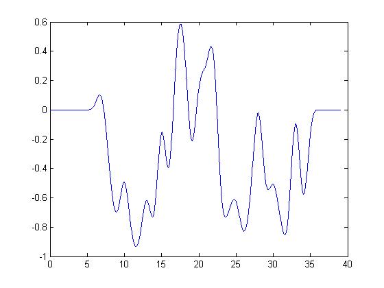
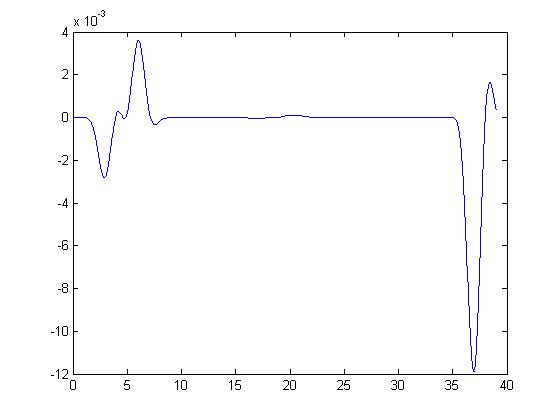
Figure 1: Plotted on the left is a nonseparable cubic spline signal $f$ with $K_{-}(f)=5,K_{+}(f)=32$ and $c(k),k\in{\mathbb{Z}}$, in (V.3). On the right is the difference between the above signal $f$ and the signal $f_{\varepsilon,L}$ reconstructed by the MEPS algorithm from the noisy samples (V.2) with $\varepsilon=10^{-7}$ and $L=7$. It is observed that the MEPS algorithm has higher accuracy to recover a signal inside its support.

Define a maximal reconstruction error of the MEPS algorithm by

$$e(\varepsilon,L):=\min_{\delta\in\{-1,1\}}\max_{k\in{\mathbb{Z}}}|c_{\varepsilon,L}(k)-\delta c(k)|.$$ (V.5)

As the cubic B-spline $B_{4}$ is a nonnegative function satisfying

$$\sum_{k\in{\mathbb{Z}}}B_{4}(t-k)=1\ {\rm for\ all}\ t\in{\mathbb{R}},$$

we have

$$\min_{\delta\in\{-1,1\}}\max_{t\in{\mathbb{R}}}|f_{\varepsilon,L}(t)-\delta f(t)|\leq e(\varepsilon,L).$$

For large odd integers $L$, the MEPS algorithm may not yield an approximation to the original signal in a noisy environment, as in Theorem IV.1 the stability requirement (IV.29) on the noise level $\varepsilon$ has exponential decay about $L\geq 1$. Our numerical simulations show that for large odd $L$, the MEPS algorithm may fail to save phases of nonseparable cubic spline signals, but its success rate to save phases (and then to reconstruct signals approximately) is still high for large $L$. Presented in Table I is the success rate after 500 trials for different noisy levels $\varepsilon$ and extension lengths $L$ to recover cubic spline signals $f$ in (V.1) with $c(k),k\in{\mathbb{Z}}$, in (V.3) and noisy samples in (V.2). Here the MEPS algorithm is considered to save the phase successfully if

$$e(\varepsilon,L)<0.1.$$ (V.6)

TABLE I: Success rate for different noisy levels $\varepsilon$ and extension lengths $L$.

	7	11	15	23	31	47
$10^{-5}$	$0.3140$	$0.2400$	$0.1180$	$0.0500$	0.0180	$0.0040$
$10^{-6}$	$0.8440$	$0.7780$	0.7360	0.5980	0.5200	$0.4220$
$10^{-7}$	$0.9840$	$0.9760$	0.9660	0.9480	0.9340	$0.9020$
$10^{-8}$	$0.9980$	$0.9960$	1	0.9980	$0.9860$	0.9980
$\leq 10^{-9}$	$1$	$1$	1	1	1	1

In the simulation, a successful recovery implies that $c_{\epsilon,L}(k)$ and $c(k),K_{-}(f)\leq k\leq K_{+}(f)$, have same signs,

$$c_{\varepsilon,L}(k)c(k)>0\ {\rm for\ all}\ K_{-}(f)\leq k\leq K_{+}(f).$$

The threshold selected in (V.6) for the maximal reconstruction error $e(\varepsilon,L)$ is less than

$$\min_{K_{-}(f)\leq k\leq K_{+}(f)-N+2}\Big{(}\frac{1}{N-1}\sum_{l=0}^{N-2}|c(k+l)|^{2}\Big{)}^{1/2},$$

which is similar to the quantity $S_{f}$ in (II.9) to measure the distance of a nonseparable signal $f$ to the set of all separable signals in a shift-invariant space, cf. Theorem II.6.

By (IV.11), (– ‣ (iii)) and Theorem IV.1, the maximal reconstruction error $e(\varepsilon,L)$ in (V.5) and the reconstruction errors $|c_{\varepsilon,L}(k)-c(k)|,k\not\in[K_{-}(f),K_{+}(f)]$, outside the support region are about the order $\sqrt{\varepsilon}$. Numerical simulations indicate that the reconstruction errors $|c_{\varepsilon,L}(k)-c(k)|,K_{-}(f)+N\leq k\leq K_{+}(f)-N$, are about the order $\varepsilon$, which is much smaller than the maximal reconstruction error $e(\varepsilon,L)$, see Figure 2.

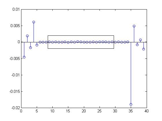
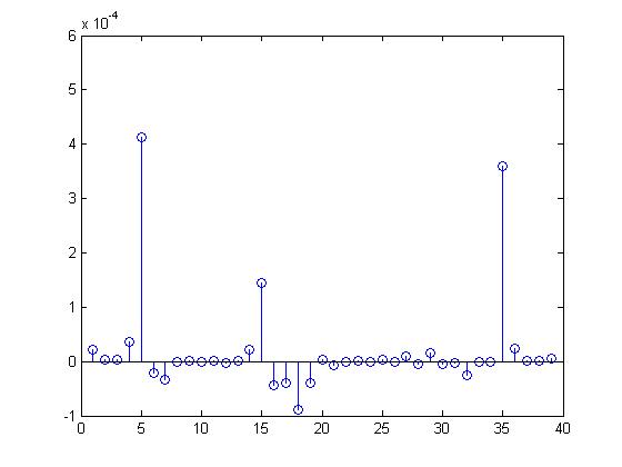
Figure 2: Plotted on the left is the difference $c_{\varepsilon,L}(k)-c(k),1\leq k\leq 39,$ between the reconstructed amplitudes and original amplitudes in Figure 1, while on the right is the squared difference $(c_{\varepsilon,L}(k))^{2}-(c(k))^{2},1\leq k\leq 39$. In the simulation, the maximal reconstruction error $e(\varepsilon,L)$ is $0.0190$, the maximal squared reconstruction error $e_{2}(\varepsilon,L)$ in (V.7) is $4.1204\times 10^{-4}$, and the maximal reconstruction error $\max_{K_{-}(f)+N\leq k\leq K_{+}(f)-N}|c_{\varepsilon,L}(k)-c(k)|$ inside the box is $1.5041\times 10^{-4}$. The maximal squared reconstructed error and the maximal reconstructed error inside the box are at the same order of $\|(\boldsymbol{\Phi}_{N})^{-1}\|\epsilon\approx 1.2390\times 10^{-4}$, cf. (IV.30).

An alternative to measure the phase retrieval error is the following maximal squared reconstructed error,

$$e_{2}(\varepsilon,L):=\max_{k\in{\mathbb{Z}}}|(c_{\varepsilon,L}(k))^{2}-(c(k))^{2}|.$$ (V.7)

For small $\varepsilon>0$, it follows from Theorem IV.1 that

$$e_{2}(\varepsilon,L)\leq 3e(\varepsilon,L)\big{(}\max_{k\in{\mathbb{Z}}}|c(k)|\big{)}\leq C\big{(}\max_{k\in{\mathbb{Z}}}|c(k)|\big{)}\sqrt{\varepsilon},$$

where $C$ is a positive constant. The above upper bound estimate for the measurement $e_{2}(\varepsilon,L)$ should not be optimal, as our numerical simulations indicate that the above alternative measurement $e_{2}(\varepsilon,L)$ is about the order $\varepsilon$, see Figure 2.

The success rate of the MEPS algorithm could have significant improvement if the phaseless samples $|f(y)|,y\in Y_{L}\cap[K_{-}(f),K_{+}(f)]$, of the original signal $f$ in (V.1) are a distance away from the origin. Such a requirement holds if the cubic spline signal $f$ has only “one” phase, i.e., $c(k)>0$ for all $K_{-}(f)\leq k\leq K_{+}(f)$. Presented in Table II is the success rate of the MEPS algorithm to recover the positive phase of nonseparable cubic spline signals $f$ in (V.1) with

$$c(k)\in[0.1,1]\ {\rm for\ all}\ K_{-}(f)\leq k\leq K_{+}(f)$$ (V.8)

after 500 trails, where the noise level $\varepsilon$, the extension length $L$ and the success threshold are the same as in Table I.

TABLE II: Success rate to recover cubic spline signals with “one” phase

	7	11	15	23	31	47
$10^{-4}$	0.6640	$0.6300$	0.5740	0.5420	0.5000	0.4040
$5*10^{-5}$	0.8840	$0.9080$	0.8600	0.8600	0.8540	0.8520
$\leq 10^{-5}$	1	$1$	1	1	1	1

Under the “one” phase assumption on the original signal, the extension parts (ii) and (iii) in the MEPS algorithm does not propagate noises at each extension step, because for all $1\leq l\leq(L-1)/2$, signs of $\tilde{z}_{\epsilon}(k^{\prime}L+l+\gamma_{n})$ in (IV.15) are the same as $f(k^{\prime}L+l+\gamma_{n}),1\leq l\leq(L-1)/2$, and similarly for $1\leq l^{\prime}\leq(L-1)/2$, signs of $\tilde{z}_{\epsilon}(k^{\prime}L-l^{\prime}+\gamma_{n}^{*})$ in (IV.20) are the same as $f(k^{\prime}L-l+\gamma_{n}^{*}),1\leq n\leq N$.

VI Conclusions

Let ${\mathcal{S}}(\phi)$ be the set of all real-valued signals in a shift-invariant space $V(\phi)$ that can, up to a sign, be reconstructed from its magnitude on the whole line. For a compactly supported continuous generator $\phi$, ${\mathcal{S}}(\phi)$ is neither the whole linear space $V(\phi)$ nor its convex subset. This is a different phenomenon from the bandlimited case, for which it is observed that all bandlimited signals can, up to a sign, be reconstructed from its magnitude on the whole line ([19, 24]).

Phase retrieval of signals in a shift-invariant space is a sampling and reconstruction problem. The set ${\mathcal{S}}(\phi)$ contains all nonseparable signals, which could be determined from its phaseless sampling on some sets with sampling rate large than the support length of the generator $\phi$.

Many algorithms have been introduced to solve a phase retrieval problem in the finite-dimensional setting. The MEPS algorithm is proposed to solve the infinite-dimensional phase retrieval problem for nonseparable signals in a shift-invariant space. The MEPS algorithm can be implemented in a distributed manner ([46, 47]), and it is stable against bounded sampling noises.

Appendix A Proof of Theorem II.2

($\Longrightarrow$)  Suppose, on the contrary, that there exist nonzero signals $f_{1},f_{2}\in V$ such that $f=f_{1}+f_{2}$ and $f_{1}f_{2}=0$. Set $g=f_{1}-f_{2}\in V$. Then $g\neq\pm f$ and $|g|=|f|=\sqrt{|f_{1}|^{2}+|f_{2}|^{2}}$. This is a contradiction.

($\Longleftarrow$)  Let $g$ be a signal in $V$ with $|g|=|f|$. Set $g_{1}:=(f+g)/2\in V$ and $g_{2}:=(f-g)/2\in V$. Then $f=g_{1}+g_{2}$ and $g_{1}g_{2}=0$. This together with nonseparability of the signal $f$ implies that either $g_{1}\equiv 0$ or $g_{2}\equiv 0$. Hence $g$ is either $-f$ or $f$. This completes the proof.

Appendix B Proof of Theorem II.6

We divide the proof into three implications iii)$\Longrightarrow$i), i)$\Longrightarrow$ii) and ii)$\Longrightarrow$iii).

iii)$\Longrightarrow$i):  The implication follows immediately from Theorem II.2.

i)$\Longrightarrow$ii):  Set $K_{\pm}=K_{\pm}(f)$. For $K_{-}+1-N<k<K_{-}+1$ or $K_{+}+1-N<k<K_{+}+1$, the conclusion $\sum_{l=0}^{N-2}|c(k+l)|^{2}\neq 0$ follows from the definitions of $K_{-}$ and $K_{+}$. Then it remains to establish the statement ii) for $K_{-}<k<K_{+}+2-N$. Suppose, on the contrary, that

$$\sum_{l=0}^{N-2}|c(k_{1}+l)|^{2}=0$$ (B.1)

for some $K_{-}<k_{1}<K_{+}-N+2$. Set

$$f_{1}(t):=\sum_{l=K_{-}}^{k_{1}-1}c(l)\phi(t-l)\ \ {\rm and}\ \ f_{2}(t):=\sum_{l=k_{1}+N-1}^{K_{+}}c(l)\phi(t-l).$$

Then

$$f=f_{1}+f_{2}\ \ {\rm and}\ \ f_{1}f_{2}=0$$ (B.2)

by (B.1) and the observation that $f_{1}$ and $f_{2}$ are supported in $(-\infty,k_{1}+N-1]$ and $[k_{1}+N-1,\infty)$ respectively. Clearly, $f_{1}$ and $f_{2}$ are nonzero signals in $V(\phi)$. This together with (B.2) implies that $f$ is separable, which contradicts to the assumption i).

ii)$\Longrightarrow$iii):  To prove the implication, we need a lemma.

Lemma B.1.

Let $\phi$ and $X$ be as in Theorem II.6. Then for any $l\in{\mathbb{Z}}$ and signal $g(t)=\sum_{k=-\infty}^{\infty}d(k)\phi(t-k)\in V(\phi)$, coefficients $d(k),l-N+1\leq k\leq l$, are completely determined, up to a sign, by phaseless samples $|g(x_{m}+l)|,\ x_{m}\in X$, of the signal $g$.

The above lemma follows immediately from [10, Theorem 2.8] and the observation that

$$g(x_{m}+l)=\sum_{k=l-N+1}^{l}d(k)\phi(x_{m}+l-k),\ \ x_{m}\in X.$$

Take a particular integer $K_{-}-1<k_{0}<K_{+}+1$ with $c(k_{0})\neq 0$. Without loss of generality, we assume that

$$c(k_{0})>0,$$ (B.3)

otherwise replacing $f$ by $-f$.

Using (B.3) and applying Lemma B.1 with $g$ and $l$ replaced by $f$ and $k_{0}$ respectively, we conclude that $c({k_{0}-N+1}),\cdots,c({k_{0}})$ are completely determined by phaseless samples $|f(X+k_{0})|$ of the signal $f$ on $X+k_{0}$. Now we prove that

$$c(k),\ k\leq k_{0},\ {\rm are\ determined\ by}\ |f(X+k)|,\ k\leq k_{0}$$ (B.4)

by induction. Inductively we assume that $c({k}),k_{0}-p-N+1\leq k\leq k_{0}$, are determined from $|f(X+k)|,k_{0}-p\leq k\leq k_{0}$. The inductive proof is complete if $k_{0}-p-N+1\leq K_{-}$. Otherwise $k_{0}-p-N+1>K_{-}$ and

$$\sum_{l=0}^{N-2}|c({k_{0}-p-N+l+1})|^{2}\neq 0$$ (B.5)

by the assumption ii). Applying Lemma B.1 with $g$ and $k_{0}$ replaced by $f$ and $k_{0}-p-1$ respectively, we conclude that $c({k_{0}-N-p}),\cdots,c({k_{0}-p-1})$ are determined by $|f(X+k_{0}-p-1)|$ up to a global phase. This together with (B.5) and the inductive hypothesis implies that $c({k_{0}-N-p}),\cdots,c({k_{0}-p-1})$ is determined by $|f(X+k)|,k_{0}-p-1\leq k\leq k_{0}$. Thus the inductive argument can proceed.

Using the similar argument, we can show that

$$c(k),\ k\geq k_{0},\ {\rm are\ determined\ by}\ |f(X+k)|,k\geq k_{0}.$$ (B.6)

Combining (B.4) and (B.6) completes the proof.

Appendix C Proof of Theorem III.1

By (III.1) it suffices to prove that

$$\#(I\cap[a,b])\geq b-a-N+1$$

for all integers $a$ and $b$ with $b-a\geq N$. Suppose, on the contrary, that

$$\#(I\cap[a_{0},b_{0}])<b_{0}-a_{0}-N+1$$ (C.1)

for some integers $a_{0}$ and $b_{0}$. Let

$${\mathcal{N}}=\Big{\{}f(t):=\sum_{k=a_{0}}^{b_{0}-N}c(k)\phi(t-k),\ f(y)=0\ {\rm for\ all}\ y\in I\Big{\}}.$$

Then ${\mathcal{N}}$ contains some nonzero signals in $V(\phi)$, because any signal of the form $\sum_{k=a_{0}}^{b_{0}-N}c(k)\phi(t-k)$ is supported in $[a_{0},b_{0}]$, and the homogenous linear system

$$\sum_{k=a_{0}}^{b_{0}-N}c(k)\phi(y-k)=0,\ \ y\in I\cap[a_{0},b_{0}]$$

of size $(\#(I\cap[a_{0},b_{0}]))\times(b_{0}-a_{0}-N+1)$ has a nontrivial solution by (C.1).

Take a nonzero signal $f\in{\mathcal{N}}$ with minimal support length. By the assumption on the set $I$, it must be separable as it is a nonzero signal having zero magnitude measurements on $I$. Therefore by Theorem II.6 there exist nonzero signals $f_{1}$ and $f_{2}\in V(\phi)$ and an integer $k_{0}\in(a_{0},b_{0})$ such that $f_{1}$ vanishes outside $[k_{0},b_{0}]$, $f_{2}$ vanishes outside $[a_{0},k_{0}]$ and $f=f_{1}+f_{2}$. This implies that both $f_{1}$ and $f_{2}$ are nonzero signals in ${\mathcal{N}}$, which contradicts to the assumption that $f\in{\mathcal{N}}$ has minimal support length.

Appendix D Proof of Theorem III.4

To prove Theorem III.4, we need a technical lemma.

Lemma D.1.

Let $\gamma_{n}$ and $\gamma_{n}^{\ast}$, $1\leq n\leq N$, and $\phi$ be as in Theorem III.4. Then

$$\left(\begin{array}[]{ccc}\phi(\gamma_{1})&\ldots&\phi(\gamma_{N})\\ \displaystyle{\sum_{l=0}^{N-2}}a(l)\phi(\gamma_{1}+l+1)&\ldots&\displaystyle{\sum_{l=0}^{N-2}}a(l)\phi(\gamma_{N}+l+1)\end{array}\right)$$ (D.1)

and

$$\left(\begin{array}[]{ccc}\phi(\gamma^{\ast}_{1}+N-1)&\ldots&\phi(\gamma^{\ast}_{N}+N-1)\\ \displaystyle{\sum_{l=0}^{N-2}}a(l)\phi(\gamma^{\ast}_{1}+l)&\ldots&\displaystyle{\sum_{l=0}^{N-2}}a(l)\phi(\gamma^{\ast}_{N}+l)\end{array}\right)$$ (D.2)

have rank $2$ for any nonzero vector $(a(0),\ldots,a(N-2))$.

Proof.

We prove (D.1) by indirect proof. Suppose, on the contrary, that

$$\frac{\sum_{l=0}^{N-2}a(l)\phi(\gamma_{n}+l+1)}{\phi(\gamma_{n})}=\alpha,\ \ 1\leq n\leq N$$

for some $\alpha\in{\mathbb{R}}$. This together with nonsingularity of the matrix $(\phi(\gamma_{n}+m))_{1\leq n\leq N,0\leq m\leq N-1}$ implies that $(-\alpha,a(0),\ldots,a({N-2}))$ is a zero vector, which is a contradiction.

The full rank property (D.2) can be proved similarly. ∎

Proof of Theorem III.4.

Due to the shift-invariance, without loss of generality, we assume that $k_{0}=0$. Set $K_{\pm}=K_{\pm}(f)$. We divide the proof into three cases: $K_{-}\leq 0\leq K_{+}+N-1$, $K_{-}\geq 1$ and $K_{+}\leq-N$.

Case 1: $K_{-}\leq 0\leq K_{+}+N-1$.

In this case, it follows from Theorem II.6 and nonseparability of the signal $f$ that there exists $-N+2\leq n_{0}\leq 0$ such that $c({l_{0}})\neq 0$ and $c(l)=0$ for all $l_{0}<l\leq 0$. Without loss of generality, we assume that

$$c({l_{0}})>0\ {\ \rm and\ }\ c(l)=0\ {\ \rm for\ all\ }\ l_{0}<l\leq 0,$$ (D.3)

otherwise replacing $f$ by $-f$. By (D.3) and Lemma B.1,

$$c({-N+1}),\ldots,c(-1),c(0)$$ (D.4)

are determined from phaseless samples $|f(X)|$. Next we prove by induction that $c(k),k\geq-N+1$, are determined by phaseless samples $|f(X)|$ and $|f(\Gamma+q)|,q\geq 1$. Inductively, we assume that $c(k),-N+1\leq k<p$, can be recovered from $|f(X)|$ and $|f(\Gamma+q)|,1\leq q<p$. The induction proof is finished if $p>K_{+}$. Now it remains to consider $p\leq K_{+}$.

Observe that

$$f(\gamma_{n}+p) \hskip-5.78172pt= \hskip-5.78172ptc(p)\phi(\gamma_{n})+\sum_{l=0}^{N-2}c({p-l-1})\phi(\gamma_{n}+l+1)$$ (D.5)

$$\hskip-5.78172pt=: \hskip-5.78172ptc(p)\phi(\gamma_{n})+\alpha(n)\ \ {\rm for\ all}\ \gamma_{n}\in\Gamma.$$

Taking squares at both sides of the above equations yields

$$|\phi(\gamma_{n})|^{2}(c(p))^{2}+2\phi(\gamma_{n})\alpha(n)c(p)+|\alpha(n)|^{2}=|f(\gamma_{n}+p)|^{2},$$

where $1\leq n\leq N$. Moving $|\alpha(n)|^{2}$ to the right hand side and then dividing $\phi(\gamma_{n})$ at both sides, we obtain

$$\phi(\gamma_{n})(c(p))^{2}+2\alpha(n)c(p)=\frac{|f(\gamma_{n}+p)|^{2}-|\alpha(n)|^{2}}{\phi(\gamma_{n})},$$ (D.6)

where $1\leq n\leq N$. As $K_{-}<p\leq K_{+}$, we obtain from Theorem II.6 that $(c({p-N+1}),\ldots,c({p-1}))$ is a nonzero vector. Therefore by Lemma D.1, the $2\times N$ matrix

$$\left(\begin{array}[]{ccc}\phi(\gamma_{1})&\cdots&\phi(\gamma_{N})\\ \alpha(1)&\ldots&\alpha(N)\end{array}\right)$$

has rank $2$. So there is a unique solution

$$c(p)=\frac{h_{2}({\boldsymbol{\alpha}},{\boldsymbol{\eta}})}{2h_{1}({\boldsymbol{\alpha}})}$$ (D.7)

to the linear system (D.6), where $h_{1},h_{2}$ are functions given in (IV.2) and (IV.4) respectively, ${\boldsymbol{\alpha}}=(\alpha(1),\ldots,\alpha(N))$, and

$${\boldsymbol{\eta}}=(|f(\gamma_{1}+p)|^{2}-|\alpha(1)|^{2},\ldots,|f(\gamma_{N}+p)|^{2}-|\alpha(N)|^{2}).$$

This completes the inductive proof. Hence $c(k),k\geq-N+1$, are determined from $|f(X)|$ and $|f(\Gamma+q)|,q\geq 1$.

Finally we use similar arguments to determine $c(k),k\leq-N+1$, from $|f(X)|$ and $|f(\Gamma^{\ast}+q)|,q\leq-1$. Inductively, we assume that $c(k),\tilde{p}<k\leq 0$, has been recovered from $|f(X)|$ and $|f(\Gamma^{\ast}+q)|,\tilde{p}+N-1<q\leq-1$. The induction proof is done if $\tilde{p}<K_{-}$. Then it remains to discuss $\tilde{p}\geq K_{-}$. Observe that

$$f(\gamma^{\ast\ast}_{n}+\tilde{p}) \hskip-7.22743pt= \hskip-7.22743ptc({\tilde{p}})\phi(\gamma^{\ast\ast}_{n})+\sum_{l=0}^{N-2}c(\tilde{p}+N-1-l)\phi(\gamma^{*}_{n}+l)$$ (D.8)

$$\hskip-7.22743pt=: \hskip-7.22743ptc({\tilde{p}})\phi(\gamma_{n}^{\ast\ast})+\alpha^{\ast}(n).$$

where $\gamma_{n}^{\ast\ast}=\gamma^{\ast}_{n}+N-1,1\leq n\leq N$. By Lemma D.1, the $2\times N$ matrix

$$\left(\begin{array}[]{ccc}\phi(\gamma_{1}^{\ast\ast})&\ldots&\phi(\gamma^{\ast\ast}_{N})\\ \alpha^{\ast}(1)&\ldots&\alpha^{\ast}(N)\end{array}\right)$$

has rank $2$. Therefore

$$c_{\tilde{p}}=\frac{h_{2}^{*}({\boldsymbol{\alpha}}^{*},{\boldsymbol{\eta}}^{*})}{2h_{1}^{*}({\boldsymbol{\alpha}}^{*})},$$ (D.9)

where $h_{1}^{*}$ and $h_{2}^{*}$ are given in (IV.3) and (IV.5) respectively, ${\boldsymbol{\alpha}}^{\ast}=(\alpha^{\ast}(1),\ldots,\alpha^{\ast}(N))$, and

$${\boldsymbol{\eta}}^{\ast}=(|f(\gamma_{1}^{\ast\ast}+\tilde{p})|^{2}-|\alpha^{\ast}(1)|^{2},\ldots,|f(\gamma_{N}^{\ast\ast}+\tilde{p})|^{2}-|\alpha^{\ast}(N)|^{2}).$$

This completes the inductive proof. Therefore $c(k),k\leq 0$, are determined from $|f(X)|$ and $|f(\Gamma^{\ast}+q)|,q\leq-1$.

Case 2: $K_{-}\geq 1$.

In this case, the signal $f$ is supported in $[1,\infty)$. Without loss of generality, we assume that $c({K_{-}})>0$, otherwise considering $-f$ instead of $f$. From the definition of $K_{-}$ and the supporting property of $\phi$, we have

$$f(\gamma_{n}+K_{-})=c({K_{-}})\phi(\gamma_{n}),\ \ \gamma_{n}\in\Gamma.$$

Thus

$$c(K_{-})=\frac{\sum_{n=1}^{N}|\phi(\gamma_{n})||f(\gamma_{n}+K_{-})|}{\sum_{n=1}^{N}|\phi(\gamma_{n})|^{2}}.$$

Then following the same procedure as in Case 1, we obtain that $c(k),k\geq K_{-}$, are determined from $|f(\Gamma+q)|,q\geq K_{-}$.

Case 3: $K_{+}\leq-N$.

In this case, the signal $f$ is supported in $(-\infty,0]$, and $c({K_{+}})$ can be obtained, up to a sign, from phaseless samples $|f(\Gamma^{\ast}+K_{+}+N-1)|$. Following the same procedure as in Case 1, we can determine $c(k),k\leq K_{+}\leq-N$, from $|f(\Gamma^{\ast}+q)|,q\leq K_{+}+N-1$. ∎

Appendix E Proof of Theorem IV.1

The proof of Theorem IV.1 is quite technical. It includes three propositions on the approximation property of vectors in the first three steps of the MEPS algorithm (IV.8)–(IV.25), and one proposition on the phase adjustment.

To prove Theorem IV.1, we first show that for any $k^{\prime}\in{\mathbb{Z}}$, the vector ${\bf c}_{\boldsymbol{\epsilon},k^{\prime}}^{0}$ in the first step of the MEPS algorithm approximates, up to a sign, the original vector ${\bf c}$ on $[k^{\prime}L+1-N,k^{\prime}L]$.

Proposition E.1.

Let ${\bf c},{\boldsymbol{\epsilon}}$ be as in Theorem IV.1, and ${\bf c}_{\boldsymbol{\epsilon},k^{\prime}}^{0}$, $k^{\prime}\in{\mathbb{Z}}$, be as in (IV.8). Then for any $k^{\prime}\in{\mathbb{Z}}$, there exists $\delta_{k^{\prime}}\in\{-1,1\}$ such that

$$\sum_{k=k^{\prime}L-N+1}^{k^{\prime}L}|c_{\boldsymbol{\epsilon},k^{\prime}}^{0}(k)-\delta_{k^{\prime}}c(k)|^{2}\leq 8N\|(\Phi_{N})^{-1}\|^{2}|{\boldsymbol{\epsilon}}|.$$ (E.1)

Proof.

Set $x_{m,k^{\prime}}=x_{m}+k^{\prime}L,1\leq m\leq 2N-1$. Then

$$\hskip-5.78172pt\sum_{m=1}^{2N-1}\Big{(}\Big{|}\sum_{k=k^{\prime}L-N+1}^{k^{\prime}L}c_{\boldsymbol{\epsilon},k^{\prime}}^{0}(k)\phi(x_{m,k^{\prime}}-k)\Big{|}$$

$$\hskip-5.78172pt\qquad\qquad-\Big{|}\sum_{k=k^{\prime}L-N+1}^{k^{\prime}L}c(k)\phi(x_{m,k^{\prime}}-k)\Big{|}\Big{)}^{2}$$

$$\hskip-5.78172pt\leq \hskip-5.78172pt2\sum_{m=1}^{2N-1}\Bigg{(}\Big{|}\sum_{k=k^{\prime}L-N+1}^{k^{\prime}L}c_{\boldsymbol{\epsilon},k^{\prime}}^{0}(k)\phi(x_{m,k^{\prime}}-k)\Big{|}$$

$$\hskip-5.78172pt\quad-\sqrt{z_{\boldsymbol{\epsilon}}(x_{m,k^{\prime}})}\Bigg{)}^{2}+2\sum_{m=0}^{2N-1}\Bigg{(}\sqrt{z_{\boldsymbol{\epsilon}}(x_{m,k^{\prime}})}$$

$$\hskip-5.78172pt\qquad\qquad-\Big{|}\sum_{k=k^{\prime}L-N+1}^{k^{\prime}L}c(k)\phi(x_{m,k^{\prime}}-k)\Big{|}\Bigg{)}^{2}$$

$$\hskip-5.78172pt\leq \hskip-5.78172pt4\sum_{m=1}^{2N-1}\Big{|}|f(x_{m,k^{\prime}})|-\sqrt{z_{\boldsymbol{\epsilon}}(x_{m,k^{\prime}})}\Big{|}^{2}$$

$$\hskip-5.78172pt\leq \hskip-5.78172pt4\sum_{m=1}^{2N-1}|\boldsymbol{\epsilon}(x_{m,k^{\prime}})|\leq 8N|{\boldsymbol{\epsilon}}|,$$

where the second inequality holds by (IV.9), and the third estimate follows from the triangle inequality

$$|\sqrt{x^{2}+y}-|x||\leq\sqrt{|y|}$$ (E.2)

for all $x\geq 0$ and $y\geq-x^{2}$. Therefore there exist $1\leq m_{1},\ldots,m_{N}\leq 2N-1$ and $\delta_{k^{\prime}}\in\{-1,1\}$ such that

$$\sum_{l=1}^{N}\Big{(}\sum_{k=k^{\prime}L-N+1}^{k^{\prime}L}\big{(}c_{\boldsymbol{\epsilon},k^{\prime}}^{0}(k)-\delta_{k^{\prime}}c(k)\big{)}\phi(x_{m_{l},k^{\prime}}-k)\Big{)}^{2}\leq 8N|{\boldsymbol{\epsilon}}|.$$

This proves (E.1). ∎

To prove Theorem IV.1, we next verify that for any $k^{\prime}\in{\mathbb{Z}}$, the vector ${\bf c}_{\boldsymbol{\epsilon},k^{\prime}}^{1/2}$ in the second step of the MEPS algorithm is, up to a sign, not far away from ${\bf c}$ on $[k^{\prime}L+1-N,k^{\prime}L+(L-1)/2]$.

Proposition E.2.

Let ${\bf c},{\boldsymbol{\epsilon}}$ be as in Theorem IV.1, and let vectors ${\bf c}_{\boldsymbol{\epsilon},k^{\prime}}^{1/2},k^{\prime}\in{\mathbb{Z}}$, be as in (IV.16). Then for any $k^{\prime}\in{\mathbb{Z}}$, there exists $\delta_{k^{\prime}}\in\{-1,1\}$ such that

$$|c^{1/2}_{\boldsymbol{\epsilon},k^{\prime}}(k)-\delta_{k^{\prime}}c(k)|\leq\|(\Phi_{N})^{-1}\|(C_{f,\phi})^{k-k^{\prime}L+N-1}\sqrt{8N|\boldsymbol{\epsilon}|}$$ (E.3)

for all $k^{\prime}L+1-N\leq k\leq k^{\prime}L+(L-1)/2$.

To prove Proposition E.2, we need a technical lemma.

Lemma E.3.

Let $h_{2}$ and $h_{2}^{\ast}$ be as in (IV.4) and (IV.5). Then

$$|h_{2}({\bf e}_{1},{\bf e}_{2})|\leq\frac{\|{\bf e}_{1}\|\|{\bf e}_{2}\|}{\min_{1\leq n\leq N}|\phi(\gamma_{n})|}$$ (E.4)

and

$$|h_{2}^{\ast}({\bf e}_{1},{\bf e}_{2})|\leq\frac{\|{\bf e}_{1}\|\|{\bf e}_{2}\|}{\min_{1\leq n\leq N}|\phi(\gamma_{n}^{*}+N-1)|}$$ (E.5)

for all ${\bf e}_{1},{\bf e}_{2}\in{\mathbb{R}}^{N}$.

Proof.

The upper bound estimate (E.4) holds, since

$$|h_{2}({\bf e}_{1},{\bf e}_{2})|\hskip-3.61371pt \hskip-3.61371pt= \hskip-7.22743pt\Big{|}\sum_{n=1}^{N}\Big{(}\frac{e_{2}(n)}{\phi(\gamma_{n})}-\alpha\phi(\gamma_{n})\Big{)}e_{1}(n)\Big{|}$$

$$\hskip-3.61371pt\leq \hskip-7.22743pt\Big{(}\sum_{n=1}^{N}\Big{|}\frac{e_{2}(n)}{\phi(\gamma_{n})}-\alpha\phi(\gamma_{n})\Big{|}^{2}\Big{)}^{1/2}\|{\bf e}_{1}\|$$

$$\hskip-3.61371pt= \hskip-7.22743pt\Big{(}\sum_{n=1}^{N}\Big{|}\frac{e_{2}(n)}{\phi(\gamma_{n})}\Big{|}^{2}-\alpha^{2}\sum_{n=1}^{N}|\phi(\gamma_{n})|^{2}\Big{)}^{1/2}\|{\bf e}_{1}\|$$

$$\hskip-3.61371pt\leq \hskip-7.22743pt\Big{(}\sum_{n=1}^{N}\Big{|}\frac{e_{2}(n)}{\phi(\gamma_{n})}\Big{|}^{2}\Big{)}^{1/2}\|{\bf e}_{1}\|,$$

where $\alpha=\frac{\sum_{n=1}^{N}e_{2}(n)}{\sum_{n=1}^{N}|\phi(\gamma_{n})|^{2}}$.

Applying similar argument, we can prove (E.5). ∎

Now we return to the proof of Proposition E.2.

Proof of Proposition E.2.

Take $k^{\prime}\in{\mathbb{Z}}$, and let ${\bf c}_{\boldsymbol{\epsilon},k^{\prime},l}^{1/2},0\leq l\leq(L-1)/2$, be as in (IV.11)–(IV.15). Observe that

$$c^{1/2}_{\boldsymbol{\epsilon},k^{\prime}}(k)=c^{1/2}_{\boldsymbol{\epsilon},k^{\prime},l}(k)$$

for all $k\in[k^{\prime}L+1-N,k^{\prime}L+(L-1)/2]$ and $l\geq\min(k-k^{\prime}L+N-1,(L-1)/2)$. Then it suffices to find $\delta_{k^{\prime}}\in\{-1,1\}$ such that

$$\hskip-5.78172pt\sum_{k=k^{\prime}L+l+1-N}^{k^{\prime}L+l}|c^{1/2}_{\boldsymbol{\epsilon},k^{\prime},l}(k)-\delta_{k^{\prime}}c(k)|^{2}$$

$$\hskip 5.78172pt\qquad\leq 8N\|(\Phi_{N})^{-1}\|^{2}(C_{f,\phi})^{2l}|\boldsymbol{\epsilon}|\$$ (E.6)

for all $0\leq l\leq(L-1)/2$.

We establish the above conclusion (E) by induction. The conclusion (E) for $l=0$ follows from (E.1) in Proposition E.1. Inductively we assume that

$$\hskip-5.78172pt\sum_{k=k^{\prime}L+l_{0}+1-N}^{k^{\prime}L+l_{0}}|c^{1/2}_{\boldsymbol{\epsilon},k^{\prime},l_{0}}(k)-\delta_{k^{\prime}}c(k)|^{2}$$

$$\hskip 5.78172pt\qquad\leq 8N\|(\Phi_{N})^{-1}\|^{2}(C_{f,\phi})^{2l_{0}}|\boldsymbol{\epsilon}|$$ (E.7)

for some $0\leq l_{0}\leq(L-1)/2$. Set ${\bf e}_{\boldsymbol{\epsilon},1}=(\alpha_{\boldsymbol{\epsilon}}(1),\ldots,\alpha_{\boldsymbol{\epsilon}}(N))$ and ${\bf e}_{0,1}=(\alpha(1),\ldots,\alpha(N))$, where

$$\alpha_{\boldsymbol{\epsilon}}(n)=\sum_{l^{\prime}=0}^{N-2}c^{1/2}_{\boldsymbol{\epsilon},k^{\prime},l_{0}}(k^{\prime}L+l_{0}-l^{\prime})\phi(\gamma_{n}+l^{\prime}+1)$$

and

$$\alpha(n)=\sum_{l^{\prime}=0}^{N-2}c(k^{\prime}L+l_{0}-l^{\prime})\phi(\gamma_{n}+l^{\prime}+1),1\leq n\leq N.$$

Now we divide into two cases to prove (E) for $l=l_{0}+1\leq(L-1)/2$.

Case 1: $\sum_{k=k^{\prime}L+l_{0}+2-N}^{k^{\prime}L+l_{0}}|c(k)|^{2}=0$.

Set

$$\alpha_{\boldsymbol{\epsilon}}(0)=\frac{\sum_{n=1}^{N}\phi(\gamma_{n})\alpha_{\boldsymbol{\epsilon}}(n)}{\sum_{n=1}^{N}|\phi(\gamma_{n})|^{2}}\ \ {\rm and}\ \ \alpha(0)=\frac{\sum_{n=1}^{N}\phi(\gamma_{n})\alpha(n)}{\sum_{n=1}^{N}|\phi(\gamma_{n})|^{2}}.$$

Therefore for the function $h_{1}$ in (IV.2), we have

$$\hskip-9.39545pth_{1}({\bf e}_{\boldsymbol{\epsilon},1}) \hskip-7.22743pt= \hskip-5.78172pt\sum_{n=1}^{N}(\alpha_{\boldsymbol{\epsilon}}(n)-\phi(\gamma_{n})\alpha_{\boldsymbol{\epsilon}}(0))^{2}$$ (E.8)

$$\hskip-5.78172pt\leq \hskip-5.78172pt\sum_{n=1}^{N}|\alpha_{\boldsymbol{\epsilon}}(n)|^{2}\leq\|\Phi\|^{2}\sum_{k=k^{\prime}L+l_{0}+2-N}^{k^{\prime}L+l_{0}}|c^{1/2}_{\boldsymbol{\epsilon},k^{\prime},l_{0}}(k)|^{2}$$

$$\hskip-5.78172pt\leq \hskip-5.78172pt8N\|\Phi\|^{2}\|(\Phi_{N})^{-1}\|^{2}(C_{f,\phi})^{2l_{0}}|\boldsymbol{\epsilon}|$$

$$\hskip-5.78172pt\leq \hskip-5.78172pt\frac{\|\Phi\|^{2}S_{f}}{2^{4}N^{2}(C_{f,\phi})^{4N+L-5-2l_{0}}}\leq M_{0},$$

where the third inequality follows from the inductive hypothesis (E) and the last two estimates hold by (IV.28) and (IV.29). Hence

$$c^{1/2}_{\boldsymbol{\epsilon},k^{\prime},l_{0}+1}(l_{0}^{*}+1)=\frac{\sum_{n=1}^{N}|\phi(\gamma_{n})|\sqrt{z_{\boldsymbol{\epsilon}}(\gamma_{n}+l_{0}^{*}+1)}}{\sum_{n=1}^{N}|\phi(\gamma_{n})|^{2}}$$ (E.9)

by (IV.11), where $\ell_{0}^{*}=k^{\prime}L+l_{0}$.

Case 1a: $c(k^{\prime}L+l_{0}+1)=0$.

In this subcase,

$$z_{\boldsymbol{\epsilon}}(\gamma_{n}+k^{\prime}L+l_{0}+1)=\boldsymbol{\epsilon}(\gamma_{n}+k^{\prime}L+l_{0}+1),1\leq n\leq N,$$

and

$$\hskip-5.78172pt|c^{1/2}_{\boldsymbol{\epsilon},k^{\prime},l_{0}+1}(k^{\prime}L+l_{0}+1)-\delta_{k^{\prime}}c(k^{\prime}L+l_{0}+1)|$$ (E.10)

$$\hskip-5.78172pt= \hskip-5.78172pt\frac{\sum_{n=1}^{N}|\phi(\gamma_{n})|\sqrt{\boldsymbol{\epsilon}(\gamma_{n}+k^{\prime}L+l_{0}+1)}}{\sum_{n=1}^{N}|\phi(\gamma_{n})|^{2}}$$

$$\hskip-5.78172pt\leq \hskip-5.78172pt\Big{(}\sum_{n=1}^{N}|\phi(\gamma_{n})|^{2}\Big{)}^{-1/2}\hskip-5.78172pt\sqrt{N|{\boldsymbol{\epsilon}}|}$$

$$\hskip-5.78172pt\leq \hskip-5.78172pt\|(\Phi_{N})^{-1}\|\sqrt{N|{\boldsymbol{\epsilon}}|}.$$

Case 1b: $c(k^{\prime}L+l_{0}+1)\neq 0$.

In this subcase, it follows from Theorem II.6 that

$$c(k)=0\ {\rm for\ all}\ k\leq k^{\prime}L+l_{0}.$$

Therefore the inductive hypothesis (E) holds for all $0\leq l\leq l_{0}$ with arbitrary $\delta_{k^{\prime}}\in\{-1,1\}$. So we may select

$$\delta_{k^{\prime}}=\frac{c(k^{\prime}L+l_{0}+1)}{|c(k^{\prime}L+l_{0}+1)|}$$

in this subcase. Hence

$$\hskip-5.78172pt|c^{1/2}_{\boldsymbol{\epsilon},k^{\prime},l_{0}+1}(k^{\prime}L+l_{0}+1)-\delta_{k^{\prime}}c(k^{\prime}L+l_{0}+1)|$$ (E.11)

$$\hskip-5.78172pt\leq \hskip-5.78172pt\frac{\sum_{n=1}^{N}|\phi(\gamma_{n})|\sqrt{|\boldsymbol{\epsilon}(\gamma_{n}+k^{\prime}L+l_{0}+1)|}}{\sum_{n=1}^{N}|\phi(\gamma_{n})|^{2}}$$

$$\hskip-5.78172pt\leq \hskip-5.78172pt\Big{(}\sum_{n=1}^{N}|\phi(\gamma_{n})|^{2}\Big{)}^{-1/2}\hskip-5.78172pt\sqrt{N|{\boldsymbol{\epsilon}}|}\leq\|(\Phi_{N})^{-1}\|\sqrt{N|{\boldsymbol{\epsilon}}|},$$

where the first equality follows from (E.2), (E.9) and

$$f(\gamma_{n}+k^{\prime}L+l_{0}+1)=c(k^{\prime}L+l_{0}+1)\phi(\gamma_{n}),1\leq n\leq N.$$

Thus for the Case 1, the estimates in (E.10) and (E.11), together with the inductive hypothesis (E), imply (E) for $l=l_{0}+1$.

Case 2: $\sum_{k=k^{\prime}L+l_{0}+2-N}^{k^{\prime}L+l_{0}}|c(k)|^{2}\neq 0$.

In this case,

$$\|{\bf e}_{\boldsymbol{\epsilon},1}-\delta_{k^{\prime}}{\bf e}_{\boldsymbol{0},1}\|\leq\|\Phi\|\|(\Phi_{N})^{-1}\|(C_{f,\phi})^{l_{0}}\sqrt{8N|{\boldsymbol{\epsilon}}|}$$ (E.12)

by inductive hypothesis (E), and

$$\|{\bf e}_{\boldsymbol{\epsilon},1}\| \hskip-5.78172pt\leq \hskip-5.78172pt\|{\bf e}_{\boldsymbol{\epsilon},1}-\delta_{k^{\prime}}{\bf e}_{\boldsymbol{0},1}\|+\|{\bf e}_{\boldsymbol{0},1}\|$$ (E.13)

$$\hskip-5.78172pt\leq \hskip-5.78172pt2\|\Phi\|\Big{(}\sum_{k=k^{\prime}L+l_{0}+2-N}^{k^{\prime}L+l_{0}}|c(k)|^{2}\Big{)}^{1/2}$$

by (IV.29) and the property that

$$\|\Phi\|\|(\Phi_{N})^{-1}\|\geq 1.$$ (E.14)

Therefore

$$\hskip-23.84923pth_{1}({\bf e}_{\boldsymbol{\epsilon},1}) \hskip-7.22743pt= \hskip-5.78172pt\sum_{n=1}^{N}(\alpha_{\boldsymbol{\epsilon}}(n)-\phi(\gamma_{n})\alpha_{\boldsymbol{\epsilon}}(0))^{2}$$ (E.15)

$$\hskip-7.22743pt\geq \hskip-5.78172pt\|(\Phi_{N})^{-1}\|^{-2}\hskip-5.78172pt\sum_{k=k^{\prime}L+l_{0}+2-N}^{k^{\prime}L+l_{0}}|c^{1/2}_{\boldsymbol{\epsilon},k^{\prime}}(k)|^{2}$$

$$\hskip-7.22743pt\geq \hskip-5.78172pt\frac{\sum_{k=k^{\prime}L+l_{0}+2-N}^{k^{\prime}L+l_{0}}|c(k)|^{2}}{4\|(\Phi_{N})^{-1}\|^{2}}>M_{0},$$

where the second inequality follows from (IV.29) and the inductive hypothesis (E), and the last inequality holds by (II.9) and (IV.28). Hence

$$d_{\boldsymbol{\epsilon},k^{\prime}}(k^{\prime}L+l_{0}+1)=\frac{h_{2}({\bf e}_{\boldsymbol{\epsilon},1},{\bf e}_{\boldsymbol{\epsilon},2})}{2h_{1}({\bf e}_{\boldsymbol{\epsilon},1})}$$ (E.16)

by (IV.12), where ${\bf e}_{\boldsymbol{\epsilon},2}=(\eta_{\boldsymbol{\epsilon}}(1),\ldots,\eta_{\boldsymbol{\epsilon}}(N))$ with

$$\eta_{\boldsymbol{\epsilon}}(n)=z_{\boldsymbol{\epsilon}}(\gamma_{n}+k^{\prime}L+l_{0}+1)-|\alpha_{\boldsymbol{\epsilon}}(n)|^{2},\ 1\leq n\leq N.$$

Set ${\bf e}_{\boldsymbol{0},2}=(\eta(1),\ldots,\eta(N))$, where

$$\eta(n)=|f(\gamma_{n}+k^{\prime}L+l_{0}+1)|^{2}-|\alpha(n)|^{2},1\leq n\leq N.$$

Then it follows from (D.7) that

$$c(k^{\prime}L+l_{0}+1)=\frac{h_{2}({\bf e}_{0,1},{\bf e}_{0,2})}{2h_{1}({\bf e}_{0,1})}.$$ (E.17)

To estimate $|d_{\boldsymbol{\epsilon},k^{\prime}}(k^{\prime}L+l_{0}+1)-\delta_{k^{\prime}}c(k^{\prime}L+l_{0}+1)|$, we set

$$\beta_{\boldsymbol{\epsilon}}(n)=\alpha_{\boldsymbol{\epsilon}}(n)-\phi(\gamma_{n})\alpha_{\boldsymbol{\epsilon}}(0)\ \ {\rm and}\ \ \beta_{0}(n)=\alpha(n)-\phi(\gamma_{n})\alpha(0)$$

for $1\leq n\leq N$. Then

$$\hskip-7.22743pt\sum_{n=1}^{N}|\beta_{\boldsymbol{\epsilon}}(n)-\delta_{k^{\prime}}\beta_{0}(n)|^{2}$$ (E.18)

$$\hskip-7.22743pt\leq \hskip-7.22743pt\sum_{n=1}^{N}\Big{|}\sum_{l=0}^{N-2}\Big{(}c_{\boldsymbol{\epsilon},k^{\prime},l_{0}}^{1/2}(k^{\prime}L+l_{0}-l)$$

$$-\delta_{k^{\prime}}c(k^{\prime}L+l_{0}-l)\Big{)}\phi(\gamma_{n}+l^{\prime}+1)\Big{|}^{2}$$

$$\hskip-7.22743pt\leq \hskip-7.22743pt\|\Phi\|^{2}\Big{(}\sum_{k=k^{\prime}L+l_{0}+2-N}^{k^{\prime}L+l_{0}}|c^{1/2}_{\boldsymbol{\epsilon},k^{\prime},l_{0}}(k)-\delta_{k^{\prime}}c(k)|^{2}\Big{)}.$$

Hence

$$\hskip-5.78172pt|h_{1}({\bf e}_{\boldsymbol{\epsilon},1})-h_{1}({\bf e}_{0,1})|$$ (E.19)

$$\hskip-5.78172pt= \hskip-5.78172pt\Big{|}\sum_{n=1}^{N}(\beta_{\boldsymbol{\epsilon}}(n)-\delta_{k^{\prime}}\beta_{0}(n))(\beta_{\boldsymbol{\epsilon}}(n)+\delta_{k^{\prime}}\beta_{0}(n))\Big{|}$$

$$\hskip-5.78172pt\leq \hskip-5.78172pt\|\Phi\|^{2}\Big{(}\sum_{k=k^{\prime}L+l_{0}+2-N}^{k^{\prime}L+l_{0}}|c^{1/2}_{\boldsymbol{\epsilon},k^{\prime},l_{0}}(k)-\delta_{k^{\prime}}c(k)|^{2}\Big{)}^{1/2}$$

$$\hskip-5.78172pt\times\Big{(}\sum_{k=k^{\prime}L+l_{0}+2-N}^{k^{\prime}L+l_{0}}|c^{1/2}_{\boldsymbol{\epsilon},k^{\prime},l_{0}}(k)+\delta_{k^{\prime}}c(k)|^{2}\Big{)}^{1/2}$$

$$\hskip-5.78172pt\leq \hskip-5.78172pt3\sqrt{8N|{\boldsymbol{\epsilon}}|}\|\Phi\|^{2}\|(\Phi_{N})^{-1}\|(C_{f,\phi})^{l_{0}/2}$$

$$\times\Big{(}\sum_{k=k^{\prime}L+l_{0}+2-N}^{k^{\prime}L+l_{0}}|c(k)|^{2}\Big{)}^{1/2},$$

where the equality is true by the equality in (E.8), the first inequality holds by (E.18), and the last inequality follows from (IV.29) and the inductive hypothesis (E).

Observe that

$$\|{\bf e}_{\boldsymbol{0},2}\|\leq\sum_{n=1}^{N}|\eta(n)|\leq 2\|\Phi\|^{2}\Big{(}\sum_{k=k^{\prime}L+l_{0}+2-N}^{k^{\prime}L+l_{0}+1}|c(k)|^{2}\Big{)}$$ (E.20)

and

$$\hskip-5.78172pt\|{\bf e}_{\boldsymbol{\epsilon},2}-{\bf e}_{\boldsymbol{0},2}\|\leq\sum_{n=1}^{N}|\eta_{\boldsymbol{\epsilon}}(n)-\eta(n)|$$ (E.21)

$$\hskip-5.78172pt\leq \hskip-5.78172ptN|{\boldsymbol{\epsilon}}|+\|\Phi\|^{2}\Big{(}\sum_{k=k^{\prime}L+l_{0}+2-N}^{k^{\prime}L+l_{0}}|c^{1/2}_{\boldsymbol{\epsilon},k^{\prime},l_{0}}(k)-\delta_{k^{\prime}}c(k)|^{2}\Big{)}^{1/2}$$

$$\hskip-5.78172pt\times\Big{(}\sum_{k=k^{\prime}L+l_{0}+2-N}^{k^{\prime}L+l_{0}}|c^{1/2}_{\boldsymbol{\epsilon},k^{\prime},l_{0}}(k)+\delta_{k^{\prime}}c(k)|^{2}\Big{)}^{1/2}$$

$$\hskip-5.78172pt\leq \hskip-5.78172ptN|{\boldsymbol{\epsilon}}|+3\|\Phi\|^{2}\|(\Phi_{N})^{-1}\|\sqrt{8N|{\boldsymbol{\epsilon}}}|(C_{f,\phi})^{l_{0}}$$

$$\hskip-5.78172pt\times\Big{(}\sum_{k=k^{\prime}L+l_{0}+2-N}^{k^{\prime}L+l_{0}}|c(k)|^{2}\Big{)}^{1/2}$$

$$\hskip-5.78172pt\leq \hskip-5.78172pt4\|\Phi\|^{2}\|(\Phi_{N})^{-1}\|\sqrt{8N|{\boldsymbol{\epsilon}}}|(C_{f,\phi})^{l_{0}}$$

$$\hskip-5.78172pt\times\Big{(}\sum_{k=k^{\prime}L+l_{0}+2-N}^{k^{\prime}L+l_{0}}|c(k)|^{2}\Big{)}^{1/2},$$

where the third inequality follows from the inductive hypothesis (E) and the last one holds by (IV.29). Therefore we get from (E.12), (E.13), (E.20), (E.21) and Lemma E.3 that

$$\hskip-5.78172pt|h_{2}({\bf e}_{\boldsymbol{\epsilon},1},{\bf e}_{\boldsymbol{\epsilon},2})-\delta_{k^{\prime}}h_{2}({\bf e}_{0,1},{\bf e}_{0,2})|$$ (E.22)

$$\hskip-5.78172pt\leq \hskip-5.78172pt|h_{2}({\bf e}_{\boldsymbol{\epsilon},1},{\bf e}_{\boldsymbol{\epsilon},2}-{\bf e}_{0,2})|+|h_{2}({\bf e}_{\boldsymbol{\epsilon},1}-\delta_{k^{\prime}}{\bf e}_{0,1},{\bf e}_{0,2})|$$

$$\hskip-5.78172pt\leq \hskip-5.78172pt\frac{\|{\bf e}_{\boldsymbol{\epsilon},1}\|\|{\bf e}_{\boldsymbol{\epsilon},2}-{\bf e}_{0,2}\|+\|{\bf e}_{\boldsymbol{\epsilon},1}-\delta_{k^{\prime}}{\bf e}_{0,1}\|\|{\bf e}_{0,2}\|}{\min_{1\leq n\leq N}|\phi(\gamma_{n})|}$$

$$\hskip-5.78172pt\leq \hskip-5.78172pt\frac{10\|\Phi\|^{3}\|(\Phi_{N})^{-1}\|}{\min_{1\leq n\leq 2N-1}|\phi(\gamma_{n})|}\sqrt{8N|{\boldsymbol{\epsilon}}}|(C_{f,\phi})^{l_{0}}$$

$$\hskip-5.78172pt\times\Big{(}\sum_{k=k^{\prime}L+l_{0}+2-N}^{k^{\prime}L+l_{0}+1}|c(k)|^{2}\Big{)}.$$

Hence

$$\hskip-5.78172pt|d_{\boldsymbol{\epsilon},k^{\prime}}(k^{\prime}L+l_{0}+1)-\delta_{k^{\prime}}c(k^{\prime}L+l_{0}+1)|$$ (E.23)

$$\hskip-5.78172pt\leq \hskip-5.78172pt\frac{|h_{2}({\bf e}_{\boldsymbol{\epsilon},1},{\bf e}_{\boldsymbol{\epsilon},2})-\delta_{k^{\prime}}h_{2}({\bf e}_{0,1},{\bf e}_{0,2})|}{2h_{1}({\bf e}_{\boldsymbol{\epsilon},1})}$$

$$\hskip-5.78172pt+\frac{|h_{1}({\bf e}_{\boldsymbol{\epsilon},1})-h_{1}({\bf e}_{0,1})|}{h_{1}({\bf e}_{\boldsymbol{\epsilon},1})}|c(k^{\prime}L+l_{0}+1)|$$

$$\hskip-5.78172pt\leq \hskip-5.78172pt\Big{(}\frac{20\|\Phi\|}{\min_{1\leq n\leq N}|\phi(\gamma_{n})|}+12\Big{)}\|\Phi\|^{2}\|(\Phi_{N})^{-1}\|^{3}$$

$$\hskip-5.78172pt\times\sqrt{8N|{\boldsymbol{\epsilon}}|}(C_{f,\phi})^{l_{0}}\frac{\sum_{k=k^{\prime}L+l_{0}+2-N}^{k^{\prime}L+l_{0}+1}|c(k)|^{2}}{\sum_{k=k^{\prime}L+l_{0}+2-N}^{k^{\prime}L+l_{0}}|c(k)|^{2}}$$

$$\hskip-5.78172pt\leq \hskip-5.78172pt\frac{2^{5}\|\Phi\|^{3}\|(\Phi_{N})^{-1}\|^{3}M_{f}}{\min_{1\leq n\leq N}|\phi(\gamma_{n})|}\sqrt{8N|{\boldsymbol{\epsilon}}|}(C_{f,\phi})^{l_{0}},\quad$$

where the first inequality follows from (E.16) and (E.17), and the second estimate holds by (E.15), (E.19) and (E.22). By (E.23) and the inductive hypothesis (E), we obtain

$$\Big{|}\sum_{m=1}^{N-1}c^{1/2}_{\boldsymbol{\epsilon},k^{\prime},l_{0}}(k^{\prime}L+l_{0}-m)\phi(\gamma_{n}+m)$$ (E.24)

$$+d_{\boldsymbol{\epsilon},k^{\prime}}(k^{\prime}L+l)\phi(\gamma_{n})-\delta_{k^{\prime}}f(\gamma_{n}+k^{\prime}L+l_{0})\Big{|}^{2}$$

$$\leq \Big{(}\sum_{m=0}^{N-1}|\phi(\gamma_{n}+m)|^{2}\Big{)}$$

$$\times\Big{(}\sum_{m=1}^{N-1}|c^{1/2}_{\boldsymbol{\epsilon},k^{\prime},l_{0}}(k^{\prime}L+l_{0}-m)-\delta_{k^{\prime}}c(k^{\prime}L+l_{0}-m)|^{2}$$

$$+|d_{\boldsymbol{\epsilon},k^{\prime}}(k^{\prime}L+l_{0}+1)-\delta_{k^{\prime}}c(k^{\prime}L+l_{0}+1)|^{2}\Big{)}$$

$$\leq \frac{2^{14}N\|\Phi\|^{8}\|(\Phi_{N})^{-1}\|^{6}(M_{f})^{2}}{\min_{1\leq n\leq N}|\phi(\gamma_{n})|^{2}}(C_{f,\phi})^{2l_{0}}|{\boldsymbol{\epsilon}}|$$

for all $1\leq n\leq N$. This implies that, for those $1\leq n\leq N$ satisfying

$$|f(\gamma_{n}+k^{\prime}L+l_{0})|>\frac{2^{7}\|\Phi\|^{4}\|(\Phi_{N})^{-1}\|^{3}M_{f}}{\min_{1\leq n\leq N}|\phi(\gamma_{n})|}(C_{f,\phi})^{l_{0}}\sqrt{N|{\boldsymbol{\epsilon}}|},$$ (E.25)

the sign $\delta_{l}(n)$ in (IV.13) are the same as the one of $\delta_{k^{\prime}}f(\gamma_{n}+k^{\prime}L+l_{0})$, and hence $\tilde{z}_{\boldsymbol{\epsilon}}(k^{\prime}L+l+\gamma_{n})$ in (IV.15) satisfies

$$|\tilde{z}_{\boldsymbol{\epsilon}}(k^{\prime}L+l+\gamma_{n})-\delta_{k^{\prime}}f(\gamma_{n}+k^{\prime}L+l_{0})|\leq\sqrt{|\boldsymbol{\epsilon}|}.$$ (E.26)

For those $1\leq n\leq N$ such that (E.25) fails,

$$|\tilde{z}_{\boldsymbol{\epsilon}}(k^{\prime}L+l+\gamma_{n})-\delta_{k^{\prime}}f(\gamma_{n}+k^{\prime}L+l_{0})|$$ (E.27)

$$\leq |\tilde{z}_{\boldsymbol{\epsilon}}(k^{\prime}L+l+\gamma_{n})|+|f(\gamma_{n}+k^{\prime}L+l_{0})|$$

$$\leq \frac{2^{9}\|\Phi\|^{4}\|(\Phi_{N})^{-1}\|^{3}M_{f}}{\min_{1\leq n\leq N}|\phi(\gamma_{n})|}(C_{f,\phi})^{l_{0}}\sqrt{N|{\boldsymbol{\epsilon}}|}.$$

Combining (IV.15), (E.26) and (E.27), we get

$$\hskip-5.78172pt\sum_{k=k^{\prime}L+l_{0}+2-N}^{k^{\prime}L+l_{0}+1}|c^{1/2}_{\boldsymbol{\epsilon},k^{\prime},l_{0}+1}(k)-\delta_{k^{\prime}}c(k)|^{2}$$ (E.28)

$$\hskip-5.78172pt\leq \hskip-5.78172pt\frac{2^{18}N\|\Phi\|^{8}\|(\Phi_{N})^{-1}\|^{8}(M_{f})^{2}}{\min_{1\leq n\leq N}|\phi(\gamma_{n})|^{2}}(C_{f,\phi})^{2l_{0}}N|{\boldsymbol{\epsilon}}|$$

$$\hskip-5.78172pt\leq \hskip-5.78172pt8N\|(\Phi_{N})^{-1}\|^{2}(C_{f,\phi})^{2l_{0}+2}|\boldsymbol{\epsilon}|.$$

Thus the inductive proof can proceed for the Case 2. This completes the proof. ∎

To prove Theorem IV.1, we then justify that for any $k^{\prime}\in{\mathbb{Z}}$, the vector ${\bf c}_{\boldsymbol{\epsilon},k^{\prime}}^{1}$ in the third step of the MEPS algorithm is, up to a sign, not far away from ${\bf c}$ on $[k^{\prime}L+1-N-(L-1)/2,k^{\prime}L+(L-1)/2]$.

Proposition E.4.

Let ${\bf c},{\boldsymbol{\epsilon}}$ be as in Theorem IV.1, and let vectors ${\bf c}_{\boldsymbol{\epsilon},k^{\prime}}^{1},k^{\prime}\in{\mathbb{Z}}$, be as in (IV.22). Then for any $k^{\prime}\in{\mathbb{Z}}$ there exists $\delta_{k^{\prime}}\in\{-1,1\}$ such that

$$|c^{1}_{\boldsymbol{\epsilon},k^{\prime}}(k)-\delta_{k^{\prime}}c(k)|\leq N\|(\Phi_{N})^{-1}\|(C_{f,\phi})^{|k-k^{\prime}L|+N-1}\sqrt{8|\boldsymbol{\epsilon}|}$$ (E.29)

for all $k^{\prime}L+1-N-(L-1)/2\leq k\leq k^{\prime}L+(L-1)/2$.

Proof.

Let ${\bf c}_{\boldsymbol{\epsilon},k^{\prime},l^{\prime}}^{1/2},k^{\prime}\in{\mathbb{Z}},0\leq l^{\prime}\leq(L-1)/2$, be as in (– ‣ (iii))–(IV.21). Observe that

$$c^{1}_{\boldsymbol{\epsilon},k^{\prime}}(k)=c^{1}_{\boldsymbol{\epsilon},k^{\prime},l^{\prime}}(k)$$

for all $k\in[k^{\prime}L+1-N-l^{\prime},k^{\prime}L+(L-1)/2]$ and $l^{\prime}\geq\min(k^{\prime}L-k,(L-1)/2)$. Then it suffices to prove

$$\hskip-5.78172pt\sum_{k=k^{\prime}L-l^{\prime}+1-N}^{k^{\prime}L-l^{\prime}}|c^{1}_{\boldsymbol{\epsilon},k^{\prime},l^{\prime}}(k)-\delta_{k^{\prime}}c(k)|^{2}$$

$$\hskip 5.78172pt\qquad\leq 8N^{2}\|(\Phi_{N})^{-1}\|^{2}(C_{f,\phi})^{2(l^{\prime}+N-1)}|\boldsymbol{\epsilon}|\$$ (E.30)

by induction on $0\leq l^{\prime}\leq(L-1)/2$. The conclusion (E) for $l^{\prime}=0$ holds by Proposition E.2. Similar to argument used to prove (E), we can show that (E) holds for any $0<l^{\prime}\leq(L-1)/2$ by induction. ∎

To prove Theorem IV.1, we finally adjust phases of ${\bf c}_{\boldsymbol{\epsilon},k^{\prime}}^{1},k^{\prime}\in{\mathbb{Z}}$, in the fourth step of the MEPS algorithm.

Proposition E.5.

Let ${\bf c}_{\boldsymbol{\epsilon},k^{\prime}}^{1}$ and $\delta_{k^{\prime}}\in\{-1,1\},k^{\prime}\in{\mathbb{Z}}$, be as in (IV.16) and Proposition E.4 respectively. If (IV.29) holds, there exists $\delta\in\{-1,-1\}$ such that

$${\bf c}_{\boldsymbol{\epsilon},k^{\prime}}^{2}=\delta\delta_{k^{\prime}}{\bf c}_{\boldsymbol{\epsilon},k^{\prime}}^{1}$$ (E.31)

for all $k^{\prime}\in{\mathbb{Z}}$ with $\sum_{k=2-N}^{0}|c(k-k^{\prime}L-(L-1)/2)|^{2}\neq 0$.

Proof.

By (IV.11), (IV.12), (– ‣ (iii)) and (IV.18), we have

$$\langle c_{\boldsymbol{\epsilon},k^{\prime}}^{1},c_{\boldsymbol{\epsilon},k^{\prime}+1}^{1}\rangle=\sum_{k=k^{\prime}L+(L-1)/2-N+2}^{k^{\prime}L+(L-1)/2}c_{\boldsymbol{\epsilon},k^{\prime}}^{1}(k)c_{\boldsymbol{\epsilon},k^{\prime}+1}^{1}(k).$$

Therefore for any $k^{\prime}\in{\mathbb{Z}}$,

$$\hskip-5.78172pt\Big{|}\langle\delta_{k^{\prime}}c_{\boldsymbol{\epsilon},k^{\prime}}^{1},\delta_{k^{\prime}+1}c_{\boldsymbol{\epsilon},k^{\prime}+1}^{1}\rangle-\sum_{k=k^{\prime}L+(L-1)/2-N+2}^{k^{\prime}L+(L-1)/2}|c(k)|^{2}\Big{|}$$

$$\hskip-5.78172pt\leq \hskip-5.78172pt\sum_{k=k^{\prime}L+(L-1)/2-N+2}^{k^{\prime}L+(L-1)/2}|\delta_{k^{\prime}}c_{\boldsymbol{\epsilon},k^{\prime}}^{1}(k)-c(k)||c(k)|$$

$$\hskip-5.78172pt+\sum_{k=k^{\prime}L+(L-1)/2-N+2}^{k^{\prime}L+(L-1)/2}|\delta_{k^{\prime}+1}c^{1}_{\boldsymbol{\epsilon},k^{\prime}+1}(k)-c(k)||c_{\boldsymbol{\epsilon},k^{\prime}}^{1}(k)|$$

$$\hskip-5.78172pt\leq \hskip-5.78172pt3\sqrt{8N^{3}|\boldsymbol{\epsilon}|}\|(\Phi_{N})^{-1}\|(C_{f,\phi})^{2(N-1)+(L-1)/2}$$

$$\hskip-5.78172pt\times\Big{(}\sum_{k=k^{\prime}L+(L-1)/2-N+2}^{k^{\prime}L+(L-1)/2}|c(k)|^{2}\Big{)}^{1/2}$$

$$\hskip-5.78172pt\leq \hskip-5.78172pt\frac{3}{4}\Big{(}\sum_{k=k^{\prime}L+(L-1)/2-N+2}^{k^{\prime}L+(L-1)/2}|c(k)|^{2}\Big{)},$$

where the second estimate follows from Proposition E.4, and the last inequality holds by the assumption (IV.29) on the noise level $|{\boldsymbol{\epsilon}}|$. Therefore the vectors $\delta_{k^{\prime}}c_{\boldsymbol{\epsilon},k^{\prime}}^{1}$ and $\delta_{k^{\prime}}c_{\boldsymbol{\epsilon},k^{\prime}+1}^{1}$ have positive inner product. This together Theorem II.6 proves (E.31). ∎

We finish this section with the proof of Theorem IV.1.

Proof of Theorem IV.1.

Let

$$k^{\prime}_{+}=\lfloor(K_{+}(f)+(L-1)/2)/L\rfloor$$

and

$$k^{\prime}_{-}=\lfloor(K_{-}(f)-(L-1)/2)/L\rfloor,$$

and set $k^{\prime}=\lfloor(2k+L-1)/(2L)\rfloor,k\in{\mathbb{Z}}$. Then for $k\in[k^{\prime}_{-}L-(L-1)/2,k^{\prime}_{+}L+(L-1)/2]$, we obtain from (IV.23), (IV.24), (IV.25), and Propositions E.4 and E.5 that

$$\hskip-5.78172pt|c_{\boldsymbol{\epsilon}}(k)-\delta c(k)|=|\delta\delta_{k^{\prime}}c^{1}_{\boldsymbol{\epsilon},k^{\prime}}(k)-\delta c(k)|$$ (E.32)

$$\hskip-5.78172pt\leq \hskip-5.78172ptN\|(\Phi_{N})^{-1}\|(C_{f,\phi})^{N-1+(L-1)/2}\sqrt{8|\boldsymbol{\epsilon}|},$$

where $\delta\in\{-1,1\}$ is given in Proposition E.5. Observe that $c(k)=0$ for all $k\not\in[k^{\prime}_{-}L-(L-1)/2,k^{\prime}_{+}L+(L-1)/2]$. Thus for $k\not\in[k^{\prime}_{-}L-(L-1)/2,k^{\prime}_{+}L+(L-1)/2]$,

$$\hskip-5.78172pt|c_{\boldsymbol{\epsilon}}(k)-\delta c(k)|=|c_{\boldsymbol{\epsilon}}(k)|=|c^{1}_{\boldsymbol{\epsilon},k^{\prime}}(k)-\delta_{k^{\prime}}c(k)|$$ (E.33)

$$\hskip-5.78172pt\leq \hskip-5.78172ptN\|(\Phi_{N})^{-1}\|(C_{f,\phi})^{N-1+(L-1)/2}\sqrt{8|\boldsymbol{\epsilon}|}.$$

by Proposition E.4. Combining (E.32) and (E.33) completes the proof. ∎

References

- [1] J. R. Fienup, Reconstruction of an object from the modulus of its Fourier transform, Opt. Lett., 3(1978), 27–29.
- [2] M. H. Hayes, J. S. Lim, and A. V. Oppenheim, Signal reconstruction from phase or magnitude, IEEE Trans. Acoust., Speech, Signal Process., 28(1980), 672–680.
- [3] J. R. Fienup, Phase retrieval algorithms: a comparison, Applied Optics, 21(1982), 2758–2769.
- [4] R. P. Millane, Phase retrieval in crystallography and optics, J. Opt. Soc. Am. A, 7(1990), 394–411.
- [5] L. Rabiner and B.-H. Juang, Fundamentals of Speech Recognition, Prentice Hall Inc., Englewood Cliffs, 1993.
- [6] M. Klibanov, P. Sacks and A. Tikhonravov, The phase retrieval problem, Inverse problems, 11(1995), 1–28.
- [7] N. E. Hurt, Phase Retrieval and Zero Crossings: Mathematical Methods in Image Reconstruction, Springer, 2001.
- [8] Y. Shechtman, Y. C. Eldar, O. Cohen, H. N. Chapman, J. Miao and M. Segev, Phase retrieval with application to optical imaging: a contemporary overview, IEEE Signal Proc. Mag., 32(2015), 87–109.
- [9] K. Jaganathan, Y. C. Eldar and B. Hassibi, Phase retrieval: an overview of recent developments, arXiv 1510.07713
- [10] R. Balan, P. G. Casazza and D. Edidin, On signal reconstruction without phase, Appl. Comp. Harm. Anal., 20(2006), 345–356.
- [11] R. Balan, B. G. Bodmann, P. G. Casazza and D. Edidin, Painless reconstruction from magnitudes of frame coefficents, J. Fourier Anal. Appl., 15(2009), 488–501.
- [12] E. Candes, T. Strohmer, and V. Voroninski, Phaselift: exact and stable signal recovery from magnitude measurements via convex programming, Comm. Pure Appl. Math., 66(2013), 1241–1274.
- [13] E. J. Candes, Y. C. Eldar, T. Strohmer and V. Voroninski, Phase retrieval via matrix completion, SIAM J. Imaging Sci., 6(2013), 199–225.
- [14] Y. Wang and Z. Xu, Phase retrieval for sparse signals, Appl. Comput. Harmon. Anal., 37(2014), 531–544.
- [15] A. S. Bandeira, J. Cahill, D. G. Mixon, and A. A. Nelson, Saving phase: injectivity and stability for phase retrieval, Appl. Comput. Harmon. Anal., 37(2014), 106–125.
- [16] E. Candes, X. Li, and M. Soltanolkotabi, Phase retrieval via Wirtinger flow: theory and algorithms, IEEE Trans. Inf. Theory, 61(2015), 1985–2007.
- [17] R. W. Gerchberg and W. O. Saxton, A practical algorithm for the determination of phase from image and diffraction plane pictures, Optik, 35(1972), 237–246.
- [18] P. Netrapalli, P. Jain, and S. Sanghavi, Phase retrieval using alternating minimization, IEEE Trans. Signal Proc., 63(2015), 4814–4826.
- [19] G. Thakur, Reconstruction of bandlimited functions from unsigned samples, J. Fourier Anal. Appl., 17(2011), 720–732.
- [20] F. Yang, V. Pohl and H. Boche, Phase retrieval via structured modulations in Paley-Wiener spaces, arXiv:1302.4258.
- [21] S. Mallat and I. Waldspurger, Phase retrieval for the Cauchy wavelet transform, J. Fourier Anal. Appl., 21(2014), 1–59.
- [22] V. Pohl, F. Yang and H. Boche, Phaseless signal recovery in infinite dimensional spaces using structured modulations, J. Fourier Anal. Appl., 20(2014), 1212–1233.
- [23] V. Pohl, F. Yang and H. Boche, Phase retrieval from low-rate samples, Sampl. Theory Signal Image Process. 13(2014), 71–99.
- [24] B. A. Shenoy, S. Mulleti and C. S. Seelamantula, Exact phase retrieval in principal shift-invariant spaces, IEEE Trans. Signal Proc., 64(2016), 406–416.
- [25] R. Alaifari, I. Daubechies, P. Grohs and G. Thakur, Reconstructing real-valued functions from unsigned coefficients with respect to wavelet and other frames, arXiv:1601.07579
- [26] J. Cahill, P. G. Casazza and I. Daubechies, Phase retrieval in infinite-dimensional Hilbert spaces, arXiv:1601.06411
- [27] R.-Q. Jia and C. A. Micchelli, On linear independence of integer translates of a finite number of functions, Proc. Edinburgh Math. Soc., 36(1992), 69–75.
- [28] C. de Boor, R. A. DeVore, and A. Ron, The structure of finitely generated shift-invariant spaces in , J. Funct. Anal., 119(1994), 37–78.
- [29] M. Bownik, The structure of shift-invariant subspaces of , J. Funct. Anal., 177(2000), 282–309.
- [30] A. Aldroubi and K. Gröchenig, Non-uniform sampling in shift-invariant space, SIAM Rev., 43(2001), 585–620.
- [31] A. Aldroubi, Q. Sun and W.-S. Tang, Convolution, average sampling, and Calderon resolution of the identity of shift-invariant spaces, J. Fourier Anal. Appl., 11(2005), 215–244.
- [32] H. J. Landau and W. L. Miranker, The recovery of distorted band-limited signals, J. Math. Anal. Appl., 2(1961), 97–104.
- [33] T. G. Dvorkind, Y. C. Eldar and E. Matusiak, Nonlinear and nonideal sampling: theory and methods, IEEE Trans. Signal Process., 56(2008), 5874–5890.
- [34] Q. Sun, Localized nonlinear functional equations and two sampling problems in signal processing, Adv. Comput. Math., 40(2014), 415–458.
- [35] Y. C. Eldar, and S. Mendelson, Phase retrieval: stability and recovery guarantees, Appl. Comput. Harmon. Anal., 36(2014), 473-494.
- [36] R. Balan and D. Zhou, Phase retrieval using Lipschitz continuous maps, arXiv:1403.2301
- [37] R. Balan and Y. Wang, Invertibity and robustness of phaseless reconstruction, Appl. Comput. Harmon. Anal. 38(2015), 469-488.
- [38] Q. Sun and W.-S. Tang, Nonlinear frames and sparse reconstructions in Banach spaces, arXiv 1506.03549.
- [39] D. L. Donoho and M. Elad, Optimally sparse representation in general (nonorthogonal) dictionaries via minimization, Proc. Nat. Acad. Sci., 100(2003), 2197–2202.
- [40] B. Alexeev, J. Cahill and D. G. Mixon, Full spark frames, J. Fourier Anal. Appl., 18(2012), 1167–1194.
- [41] T. N. T. Goodman and C. A. Micchelli, On refinement equations determined by Polya frequency sequences, SIAM J. Math. Anal., 23(1992), 766–784.
- [42] T. N. T. Goodman and Q. Sun, Total positivity and refinable functions with general dilation, Appl. Comput. Harmon. Anal., 16(2004), 69–89.
- [43] A. Ron, A necessary and sufficient condition for the linear independence of the integer translates of a compactly supported distribution, Constr. Approx., 5(1989), 297–308.
- [44] Q. Sun, Local reconstruction for sampling in shift-invariant spaces, Adv. Comput. Math., 32(2010), 335-352.
- [45] T. Qiu, P. Babu and D. P. Palomar, PRIME: phase retrieval via majorization-minimization, arXiv:1511.01669
- [46] D. P. Bertsekas and J. Tsitsiklis, Parallel and Distributed Computation: Numerical Methods, Prentice-Hall, Englewood Cliffs, NJ, 1989.
- [47] C. Cheng, Y. Jiang and Q. Sun, Spatially distributed sampling and reconstruction, arXiv:1511.08541