Unphysical Poles of Domain Wall Fermions at finite $L_{s}$

Abstract

We investigate the origin and behavior of oscillations observed in the hadron correlators constructed from the domain wall fermion (DWF) for different parameters involved in lattice QCD simulations. This oscillatory behavior at early time slices hinders the extraction of excited states in hadron spectroscopy. Furthermore, the deviation from exponential decay may have a significant impact on fermion loop calculations performed on the lattice. We present results for several well-known implementations of the DWF actions. We extend the study of Shamir DWF action to include Boriçi and Möbius DWF actions by analyzing the poles of 4D quark propagator. For each action considered, we find an unphysical mode when analyzing the pole structure of the free DWF propagator for a finite extent of the $5^{\text{th}}$ dimension $L_{s}$, and we show that this mode is responsible for the oscillatory behavior observed in hadron correlators. We have performed numerical checks on these results and have found that the presence of oscillatory behavior is sensitive to the DWF parameters $a_{5}$, $b_{5}$, $c_{5}$ and DW height $M$. To minimize oscillations, our results suggest that one should choose $Ma_{5}<1$ for the Shamir and Boriçi DWFs, and $M(b_{5}-c_{5})<1$ for Möbius DWF when $M>1$. For each calculation considered, the Borçi DWF displayed the smallest magnitude of oscillation when compared to the Shamir and Möbius DWF actions using the same input parameters.

1 Introduction

Formulating lattice fermions with exact chiral symmetry at finite lattice spacings is a nontrivial task. One such realization of chiral symmetry is the domain wall fermion (DWF) on a (4+1)-dimensional lattice Kaplan ; Shamir . Domain wall fermions have been used in several collaborations around the world (RBC/UKQCD, LHPC, TWQCD) to perform large-scale dynamical simulations of lattice QCD due to its good chiral symmetry. In many of these simulations, however, an unphysical oscillatory mode appears in hadron correlators within the first several time slices. This unphysical mode has been observed when analyzing two point correlation functions computed on quenched configurations Dudek , in DBW2 action Aoki , LHPC hybrid action using DW fermions on HYP smeared MILC configurations Hagler , domain wall valence on Asqtad staggered sea configurations Walker , and domain wall valence on domain wall sea Aoki2 . A numerical analysis performed in Negele has shown that oscillation effects appear for domain wall heights $M>1$ and worsen as $M$ is increased for the Shamir action.

A more recent analysis Ying of the Shamir action has identified the unphysical mode responsible for the oscillatory behavior by analyzing the poles of 5D free DWF propagator Shamir ; xu . They have shown, this unphysical mode acquires an imaginary part $i\pi$ when $M>1$ and results in oscillatory behavior of the DWF propagator in time.

In this work, we pinpoint the origin of these oscillatory modes for the Shamir, Boriçi, and Möbius DWF actions Shamir ; Borici ; Brower by analyzing the poles of 4D quark propagator. We show that oscillatory effects appear for specific parameter choices in the free 4D propagator for each action. We do this both analytically, by computing the tree-level pole terms for each DWF action, and then confirm our findings numerically using Chroma chroma . We identify the pole responsible for the oscillatory behavior and refer to this pole as the unphysical pole for the rest of this work. For our numerical calculations, we plot the effective mass of the nucleon as a function of time for each action. The Boriçi DWF exhibits the smallest observable oscillation in the transfer matrix. We discuss this observation by noting that the contribution of the 5D unphysical eigenmode of the Boriçi DWF transfer matrix has minimal coupling to the 4D boundary, and thus has minimal impact on the physical 4D propagator. We also suggest choices of the parameters $a_{5}$, $b_{5}$, $c_{5}$ for $M>1$ to minimize the oscillations in the hadron correlators.

This paper is organized as follows, an overview of the DWF actions considered as well as common notation is presented in sec. (2). In secs. (3), (4), (5) we present an analysis of the Shamir, Boriçi, Möbius DWFs and outline the method we use to extract the pole terms for each action. In sec. (6), we show the effective mass plots of nucleons computed from Chroma for each DWF action using different sets of values of 5D lattice spacing $a_{5}$, $b_{5}$, $c_{5}$, domain wall height $M$ and extent of $5^{\text{t}h}$ dimension $L_{s}$. Finally, we examine the contributions of the unphysical eigenmodes at the 4D boundary for each DWF action and discuss why the oscillation in the Boriçi DWF is observed to be weaker than the Shamir and Möbius DWF case. The detailed analytic formulas for the Boriçi 4D propagators can be found in Appendix A of the paper.

2 The Domain Wall Fermion

Domain wall fermions preserve flavor symmetry and they have greatly reduced chiral symmetry breaking at the expense of adding an extra fifth dimension. The four dimensional chiral fermions arise on the boundaries of a five dimesional lattice. In this section we outline several of the actions used to compute the free tree-level propagator using DWFs. We make use of the compact notation in Brower by keeping the length of the $5^{\text{th}}$ domain wall dimension $L_{s}=4$,

$$D^{\text{DWF}}_{s,s^{\prime}}=\left(\begin{array}[]{cccc}D_{+}^{1}&D_{-}^{1}\>P_{L}&0&-mD_{-}^{1}P_{R}\\ D_{-}^{2}P_{R}&D_{+}^{2}&D_{-}^{2}P_{L}&0\\ 0&D_{-}^{3}P_{R}&D_{+}^{3}&D_{-}^{3}P_{L}\\ -mD_{-}^{4}P_{L}&0&D_{-}^{4}P_{R}&D_{+}^{4}\end{array}\right)$$ (5)

Where in these equations we have used $s$ and $s^{\prime}$ as row and column indices respectively, $m$ is the bare quark mass and we have adopted the shorthand,

$$D_{+}^{s} = b_{s}D_{W}+1;\qquad D_{-}^{s}=c_{s}D_{W}-1;\qquad P_{R,L}=\frac{1\pm\gamma_{5}}{2}$$ (7)

Terms proportional to the quark mass $m$ are boundary condition terms ($s=1$ or $s=L_{s}$). Each action we consider corresponds to differing values of the $b_{s}$ and $c_{s}$ coefficients, these are Brower ,

Action	$b_{s}$	$c_{s}$
Shamir	$a_{5}$	$0$
Boriçi	$a_{5}$	$a_{5}$
Möbius	$b_{5}$	$c_{5}$

Table 1: The values of $b_{s}$ and $c_{s}$ for the various DWF actions considered.

For tree-level calculations in the momentum space, we set gauge links to unity, $U_{\mu}\to 1$ and the Wilson parameter $r_{W}=1$. We write the Dirac-Wilson operator in the momentum space with a negative mass term $M$ as,

$$D_{W}(p)=-M+\frac{i}{a}\sum_{\mu}\gamma_{\mu}\sin p_{\mu}a+\frac{1}{a}\sum_{\mu}(1-\cos p_{\mu}a)$$ (8)

Using this form for $D_{W}(p)$, we write the Dirac operator multiplied by $a_{5}$ as,

$$a_{5}D_{W}(p) = \overline{a}_{5}\left(-\overline{M}+{i}\sum_{\mu}\gamma_{\mu}\sin p_{\mu}a+\sum_{\mu}(1-\cos p_{\mu}a)\right)$$ (9)

where $$\qquad\overline{a}_{5}\equiv\frac{a_{5}}{a}\qquad\text{and}\qquad\overline{M}\equiv Ma$$

3 Poles of the Shamir Domain Wall Fermion

In this section we re-derive several known results for the Shamir DWF action. In particular, we confirm that when the domain wall height $M>1$, the 5D transfer matrix becomes complex shamir2 which gives rise to oscillatory behavior in the hadron correlators. We begin by considering the Shamir DWF operator and take $b_{s}=a_{5}$ and $c_{s}=0$ in eq. (7). To construct 5D Green’s function we follow the method described in Shamir and first consider the Dirac operator on an infinite $s$-direction,

$$D^{0}_{s,s^{\prime}}=(a_{5}D_{w}+1)\delta_{s,s^{\prime}}-P_{L}\delta_{s,s^{\prime}-1}-P_{R}\delta_{s,s^{\prime}+1}.$$ (10)

We then compute the second order operator $\Omega_{ss^{\prime}}^{0}=\sum_{t}D^{0}_{s,t}D_{t,s^{\prime}}^{0\dagger}$ and then compute $G_{s,s^{\prime}}^{0}=\left(\Omega_{s,s^{\prime}}^{0}\right)^{-1}$. With these comments, we begin by using the form of $D_{W}$ given in eq. (8) and find for $\Omega^{0}_{ss^{\prime}}$,

$$\Omega^{0}_{s,s^{\prime}} =\sum_{t}\ D^{0}_{s,t}D_{t,s^{\prime}}^{0\dagger}$$ (11)

$$=2b(p)(\cosh\alpha(p)\delta_{s,s^{\prime}}-\frac{1}{2}(\delta_{s,s^{\prime}+1}+\delta_{s,s^{\prime}-1}))$$

where,

$$b(p)=\overline{a}_{5}(-\overline{M}+\sum_{\mu}(1-\cos p_{\mu}))+1,$$

$$\overline{p}^{2}=\sum_{\mu}\sin^{2}p_{\mu}a,\>\>\>\ \cosh\alpha(p)=\frac{\overline{a}_{5}^{2}\overline{p}^{2}+b^{2}(p)+1}{2b(p)}$$ (12)

The inverse of $\Omega^{0}$ is given by, Refs. Shamir ; Aoki3 ,

$$G^{0}_{s,s^{\prime}}=\left(\Omega^{0}_{s,s^{\prime}}\right)^{-1}=A_{0}e^{-\alpha|s-s^{\prime}|}$$ (13)

where,

$$A_{0}=\frac{1}{2b(p)\sinh\alpha}$$ (14)

One can verify by explicit calculation that, for $s=s^{\prime}$,

$$[\Omega^{0}]_{s,t}[G^{0}]_{t,s^{\prime}}=\mathbb{I}_{s,s^{\prime}}$$ (15)

and is zero otherwise.

Following Shamir , we now consider finite $5^{\text{th}}$ dimension $0\leq s\leq L_{s}$ and turn on link connecting sites $s=0$ and $s=L_{s}$, therefore two Weyl fermions will now form Dirac fermions and their mass is now proportional to the strength of the link. With these results we can now compute the 5D Green’s function for finite $L_{s}$. In what follows, we also scale $a_{5}=a=1$ in the intermediate steps of the calculation and restore them at the end as was done in Shamir ; Aoki5 ; xu to simplify the manipulations. We follow the conventions in Aoki5 , i.e. we take $L_{s}\to L_{s}-1,s\to s-1,s^{\prime}\to s^{\prime}-1$ and calculate the full 5D Green’s function following the method in Shamir ; Aoki5 ,

$$G^{L,R}_{s,s^{\prime}}= A_{0}e^{-\alpha|s-s^{\prime}|}+A_{\mp}e^{-\alpha(s+s^{\prime}-2)}+A_{\pm}e^{-\alpha(2L_{s}-s-s^{\prime})}$$ (16)

$$+A_{m}\left(e^{-\alpha(L_{s}-s+s^{\prime}-1)}+e^{-\alpha(L_{s}+s-s^{\prime}-1)}\right)$$

where we have defined,

$$A_{0}= \frac{1}{2b(p)\sinh\alpha}$$

$$A_{-}= -\frac{A_{0}}{F_{N}}(1-m^{2})(1-b(p)e^{-\alpha})$$

$$A_{+}= -\frac{A_{0}}{F_{N}}(1-m^{2})(1-b(p)e^{\alpha})e^{-2\alpha}$$

$$A_{m}= -\frac{A_{0}}{F_{N}}e^{-\alpha}(2mb(p)\sinh\alpha-e^{-\alpha L_{s}}((1-b(p)e^{-\alpha})-m^{2}(1-b(p)e^{\alpha})))$$

$$F_{N}= (1-b(p)e^{\alpha})-m^{2}(1-b(p)e^{-\alpha})+e^{-\alpha L_{s}}(4\sinh\alpha(1-m^{2}))$$

$$-e^{-2\alpha L_{s}}((1-b(p)e^{-\alpha})-m^{2}(1-b(p)e^{\alpha}))$$

And we will make use of the usual definition of the residual mass,

$$m_{r}=e^{-\alpha L_{s}}$$ (17)

With the above results for the 5D Green’s function, we now project this 5D Green’s function to 4D at finite $L_{s}=N$ following the method described in Aoki4 . By using the fact that for any DWF action, the physical quark fields in 4D are defined on the boundaries of the $5^{\text{th}}$ dimension ($s=1$ and $s=N$),

$$q(x)=P_{R}\psi_{1}(x)+P_{L}\psi_{N}(x)$$

$$\bar{q}(x)=\bar{\psi}_{1}(x)P_{L}+\bar{\psi}(x)_{N}P_{R}$$ (18)

Starting with the 5D propagator, we can use the above relations to compute the corresponding 4D propagator,

$$S^{F,5D}_{s,s^{\prime}}(p) = \langle\psi_{s}(-p)\>\bar{\psi}_{s^{\prime}}(p)\rangle$$ (19)

$$S^{4D}_{F}(p) = \langle q(-p)\>\bar{q}(p)\rangle$$ (20)

$$= P_{L}\langle\psi_{1}(-p)\>\bar{q}(p)\rangle+P_{R}\langle\psi_{N}(-p)\>\bar{q}(p)\rangle$$

For finite $L_{s}$ the physical 4D propagator takes the form,

$$S^{4D}(p)= -i\not{\bar{p}}\Bigg{(}\frac{m_{r}^{2}[(1-b(p)e^{-\alpha})-m^{2}(1-b(p)e^{\alpha})]}{BF_{N}}-\frac{m_{r}^{2}(1-m^{2})(1-b(p)e^{\alpha})}{BF_{N}}$$ (21)

$$-\frac{(1-m^{2})(1-b(p)e^{-\alpha})}{BF_{N}}-\frac{2mm_{r}}{F_{N}}+\frac{1}{B}+\frac{m_{r}^{2}[(1-b(p)e^{-\alpha})-m^{2}(1-b(p)e^{\alpha})]}{BF_{N}}\Bigg{)}$$

$$-b(p)\Bigg{(}\frac{m_{r}e^{\alpha}}{B}-\frac{m_{r}e^{-\alpha}(1-m^{2})(1-b(p)e^{\alpha})}{BF_{N}}-\frac{mm_{r}^{2}e^{\alpha}}{F_{N}}$$

$$+\frac{m_{r}^{3}e^{\alpha}[(1-b(p)e^{-\alpha})-m^{2}(1-b(p)e^{-\alpha})]}{BF_{N}}\Bigg{)}+m\Bigg{(}\frac{m_{r}^{2}[(1-b(p)e^{-\alpha})-m^{2}(1-b(p)e^{\alpha})]}{BF_{N}}$$

$$-\frac{m_{r}^{2}(1-m^{2})(1-b(p)e^{\alpha})}{BF_{N}}+\frac{1}{B}-\frac{(1-m^{2})(1-b(p)e^{-\alpha})}{BF_{N}}-\frac{2mm_{r}}{F_{N}}$$

$$+\frac{m_{r}^{2}[(1-b(p)e^{-\alpha})-m^{2}(1-b(p)e^{\alpha})]}{BF_{N}}\Bigg{)}$$

where we have defined,

$$B=A_{0}^{-1}=2b(p)\sinh\alpha$$ (22)

We shall show in the following sections that the $B$-term contributes to the unphysical pole (e.g. it gives rise to oscillatory contributions for $M>1$) and $F_{N}$ contributes to the physical pole of the propagator. As $L_{s}\to\infty$, we can neglect all the terms proportional to $e^{-\alpha L_{s}}$ and one can show that the unphysical pole disappears from the theory and reduces to the propagator in Aoki4 . Then,

$$S^{4D}(p)\big{|}_{L_{s}\to\infty}=$$

$$-i\not{\bar{p}}\frac{[(1-b(p)e^{\alpha})-m^{2}(1-b(p)e^{-\alpha})]-(1-m^{2})(1-b(p)e^{-\alpha})}{B[(1-b(p)e^{\alpha})-m^{2}(1-b(p)e^{-\alpha})]}+$$

$$\frac{Bb(p)me^{\alpha}+m[(1-b(p)e^{\alpha})-m^{2}(1-b(p)e^{\alpha})]-m(1-m^{2})(1-b(p)e^{-\alpha})}{BF}$$

$$=i\not{\bar{p}}\frac{2b(p)\sinh\alpha}{BF}+\frac{b(p)me^{-\alpha}-m}{F}$$

$$=\frac{i\not{\bar{p}}-m(1-b(p)e^{-\alpha})}{F}$$ (23)

where,

$$F=F_{N}\big{|}_{L_{s}\to\infty}=(1-b(p)e^{\alpha})-m^{2}(1-b(p)e^{-\alpha})$$ (24)

A short summary of these findings is presented in Table 2.

$L_{s}$ limit	Tree-Level Pole Terms
$L_{s}$ finite (4D)	$\begin{cases}F_{N}\\ B\end{cases}$
$L_{s}\to\infty$ (4D)	$\>\>\>\>F=(1-b(p)e^{\alpha})-m^{2}(1-b(p)e^{-\alpha})$

Table 2: The various pole terms for the Shamir DWF action in both the finite and infinite $L_{s}$ limits.

3.1 Oscillation Effects in the Free Shamir Domain Wall Propagator

It has been shown in  Ying that for $b(p)=0$ the second order operator $\Omega^{0}_{s,s^{\prime}}$ is a unit matrix (up to a factor) whose inverse is $G^{0}_{s,s^{\prime}}\propto\delta_{s,s^{\prime}}$ and the corresponding modes are completely bound to the domain wall and are not responsible for the oscillation in the temporal direction of the hadron correlators. From our results in the previous section, the unphysical pole of the propagator in eq. (21) can then be computed by solving for $p$ in the expression,

$$\sinh\alpha=0$$

or equivalently from eq. (3),

$$\cosh\alpha(p)=\frac{\overline{a}_{5}^{2}\overline{p}^{2}+b^{2}(p)+1}{2b(p)}=1$$ (25)

To solve for $p$ in the above equation, we shall only consider a static mode, $p_{i}=0$, $p_{4}\neq 0$ Ying . We then find for $p_{4}$,

$$\overline{M}=1-\cos p_{4}a\mp i\sin p_{4}a$$

$$\Rightarrow e^{\pm ip_{4}a}=1-Ma$$ (26)

where $\overline{M}=Ma$ defined in eq. (9). We then find that the energy, $E=-ip_{4}$,

$$E=\pm\frac{1}{a}\ln(1-Ma).$$ (27)

For $a=1$, $E$ is real for $0<M<1$. This implies that this static mode propagates forward or backward in the time direction with the energy $E=\ln(1-M)$. However, in a simulation, if $M>1$

$$E=\pm\left[\ln(M-1)+i\pi\right]$$ (28)

which is complex. This unphysical mode propagates in the time direction as
$(-1)^{t}\left(e^{\ln(M-1)t}+e^{\ln(M-1)(T-t)}\right)$, where $\ln(M-1)$ is negative for $M>1$. This gives rise to oscillatory behavior in hadron correlation functions for Shamir DWF action. Though it has been argued in Negele that these oscillations are due to the lattice artifacts at cutoff scales and in Dudek ; huey that the non-locality of the valence DWF action in four dimensions produces oscillatory contributions to the two-point effective mass close to the source, this analysis illustrates that the unphysical pole term in eq. 21 gives rise to oscillatory behavior in the DWF correlators.

4 Boriçi DWF Action

In this section we consider Boriçi’s action and set $a=1$ as was done in Brower . The DWF operator for Boriçi’s action is given by setting,

$$b_{s}=a_{5},\qquad c_{s}=a_{5}$$

for the Dirac operators appearing in eq. (7). With these values of $b_{s}$ and $c_{s}$ and following the calculation in sec. (3) we start with Dirac operator on an infinite $s$-direction,

$$D^{0}_{s,s^{\prime}}= \left(ia_{5}\overline{\not{p}}+b(p)\right)\delta_{s,s^{\prime}}+\left(ia_{5}\overline{\not{p}}+c(p)\right)P_{L}\delta_{s,s^{\prime}-1}$$ (29)

$$+\left(ia_{5}\overline{\not{p}}+c(p)\right)P_{R}\delta_{s,s^{\prime}+1}$$

where we have defined,

$$b(p) = a_{5}(-M+\sum_{\mu}(1-\cos p_{\mu}a))+1$$

$$c(p) = a_{5}(-M+\sum_{\mu}(1-\cos p_{\mu}a))-1$$ (30)

Following a similar procedure as we did for the Shamir DWF, we compute $\Omega^{0}_{s,s^{\prime}}=\sum_{t}D^{0}_{s,t}D_{t,s^{\prime}}^{0\dagger}$. For the Boriçi DWF we find for $\Omega_{s,s^{\prime}}^{0}$,

$$\Omega^{0}_{s,s^{\prime}}= 2(-a_{5}^{2}\overline{p}^{2}-b(p)c(p))(\cosh\alpha^{\prime}(p)\delta_{s,s^{\prime}}$$ (31)

$$-\frac{1}{2}(\delta_{s,s^{\prime}+1}+\delta_{s,s^{\prime}-1}))$$

where,

$$\cosh\alpha^{\prime}(p)=\frac{2a_{5}^{2}\bar{p}^{2}+b^{2}(p)+c^{2}(p)}{2(-a_{5}^{2}\overline{p}^{2}-b(p)c(p))}$$ (32)

Using a similar ansatz as before for $\left(\Omega_{s,s^{\prime}}^{0}\right)^{-1}$, we have,

$$G^{0}_{s,s^{\prime}}= \frac{e^{-\alpha^{\prime}|s-s^{\prime}|}}{2(-a_{5}^{2}\overline{p}^{2}-b(p)c(p))\sinh\alpha^{\prime}}$$

$$= \frac{1}{B^{\prime}}e^{-\alpha^{\prime}|s-s^{\prime}|}$$ (33)

where

$$B^{\prime}= 2(-a_{5}^{2}\overline{p}^{2}-b(p)c(p))\sinh\alpha^{\prime}$$ (34)

As before, one can verify through explicit calculation that this form of the inverse does indeed satisfy, for $s=s^{\prime}$,

$$[\Omega^{0}]_{s,t}[G^{0}]_{t,s^{\prime}}=\mathbb{I}_{s,s^{\prime}}$$ (35)

and zero otherwise.

Following the method described in sec. (3) and having computed the 5D Green’s function for finite $L_{s}$ using $G^{0}_{s,s^{\prime}}$, we calculate the 4D quark propagator by taking $a,a_{5}=1$, for simplification as was done for the Shamir DWF case. The full expression for the 4D propagator can be found in the Appendix A of the paper. Schematically, the 4D propagator can be written as,

$$S^{4D}(p)=\frac{-i\not{\overline{p}}N-b^{\prime}(p)N^{\prime}+m^{\prime}(p)N^{{}^{\prime\prime}}}{B^{\prime}F^{\prime}_{N}}$$ (36)

With these results then, we identify the $B^{\prime}$ in the denominators in eq. (36) or (4) to give rise the unphysical pole in analogy with the Shamir DWF. As was done with the Shamir DWF case, we extract the pole of the propagator setting $p_{i}=0$, and $p_{4}\neq 0$ by solving the condition,

$$\sinh\>\alpha^{\prime}=0\qquad\text{or},\>\>\cosh\>\alpha^{\prime}=1.$$ (37)

which results in a condition on $E=-ip_{4}$ which is the same result as the Shamir DWF,

$$E=\pm\ln(1-M)$$ (38)

As before it is complex for $M>1$ and leads to the oscillatory behavior.

5 Möbius DWF Action

In this section we consider the Möbius DWF operator. The form for the DWF operator on an infinite $s$-direction is given by taking $a=1$, $b_{s}=b_{5}$, $c_{s}=c_{5}$, in eq. (7),

$$D^{0}_{s,s^{\prime}}= (b_{5}(i\not{\overline{p}}+b(p))+1)\delta_{s,s^{\prime}}+(c_{5}(i\not{\overline{p}}+b(p))-1)$$ (39)

$$P_{L}\delta_{s,s^{\prime}-1}+(c_{5}(i\not{\overline{p}}+b(p))-1)P_{R}\delta_{s,s^{\prime}+1}$$

where,

$$b(p)=-M+\sum_{\mu}(1-\cos p_{\mu})$$ (40)

We find for $\Omega^{0}$ for the Möbius DWF,

$$\Omega^{0}_{s,s^{\prime}}= 2(b_{5}c_{5}(\overline{p}^{2}+b(p)^{2})-b(p)(b_{5}-c_{5})-1)$$ (41)

$$(\cosh\alpha^{{}^{\prime\prime}}(p)\delta_{s,s^{\prime}}-\frac{1}{2}(\delta_{s,s^{\prime}+1}+\delta_{s,s^{\prime}-1}))$$

where

$$\cosh\alpha^{{}^{\prime\prime}}=\frac{(\overline{p}^{2}+b^{2}(p))(b_{5}^{2}+c_{5}^{2})+2b(p)(b_{5}-c_{5})+2}{2(1+b(p)(b_{5}-c_{5})-b_{5}c_{5}(\overline{p}^{2}+b(p)^{2}))}$$

Therefore,

$$G^{0}_{s,s^{\prime}}=\frac{e^{-\alpha^{{}^{\prime\prime}}|s-s^{\prime}|}}{2(1+b(p)(b_{5}-c_{5})b_{5}c_{5}(\overline{p}^{2}+b(p)^{2}))\sinh\alpha^{{}^{\prime\prime}}}.$$

A calculation similar to the Shamir and Boriçi DWFs can be done to calculate the 4D quark propagator and one can show the unphysical pole is present analogous to Shamir and Boriçi 4D quark propagators. Solving for $\sinh\alpha^{{}^{\prime\prime}}=0$ or equivalently $\cosh\alpha^{{}^{\prime\prime}}=1$, we get

$$(\overline{p}_{4}^{2}+b(p)^{2})(b_{5}+c_{5})^{2}=0$$

$$\Rightarrow M=1-e^{\pm ip_{4}}.$$ (44)

Again,

$$E=\pm\ln(1-M)$$ (45)

which is again complex for $M>1$ analogous to what we obtained for Shamir and Boriçi DWFs.

6 Numerical Results of Oscillatory Behavior

In this section we compute hadron effective mass $m_{\text{eff}}$, and plot $m_{\text{eff}}$ for the proton as a function of time for various DWFs. We use Chroma chroma to construct various DWF correlators on free $24^{3}\times 64$ configurations for different values of $a_{5}$, $b_{5}$, $c_{5}$, $M$ and $L_{s}$. We also consider configurations where the links have been replaced by their vacuum expectation value $u_{0}$ Lepage . We have used the standard definition of the effective mass in our plots,

$$m_{\text{eff}} = \log\>\frac{C(t)}{C(t+1)},$$ (46)

where $C(t)$ is the hadron correlator. Figure 1 illustrates the oscillatory behavior at short time slices in the effective mass plots when $M=1.8$, $m=0.005$, $a_{5}=1$, $u_{0}=1$, $L_{s}=16$ for the free Shamir, Boriçi DWFs and $b_{5}=1.5$, $c_{5}=0.5$ for the Möbius DWFs in agreement with our analytic conditions.

We also verify numerically, as discussed in shamir2 , that the oscillatory behavior reduces a lot if $a_{5}\leq 0.5$, i.e. if $Ma_{5}<1$ and $M(b_{5}-a_{5})<1$ in Figure 2 by keeping all other parameters the same as previous plot.

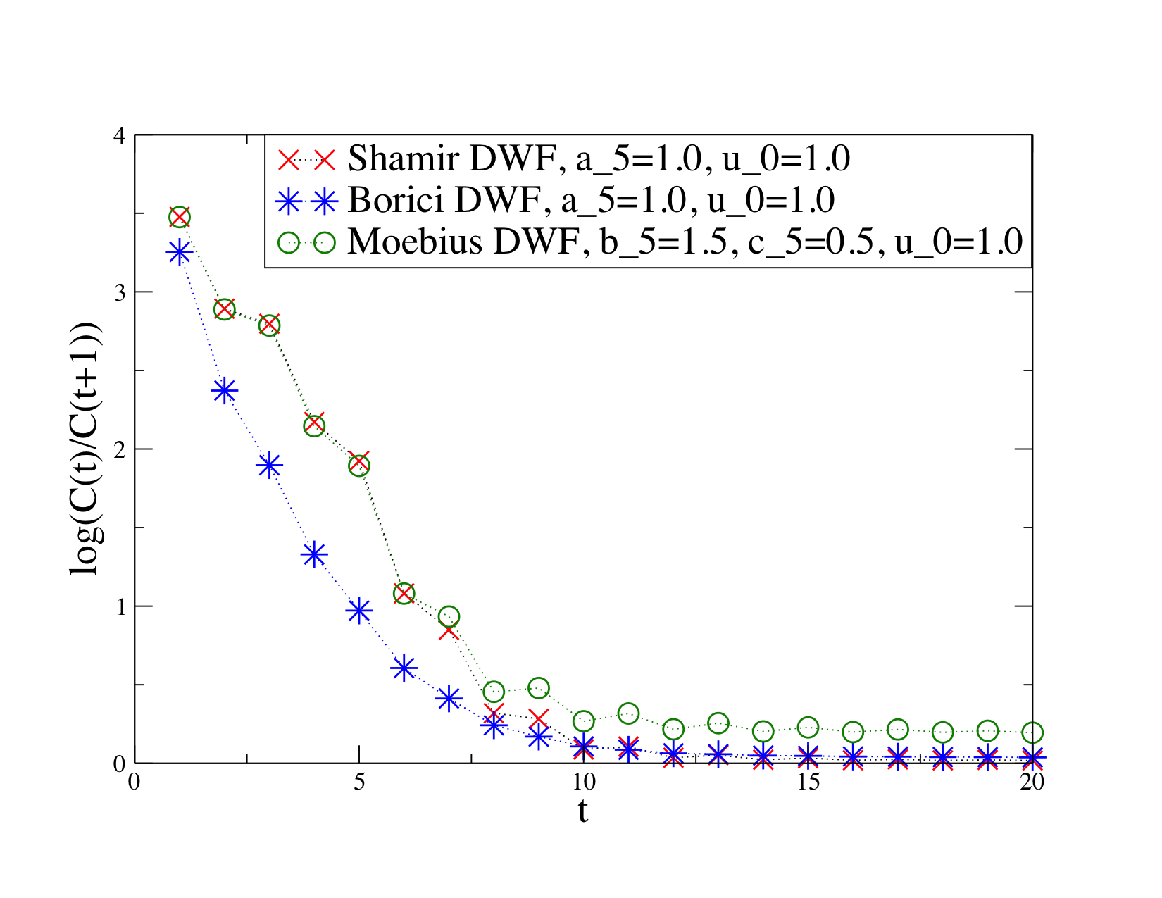
Figure 1: $m_{eff}$ plot for $M=1.8$, $m=0.005$, $a_{5}=1.0$, $b_{5}-c_{5}=1.0$, $u_{0}=1.0$, $L_{s}=16.$

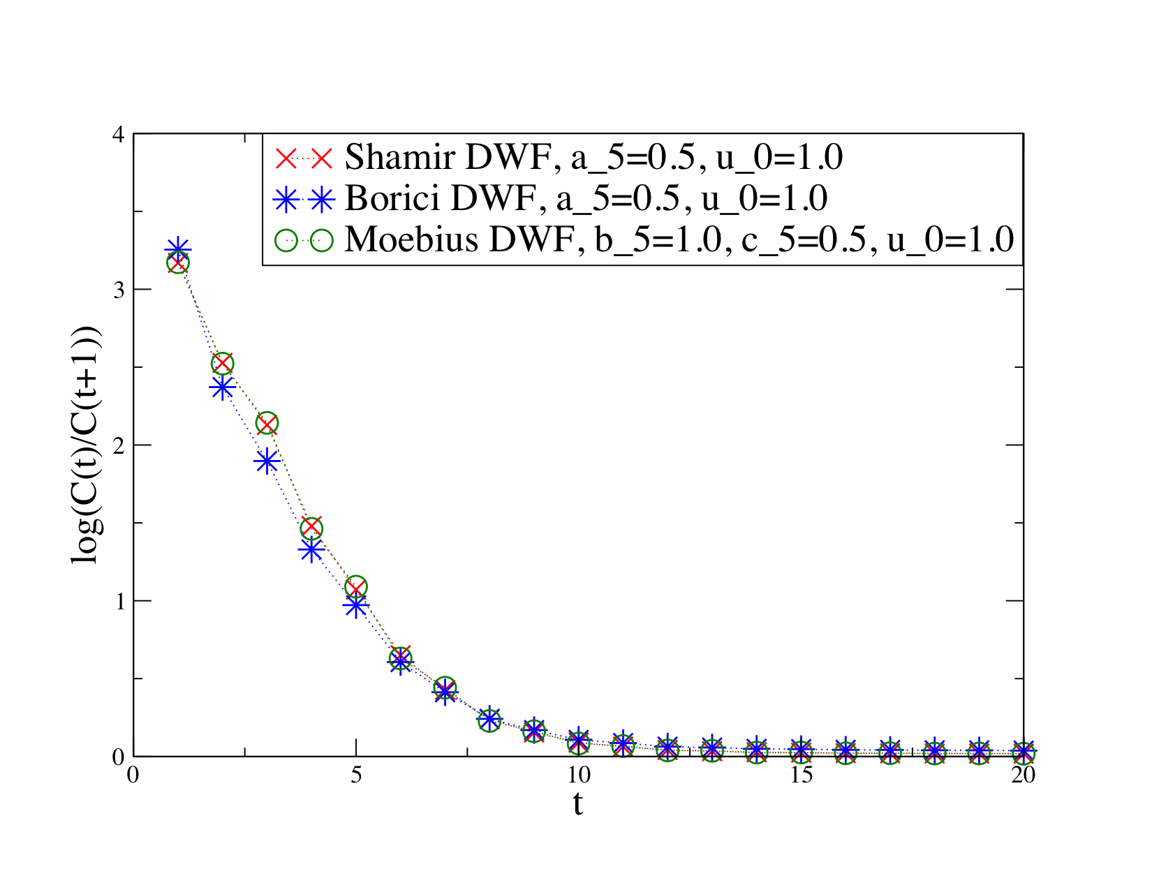
Figure 2: $m_{eff}$ plot for $M=1.8$, $m=0.005$, $a_{5}=0.5$, $b_{5}-c_{5}=0.5$, $u_{0}=1.0$, $L_{s}=16.$

An important observation to be made from from Figure 1 and Figure 2 is that the effective mass plot of Boriçi DWF exhibits almost zero or very little deviation from the expected exponential decay compared to Shamir and Möbius DWFs. We also point out that the effective mass plot remains the same for $a_{5}=1$ and $a_{5}=0.5$ for the Boriçi DWF in Figure 2 We see that the effective mass plot is rather insensitive to change in $a_{5}$ for the Boriçi DWF.

However, we notice from Figure 1 that the plateau of the effective mass plot of the Möbius DWF does not coincide with those of Shamir and Boriçi DWF. We see, if we increase $L_{s}$ from $L_{s}=16$ to $L_{s}=32$, all the plateaus coincide in the effective mass plots as shown in Figure 3 for $L_{s}=32$.

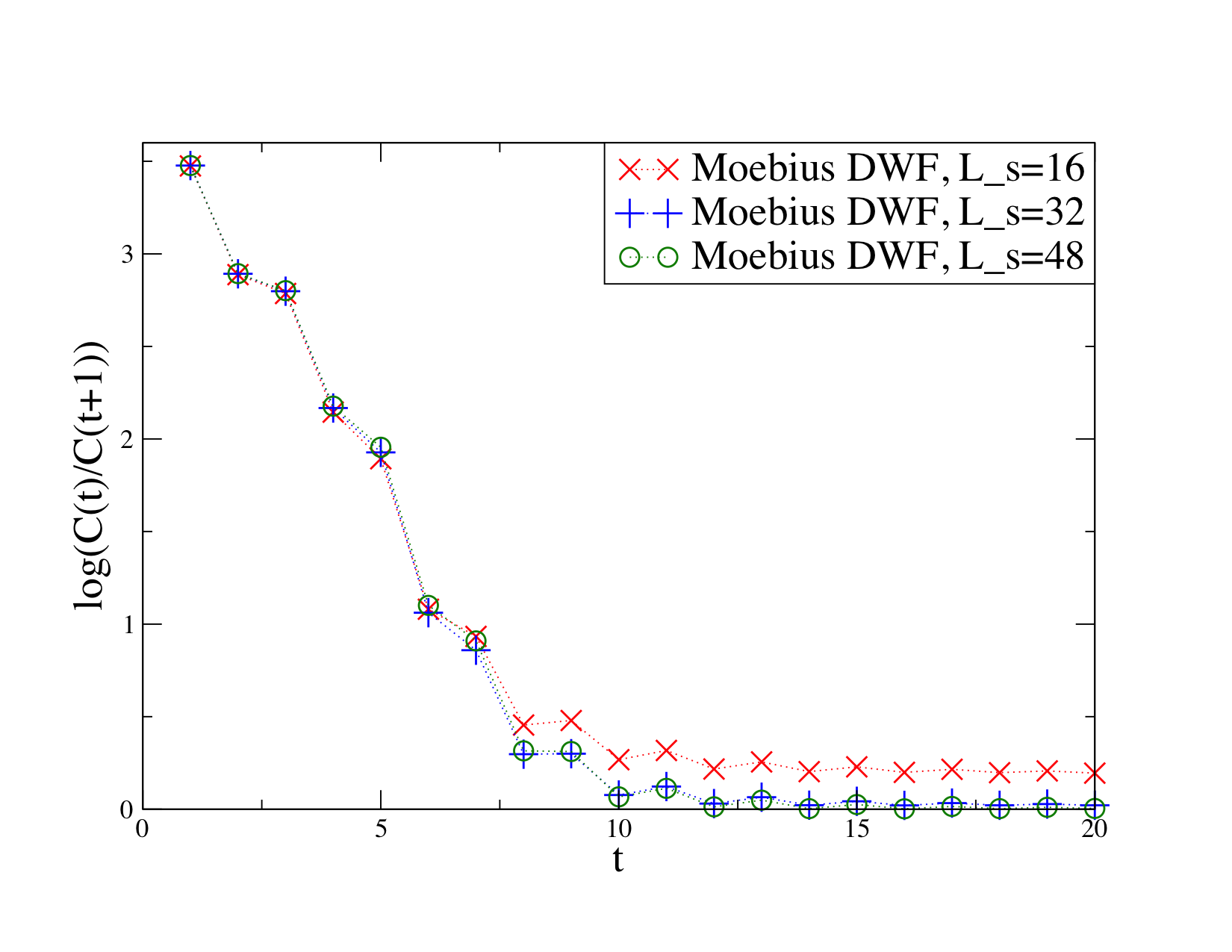
Figure 3: $m_{eff}$ plot for Möbius DWF. $M=1.8$, $m=0.005$, $b_{5}-c_{5}=1.0$, $u_{0}=1.0$, $L_{s}=16,32,48.$

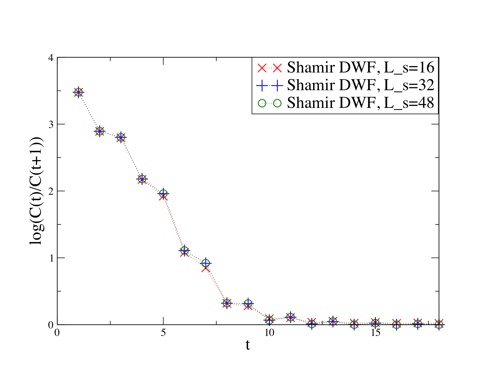
Figure 8: $m_{eff}$ plot for Shamir DWF. $M=1.8$, $m=0.005$, $a_{5}=1.0$, $u_{0}=1.0$, $L_{s}=16,32,48.$

Similar effective mass plots for different values of $L_{s}$ for Shamir and Boriçi DWFs can be found in Appendix B. It is interesting to notice from Figure 3 (also from Figures 8, 9) that the feature of oscillation in the effective mass plots remains same if one increases $L_{s}$ gradually from $L_{s}=16$ to $L_{s}=48$. This is consistent with the results in Table 2 that the unphysical pole disappears from the theory only when $L_{s}\to\infty$.

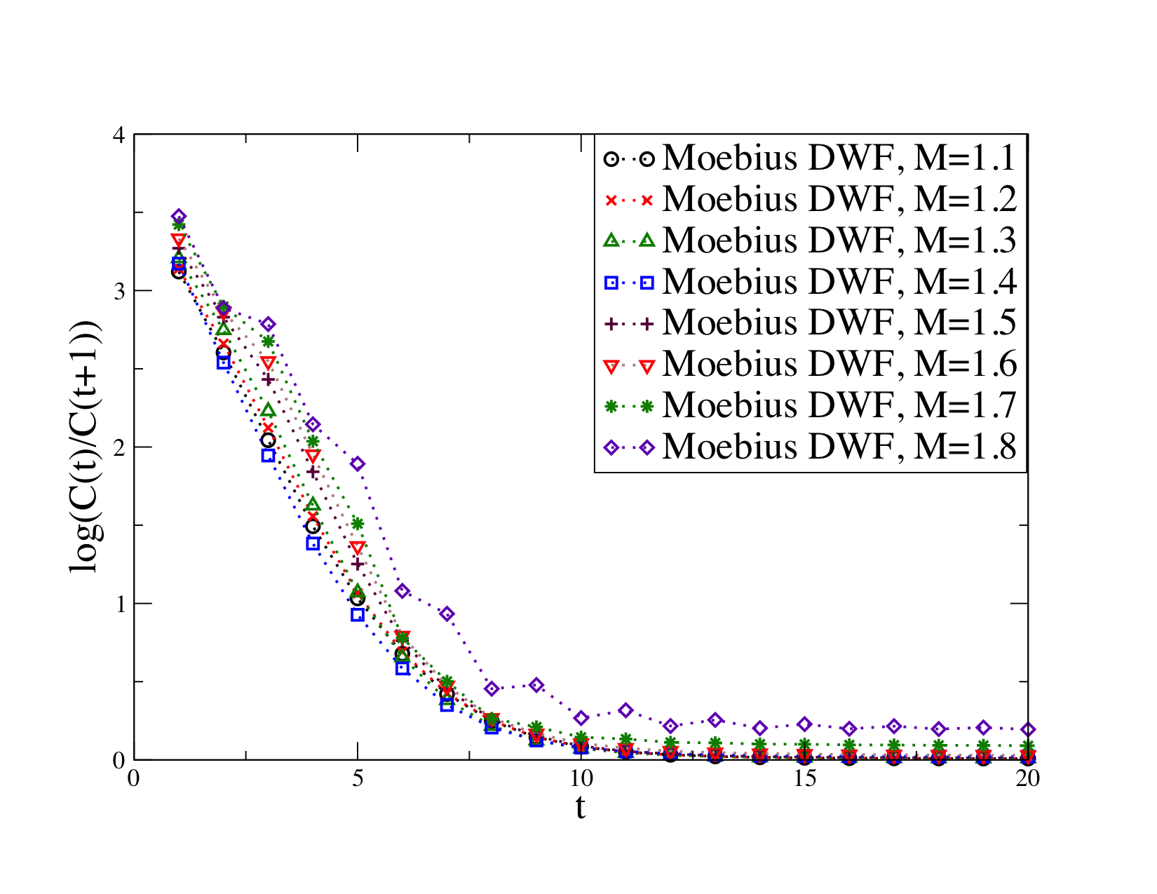
Figure 10: $m_{eff}$ plot for Möbius DWF. $M=1.1,1.2,....,1.8$, $m=0.005$, $b_{5}-c_{5}=1.0$, $u_{0}=1.0$, $L_{s}=16.$

We now compare the effective mass plots for different values of $M=1.1,1.2,....,1.8$. From Figure 4 we see that at earlier time slices the value of $\log(C(t)/C(t+1))$ increases as $M$ increases for Shamir DWF. From Figure 5, we notice at $t=1$, the value of $\log(C(t)/C(t+1))$ decreases as $M$ increases for Boriçi DWF. A similar graph for Möbius DWF has been presented in Appendix B (Figure 10). We note that the variation of the $\log(C(t)/C(t+1))$ curves as a function of $M$ for Boriçi DWF is much smaller than both the Shamir (Figure 4) as well as the Möbius DWF (Figure 10). This indicates that the extraction of excited states might be very sensitive to the values of $M$ when Shamir and Möbius DWFs are used for numerical simulation.

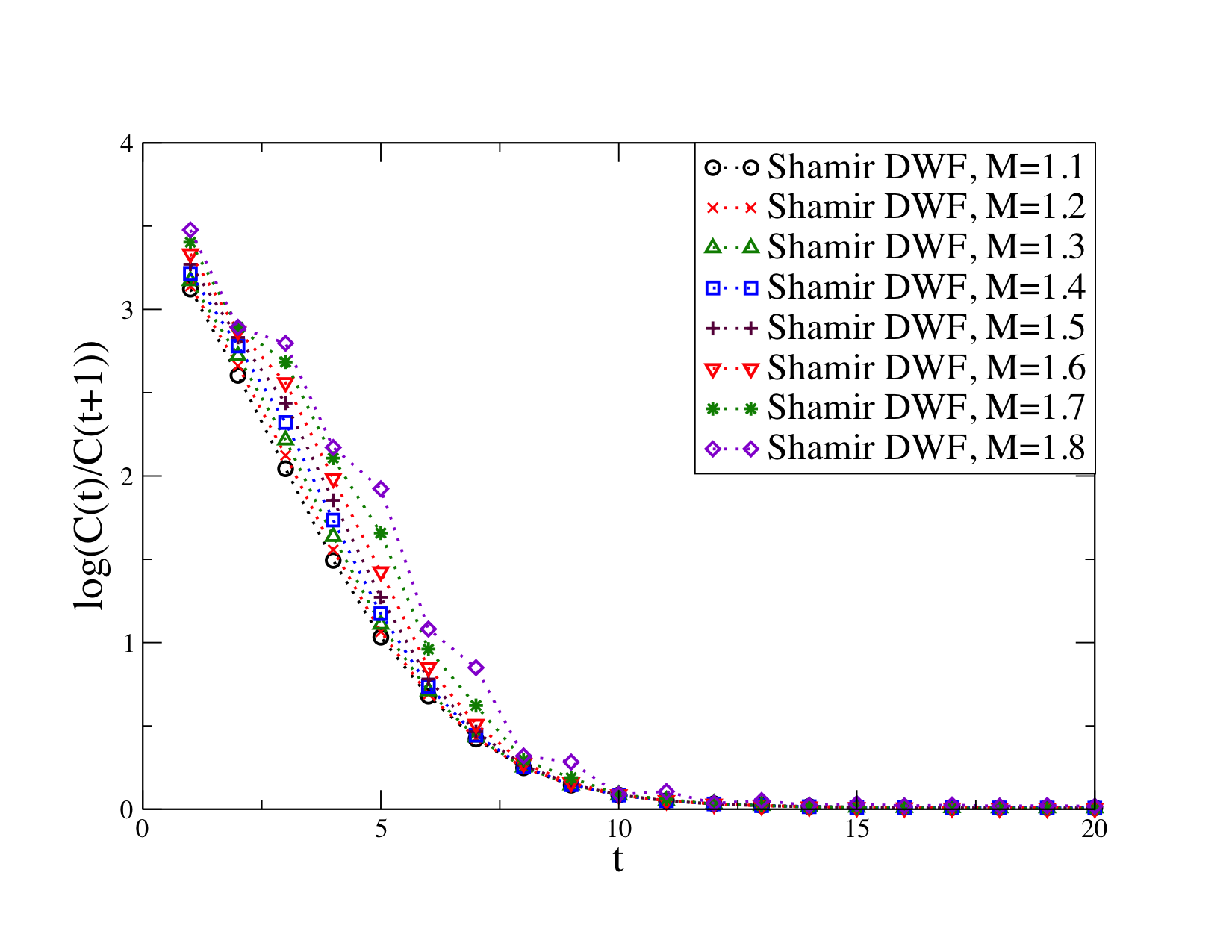
Figure 4: $m_{eff}$ plot for Shamir DWF. $M=1.1,1.2,.....,1.8$, $m=0.005$, $a_{5}=1.0$, $u_{0}=1.0$, $L_{s}=16.$

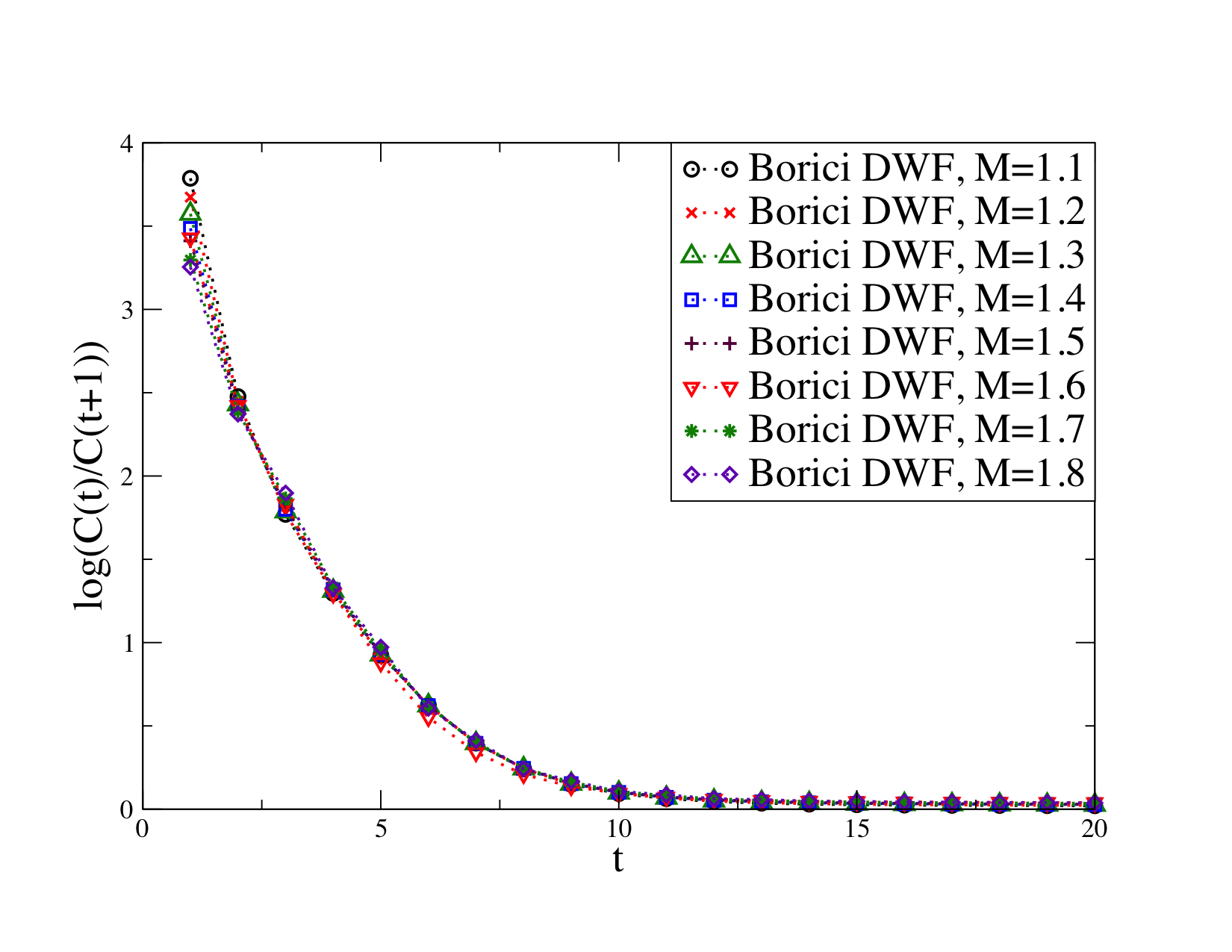
Figure 5: $m_{eff}$ plot for Boriçi DWF. $M=1.1,1.2,.....,1.8$, $m=0.005$, $a_{5}=1.0$, $u_{0}=1.0$, $L_{s}=16.$

We next consider the case where the fermion fields are coupled to a mean gauge field. Here, the links are replaced by their vacuum expectation value, $u_{0}$. We choose average plaquette value $P=0.58813$ Boyle . The mean field value of domain wall height is

$$M^{MF}=M-4(1-P^{\frac{1}{4}}).$$ (47)

Then for $M=1.8$ the value of $M^{MF}\approx 1.302$. $P=0.58813$ corresponds to a mean field $u_{0}\approx 0.85$ according to Aoki5 . According to the discussion in Ying , we observe the oscillations in the effective mass plot reduce with the mean field present. This result is presented in Figure 6.

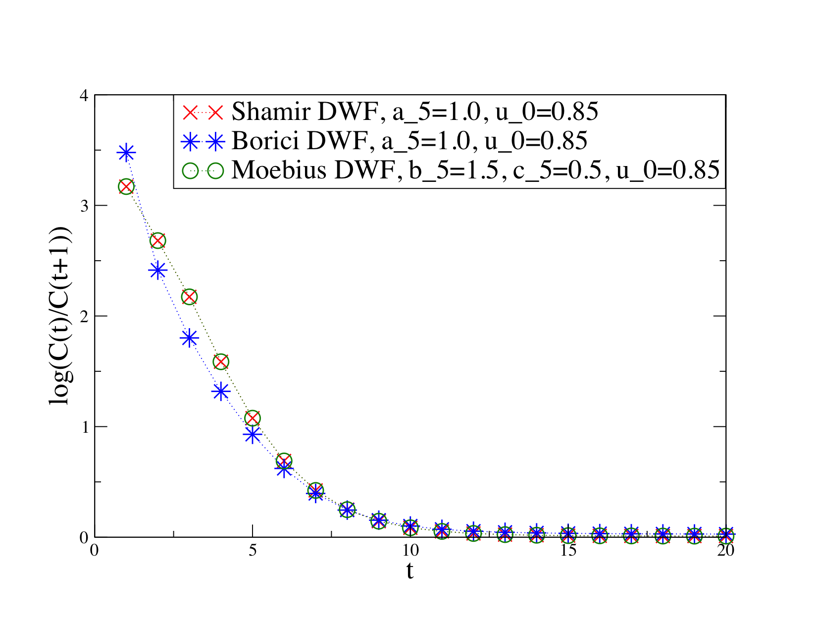
Figure 6: $m_{eff}$ plot for $M=1.8$, $m=0.005$, $a_{5}=1.0$, $b_{5}-c_{5}=1.0$, $u_{0}=0.85$, $L_{s}=16.$

We note that in Figures 1, 2, 5 and 6, the oscillation in the effective mass plot for the Boriçi DWF is nearly absent. The numerical simulations show clear evidence that Boriçi’s DWF exhibits minimal deviation from exponential decay at early time slices. However the tree level expressions for the unphysical pole are identical for every DWF action considered. To explain this fact, we consider the eigenmode expansion of the DWF propagator near the static mode (where $p_{i}=0$, and $p_{4}\neq 0$). The poles of $(\Omega^{0}_{s,s^{\prime}})^{-1}$ correspond to the solution $p^{0}_{4}$ which satisfies the condition,

$$\text{Det}\,\bigg{(}\Omega^{0}_{s,s^{\prime}}(p^{0}_{4})\bigg{)}=0.$$ (48)

For values of $p_{4}$ near the solution $p_{4}^{0}$, the propagator can be written as an eigendecomposition,

$$(\Omega^{0}_{s,s^{\prime}})^{-1}(p_{4})=\frac{1}{\lambda_{0}(p_{4})}V^{0}_{s}(p_{4})V^{0\dagger}_{s^{\prime}}(p_{4})+\sum_{i=1,2,..}\frac{1}{\lambda_{i}(p_{4})}V^{i}_{s}(p_{4})V^{i\dagger}_{s^{\prime}}(p_{4})$$ (49)

where $\Omega_{s,s^{\prime}}^{0}(p_{4})V^{i}(p_{4})=\lambda_{i}(p_{4})V^{i}(p_{4})$ and $\lambda_{0}(p_{4})$ is the eigenvalue of $\Omega_{s,s^{\prime}}^{0}(p_{4})$ which is the eigenvalue nearest zero and $V^{i}(p_{4})$ is the corresponding eigenvector. When $p_{4}$ is very close to $p^{0}_{4}$, $\lambda_{0}(p_{4})$ approaches zero and the eigenvector $V^{0}(p_{4})$ approaches $V^{0}(p^{0}_{4})$. In this case,

$$(\Omega^{0}_{s,s^{\prime}})^{-1}(p_{4})\sim\frac{1}{\lambda_{0}(p_{4}^{0})}V^{0}_{s}(p_{4}^{0})V^{0\dagger}_{s^{\prime}}(p_{4}^{0})$$ (50)

We have shown analytically that the value of $p_{4}^{0}$ at the unphysical pole is the same for the Shamir, Boriçi and Möbius DWFs, namely $p_{4}^{0}=\ln(1-M)$. However we have observed numerically that the Boriçi DWF has the least amount of oscillation during early time slices.

As discussed in Ying , if the contribution of the 5D unphysical eigenmode vanishes at the 4D boundary, oscillating behavior impacting 4D physics will vanish also. We illustrate this by plotting components of the zero-mode eigenvector for a value of $p_{4}$ corresponding to the unphysical pole (see eq. (48)) in Figure 7 We have taken $M=1.3$, $m=0.001$, $a_{5}=1.0$, $b_{5}=1.5$, $c_{5}=0.5$ as parameters for the DWF transfer matrix. We observe that the $s=1$ and $s=16$ components of this eigenvector of the Boriçi DWF nearly vanish compared to the Shamir and Möbius DWFs, and therefore have minimal coupling to 4D physics. Eqs. (3)-(19) illustrate that the 4D propagator is the chiral projection of a product of $q(x)$ and the 5D wave function $\psi$ (s=1 or s=N). Therefore if the $s=N$ component of $\psi$ due to the unphysical mode nearly vanishes at the 4D boundary, then the unphysical modes have minimal coupling to the 4D physics. This analysis is in good agreement with our earlier $m_{eff}$ plots where we found the Boriçi DWF exhibits negligible oscillation in the hadron correlators as compared to the Shamir and Möbius DWF formalisms.

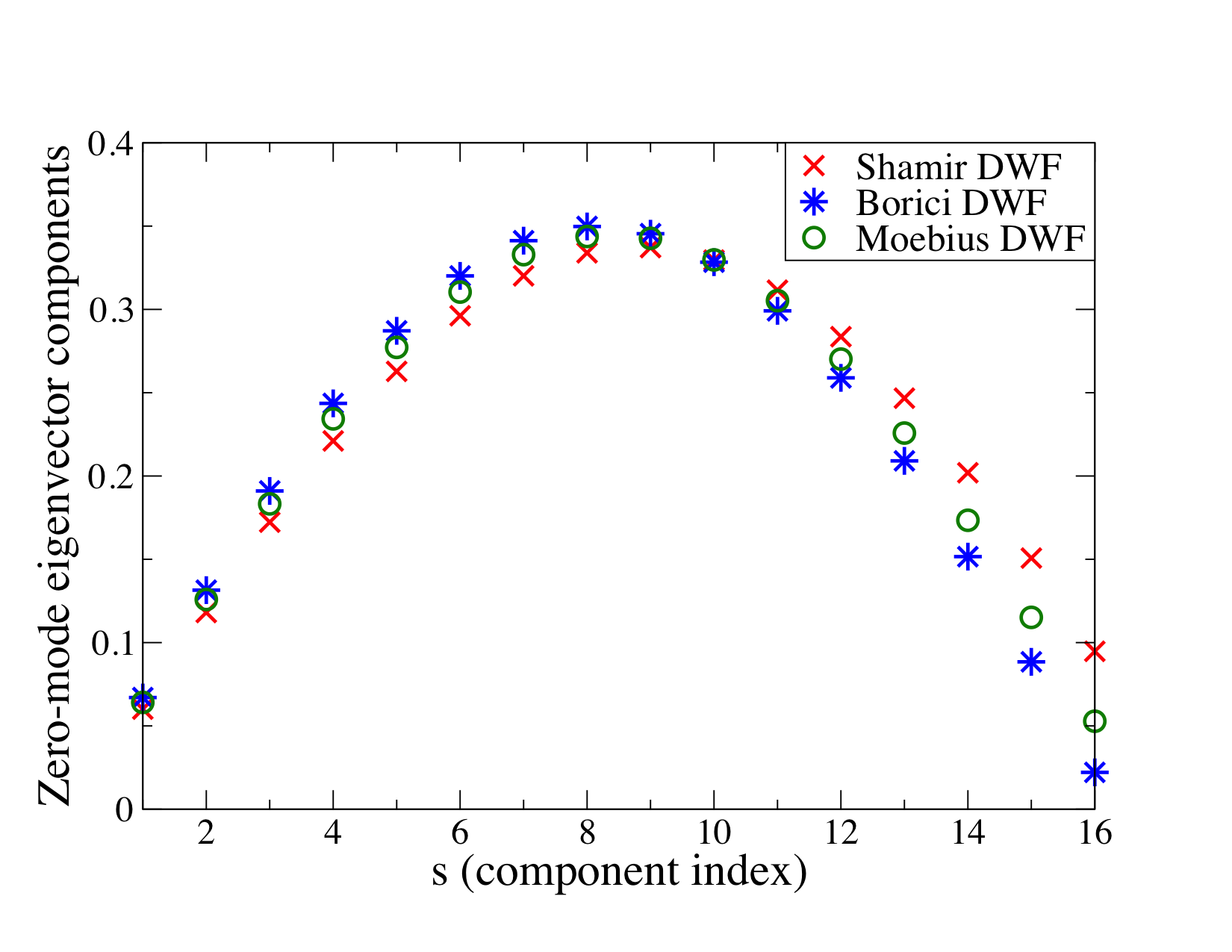
Figure 7: Unphysical zero-mode eigenvector components contribution at 4D boundary. $M=1.3$, $m=0.001$, $a_{5}=1.0$, $b_{5}=1.5$, $c_{5}=0.5$, $L_{s}=16$. The boundary at $L_{s}=16$ corresponds to the 4D boundary

7 Conclusions

In this work, we have provided a detailed analysis of the pole structure of the free propagator for the Shamir, Boriçi, and Möbius DWF actions. By investigating the poles we have provided a qualitative picture of the origin of oscillatory behavior in the effective mass plots when using DWFs and have quoted restrictions on the values of the product $Ma_{5}<1$ (Shamir, Boriçi), $M(b_{5}-c_{5})<1$ (Möbius) needed to ensure such oscillatory behavior is very small or absent for $M>1$. We have also pointed out that the Boriçi DWF correlators are insensitive to the change of values of $a_{5}$. We have shown for free case that at earlier time $\log(C(t)/C(t+1))$ curves for Shamir and Möbius DWFs depend significantly on the values of $M$. Therefore one needs to find out a value of $M$ such that extraction of hadron excited states produces the correct result.

In all cases, we observe that the Boriçi DWF has far less oscillatory effects at early time slices as compared to the other DWF actions we consider. We have argued why this is so by considering the contribution of unphysical eigenmodes on the 4D boundary of Boriçi DWF. We have shown that these eigenmodes are suppressed on the 4D boundary by a larger amount compared to Shamir and Möbius actions, which corresponds to smaller oscillatory effects contaminating the 4D physics of interest.

We have commented that the effects of the unphysical pole cannot be removed from the transfer matrix when realistic simulations are performed at a finite $L_{s}$. Because of this, the unphysical mode can have a significant impact on any fermion loop calculation when DWFs are employed. We close this section with the remark that even though this analysis represents a non-interacting analysis of the DWF pole structure, we expect similar qualitative features to be present in fully interacting calculations.

Appendix A Appendix A

The 4D Boriçi propagator in the momentum space:

$$S^{4D}(p) =i\not{\overline{p}}\Bigg{(}-\frac{m^{\prime 2}_{r}((c^{2}+\overline{p}^{2})(1-b^{\prime}e^{-\alpha^{\prime}})-m^{\prime 2}(1-be^{\alpha^{\prime}}))}{B^{\prime}F^{\prime}_{N}}+\frac{2m^{\prime 2}m^{\prime}_{r}}{F^{\prime}_{N}}+$$

$$\frac{m^{\prime 2}_{r}(c^{2}+\overline{p}^{2}-m^{\prime 2})(1-be^{\alpha^{\prime}})}{B^{\prime}F^{\prime}_{N}}-\frac{1}{B^{\prime}}-\frac{(c^{2}+\overline{p}^{2}-m^{\prime 2})(1-b^{\prime}e^{-\alpha^{\prime}})}{B^{\prime}F^{\prime}_{N}}$$

$$+\frac{m^{\prime 2}_{r}((c^{2}+\overline{p}^{2})(1-b^{\prime}e^{-\alpha^{\prime}})-m^{\prime 2}(1-b^{\prime}e^{\alpha^{\prime}}))}{B^{\prime}F^{\prime}_{N}}\Bigg{)}-b^{\prime}(p)\Bigg{(}\frac{m^{\prime}_{r}e^{\alpha}}{B^{\prime}}-\frac{m^{\prime}(m^{\prime 2}_{r}e^{\alpha}+e^{-\alpha})}{F^{\prime}_{N}}$$

$$-\frac{m^{\prime}_{r}e^{-\alpha}(c^{2}+\overline{p}^{2}-m^{\prime 2})(1-b^{\prime}e^{\alpha})}{B^{\prime}F^{\prime}_{N}}+\frac{m^{\prime 3}_{r}e^{\alpha}-m^{\prime}_{r}e^{-\alpha}((c^{2}+\overline{p}^{2})(1-b^{\prime}e^{-\alpha})-m^{\prime 2}(1-b^{\prime}e^{\alpha^{\prime}}))}{B^{\prime}F^{\prime}_{N}}\Bigg{)}$$

$$+m^{\prime}\Bigg{(}\frac{m^{\prime 2}_{r}((c^{2}+\overline{p}^{2})(1-b^{\prime}e^{-\alpha^{\prime}})-m^{\prime 2}(1-be^{\alpha^{\prime}}))}{B^{\prime}F^{\prime}_{N}}-\frac{m^{\prime 2}_{r}(c^{2}+\overline{p}^{2}-m^{\prime 2})(1-be^{\alpha^{\prime}})}{B^{\prime}F^{\prime}_{N}}+\frac{1}{B^{\prime}}$$

$$-\frac{2m^{\prime 2}m^{\prime}_{r}}{F^{\prime}_{N}}-\frac{(c^{2}+\overline{p}^{2}-m^{\prime 2})(1-b^{\prime}e^{-\alpha^{\prime}})}{B^{\prime}F^{\prime}_{N}}-\frac{m^{\prime 2}_{r}((c^{2}+\overline{p}^{2})(1-b^{\prime}e^{-\alpha^{\prime}})-m^{\prime 2}(1-b^{\prime}e^{\alpha^{\prime}}))}{B^{\prime}F^{\prime}_{N}}\Bigg{)}$$

where in the limit $a,a_{5}\to 1$ we have defined,

$$b^{\prime} =\left[-\overline{p}^{2}-b(p)c(p)\right]$$

$$m^{\prime} =-m(D_{w}(p)-1)$$

$$F_{N} =(c^{2}(p)+\overline{p}^{2})(1-b^{\prime}e^{\alpha^{\prime}})-m^{\prime 2}(1-b^{\prime}e^{-\alpha^{\prime}})$$

$$+m^{\prime}_{r}[4\sinh\alpha^{\prime}(c^{2}(p)+\overline{p}^{2}-m^{\prime 2})]$$

$$-m^{\prime 2}_{r}[(c^{2}(p)+\overline{p}^{2})(1-b^{\prime}e^{-\alpha^{\prime}})-m^{\prime 2}(1-b^{\prime}e^{\alpha^{\prime}})]$$

$$m^{\prime 2} =m^{2}(c^{2}(p)+\overline{p}^{2})$$

$$m^{\prime}_{r} =e^{-\alpha^{\prime}L_{s}}$$ (52)

Appendix B Appendix B

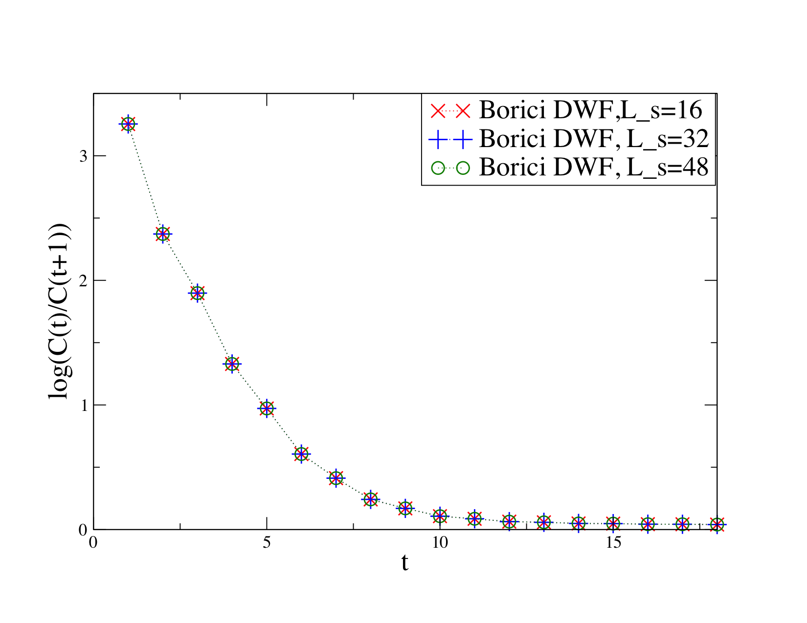
Figure 9: $m_{eff}$ plot for Boriçi DWF. $M=1.8$, $m=0.005$, $a_{5}=1.0$, $u_{0}=1.0$, $L_{s}=16,32,48.$

References

• (1) D. B. Kaplan, Phys. Lett. B 288 (1992) 342-347, [arXiv:hep-lat/9206013].
• (2) Y. Shamir, Nucl. Phys. B 406, 90 (1993).
• (3) J. J. Dudek, R. G. Edwards, and D. G. Richards, Phys. Rev. D 73, 074507 (2006) , [arXiv:hep-ph/0601137].
• (4) Y. Aoki et al. [RBC Collaboration], Phys. Rev. D 69, 074504 (2004), [arXiv:hep-lat/0211023].
• (5) Ph. Hagler et al. [LHPCCollaborations], Phys. Rev. D 77 (2008) 094502, [arXiv:0705.4295[hep-lat]].
• (6) A. Walker-Loud et al., Phys. Rev. D 79, 054502 (2009), [arXiv:0806.4549 [hep-lat]].
• (7) Y. Aoki et al., Phys. Rev. D 83, 074508 (2011), [arXiv:1011.0892 [hep-lat]].
• (8) S. Syritsyn and J. W. Negele, PoS(LAT2007) 078 (2007), [arXiv:0710.0425 [hep-lat]].
• (9) A. Borici, Nucl. Phys. Proc. Suppl. 83 (2000) 771, [arXiv:hep-lat/9909057].
• (10) R. C. Brower, H. Neff, and K. Orginos, Nucl. Phys. Proc. Suppl., 153 (2006) 191-198, [arXiv:hep-lat/0511031].
• (11) J. Liang, Y. Chen, M. Gong, L. Gui, K. F. Liu, Z. Liu, Y. B. Yang, Phys. Rev. D 89 (2014) 094507, [arXiv:1310.3532 [hep-lat]] .
• (12) X. Feng, X. Li, W. Liu, and C. Liu, JHEP 08 (2006) 060, [arXiv:hep-lat/0607021].
• (13) R. G. Edwards (LHPC Collaboration), B. Joo (UKQCD Collaboration), "The Chroma Soft ware System for Lattice QCD", arXiv:hep-lat/0409003, Proceedings of the 22nd International Symposium for Lattice Field Theory (Lattice2004), Nucl. Phys B 140 (Proc. Suppl) p832, 2005.
• (14) Yigal Shamir. Phys. Rev. D59 (1999) 054506, [hep-lat/9807012] .
• (15) T. Blum, A. Soni, Phys. Rev. D 56 (1997) 174, [hep-lat/9611030]; Phys. Rev. Lett. 79 3595, [hep-lat/9706023].
• (16) S. Aoki and Y. Taniguchi, Nucl. Phys. Proc. Suppl. 63 (1998) 290-292 .
• (17) Sinya Aoki, Taku Izubuchi, Yoshinobu Kuramashi and Yusuke Taniguchi Phys. Rev. D 59 (1999) 094505, [arXiv:hep-lat/9810020].
• (18) Sinya Aoki, Taku Izubuchi, Yoshinobu Kuramashi, Yusuke Taniguchi Phys. Rev. D 67 (2003) 094502, [arXiv:hep-lat/0603012].
• (19) G. P. Lepage, P. B. Mackenzie, Phys. Rev. D 48 (1993) 2250-2264, [arXiv:hep-lat/9209022] .
• (20) UKQCD Collaboration (P. A. Boyle (Edinburgh U.) et al.), Phys. Lett. B 641 (2006) 67-74 . Nucl. Phys. B 592 (2001) 183-202
• (21) Huey-Wen Lin, Nucl.Phys.Proc.Suppl. 187 (2009) 200-207, [arXiv:0812.0411 [hep-lat]].