Accretion Onto a Charged Higher-Dimensional Black Hole

Abstract

This paper deals with the steady-state polytropic fluid accretion onto a higher-dimensional Reissner-Nordstr$\ddot{o}$m black hole. We formulate the generalized mass flux conservation equation, energy flux conservation and relativistic Bernoulli equation to discuss the accretion process. The critical accretion is investigated by finding critical radius, critical sound velocity and critical flow velocity. We also explore gas compression and temperature profiles to analyze the asymptotic behavior. It is found that the results for Schwarzschild black hole are recovered when $q=0$ in four dimensions. We conclude that accretion process in higher dimensions becomes slower in the presence of charge.

Keywords: Accretion; Higher dimensional charged black hole.
PACS: 04.20.-q; 04.50.Gh; 04.25.dg.

1 Introduction

Black hole (BH) is one of the celestial objects having strong gravitational pull that the nearby matter even light cannot escape from its gravitational field. There are different ways to detect BH in binary systems and center of galaxies as it cannot be observed directly. The detection of its effect on the nearby matter is the one way and the most promising is accretion. In astrophysics, accretion is defined as the inward flow of matter surrounding a compact object under the influence of gravitational field. Recent developments in the study of quasars luminosity, relationship among masses of massive BHs and the properties of their host galaxies motivated the idea of accretion onto BHs [1].

Like most of the substances in the universe, all accreting matter is in gaseous form. The problem of gas accretion by a star was first studied by Hoyle and Lyttleton [2] and later by Bondi and Hoyle [3]. The steady-state spherically symmetric accretion was considered by Bondi [4] in which star was considered at rest at infinite gas cloud. In his classical model, he studied the flow of a barotropic fluid in the context of Newtonian gravity. Michel [5] extended this work in the framework of GR by investigating steady-state spherically symmetric inflow of gas onto Schwarzschild BH. Other important studies in this context are luminosity and frequency spectrum, the effect of magnetic field on accreting ionized gases and accretion onto a rotating BH [6]. Malec [7] investigated relativistic spherically symmetric accretion onto a BH with and without back reaction. He found that relativistic effects raise accretion mass in the absence of back reaction.

Shatskiy and Andreev [8] studied accretion onto a non-rotating compact object in comoving frame and explored dynamics of event horizon formation. Jamil et al. [9] analyzed the effect of phantom like dark energy onto Reissner-Nordstr$\ddot{o}$m (RN) BH and found that accretion is possible only through outer horizon. Jamil and Akbar [10] investigated accretion of exotic phantom energy onto $(2+1)$-dimensional Banados-Teitelboim-Zanelli (BTZ) BH and showed that mass accretion due to phantom energy is independent of BH mass. Babichev et al. [11] described steady-state spherically symmetric accretion of a perfect fluid as well as scalar field onto RN BH and found the formation of static atmosphere of fluid around naked singularity. The same authors [12] studied accretion of spherically symmetric metric with back reaction and showed that the metric is of Vaidya form near the horizon using perturbation. de Freitas Pacheco [13] examined relativistic as well as non-relativistic accretion onto RN BH using two equations of state (EOS) and found that accretion was slightly affected in the first case while in the second case it reduced upto 60% then the schwarzschild BH (for extreme RN case). Sharif and Abbas [14] investigated phantom accretion onto a magnetically stringy charged BH and found that BH does not transform into extremal BH or naked singularity.

Recently, Park and Ricotti [15] studied the increase in luminosity and growth rates of BHs moving at super sonic speed. Gaspari et al. [16] suggested that cooling rates are tightly linked to the BH accretion rates ($\dot{M}_{BH}\approx\dot{M}_{cool,core}$) in the galactic core. Karkowski and Malec [17] studied steady accretion onto BH that is immersed in a cosmological universe and found that dark energy may halt this type of accretion. Babichev et al. [18] investigated the interaction of dark energy with Schwarzschild as well as RN BH and gave physical reasons of decrease in mass due to accretion of phantom energy. Ganguly et al. [19] examined the process of accretion on $4$-dimensional string cloud and found an increase in the accretion rate with respect to string cloud parameter.

The study of gravity in a theory such as braneworld (which implies the existence of extra dimensions) has attracted many people from the last few decades. This theory is based on the fact that ($3+1$)-dimensional brane is embedded in a ($4+n$)-dimensional spacetime with $n$ compact spacelike dimensions [20]. It is suggested that in braneworld theory, the effects of quantum gravity can be observed in laboratory at TeV energies. Also, these theories recommend that higher-dimensional BHs can be produced in large hadron colliders and cosmic ray experiments. With the development of higher-dimensional theories [21], it would thus be interesting to study BHs in higher-dimensions

Tangherlini [22] was the pioneer in generalization of Schwarzschild BH in higher dimensions. Dadhich et al. [23] found the first static spherically symmetric BH solution in higher dimensions in the context of braneworld, which has the same structure as 4-dimensional RN BH. The physics of higher dimensional BH is much different and richer than in 4-dimensions [24]. Accretion in higher-dimensions onto TeV-scale BHs was first studied by Giddings and Mangano [25] in Newtonian background. Sharif and Abbas [26] investigated phantom energy accretion onto a 5-dimensional charged BH and found the validity of cosmic censorship hypothesis. John et al. [27] examined steady state accretion onto higher-dimensional Schwarzschild BH and found decrease in accretion mass. Debnath [28] studied accretion onto higher-dimensional charged BTZ BH assuming modified Chaplygin gas as accreting matter and found that initially BH mass increases and then decreases to a certain finite value for phantom stage.

In this paper, we study steady-state accretion onto a $D$-dimensional RN BH using the technique of Michel [5] as well as Shapiro and Teukolsky [29]. The paper is organized as follows: In section 2, we study analytic relativistic perfect fluid accretion onto RN BH in higher dimensions. Section 3 investigates accretion on critical points. We also study critical accretion with polytropic EOS and obtain expressions for gas compression and temperature profile near horizon. Finally, we summarize and discuss the results in the last section.

2 General Formalism for Spherical Accretion

In this section, we develop a general framework for accretion onto a higher-dimensional spacetime and study laws of conservation of mass and energy. The static spherically symmetric higher-dimensional RN BH is given by [30]

$$ds^{2}=-f(r)dt^{2}+f^{-1}(r)dr^{2}+r^{2}(d\Omega^{2}_{D-2}),$$ (1)

where $D$ is the spacetime dimension and

$$d\Omega^{2}_{D-2}=d\theta^{2}_{1}+\sin^{2}\theta_{1}d\theta^{2}_{2}+\sin^{2}\theta_{1}\sin^{2}\theta_{2}d\theta^{2}_{3}+...+\prod^{D-3}_{\mu=1}\sin^{2}\theta_{\mu}d\theta^{2}_{D-2}$$

is the line element on $(D-2)$-dimensional unit sphere whose volume is

$$\Omega_{D-2}=\frac{2\pi^{\frac{D-1}{2}}}{\Gamma(\frac{D-1}{2})}.$$

The lapse function in terms of mass and charge parameters $\mu$ and $q$ is

$$f(r)=1-\frac{2\mu}{r^{D-3}}+\frac{q^{2}}{r^{2(D-3)}},$$

where $\mu=\frac{8\pi GM}{(D-2)\Omega_{(D-2)}}$ and $q=\sqrt{\frac{8\pi G}{(D-2)(D-3)}}Q$ are the ADM mass and charge, respectively. When $q^{2}>\mu^{2}$, this solution develops singularity at $r=0$ while for $q^{2}\leq\mu^{2}$, $f(r)$ has two real roots

$$r_{\pm}=(\mu\pm\mu\sqrt{1-\frac{q^{2}}{\mu^{2}}})^{\frac{1}{(D-3)}},$$

where $r_{+}$ is the outer horizon and $r_{-}$ is the Cauchy horizon.

We consider steady-state inflow of gas onto central mass of BH in radial direction. The gas is assumed to be a perfect fluid specified by the energy-momentum tensor

$$T^{\sigma\upsilon}=(\rho+p)u^{\sigma}u^{\upsilon}+pg^{\sigma\upsilon}.$$ (2)

Here $p$ and $\rho$ are the pressure and energy density of the fluid and $u^{\sigma}=\frac{dx^{\sigma}}{ds}$ is the fluid $D$-velocity which satisfies the normalization condition $u^{\sigma}u_{\sigma}=-1$. We also define the baryon number flux $J^{\sigma}=nu^{\sigma}$, where $n$ is the proper baryon number density. The accretion process depends upon two laws of conservation. If no particles are created or destroyed then the particle number is conserved, i.e.,

$$\nabla_{\sigma}J^{\sigma}=\nabla_{\sigma}(nu^{\sigma})=0.$$ (3)

The law of conservation of energy-momentum tensor gives

$$\nabla_{\sigma}T^{\sigma}_{\upsilon}=0.$$ (4)

The non-zero components of D-velocity are $u^{0}=\frac{dt}{ds}$ and $\nu(r)=u^{1}=\frac{dr}{ds}$. Using $u^{\sigma}u_{\sigma}=-1$, we have

$$u^{0}=\frac{(\nu^{2}+1-\frac{2\mu}{r^{d-3}}+\frac{q^{2}}{r^{2(d-3)}})^{\frac{1}{2}}}{1-\frac{2\mu}{r^{D-3}}+\frac{q^{2}}{r^{2(D-3)}}}.$$

For $D$-dimensional RN BH, Eq.(3) takes the form

$$\frac{1}{r^{D-2}}\frac{d}{dr}(r^{D-2}n\nu)=0.$$ (5)

The null and radial components of Eq.(4) can be written as

$$\frac{1}{r^{D-2}}\frac{d}{dr}[r^{D-2}\nu(\rho+p)(\nu^{2}+1-\frac{2\mu}{r^{D-3}}+\frac{q^{2}}{r^{2(D-3)}})^{\frac{1}{2}}]=0,$$ (6)

$$\nu\frac{d\nu}{dr}=-\left[\frac{dp}{dr}(\frac{\nu^{2}+1-\frac{2\mu}{r^{D-3}}+\frac{q^{2}}{r^{2(D-3)}}}{\rho+p})+(D-3)(\frac{\mu}{r^{D-2}}-\frac{q^{2}}{r^{2D-5}})\right].$$ (7)

For $q=0$ and $D=4$, the above equations reduce to the expressions for the Schwarzschild BH [5, 29].

3 Critical Accretion

This section is devoted to study the solutions passing through critical points that describe the material falling into BH with increasing velocity. The behavior of falling fluid at critical points can express a variety of changes close to the compact objects. The speed of sound in the medium is also very important for a fluid as shown in the classical paper by Bondi [4]. We consider an adiabatic fluid for which there is no entropy production, hence the law of conservation of mass energy is defined as [29]

$$TdS=0=d(\frac{\rho}{n})+pd(\frac{1}{n}),$$ (8)

where $S$ is the entropy per baryon and $T$ is the temperature. It may be written as $\frac{d\rho}{dn}=\frac{\rho+p}{n}$, leading to the adiabatic sound speed $\alpha$

$$\alpha^{2}\equiv\frac{dp}{d\rho}=\frac{n}{\rho+p}\frac{dp}{d\rho}.$$ (9)

Using this equation, the baryon and energy-momentum conservation become

$$\frac{\nu^{\prime}}{\nu} + \frac{n^{\prime}}{n}+\frac{D-2}{r}=0,$$ (10)

$$\nu\nu^{\prime} + \alpha\frac{n^{\prime}}{n}(1-\frac{2\mu}{r^{D-3}}+\frac{q^{2}}{r^{2(D-3)}}+\nu^{2})+(D-3)(\frac{\mu}{r^{D-2}}-\frac{q^{2}}{r^{2D-5}})=0,$$

where prime denotes differentiation with respect to $r$. Using Eqs.(10) and (3), we obtain

$$\nu^{\prime}=\frac{X_{1}}{X},\quad n^{\prime}=\frac{X_{2}}{X},$$ (12)

where

$$X_{1} = \frac{1}{n}\left[\frac{\alpha(D-2)}{r}(\nu^{2}+1-\frac{2\mu}{r^{D-3}}+\frac{q^{2}}{r^{2(D-3)}})-(D-3)(\frac{\mu}{r^{D-2}}-\frac{q^{2}}{r^{2D-5}})\right],$$

$$X_{2} = -\frac{1}{\nu}\left[\frac{\nu^{2}(D-2)}{r}-(D-3)(\frac{\mu}{r^{D-2}}-\frac{q^{2}}{r^{2D-5}})\right],$$ (14)

$$X = \frac{\nu^{2}-\alpha(\nu^{2}+1-\frac{2\mu}{r^{D-3}}+\frac{q^{2}}{r^{2(D-3)}})}{\nu n}.$$ (15)

For large values of $r$ ($r\rightarrow\infty$), the flow satisfies $\nu^{2}\ll 1$ and is subsonic ($\nu^{2}<\alpha^{2}$) while the sound speed must be sub-luminal ($\alpha^{2}<1$), thus Eq.(15) implies that

$$X\simeq\frac{\nu^{2}-\alpha^{2}}{\nu n}<0.$$ (16)

At the event horizon, we have

$$X=\frac{\nu^{2}(1-\alpha^{2})}{\nu n}>0,$$ (17)

under the causality constraint $\alpha^{2}<1$. It is mentioned here that Eq.(17) is possible only for the extreme RN case, i.e., for $q=\mu$. From Eq.(16) and (17), we see that $X$ must pass through zero at $r=r_{c}$. A flow with constant energy and entropy must be smooth at every point. Thus, if denominator vanishes at some point, the numerator must also vanish at that point, so for a smooth flow we must have $X_{1}=X_{2}=X=0$ at $r=r_{c}$ [29]. From Eqs.(3)-(15), we obtain a relationship between flow and sound velocity as

$$\nu^{2}_{c}=\frac{\alpha^{2}_{c}(1-\frac{q^{2}}{r^{2(D-3)}})}{1+\alpha^{2}_{c}(\frac{D-1}{D-3})}=\frac{D-3}{D-2}(\frac{\mu}{r^{D-3}}-\frac{q^{2}}{r^{2(D-3)}}),$$ (18)

where $\nu_{c}\equiv\nu(r_{c})$ and $\alpha_{c}\equiv\alpha(r_{c})$. In the absence of charge parameter in four-dimensions, the above relation is exactly the same as obtained in [27]. To determine the accretion rate $\dot{M}$, we integrate Eq.(5) over a $(D-1)$-dimensional volume and multiply by the baryon mass, $m_{b}$, it follows that

$$\dot{M}=\frac{2\pi^{\frac{D-1}{2}}}{\Gamma(\frac{D-1}{2})}r^{D-2}m_{b}n\nu,$$ (19)

where $\dot{M}$ is the constant of integration (independent of $r$, having dimension of mass per unit time), related to mass accretion rate [4]. Equation (19) is the generalization of the Bondi’s accretion rate in higher-dimensions. For $q=0$ and $D=4$, it reduces to the Schwarzschild case.

Following [18], Eqs.(5) and (6) lead to

$$n\nu r^{D-2} = A,$$ (20)

$$(\frac{\rho+p}{n})^{2}(1-\frac{2\mu}{r^{D-3}}+\frac{q^{2}}{r^{2(D-3)}}) = (\frac{\rho_{\infty}+p_{\infty}}{n_{\infty}})^{2},$$ (21)

where $A$ is the constant of integration. Differentiating Eqs.(20) and (21) and eliminating $d\rho$, we have

$$\frac{d\nu}{dr}=-\frac{\nu}{r}\frac{\left[V^{2}-\frac{\nu^{2}}{1-\frac{2\mu}{r^{D-3}}+\frac{q^{2}}{r^{2(D-3)}}+\nu^{2}}\right]}{\left[(D-2)V^{2}-\frac{(D-3)(\frac{\mu}{r^{D-3}}-\frac{q^{2}}{r^{2(D-3)}})}{1-\frac{2\mu}{r^{D-3}}+\frac{q^{2}}{r^{2(D-3)}}+\nu^{2}}\right]},$$ (22)

where $V^{2}\equiv\frac{dln(\rho+p)}{dn}-1$, which is equal to sound velocity $\frac{dp}{d\rho}=\alpha^{2}_{c}$ . Equation (21) is the generalized Bernoulli equation in $D$-dimensions for a charged BH. Equating numerator and denominator to zero, we obtain Eq.(18) and

$$V^{2}=\alpha^{2}_{c}=\frac{(D-3)(\mu r^{D-3}-q^{2})}{(D-2)r^{2(D-3)}-(D-1)\mu r^{D-3}+q^{2}}.$$ (23)

Equation (23) yields the critical radius as

$$r^{D-3}_{c}=\frac{\mu\alpha^{2}_{c}(D-1)+(D-3)}{2\alpha^{2}_{c}(D-2)}\left[1\pm\left[1-\frac{4\alpha^{2}_{c}(D-2)(D-3+\alpha^{2}_{c})}{\alpha^{2}_{c}(D-1)+(D-3)}\frac{q^{2}}{\mu^{2}}\right]^{\frac{1}{2}}\right].$$ (24)

This equation leads to two possible solutions for the critical radius corresponding to $+$ and $-$ signs. The first indicates the critical radius outside the event horizon which is a physically acceptable solution. The second possibility shows the critical radius between inner and outer horizons [9]. In the present analysis, we are interested only in the first solution. In the limit $D=4$, our results correspond to [13, 18].

3.1 Accretion with Polytropic Equation of State

The physical state of homogeneous substance can be described by EoS. In order to determine an explicit value of $\dot{M}$ as well as all the fundamental characteristics of flow, Eqs.(19) and (21) must be analyzed using EoS. We consider the polytropic EoS

$$p=kn^{\omega},$$ (25)

where $k$ is constant and $\omega$ is adiabatic index satisfying $1<\omega<\frac{5}{3}$. Inserting Eq.(25) into (8) and integrating, we obtain

$$\rho=\frac{k}{\omega-1}n^{\omega}+m_{b}n,$$ (26)

where $m_{b}$ is the constant of integration obtained by comparing with total energy density $\rho=m_{b}n+\varepsilon$, $m_{b}n$ is the rest mass-energy density and $\varepsilon$ is the internal energy density. From Eqs.(25) and (26), we have

$$\omega kn^{\omega-1}=\frac{m_{b}\alpha^{2}}{1-\frac{\alpha^{2}}{\omega-1}}.$$ (27)

When $\frac{\alpha^{2}}{\omega-1}\ll 1$, we have $n\sim\alpha^{\frac{2}{\omega-1}}$ [29], leading to

$$\frac{n_{c}}{n_{\infty}}\approx(\frac{\alpha_{c}}{\alpha_{\infty}})^{\frac{2}{\omega-1}}.$$ (28)

Using Eq.(25) and (26) in (21), it follows that

$$(1+\frac{\alpha^{2}}{\omega-1-\alpha^{2}})^{2}(1-\frac{2\mu}{r^{D-3}}+\frac{q^{2}}{r^{2(D-3)}}+\nu^{2})=(1+\frac{\alpha^{2}_{\infty}}{\omega-1-\alpha^{2}_{\infty}})^{2}.$$ (29)

At critical radius, using (18) and inverting Eq.(29), we obtain

$$(1-\frac{\alpha^{2}_{c}}{\omega-1})^{2}(\frac{(D-3)+\alpha^{2}_{c}(D-1)}{D-3})=(1-\frac{\alpha^{2}_{\infty}}{\omega-1})^{2},$$ (30)

For large values of $r$ ($r>r_{c}$), the baryons are expected to be non-relativistic ($T\ll mc^{2}/\texttt{k}=10^{13}\texttt{K}$), where k and K are Planck length and Kelvin, respectively. In this system, we must have $\alpha\ll\alpha_{c}\ll 1$. Expanding Eq.(30), we obtain a relationship between sound velocity at critical point and the point at infinity as

$$\alpha^{2}_{c}\approx\frac{2\alpha^{2}_{\infty}(D-3)}{(3D-7)-\omega(D-1)},$$ (31)

which corresponds to [13] for $D=4$. Using Eq.(31), critical radius takes the form

$$r^{D-3}_{c} \approx \left[1+\left[\frac{(8\alpha^{2}_{\infty}(D-2)(D-3))((3D-7)-\omega(D-1)+2\alpha^{2}_{\infty})}{(2\alpha^{2}_{\infty}(D-1)-(2D-4))((2D-7)-\omega(D-1))}\frac{q^{2}}{\mu^{2}}\right]^{\frac{1}{2}}\right]$$ (32)

$$\times \frac{\mu((3D-7)-\omega(D-1))}{4\alpha^{2}_{\infty}(D-2)(D-3)}.$$

We evaluate Bondi mass accretion rate $\dot{M}$ at the critical point from Eq.(19) as follows

$$\dot{M}=\frac{2\pi^{\frac{D-1}{2}}}{\Gamma(\frac{D-1}{2})}r^{D-2}_{c}m_{b}n_{c}\nu_{c}=\frac{2\pi^{\frac{D-1}{2}}}{\Gamma(\frac{D-1}{2})}\lambda_{c}\mu^{\frac{D-2}{D-3}}m_{b}n_{\infty}\alpha^{-(\frac{D-1}{D-3})}_{\infty}f(e),$$ (33)

where

$$\lambda_{c}=(\frac{D-3}{2})^{\frac{\omega+1}{2(\omega-1)}}\left(\frac{(3D-7)-\omega(D-1)}{4}\right)^{\frac{7-3D+\omega(D-1)}{2(D-3)(\omega-1)}}(D-2)^{\frac{2-D}{D-3}},$$ (34)

is dimensionless accretion parameter and

$$f(e) = \left[1+\left[\frac{(8\alpha^{2}_{\infty}(D-2)(D-3))((3D-7)-\omega(D-1)+2\alpha^{2}_{\infty})e^{2}}{(2\alpha^{2}_{\infty}(D-1)-(2D-4))((2D-7)-\omega(D-1))}\right]^{\frac{D-1}{4(D-3)}}\right]$$

$$\times \left[1-e^{2}\left[\frac{(3D-7)-\omega(D-1)}{4(D-2)(D-3)\alpha^{2}_{\infty}}\left[1\right.\right.\right.$$

$$+ \left.\left.\left.\left[\frac{(8\alpha^{2}_{\infty}(D-2)(D-3))((3D-7)-\omega(D-1)+2\alpha^{2}_{\infty})e^{2}}{(2\alpha^{2}_{\infty}(D-1)-(2D-4))((2D-7)-\omega(D-1))}\right]^{\frac{1}{2}}\right]\right]^{-1}\right],$$

here $e=\frac{q^{2}}{\mu^{2}}$. Re-writing Eq.(33) in terms of $G$ and $M$, we have

$$\dot{M} = \sqrt{\pi}[2^{\frac{4D-9}{D-3}}(D-2)^{-2(\frac{D-2}{D-3})}(\frac{D-1}{2})^{\frac{1}{D-3}}]$$ (36)

$$\times (GM)^{\frac{D-2}{D-3}}m_{b}n_{\infty}\alpha^{-(\frac{D-1}{D-3})}_{\infty}(\frac{D-3}{2})^{\frac{\omega+1}{2(\omega-1)}}$$

$$\times \left[\frac{3D-7-\omega(D-1)}{4}\right]^{\frac{7-3D+\omega(D-1)}{2(D-3)(\omega-1)}}f(e),$$

and

$$f(e) = \left[1+\left[\frac{(8\alpha^{2}_{\infty}(D-2)(D-3))((3D-7)-\omega(D-1)+2\alpha^{2}_{\infty})}{(2\alpha^{2}_{\infty}(D-1)-(2D-4))((2D-7)-\omega(D-1))}\right.\right.$$ (37)

$$\times \left.\left.\frac{\pi^{D-2}(D-2)Q^{2}}{2G(D-3)(\Gamma(\frac{D-1}{2})^{2})}\right]^{\frac{D-1}{4(D-3)}}\right]$$

$$\times \left[1-\frac{\pi^{D-2}(D-2)Q^{2}}{2G(D-3)(\Gamma(\frac{D-1}{2})^{2})}\left[\frac{(3D-7)-\omega(D-1)}{4(D-2)(D-3)\alpha^{2}_{\infty}}\left[1\right.\right.\right.$$

$$+ \left.\left.\left.\left[\frac{(8\alpha^{2}_{\infty}(D-2)(D-3))((3D-7)-\omega(D-1)+2\alpha^{2}_{\infty})}{(2\alpha^{2}_{\infty}(D-1)-(2D-4))((2D-7)-\omega(D-1))}\right.\right.\right.\right.$$

$$\times \left.\left.\left.\left.\frac{\pi^{D-2}(D-2)Q^{2}}{2G(D-3)(\Gamma(\frac{D-1}{2})^{2})}\right]^{\frac{1}{2}}\right]\right]^{-1}\right].$$

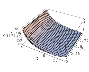
Figure 1: Plots of the accretion rate $\dot{M}$ as a function of $D=4-11$ and $\lambda_{c}$ for $\omega$=1.1, $\frac{4}{3}$, 1.6 and $e=0.2,0.4,0.64$.

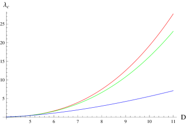
Figure 2: Behavior of accretion parameter $\lambda_{c}$ corresponding to $D=4-11$ where red, blue and green curves indicate $\omega$=1.1, $\frac{4}{3}$ and 1.6.

Equation (36) shows that accretion rate in charged background is modified by the term $f(e)$. However, the mass accretion rate scales as $\dot{M}\sim M^{\frac{D-2}{D-3}}$ which corresponds to the Newtonian [4] as well as relativistic model [29] for $e=0,~{}D=4$. For the standard values of adiabatic index ($1<\omega<\frac{5}{3}$), different values of $e$ and $G=1,~{}M=M_{{}_{\bigodot}}=1.989\times 10^{33}g$, $m_{b}=1.67\times 10^{-24}g$, $\alpha_{\infty}=10^{6}cms^{-1}$, $n_{\infty}=1cm^{-3}$, the behavior of $r_{c},~{}\lambda_{c}$ and $\dot{M}$ is given in Tables 1-7. The graphical representation of $\dot{M}$ and $\lambda_{c}$ is shown in Figures 1 and 2. It is seen that dimensions as well as charge parameter affect the rate of accretion. The accretion rate becomes slower as the dimension increases. The rate of accretion for small values of charge is higher as compared to large values. Thus $\dot{M}$ shows decreasing behavior for increasing dimensions as well as charge.

Table 1: Accretion parameter $\lambda_{c}$ for $\omega=1.2,~{}\frac{4}{3},~{}1.6$.

$D$	$\lambda_{c1}$	$\lambda_{c2}$	$\lambda_{c3}$
4	0.2488	0.1768	0.0917
5	0.4967	0.4330	0.3545
6	0.6004	0.5473	0.4818
7	0.6543	0.6077	0.5503
8	0.6868	0.6444	0.5922
9	0.7085	0.6689	0.6202
10	0.7239	0.6864	0.6403
11	0.7353	0.6994	0.6553

3.2 Asymptotic Analysis

Here we estimate the flow parameters for $r_{H}<r\ll r_{c}$ as well as $r=r_{c}$. The gas passes through supersonic flow at distance below Bondi radius, i.e., $\nu>\alpha$ when $r_{H}<r\ll r_{c}$. We find an upper bound of the radial dependence of gas velocity [27, 29]

$$\nu^{2}\approx\frac{2\mu}{r^{D-3}}-\frac{q^{2}}{r^{2(D-3)}}.$$ (38)

The gas compression rate from Eqs.(19), (33) and (38) becomes

$$\frac{n(r)}{n_{\infty}}\approx\frac{\lambda_{c}}{\sqrt{2}}f(e)(\frac{\mu}{r^{D-3}\alpha^{2}_{\infty}})^{\frac{D-1}{2(D-3)}}(1-\frac{q^{2}}{4\mu r^{D-3}}).$$ (39)

Table 2: Critical radius $r_{c}$ for $\omega=1.1$ and $e=0.2,~{}0.4,~{}0.67$.

$D$	$r_{c1}$	$r_{c2}$	$r_{c3}$
4	$9.8156\times 10^{26}$	$1.9631\times 10^{26}$	$3.2882\times 10^{26}$
5	$3.4519\times 10^{26}$	$6.9118\times 10^{26}$	$1.1577\times 10^{26}$
6	$1.7840\times 10^{25}$	$3.5681\times 10^{25}$	$5.9765\times 10^{25}$
7	$1.0928\times 10^{25}$	$2.1855\times 10^{24}$	$3.6607\times 10^{25}$
8	$7.3908\times 10^{25}$	$1.4782\times 10^{24}$	$2.4759\times 10^{24}$
9	$5.9955\times 10^{25}$	$1.0671\times 10^{24}$	$1.7874\times 10^{24}$
10	$3.4519\times 10^{24}$	$8.0682\times 10^{23}$	$1.3515\times 10^{23}$
11	$3.4519\times 10^{24}$	$6.3162\times 10^{23}$	$1.0580\times 10^{23}$

Table 3: Critical radius $r_{c}$ for $\omega=\frac{4}{3}$ and $e=0.2,~{}0.4,~{}0.67$.

$D$	$r_{c1}$	$r_{c2}$	$r_{c3}$
4	$9.1026\times 10^{26}$	$1.8205\times 10^{26}$	$3.0494\times 10^{26}$
5	$3.2566\times 10^{26}$	$6.5133\times 10^{26}$	$1.0910\times 10^{26}$
6	$1.6925\times 10^{26}$	$3.3850\times 10^{25}$	$5.6698\times 10^{25}$
7	$1.0405\times 10^{25}$	$2.0810\times 10^{25}$	$3.4857\times 10^{25}$
8	$7.0539\times 10^{25}$	$1.4108\times 10^{25}$	$2.3630\times 10^{24}$
9	$3.8662\times 10^{25}$	$1.0201\times 10^{24}$	$1.7087\times 10^{24}$
10	$3.0523\times 10^{24}$	$7.1221\times 10^{24}$	$1.2935\times 10^{23}$
11	$3.0351\times 10^{24}$	$6.60505\times 10^{23}$	$1.0135\times 10^{23}$

Table 4: Critical radius $r_{c}$ for $\omega=1.6$ and $e=0.2,0.4,0.67$.

$D$	$r_{c1}$	$r_{c2}$	$r_{c3}$
4	$8.4515\times 10^{26}$	$1.6903\times 10^{26}$	$2.8313\times 10^{26}$
5	$3.0663\times 10^{26}$	$6.1326\times 10^{26}$	$1.0272\times 10^{26}$
6	$1.6033\times 10^{26}$	$3.2067\times 10^{25}$	$5.6117\times 10^{25}$
7	$1.8910\times 10^{26}$	$1.9782\times 10^{25}$	$3.4618\times 10^{25}$
8	$6.7201\times 10^{25}$	$1.3440\times 10^{24}$	$2.3520\times 10^{24}$
9	$4.8665\times 10^{25}$	$9.7330\times 10^{24}$	$2.6183\times 10^{24}$
10	$3.6882\times 10^{24}$	$7.3764\times 10^{23}$	$1.8443\times 10^{23}$
11	$2.8922\times 10^{24}$	$5.7844\times 10^{23}$	$1.4461\times 10^{23}$

Table 5: Accretion rate $\dot{M}$ for $\omega=1.1$ and $e=0.2,~{}0.4,~{}0.67$.

$D$	$\dot{M}_{1}$	$\dot{M}_{2}$	$\dot{M}_{3}$
4	$3.5568\times 10^{40}$	$6.2876\times 10^{39}$	$1.9883\times 10^{37}$
5	$2.0451\times 10^{27}$	$5.1129\times 10^{26}$	$5.1129\times 10^{24}$
6	$9.7005\times 10^{22}$	$2.7221\times 10^{22}$	$3.9958\times 10^{20}$
7	$6.9321\times 10^{22}$	$2.0611\times 10^{20}$	$3.6657\times 10^{18}$
8	$3.4150\times 10^{19}$	$3.5568\times 10^{19}$	$2.0977\times 10^{17}$
9	$4.1980\times 10^{18}$	$1.3223\times 10^{18}$	$2.8499\times 10^{16}$
10	$8.3930\times 10^{17}$	$2.6878\times 10^{17}$	$6.1199\times 10^{15}$
11	$2.2132\times 10^{16}$	$7.1759\times 10^{16}$	$1.7028\times 10^{15}$

Table 6: Accretion rate $\dot{M}$ for $\omega=\frac{4}{3}$ and $e=0.2,~{}0.4,~{}0.67$.

$D$	$\dot{M}_{1}$	$\dot{M}_{2}$	$\dot{M}_{3}$
4	$7.0978\times 10^{37}$	$1.2547\times 10^{37}$	$1.9559\times 10^{38}$
5	$1.6580\times 10^{25}$	$4.1449\times 10^{24}$	$3.7304\times 10^{25}$
6	$1.2230\times 10^{21}$	$3.4321\times 10^{20}$	$2.5720\times 10^{21}$
7	$1.0816\times 10^{19}$	$3.2273\times 10^{18}$	$2.0681\times 10^{19}$
8	$6.0816\times 10^{18}$	$1.8721\times 10^{17}$	$1.2116\times 10^{18}$
9	$1.7298\times 10^{17}$	$2.5651\times 10^{16}$	$1.6003\times 10^{17}$
10	$3.5541\times 10^{16}$	$5.5404\times 10^{15}$	$3.3367\times 10^{16}$
	$4.7735\times 10^{16}$	$1.5481\times 10^{15}$	$9.2243\times 10^{15}$

Table 7: Accretion rate $\dot{M}$ for $\omega=1.6$ and $e=0.2,~{}0.4,~{}0.67$.

$D$	$\dot{M}_{1}$	$\dot{M}_{2}$	$\dot{M}_{3}$
4	$1.8221\times 10^{39}$	$1.8438\times 10^{38}$	$8.9820\times 10^{37}$
5	$3.1419\times 10^{26}$	$5.0271\times 10^{25}$	$2.8278\times 10^{25}$
6	$1.2230\times 10^{21}$	$3.4321\times 10^{20}$	$2.5720\times 10^{21}$
7	$1.5512\times 10^{20}$	$3.1211\times 10^{19}$	$1.8865\times 10^{19}$
8	$8.1671\times 10^{18}$	$1.7203\times 10^{18}$	$1.0549\times 10^{18}$
9	$1.0480\times 10^{18}$	$2.2760\times 10^{17}$	$1.4092\times 10^{17}$
10	$2.1592\times 10^{17}$	$4.7927\times 10^{16}$	$2.9878\times 10^{16}$
11	$5.8212\times 10^{16}$	$1.3135\times 10^{16}$	$8.2307\times 10^{15}$

We consider a Maxwell-Boltzmann gas, $P=nk_{\texttt{B}}T$. From Eqs.(25) and (39) we calculate the adiabatic temperature profile as

$$\frac{T(r)}{T_{\infty}}=\frac{n(r)}{n_{\infty}}\approx\left[\frac{\lambda_{c}}{\sqrt{2}}f(e)(\frac{\mu}{r^{D-3}\alpha^{2}_{\infty}})^{\frac{D-1}{2(D-3)}}(1-\frac{q^{2}}{4\mu r^{D-3}})\right]^{\omega-1},$$ (40)

at the event horizon $r=r_{H}=[\mu(1+(1-e^{2})^{\frac{1}{2}})]^{\frac{1}{D-3}}$. Since the flow is supersonic below the Bondi radius, so the flow velocity is still approximated by Eq.(38). At the event horizon, we have $\nu_{H}=\nu^{2}(r_{H})\approx(1-\frac{e^{2}}{1+(1-e^{2})^{\frac{1}{2}}})\frac{1}{1+(1-e^{2})^{\frac{1}{2}}}$. Using Eqs.(39) and (40), the gas compression rate and the adiabatic temperature profile at the event horizon take the following form

$$\frac{n_{H}}{n_{\infty}} \approx \frac{\lambda_{c}f(e)}{\sqrt{2}(1+(1-e^{2})^{\frac{D-1}{2(D-3)}})}(\frac{4(1+(1-e^{2})^{\frac{1}{2}})-e^{2}}{4(1+(1-e^{2})^{\frac{1}{2}})})(\frac{c}{\alpha_{\infty}})^{\frac{D-1}{D-3}},$$ (41)

$$\frac{T_{H}}{T_{\infty}} \approx \left[\frac{\lambda_{c}f(e)}{\sqrt{2}(1+(1-e^{2})^{\frac{D-1}{2(D-3)}})}(\frac{4(1+(1-e^{2})^{\frac{1}{2}})-e^{2}}{4(1+(1-e^{2})^{\frac{1}{2}})})(\frac{c}{\alpha_{\infty}})^{\frac{D-1}{D-3}}\right]^{\omega-1},$$ (42)

where $c$ is the speed of light. In four-dimensional case, when $e=0$ the above expressions correspond to the spherical accretion onto Schwarzschild BH [29].

4 Concluding Remarks

It is believed that matter accreting onto a gravitating body is the source of power supply in closed binary systems, galactic nuclei and quasars [31]. There has been a growing interest to study theories which predict gravity in extra dimensions such as string theories and braneworld cosmology. This paper provides the effect of steady-state spherically symmetric adiabatic accretion onto a charged $D$-dimensional BH and explores critical accretion following Michel [5] as well as Shapiro and Teukolsky [29]. The critical radius and mass accretion rate as well as the gas compression and temperature profile (below the critical radius and at the event horizon) are found. It turns out that mass accretion rate depends upon BH mass and dimensions. Also, $\dot{M}$ is modified by the term $f(e)$ which continuously decreases as the dimension increases and the accretion rate for large values of charge is less than that of small values. We observe that accretion rate decreases gradually but the process is slower than the higher-dimensional Schwarzschild BH [27]. We conclude that the accretion rate of charged BH slows down in higher dimensions. It is interesting to mention here that all our results for $q=0$ and $D=4$ correspond to accretion rate of Schwarzschild BH. This leads to the generalization of the results presented in [5, 29] in terms of accretion onto a charged BH in higher-dimensions.

References

• [1] Ho, L.C.: Coevolution of Black Holes and Galaxies (Cambridge, 2004).
• [2] Hoyle, F. and Lyttleton, R.A.: Proc. Cambridge Philos. Soc. 35(1939)405.
• [3] Bondi, H. and Hoyle, F.: Mon. Not. R. Astron. Soc. 104(1944)273.
• [4] Bondi, H.: Mon. Not. R. Astron. Soc. 112(1952)195.
• [5] Michel, F.C.: Astrophys. Space Sci. 15(1972)153.
• [6] Shapiro, S.L.: Astrophys. J. 180(1973)531; ibid. 185(1973)69; ibid. 189(1974)343.
• [7] Malec, E.: Phys. Rev. D 60(1999)104043.
• [8] Shatskiy, A.A. and Andreev, A.Y. : Zh. Eksp. Teor. Fiz. 116(1999)353.
• [9] Jamil, M., Qadir, A. and Rashid, M.A.: Eur. Phys. J. C 58(2008)325.
• [10] Jamil, M. and Akbar, M.: Gen. Relativ. Gravit. 43(2011)1061.
• [11] Babichev, E., Dokuchaev, V. and Eroshenko, Y.: J. Exp. Theor. Phys. 112(2011)784.
• [12] Babichev, E., Dokuchaev, V. and Eroshenko, Y.: Class. Quantum Gravt. 29(2012)115002.
• [13] de Freitas Pacheco, J.A.: J. Thermodyn. 2012(2012)791870.
• [14] Sharif, M. and Abbas, G.: Chin. Phys. Lett. 29(2012)010401.
• [15] Park, K. and Ricotti, M.: Astrophys. J. 767(2013)163.
• [16] Gaspari, M., Ruszkowski, M. and Oh, S.P. : Mon. Not. R. Astron. Soc. 432(2013)3401.
• [17] Karkowski, J. and Malec, E.: Phys. Rev. D 87(2013)044007.
• [18] Babichev, E., Dokuchaev, V. and Eroshenko, Y.: Phys. Usp. 56(2013)1155.
• [19] Ganguly, A., Ghosh, S.G. and Maharaj, S.D: Phys. Rev. D 90(2014)064037.
• [20] Randall, L., Sundrum, R.: Phys. Rev. Lett. 83(1999)3370.
• [21] Emparan, R., Horowitz, G.T. and Myers, R.C.: Phys. Rev. Lett. 85(2000)499.
• [22] Tangherlini, F.R.: Nuovo Cimento 27(1963)636 .
• [23] Dadhich, N., Maartens, R., Papadopoulos, P. and Rezania, V.: Phys. Lett. B 487(2000)1.
• [24] Emparan, R. and Reall, H.S.: Living Rev. Rel. 11(2008)6.
• [25] Giddings, S.B. and Mangano, M.L.: Phys. Rev. D 78(2008)035009.
• [26] Sharif, M. and Abbas, G.: Mod. Phys. Lett. A 26(2011)1731.
• [27] John, A.J., Ghosh, S.G. and Maharaj, S.D.: Phys. Rev. D 88(2013)104005.
• [28] Debnath, U.: Eur. Phys. J. C 75(2015)449.
• [29] Shapiro, S.L. and Teukolsky, S.A.: Black Holes, White Dwarfs and Neutron Stars (Wiley, 1983).
• [30] Aman, J.E. and Pidokrajt, N.: Phys. Rev. D 73(2006)024017.
• [31] Frank, J., King, A. and Raine, D.: Accretion Power in Astrophysics (Cambridge University Press, 2002).