A note on the relations between thermodynamics, energy definitions and Friedmann equations

Abstract

In what follows, we investigate the relation between the Friedmann and thermodynamic pressure equations, through solving the Friedmann and thermodynamic pressure equations simultaneously. Our investigation shows that a perfect fluid, as a suitable solution for the Friedmann equations leading to the standard modeling of the universe expansion history, cannot simultaneously satisfy the thermodynamic pressure equation and those of Friedmann. Moreover, we consider various energy definitions, such as the Komar mass, and solve the Friedmann and thermodynamic pressure equations simultaneously to get some models for dark energy. The cosmological consequences of obtained solutions are also addressed. Our results indicate that some of obtained solutions may unify the dominated fluid in both the primary inflationary and current accelerating eras into one model. In addition, by taking into account a cosmic fluid of a known equation of state, and combining it with the Friedmann and thermodynamic pressure equations, we obtain the corresponding energy of these cosmic fluids and face their limitations. Finally, we point out the cosmological features of this cosmic fluid and also study its observational constraints.

I Introduction

The homogeneity and isotropy of cosmos in scales larger than $100$-Mpc motivates us to use FLRW metric and an energy-momentum source in the $T^{\mu}_{\nu}=diag(\rho,p,p,p)$ form to describe the spacetime geometry, where $\rho$ and $p$ are the energy density and momentum of the source, respectively roos . $p=w\rho$ is a simple solution, used to describe the universe expansion eras, in which $w$ is called the state parameter, and $w=\frac{1}{3},0$ denote the radiation and matter dominated eras, respectively roos . Moreover, a fluid with $w\leq-\frac{2}{3}$ and $w=-1$ is needed in order to describe the current and primary inflationary phases of the universe, respectively roos ; mr . It has also been shown that a perfect fluid model of current accelerating phase cannot satisfy the thermodynamics stability conditions rafael . Here, we should note that, although a perfect fluid with $w\leq-\frac{2}{3}$ cannot satisfy the thermodynamic stability conditions mr ; rafael , the whole system, including the geometry and the cosmic fluid filling the background, meets the stability conditions mr ; msrw ; pavr ; pavr1 . The latter is due to the effects of the cosmic dominated fluid on the horizon part of total entropy which controls the behavior of total entropy in the long run limit (the current phase of universe) mr ; msrw ; pavr ; pavr1 . In fact, the universe meets the thermodynamic equilibrium, whenever the dominated cosmic fluid is a prefect fluid of $-1\leq w\leq-\frac{2}{3}$ mr ; msrw ; pavr ; pavr1 .

In addition, to describe the universe’ dynamics, some authors use a type of fluid with the equation of state $p=p(\rho)$, which differs from the perfect fluid model od1 ; nojp ; od2 ; od3 ; poly1 ; ref57 ; nK ; poly2 ; poly20 ; poly200 ; chap1 ; chap10 ; chap2 ; chap3 ; van ; jenk ; jenk1 ; nucl ; quark ; prd0 ; capa ; wang . Such equation of state can be generated from the quantum effects near the future singularities od1 ; nojp ; od2 ; od3 and also the so-called bag models of the hadron production from the quarks-gluons coagulation jenk ; jenk1 ; nucl ; quark . In fact, a fluid of varying state parameter may lead to a unified description for the cosmos sectors such as dark matter and dark energy prd0 ; capa . It may also help us in finding out a better description for the universe transitions between its various eras prd0 ; capa . Moreover, considering such equation of state, one can get a suitable description for the interactions between the dark energy and other parts of cosmos which may solve the coincidence problem capa ; wang . Therefore, it is of the great importance to study the cosmological features of fluids of non-constant state parameter prd0 ; capa ; wang . It is also shown that fluids with two free parameters, obeying the van der Waals equation of state or $p=k\rho^{\gamma}$, where $k$ and $\gamma$ are constants, may satisfy the thermodynamics stability conditions plb1 ; plb2 ; ptp ; abri . Since the FLRW universe is a spherically symmetric spacetime, it seems that the Misner-Sharp mass is a proper definition for the total energy confined by the FLRW apparent horizon ms ; Hay22 ; Hay2 ; Bak ; caiwork ; sheyw1 ; sheyw2 ; ufl ; md . Moreover, one can also combine the Komar mass definition with the first and second laws of thermodynamics as well as the holographic principle to obtain the Einstein and thus Friedmann equations and their various modifications ver ; smr ; msh ; pad ; cair ; me . In fact, there are many other mass definitions used to investigate cosmic fluids roos ; moremass .

Friedmann equations relate the energy density and pressure of cosmic fluid to the spacetime parameters. These equations do not say a thing about the nature of the source and in fact, they can only tell how the source parameters, including its energy density and pressure, should behave. Therefore, one may assume a special fluid, such as the perfect fluid, and solve the equations to obtain the source parameters as the functions of the spacetime parameters, such as the Hubble parameter roos . In addition, it seems that the apparent horizon of the FLRW metric plays the role of causal boundary for this spacetime, and thus may be considered as a proper boundary to investigate the thermodynamics of system Hay22 ; Hay2 ; Bak . As a matter of fact, one can show that the unified first law of thermodynamics is valid on this surface, a result which is parallel to the validity of the Friedmann equations Hay22 ; Hay2 ; Bak ; caiwork ; sheyw1 ; sheyw2 ; ufl .

Now, taking into account this horizon as a boundary for the system, it can be shown that, as we have previously mentioned, the thermodynamic stability conditions of closed systems CALEN ; path , including the universe and the fields that fill it, are met mr ; msrw ; pavr ; pavr1 . In fact, since the observational data permit a dominated fluid of $-1\leq w\leq-\frac{2}{3}$ in the current stage of the universe roos , the thermodynamic stability conditions are preserved by the universe mr ; msrw ; pavr ; pavr1 meaning that the current state of the universe may be a thermodynamic equilibrium state. Thus, in the current state of the universe, the expectation of the availability of the thermodynamic intensive quantities such as the pressure and temperature for the dominated fluid is not unlikely. Therefore, if we look at the current state (the long run limit) of the cosmos as a thermodynamical system in equilibrium mr ; msrw ; pavr ; pavr1 , at least in the time scale of human life, then we may also consider a thermodynamic equilibrium pressure for the cosmic fluid. The latter means that a solution for the Friedmann equations may also satisfy the thermodynamic pressure equation which is indeed a thermodynamic equation of state CALEN ; path . Because the thermodynamic pressure is defined as the derivative of energy with respect to the system volume CALEN ; path , we need the cosmic fluid energy relation to investigate the relation between the thermodynamic pressure and Friedmann equations. We finally think that searching for such solutions, satisfying the thermodynamic pressure and Friedmann equations simultaneously, may also help us to come close to a more proper definition for the energy of cosmic fluid.

Our aim in this paper is to investigate the relation between the Friedmann equations, the thermodynamic pressure and various energy definitions. In fact, we are going to find some solutions for the Friedmann equations, which at the same time would satisfy the thermodynamic pressure definition, and use them to model the dark energy candidates. In order to do so, taking the various energy definitions of cosmic fluid, on one hand, we use the thermodynamic pressure equation to obtain the corresponding pressure and then compare the result to those obtained from solving the Friedmann equations. Moreover, by considering a general form for the energy, and combining it with the thermodynamic pressure equation as well as the Friedmann equations, we find some new solutions. On the other hand, focusing on the situation in which the equation of state is known, we will try to find those new solutions for the Friedmann equations through which both the Friedmann equations and the thermodynamic pressure equation can be satisfied simultaneously. This may help us to find the corresponding energy of this solution in the FLRW background. We also take advantage of some observation data to study the cosmological consequences of the solutions we obtained.

We organize the paper as follows. In the next section, bearing the various energy definitions in mind, we show that a perfect fluid model cannot satisfy both the Friedmann and thermodynamic pressure equations simultaneously. This motivates us to use other fluids and energy definitions in our modeling of the cosmic fluid. In fact, this section helps us in clarifying our purpose and motivation in the presentation of this work. In the section III, we will consider some energy definitions and combine them with the thermodynamic pressure and Friedmann equations to have consistent solutions for the cosmic fluid, and use the obtained solutions for modeling dark energy. In fact, our recipe, in this section, may help us to provide a thermodynamic motivation for some type of cosmic fluids and thus the dark energy candidates. In section IV, we will focus on the fluids with a known equation of state, and we will try to solve the Friedmann and thermodynamic pressure equations simultaneously in order to obtain some properties of the energy-momentum source such as its energy and its pressure. We also point out the observational constraints on this kind of fluids for modeling the dark energy in section V. Throughout the paper, the cosmological consequences of the obtained solutions for describing the current phase of the universe will be also addressed. Section VI is dedicated to a summary of the results and concluding remarks.

II perfect fluid model cannot satisfy thermodynamics and cosmology simultaneously

The metric of the FLRW universe with scale factor $a(t)$ is written as

$$ds^{2}=-dt^{2}+a^{2}\left(t\right)\left[\frac{dr^{2}}{1-\kappa r^{2}}+r^{2}d\Omega^{2}\right],$$ (1)

in which $\kappa=-1,0,1$, called the curvature constant, points to the open, flat and closed universes, respectively roos . Apparent horizon of this spacetime, a proper causal boundary for thermodynamic investigations, as the marginally trapped surface is evaluated by

$$\partial_{\mu}\tilde{r}\partial^{\mu}\tilde{r}=0\rightarrow r_{A},$$ (2)

where $\tilde{r}=a(t)r$, which finally leads to

$$\tilde{r}_{A}=a(t)r_{A}=\frac{1}{\sqrt{H^{2}+\frac{\kappa}{a(t)^{2}}}},$$ (3)

for the physical radii of apparent horizon ($\tilde{r}_{A}$) Hay2 ; Hay22 ; Bak ; sheyw1 ; sheyw2 . Since WMAP data confirms a flat universe, we focus on the $\kappa=0$ case, and therefore, $V=\frac{4\pi}{3H^{3}}$ is the volume of the flat FLRW universe confined by the apparent horizon located at $\tilde{r}_{A}=\frac{1}{H}$. The Friedmann first equation and the continuity equation are

$$H^{2}=\frac{8\pi}{3}\rho,$$ (4)

and

$$\dot{\rho}+3H(\rho+p)=0,$$ (5)

respectively. In these equations, $\rho$ and $p$ denote the energy density and pressure of a homogenous and isotropic source supporting the FLRW geometry, respectively. If we use $V=\frac{4\pi}{3H^{3}}$ to rewrite Eq. (4), we will have

$$\rho(V)=\frac{1}{2}\Big{(}\frac{3}{4\pi}\Big{)}^{\frac{1}{3}}V^{-\frac{2}{3}},$$ (6)

in the flat FLRW universe. One can combine Eqs. (4) and (5) with each other to obtain the Friedmann second equation as

$$3H^{2}+2\dot{H}=-8\pi p.$$ (7)

Therefore, a solution for $\rho$ and $p$ which satisfies Eqs. (4) and (5) simultaneously, also meets Eq. (7). These equations can also be combined with each other to yield the Raychaudhuri equation

$$\dot{H}=-4\pi(\rho+p).$$ (8)

A perfect fluid with $p=w\rho$, where $w$ is called the state parameter, a constant parameter, is a simple solution for the above equations in a good agreement with observations data roos . Moreover, for metric (1), since it is a spherically symmetric metric, the Misner-Sharp mass ms leads to $E_{MS}=\frac{1}{2H}=\rho V$ and it is used in various papers in order to obtain the Friedmann equations from thermodynamics arguments md ; caiwork ; ufl . In fact, the $E_{MS}=\rho V$ equality is only valid in the flat FLRW universe, governed by the Friedmann equations, which means that Eq. (6) is valid. As we have previously mentioned, the dark energy candidate, as the dominated fluid in the present state of the universe, is the backbone of the probable thermodynamic equilibrium of the universe mr ; msrw ; pavr ; pavr1 . In fact, since the satisfaction of the thermodynamic equilibrium conditions in the current stage of the universe expansion is not impossible mr ; msrw ; pavr ; pavr1 ; plb1 ; plb2 ; ptp ; abri , it is not also unlikely to define the thermodynamic pressure for at least the dark energy component as the dominated fluid in the current state of the universe. In thermodynamics, pressure is defined as

$$p=-\Big{(}\frac{\partial E}{\partial V}\Big{)}_{S},$$ (9)

where $E$ and $S$ are the energy and entropy of energy-momentum source, respectively CALEN ; path . Now, for the flat universe with $V=\frac{4\pi}{3H^{3}}$, by using Eq. (4) and the Misner-Sharp mass to compute pressure from Eq. (9), we have

$$p=-\frac{1}{3}\rho,$$ (10)

independently of the nature of the energy-momentum source. It goes without saying that this result is in direct conflict with the universe expansion history, for example, the radiation dominated era. In short, this result indicates that the sign of the thermodynamic pressure differs from the one of the energy density, a result which is in agreement with previous works showing that the thermodynamic pressure of a universe filled by an ideal gas with vanishing speed of sound can only be zero or negative luo . Now, since some authors have shown that the Komar mass ($E=(\rho+3p)V$) is in agreement with the Friedmann and continuity equations as well as the thermodynamics laws ver ; smr ; pad ; cair ; msh , we may consider it as a true mass definition in the cosmological setups. By following the above recipe for the Komar mass and a perfect fluid with constant $w$, we see that only a perfect fluid with $w=-\frac{1}{6}$ meets all of the above equations, which seems unsatisfactory. Moreover, if we use the $(\rho+p)V$ definition of energy roos , we obtain a perfect fluid with $w=-\frac{1}{4}$ which is again in conflict with the universe history. Now, if we define $E=(\beta\rho+\zeta p)V$ and follow the above recipe for a perfect fluid with constant state parameter, we can reach the $w=-\frac{\beta}{\zeta+3}$ relation for the state parameter. In addition, since $p=w\rho$, we have $E=(\beta+\zeta w)\rho V$ which finally leads to $E=-3w\rho V$. As it is obvious, a perfect fluid with a positive constant state parameter, such as radiation, cannot lead to solutions with positive energy in the universe whole history, a result which again looks unsatisfactory. Indeed, the latter result tells us that since $E$ is a positive quantity, $w$ should meet the $w\leq 0$ condition, a result which may be in line with the current accelerating universe roos , but it is in direct conflict with the radiation and matter dominated eras as well as the thermodynamics stability conditions rafael . Therefore, although a perfect fluid with $p=w\rho$ helps us in describing the universe expansion in an appropriate manner, it cannot satisfy the Friedmann, continuity and thermodynamic pressure equations as well as the $E>0$ condition simultaneously. Indeed, one may conclude that there is an intrinsic inconsistency in the triple relation between thermodynamics, Friedmann equations and thus the universe history, if one takes into account the perfect fluid concept, as the dominant perfect fluid, and the mentioned energy definitions for modeling the universe dynamics. This inconsistency motivates us to find and use another energy definitions and cosmic fluids which can always meet the Friedmann, continuity and the thermodynamic pressure equations simultaneously.

III From energy definition, Friedmann and thermodynamic equations to the cosmic fluid

Here, we combine the energy definitions with the Friedmann and thermodynamic pressure equations to construct a model for the cosmic fluid.

III.1 The Komar mass

Inserting the Komar mass, $E=(\rho+3p)V$, and Eq. (6) into Eq. (9) and using $\frac{\partial}{\partial V}=\frac{\partial}{\partial\rho}\frac{\partial\rho}{\partial V}$ we have that

$$\frac{dp}{d\rho}-\frac{2p}{\rho}-\frac{1}{6}=0,$$ (11)

which leads to

$$p(\rho)=\rho\Big{(}c_{0}\rho-\frac{1}{6}\Big{)},$$ (12)

where $c_{0}$ is an integration constant. This result may cover a modified Polytropic model with the Polytropic index $n=1$ poly1 , and also a modified Chaplygin model with the Chaplygin parameter $\alpha=-2$ chap1 ; chap10 , which are used to describe the nature of dominant fluid in current phase of the universe expansion. Here, it is also interesting to note that, as a check, the result of a perfect fluid with $w=-\frac{1}{6}$, obtained in previous section, is produced in the $c_{0}\rightarrow 0$ limit. Nevertheless,, inserting Eq. (12) into Eq. (5) we find

$$\rho_{x}(a)=\rho_{x0}\frac{5a^{\frac{-5}{2}}}{1-6c_{0}a^{\frac{-5}{2}}}.$$ (13)

Therefore, $E=(\rho+3p)V$ is the energy content of a universe where the energy-momentum source satisfies Eqs. (12) and (13). We note here that the authors in poly1 ; chap1 ; chap10 , use the Misner-Sharp definition to study their models, while we have seen that the Komar mass is a more suitable definition of energy for these models. Finally, our work proposes that,whenever Komar mass is combined with the thermodynamics, Friedmann and continuity equations, it will provide a motivation for modeling the flat FLRW universe by a source satisfying Eq. (12), which is similar to a modified Polytropic gas with $n=1$ and a modified Chaplygin model with $\alpha=-2$.

Let us now investigate the cosmological consequences of the solution given by Eq. (13) that, associated with the thermodynamic pressure Eq. (12) results in an equation of state (EoS) defined by

$$w(z)=\frac{p}{\rho}=\bar{c_{0}}\frac{5(1+z)^{\frac{5}{2}}}{1-6c_{0}(1+z)^{\frac{5}{2}}}-\frac{1}{6},$$ (14)

where we have defined $\bar{c_{0}}=c_{0}\rho_{x0}$. From Eq. (13), one can check that $\rho_{x}(a)$ tends to the constant $\rho_{x0}$ for the current value of scale factor ($a\rightarrow 1$), while $c_{0}=-\frac{4}{6}$. Fig. ($1$) shows the evolution of $w(z)$ for several values of $\bar{c_{0}}$.

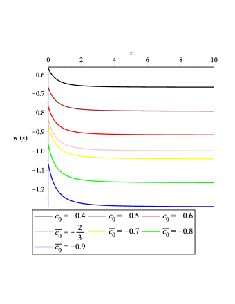
Figure 1: EoS given by Eq. (14) as a function of the redshift for some values of $\bar{c_{0}}$.

It is worth mentioning that for $z\geq 0$, including both the past and present state of universe, $w(z)$ is always negative for $c_{0}=-\frac{4}{6}$. Therefore, one may use $w(z)$ to describe the primary inflationary and current accelerating expansions of universe. As an example, for $-\frac{5}{6}\leq\bar{c_{0}}\leq-\frac{1}{2}$, EoS is within the $-1\leq\omega(z)\leq-\frac{2}{3}$ range in the $z\rightarrow 0$ limit. Since $\bar{c_{0}}=c_{0}\rho_{x0}$, one can finally has the $\frac{3}{4}\leq\rho_{x0}\leq\frac{5}{4}$ range for $\rho_{x0}$ in this situation. The $\bar{c_{0}}=-\frac{2}{3}$ case leads to interesting behavior. For this case, $w(z)$ tends to $-1$ and $-\frac{5}{6}$ as $z\rightarrow\infty$ and $z\rightarrow 0$, respectively. Therefore, this case may be used to model the dominated fluids in both the primary inflationary and current accelerating phases into one model.

The Friedmann’s equation (4) in the presence of the fluid given by Eq. (13) is written as

$$\frac{H^{2}(z)}{H^{2}_{0}}=\Omega_{m0}(1+z)^{3}+\Omega_{x0}\frac{5(1+z)^{\frac{5}{2}}}{1-6c_{0}(1+z)^{\frac{5}{2}}},$$ (15)

where, taking $H(z=0)=H_{0}$, we have the constraints $\Omega_{x0}=1-\Omega_{m0}$.

Since the deceleration parameter defined as,

$$q=-1-\frac{dH}{da}\frac{a}{H},$$

using Eq. (15) and inserting $c_{0}=-\frac{4}{6}$ we find

$$q(z)=\frac{\frac{5(1-\Omega_{m0})[1-16(1+z)^{\frac{5}{2}}]}{\Omega_{m0}(1+z)^{\frac{1}{2}}}+2[1+4(1+z)^{\frac{5}{2}}]^{2}}{\frac{20(1-\Omega_{m0})[1+4(1+z)^{\frac{5}{2}}]}{\Omega_{m0}(1+z)^{\frac{1}{2}}}+4[1+4(1+z)^{\frac{5}{2}}]^{2}},$$ (16)

which is plotted in Fig. ($2$) for $\Omega_{m0}=0.31$. It tends to $\frac{1}{2}$ and $-0.362$ as $z\rightarrow\infty$ and $z\rightarrow 0$, respectively. Transition to negative deceleration parameters happens around $z\simeq 0.68$ which is close to observation ($z\simeq 0.6$) roos .

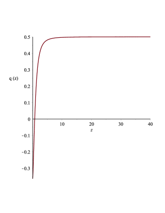
Figure 2: Evolution of the deceleration parameter $q(z)$ defined in Eq. (16). In drawing the graphs we have taken $\Omega_{m0}=0.31$.

The universe can admit a future singularity, if the cosmic fluid satisfies at least one of the below conditions nojp ; od3 :

Type I singularity:

$\rho,|p|\rightarrow\infty$ for $t\rightarrow t_{c}$ and $a\rightarrow\infty$,

Type II singularity:

$\rho\rightarrow\rho_{c}$ and $|p|\rightarrow\infty$, while $t\rightarrow t_{c}$ and $a\rightarrow a_{c}$.

Type III singularity:

$\rho,|p|\rightarrow\infty$, for $t\rightarrow t_{c}$ and $a\rightarrow a_{c}$,

Type IV singularity:

$\rho,|p|\rightarrow 0$, for $t\rightarrow t_{c}$ and $a\rightarrow a_{c}$,

where $t_{c}$, $\rho_{c}$ and $a_{c}\neq 0$ are constant. A phantom source leads to the type I singularity called Big Rip bigrip . The second type, called sudden, happens while $p$ diverges at finite $\rho$, $a$ and thus time sudden . The third type will happen whenever both $\rho$ and $p$ diverge at finite $a$ and thus a finite time od2 . Type IV singularity may also be reached while both $\rho$ and $p$ vanish at finite time and thus a finite scale factor $a$ nojp . The last two types may be appeared in a universe supported by a source with $p=-\rho-f(\rho)$ equation of state nojp ; od2 ; od3 . It is easy to check that Eq. (13) avoids any future singularity for $c_{0}<0$, that means the $c_{0}=-\frac{4}{6}$ case is free from singularity.

III.2 The general proposal for energy and its consequences

Now, bearing the homogeneity and isotropy of the universe in mind, we may write the energy content of the universe as $E=\beta\rho V+\zeta pV$, which is in fact a generalization of the mentioned energy definitions. It covers the Misner-Sharp in the $\zeta=0$ and $\beta=1$ limits. Moreover, it converges to the Komar mass by inserting the $1$ and $3$ values for $\beta$ and $\zeta$ parameters, respectively. Another interesting case is the $\beta=-\zeta=\frac{1}{2}$ case leading to $E=WV$, where $W=\frac{\rho-p}{2}$ is the work density caiwork . The latter case is interesting since it includes the work density which plays the role of pressure in deriving the Friedmann equations by applying the unified first law of thermodynamics on the various horizons of FLRW universe Hay22 ; Hay2 ; Bak ; caiwork ; sheyw1 ; sheyw2 ; ufl ; md .

Following the above recipe for $E=\beta\rho V+\zeta pV$, we obtain that

$$\frac{dp}{d\rho}-\frac{3(\zeta+1)p}{2\zeta\rho}-\frac{\beta}{2\zeta}=0,$$ (17)

which leads to

$$p(\rho)=A\rho^{\frac{3(\zeta+1)}{2\zeta}}-\frac{\beta\rho}{\zeta+3},$$ (18)

where $A$ is an integration constant. Now, inserting the latter equation into (5), we reach

$$\rho(a)=\rho_{x0}[\frac{(\zeta+3-\beta)a^{-\frac{3(\zeta+3-\beta)}{2\zeta}}}{1-A(3+\zeta)a^{-\frac{3(\zeta+3-\beta)}{2\zeta}}}]^{\frac{2\zeta}{3+\zeta}}.$$ (19)

Moreover, for the state parameter and the Friedmann equation in the presence of such fluid, we have

$$w(z)=\bar{A_{1}}[\frac{(\zeta+3-\beta)(1+z)^{\frac{3(\zeta+3-\beta)}{2\zeta}}}{1-A(3+\zeta)(1+z)^{\frac{3(\zeta+3-\beta)}{2\zeta}}}]-\frac{\beta}{\zeta+3},$$ (20)

where $\bar{A_{1}}=A\rho_{x0}^{\frac{\zeta+3}{2\zeta}}$, and

$$\frac{H^{2}(z)}{H^{2}_{0}} =\Omega_{m0}(1+z)^{3}+$$ (21)

$$\Omega_{x0}(\frac{(\zeta+3-\beta)(1+z)^{\frac{3(\zeta+3-\beta)}{2\zeta}}}{1-(\beta-\zeta-2)(1+z)^{\frac{3(\zeta+3-\beta)}{2\zeta}}})^{\frac{2\zeta}{3+\zeta}},$$

respectively. To obtain the last equation, we have considered $A=\frac{\beta-\zeta-2}{3+\zeta}$ which comes from the $\rho(z=0)=\rho_{x0}$ assumption. Calculations for the deceleration parameter lead to

$$q(z)=\frac{1+A(z)}{2(1+B(z))},$$ (22)

in which

$$A(z)$$

$$= \frac{\Omega_{x0}(\zeta+3-\beta)^{\frac{2\zeta}{3+\zeta}}(1+z)^{\frac{3(\zeta+3-\beta)}{3+\zeta}}}{\Omega_{m0}(1+z)^{3}\Big{[}1-(\beta-\zeta-2)(1+z)^{\frac{3(\zeta+3-\beta)}{2\zeta}}\Big{]}^{\frac{3(\zeta+1)}{3+\zeta}}}$$

$$\times [2(\beta-\zeta-2)(1+z)^{\frac{3(\zeta+3-\beta)}{2\zeta}}+\frac{\zeta-3\beta+3}{3+\zeta}]$$

$$B(z)$$

$$= \frac{\Omega_{x0}(\zeta+3-\beta)^{\frac{2\zeta}{3+\zeta}}(1+z)^{\frac{3(\zeta+3-\beta)}{3+\zeta}}}{\Omega_{m0}(1+z)^{3}\Big{[}1-(\beta-\zeta-2)(1+z)^{\frac{3(\zeta+3-\beta)}{2\zeta}}\Big{]}^{\frac{2\zeta}{3+\zeta}}}.$$

It is easy to check that, as a desired result, the previous results are obtainable by inserting $\beta=1$ and $\zeta=3$ into the above equations.

This solution my cover the Polytropic and modified Polytropic models with the Polytropic index $n=\frac{2\zeta}{3+\zeta}$ for $\beta=0$ and $\beta\neq 0$, respectively poly1 . The Chaplygin and modified Chaplygin models with the Chaplygin parameter $\alpha=-\frac{3(\zeta+1)}{2\zeta}$ may also be obtained for $\beta=0$ and $\beta\neq 0$, respectively chap1 ; chap10 . Here, it is worth mentioning that, for $\beta=\zeta+1$, the preceding equation of state converges to a model which was initially introduced in od1 and studied in more details in od2 ; nojp ; od3 . More studies on the various properties of this equation of state, such as its future singularities etc., can be found in od2 ; nojp ; od3 ; jenk ; jenk1 ; nucl . Therefore, our work may give us the energy content of their model and a thermodynamic motivation for that. It is also useful to mention here that the quark bag model quark permits the same relation as Eq. (18), which leads to the obeyance of the results in the cosmological set-ups nucl ; jenk , and therefore, our scheme can be considered as a thermodynamic motivations for their claims and equations of state. In addition, our work gives us the energy content of a universe filled by such component. It is also interesting to mention here that the authors in jenk have considered a fluid with pressure $p=\rho(a-f(\rho))$, while $-1<a$, and study its cosmological applications. They find out that the $f(\rho)\sim\rho^{\mu}$ case, while $\mu>0$, may lead to compatible results with the universe history and its current phase jenk . Let us compare our results with those of Ref. jenk a little more. Comparing their result ($\mu>0$) with Eq. (18), we have obtained that $\frac{\zeta+1}{\zeta}>0$ condition.

Therefore, by this scheme, we found the equation of state for the cosmic fluid with $T^{\mu}_{\nu}=diag(-\rho,p,p,p)$, filling the background, and its corresponding energy in a compatible way with the thermodynamic pressure, Friedmann, continuity, and Raychaudhuri equations. Finally, we should mention our investigation shows that models proposed in od2 ; nojp ; od3 ; jenk ; jenk1 ; nucl can satisfy the Friedmann and thermodynamic equations simultaneously. In Fig. ($3$), $w(z)$ has been plotted for the some values of $\beta$, $\zeta$ and $\bar{A_{1}}$ while $A=\frac{\beta-\zeta-2}{3+\zeta}$. In fact, since we need a fluid of $\omega\leq-\frac{2}{3}$ to model the current phase of universe roos ; mr , we should have $\bar{A_{1}}-\frac{\beta}{\zeta+3}\leq-\frac{2}{3}$ at $z=0$.

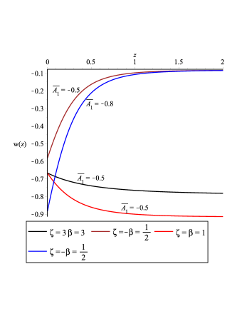
Figure 3: EoS given by Eq. (20) as a function of the redshift for some values of $\beta$, $\zeta$ and $\bar{A}_{1}$.

It is worth mentioning that, in the $z\rightarrow\infty$ limit, $w(z)$ converges to $-\frac{\beta}{\zeta+3}$ while $\frac{3(\zeta+3-\beta)}{2\zeta}\leq 0$, and converges to $\bar{A_{1}}(\frac{\zeta+3-\beta}{\zeta+2-\beta})-\frac{\beta}{\zeta+3}$ if $\frac{3(\zeta+3-\beta)}{2\zeta}\geq 0$. Moreover, as it is clear from Fig ($3$), the $\zeta=3\beta=3$ and $\zeta=\beta=1$ cases, whenever $\bar{A}_{1}=-0.5$, may be used to unify the dominated fluids in both the primary inflationary and current accelerating phases into one model.

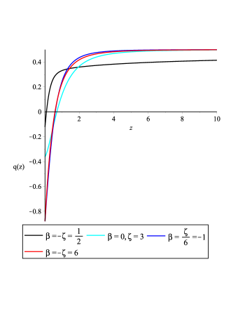
Figure 4: Evolution of the deceleration parameter, Eq. (22), as a function of the redshift.

$q(z)$ has also been plotted in Fig. ($4$) for some values of $\zeta$ and $\beta$, whenever $\Omega_{m0}=0.31$. All the curves converge to $\frac{1}{2}$ at the $z\rightarrow\infty$ limit. Transition from the decelerating universe to an accelerating universe happens around $z\simeq 0.6$ for the $\beta=\frac{\zeta}{6}=-1$ case. Besides, such transition is happen around $z\sim 0.62$ and $z\sim 0.69$ for the $\beta=-\zeta=6$ and ($\beta=0,\zeta=3$) cases, respectively. Finally, it is useful to mention that this transition also happens around $z\sim 0.082$ for the $\beta=-\zeta=\frac{1}{2}$ case.

IV From the equation of state, Friedmann equation and thermodynamic pressure to energy

As we have mentioned in the introduction, the study of the cosmological features of fluids of $p=p(\rho)$ is important prd0 ; capa ; wang . Therefore, we here consider a case in which the $p(\rho)$ relation is given, such as the Polytropic and Chaplygin models. One can use Eq. (6) to obtain $p(V)$. In addition, by inserting the result into Eq. (9) and using Eq. (4) one can obtain an expression for the energy as a function of $\rho$ and $V$. As an example, if we assume that $p=\omega\rho$ and combine Eqs. (4) and (9) with each other, we have that $E=-3\omega\rho V$ relation for energy, as we have previously obtained in the second section, while $\omega$ is constant. Therefore, solutions with $\omega\leq 0$ leads to positive energy, a result which may be in line with the current accelerating universe. However, it is in direct conflict with the radiation and matter dominated eras as well as the thermodynamic stability conditions rafael . One can check to see that the $\rho(a)$ and $a(t)$ relations are the same as those of the standard cosmology. It is also useful to note that the authors in rafael , considered the total mass definition for energy ($E=\rho V$) and they had shown that a dark energy fluid satisfying $p=\omega\rho$, which has only one free parameter including $\omega$, is unphysical. In addition, following the above recipe for $p=K\rho^{\gamma}$ when $K$ and $\gamma$ are constant. We have

$$E=\Big{[}\frac{3}{2\gamma-3}\Big{]}\Big{(}\frac{3}{32\pi}\Big{)}^{\gamma-1}K(\rho V)^{3-2\gamma}$$

for the energy which, as a check, covers the $p=\omega\rho$ case in the appropriate limit $\gamma=1$ and $K=\omega$. The $E>0$ condition also leads to $\gamma>\frac{3}{2}$ for $K>0$ and $\gamma<\frac{3}{2}$ for $K<0$. Here, it is useful to note that these solutions, which have two free parameters including $K$ and $\gamma$, may satisfy the thermodynamic stability conditions abri ; plb1 ; plb2 ; ptp .

Let us now consider the general case $p=K\rho^{\gamma}$ and insert it into Eq. (5) to obtain

$$\rho(a)=\rho_{0}\Big{[}a^{3(\gamma-1)}-K\Big{]}^{\frac{1}{1-\gamma}},$$ (24)

for density. By using Eq. (6), we can write that

$$V(a)=V_{0}\Big{[}a^{3(\gamma-1)}-K\Big{]}^{\frac{3}{2(\gamma-1)}},$$ (25)

where $V_{0}=2(\frac{32\pi}{3})^{-\frac{1}{2}}\rho_{0}^{-\frac{3}{2}}$. We can see that for $\frac{3}{2}<\gamma$, density and volume are decreased and increased, respectively. Now, let us study the behavior of the deceleration factor $q=-1-\frac{\dot{H}}{H^{2}}$. Since $1+z=\frac{1}{a}$, where $z$ is the redshift, by using Eqs. (4), (8) and (24) we can write that

$$q=\frac{1}{2}[1+\frac{K^{\prime}(1+z)^{3(\gamma-1)}}{1-K(1+z)^{3(\gamma-1)}}],$$ (26)

where $K^{\prime}=3K\rho_{0}^{\gamma-1}$. For $\gamma>\frac{3}{2}$, while $E>0$, we reach

$$q\sim\frac{1}{2}\Big{[}1-\frac{K^{\prime}}{K}\Big{]},$$ (27)

and

$$q\sim\frac{1}{2}\Big{[}1+\frac{K^{\prime}}{1-K}\Big{]},$$ (28)

for the $z\rightarrow\infty$ and $z\rightarrow 0$ limits, respectively. Bearing the deceleration parameter of radiation matter era ($q=1$) in mind, by implying this condition to Eq. (27) we have $\rho_{0}=(\frac{-1}{3})^{\frac{1}{\gamma-1}}$. In order to have an estimation for $K$, we insert the $q=-0.6$ value for the $z\rightarrow 0$ limit roos , leading to $K=\frac{11}{16}$, which is compatible with the $E>0$ and $\gamma>\frac{3}{2}$ conditions, and thus $K^{\prime}=-\frac{11}{16}$. Finally, we have

$$q=\frac{1}{2}\Big{[}1-\frac{11(1+z)^{3(\gamma-1)}}{16-11(1+z)^{3(\gamma-1)}}\Big{]},$$ (29)

where $\frac{3}{2}<\gamma$. Recent observations indicate that there is a transition from deceleration to acceleration phase at $z\simeq 0.6$ in the universe history obs1 ; obs2 ; obs3 . Using this observational result in Eq. (29) we have that $\gamma\simeq 0.77$ which is in contrast with $\frac{3}{2}<\gamma$ and thus the $E>0$ expectation. In addition, one can check to see that the $q(z\rightarrow\infty)\rightarrow-1$ initial condition, leads to $K<0$ for $\gamma>\frac{3}{2}$ which is unsatisfactory. Moreover, by applying the $q(z\rightarrow\infty)\rightarrow\frac{1}{2}$ initial condition leads to two solutions. One of them yields $K=0$ which covers the matter dominated era ($q=\frac{1}{2}$ and $\rho(a)=\rho_{0}a^{-3}$) but with $E=0$. The other leads to the unphysical solution $\rho(a)=0$. Therefore, these type of solutions ($\frac{3}{2}<\gamma$) seem unsatisfactory.

Now, let us focus on the $\gamma<\frac{3}{2}$ case, where the $E>0$ condition requires that $K$ should be a negative quantity. For $z\rightarrow\infty$, we can write that $q\simeq\frac{1}{2}$, which signals us to a matter dominated era roos . In order to continue our investigation, we confine ourselves to the $\rho_{0}=1$ case yielding $K^{\prime}=3K$. Additionally, since $q(z\rightarrow 0)\simeq-0.6$ roos and $q(z\simeq 0.6)\simeq 0$ obs1 ; obs2 ; obs3 , we have $K=\frac{K^{\prime}}{3}=-\frac{11}{4}$ and $\gamma\simeq-0.21$. Therefore, a solution with $\rho_{0}=1$, $K=-\frac{11}{4}$ and $\gamma\simeq-0.21$ can satisfy both the theoretical ($E>0$) and observational ($q(z\rightarrow 0)\simeq-0.6$ and $q(z\simeq 0.6)\simeq 0$) conditions. Moreover, simple calculations show that this model is free from any future singularity. Finally, as it is shown in Fig ($4$), this fluid may be used to describe the universe history from the matter dominated era to its current phase.

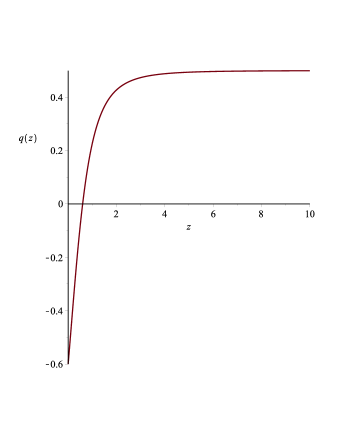
Figure 5: Evolution of the $q(z)$ function.

Moreover, since $E\sim(\rho V)^{3-2\gamma}\sim V^{\frac{3-2\gamma}{3}}$, by simple calculations we obtain $E\sim\frac{1}{((1+z)^{3.63}+\frac{11}{4})^{1.41}}$, for the energy evolution in this model. In order to have a vision about the energy changes in this model, we have plotted $E=E_{0}\frac{1}{((1+z)^{3.63}+\frac{11}{4})^{1.41}}$ for $E_{0}=1$, in Fig ($5$).

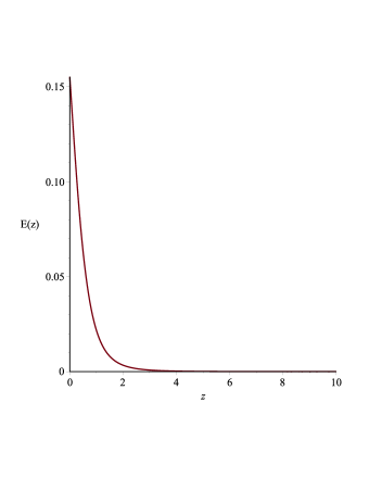
Figure 6: Energy, $E(z)$, of the polytropic gas as a function of the redshift.

However, since $E\rightarrow 0$ in the $z\rightarrow\infty$ limit, it seems that this solution is unsatisfactory for describing the matter dominated era, where $q=\frac{1}{2}$. Therefore, this type of solution may be used to describe a universe with $q<\frac{1}{2}$.

V Observation constraints

In this section we discuss the observational constraints on the cosmological fluid defined in the last section, i.e., the density energy given by Eq. (24). Let us assume that this fluid can be interpreted with a model of unification in the dark sector, i.e, cosmological scenario that unifies dark matter and dark energy. Such proposal has been considered by many authors in the literature chap1 ; chap10 ; DE ; DE0 ; DE1 ; DE2 ; DE3 ; DE4 ; DE5 ; DE6 ; DE7 ; DE8 ; DE9 ; DE10 ; DE11 ; DE12 ; DE13 ; DE14 . Thus, with these considerations the Hubble expansion rate can be written as

$$H(z)$$ (30)

$$\!\!\!\!\!=H_{0}\sqrt{\Omega_{b0}(1+z)^{3}+(1-\Omega_{b0})[(1+z)^{-3(\gamma-1)}-K]^{\frac{1}{1-\gamma}}}$$

To fit the free parameters $K$, $\lambda$, and $h$, we can use the public code CLASS class in connection to the Monte Carlo code public Monte Python monte . We choose the Metropolis Hastings algorithm as our sampling method. The data set utilized in our analysis are: a) Type Ia supernovae (SNe Ia) from Union 2.1 compilation u21 , available at http://supernova.lbl.gov/Union, that contains 580 SN Ia data in the redshift range $0.015\leq z\leq 1.41$; b) Baryon acoustic oscillations (BAO) data measurement from the Six Degree Field Galaxy Survey bao1 , the Main Galaxy Sample of Data Release 7 of Sloan Digital Sky Survey bao2 , the LOWZ and CMASS galaxy samples of the Baryon Oscillation Spectroscopic Survey bao3 , and the distribution of the Lyman Forest in BOSS bao4 ; c) Observational Hubble parameter (OHD) data compiled by X. L Meng et al. hdata , which comprising in 37 data points in the in the redshift range $0.0708\leq z\leq 2.36$. During the realization of statistical analysis we consider $\Omega_{b0}=0.05$ and $|K|$.

Figure 7 shows the confidence regions at 1$\sigma$ and 2$\sigma$ C. L in the plane $\gamma-K$ for the proposed cosmological model. Figure 8 shows the marginalized one-dimensional posterior distribution for the parameters of the models, with their corresponding 1$\sigma$ uncertainties. It is easy to see that for $\gamma=0$ the Hubble expansion rate defined in Eq. (30) has a similar dynamic to the $\Lambda$CDM model, if we assume that $1-\Omega_{b0}\simeq 1$. In this case the constant $K$ plays the role of a “cosmological constant”. Our results summarized in Figures 7 and 8 show that a polytropic gas with EoS given by $p=K\rho^{\gamma}$ has a obvervacional fit compatible with the $\Lambda$CDM model. Showing that a cosmological unified scenario for dark matter and dark energy, and which satisfies the thermodynamic conditions presented in the present work, can fit the current astrophysicists data in the presence of a single dark fluid.

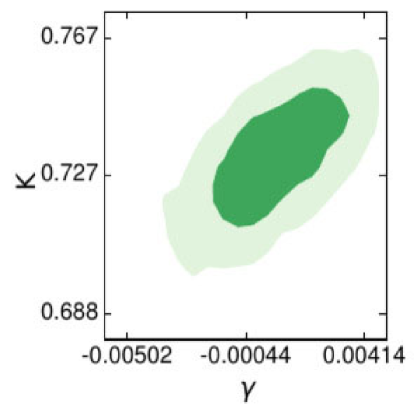
Figure 7: 1$\sigma$ and 2$\sigma$ confidence level in the parametric space $\gamma-K$ from the joint analysis SNe Ia + BAO + OHD.

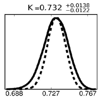
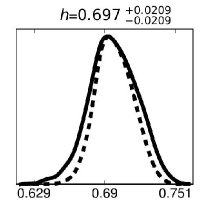
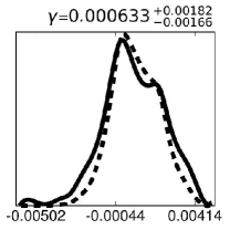
Figure 8: Marginalized one-dimensional posterior distribution for the parameters $K$, $h$, and $\gamma$. The dashed line stands for the average likelihood distribution.

VI Summary and discussion

In the standard cosmology, a perfect fluid with $p=w\rho$ and a constant equation of state ($w$), satisfying the Friedmann and continuity equations simultaneously, can be used to construct a model for the universe expansion. Our analysis shows that, during the cosmos evolution, it is impossible to preserve the Friedmann and the thermodynamic pressure equations simultaneously, if one takes into account the perfect fluid concept. In addition, we have referred to the Komar mass and found that if we combine it with the Friedmann first equation and insert the result into the thermodynamic pressure equation, we construct an equation of state which is similar to the modified polytropic and modified Chaplygin models. Following that, by using the continuity equation, we can write a relation for the density profile of cosmic fluid which may be in agreement with the primary inflationary and current phases of the universe expansion. In fact, the obtained density is free from singularity and it may unify the nature of the dominated fluid in both the primary inflationary and current accelerating eras into one fluid. Moreover, we have considered a special expression for energy that covers the previous definitions. Combining this energy definition with the thermodynamic pressure definition and the Friedmann second equation, we got the $p(V)$ relation. Bearing the Friedmann first equation in mind, we could obtain the $p(\rho)$ relation, and showed that the obtained solutions can be used to model the universe expansion, a result which is in agreement with some previous attempts od1 ; nojp ; od2 ; od3 ; poly1 ; ref57 ; nK ; poly2 ; poly20 ; poly200 ; chap1 ; chap10 ; chap2 ; chap3 ; van ; jenk ; jenk1 ; nucl . We also found out that some type of the obtained solutions may be used to unify the dominated fluids in both the primary inflationary and current accelerating phases into one model. In addition, our study helps us to obtain the corresponding energy of these models, in the cosmological setup, in a similar line with the thermodynamic pressure definition. Therefore, our investigation may also be considered as the thermodynamic motivation for these models. Thereinafter, we have focused on the situation in which the $p(\rho)$ relation is valid. By combining the equation of state with the Friedmann first equation and inserting the result into the pressure thermodynamic definition, we could obtain a relation concerning the energy. Our study shows that this recipe does not lead to a suitable result for the perfect fluid ($p=w\rho$) case. In addition, we saw that the $p=K\rho^{\gamma}$ case, in which $K$ is constant, leads to a solution which may be free from any future singularity and also may govern the universe expansion during the time that its deceleration parameter meets the $q<\frac{1}{2}$ condition. We have constrained the parameters $K$ and $\gamma$ with recent observational data from SNe Ia + BAO + OHD. Based on our results, solving the Friedmann and the thermodynamic pressure equations simultaneously, one gets solutions for cosmic fluids that can be used to model the dark energy candidates. Finally, it is worthwhile mentioning that our investigation suggests that the thermodynamic pressure equation, as a thermodynamic equation of state, imposes serious constraints on the cosmic fluids (solutions of the Friedmann equations), their energy and thus the energy definitions. Therefore, this is still an unanswered question dealing with what kind of fluids and energy definition one can solve the Friedmann and thermodynamics equations simultaneously. The latter being due to the fact that we do not exactly know the true final forms of the laws governing the universe expansion and energy definition in the gravitational theories. We also think one may use the thermodynamic pressure definition to write a relation for the energy of cosmic fluid in the cosmological setups.

References

- (1) M. Roos, Introduction to Cosmology (John Wiley and Sons, UK, 2003).
- (2) H. Moradpour, N. Riazi, Int. J. Theo. Phys. 55, 268 (2016).
- (3) E. M. Barboza, Jr, R. C. Nunes, E. M. C. Abreu, J. A. Neto, Phys. Rev. D 92, 083526 (2015), arXiv:1501.03491 [gr-qc].
- (4) H. Moradpour, A. Sheykhi, N. Riazi, B. Wang, AHEP. 2014, 718583 (2014).
- (5) N. Radicella, D. Pavón, Phys. Lett. B 09, 031 (2011).
- (6) N. Radicella, D. Pavón, Gen. Relativ. Grav. 44, 685 (2012).
- (7) S. Nojiri, S. D. Odintsov, Phys. Rev. D 70, 103522 (2004).
- (8) S. Nojiri, S. D. Odintsov, S. Tsujikawa, Phys. Rev. D 71, 063004 (2005).
- (9) H. Štefančić, Phys. Rev. D 71, 084024 (2005).
- (10) S. Nojiri, S. D. Odintsov, Phys. Rev. D 72, 023003 (2005).
- (11) U. Mukhopadhyay, S. Ray, Mod. Phys. Lett. A 23, 3198 (2008).
- (12) M. Malekjani, Int. J. Theor. Phys. 52, 2674 (2013).
- (13) S. Asadzadeh. Z. Safari, K. Karami, A. Abdolmaleki, Int. J. Theor. Phys. 53, 1248 (2014).
- (14) P. H. Chavanis, arXiv:1208.1185.
- (15) P. H. Chavanis, Eur. Phys. J. Plus, 129, 222 (2014).
- (16) P. H. Chavanis,Eur. Phys. J. Plus. 129, 38 (2014).
- (17) A. Kamenshchik, U. Moschella, V. Pasquier, Phys. Lett. B 511, 265 (2001)
- (18) M. C. Bento, O. Bertolami, A. A. Sen, Phys. Rev. D 66, 043507 (2002).
- (19) H. B. Benaoum, hep-th/0205140.
- (20) E. O. Kahya, B. Pourhassan, Mod. Phys. Lett. A 30, 1550070 (2015).
- (21) R. C. S. Jantsch, M. H. B. Christmann, G. M. Kremer, Int. J. Mod. Phys. D. DOI: 10.1142/S0218271816500310.
- (22) L. L. Jenkovszky, V. I. Zhdanov, E.J. Stukalo, Phys. Rev. D 90, 023529 (2014).
- (23) L. Jenkovszky, B. K mpfer, V. Sysoev, Z. Phys. C 48, 147 (1990).
- (24) S. M. Sanches Jr., F. S. Navarra, D. A. Foga a, Nucl. Phys. A 937, 1 (2015).
- (25) L. Jenkovszky, A. A. Trushevsky, Nuovo. Cimento. Soc. Ital. Fis. A 34, 369 (1976).
- (26) Alfredo B. Henriques, R. Potting, Paulo M. Sá, Phys. Rev. D 79, 103522 (2009).
- (27) K. Bamba, S. Capozziello, S. Nojiri, and S. D. Odintsov, Astrophys. Space. Sci. 342, 155 (2012).
- (28) B. Wang, E. Abdalla, F. Atrio-Barandela, D. Pavon, arXiv:1603.08299v2.
- (29) F. C. Santos, M. L. Bedran, V. Soares, Phys. Lett. B 636, 86 (2006).
- (30) F. C. Santos, M. L. Bedran, V. Soares, Phys. Lett. B 646, 215 (2007).
- (31) M. L. Bedran, V. Soares, Prog. Theor. Phys. 123, 1 (2010).
- (32) H. Moradpour, A. Abri, H. Ebadi, Int. J. Mod. Phys. D 25, 1650014 (2016).
- (33) C. M. Misner, D. H. Sharp, Phys. Rev. B 136, 571 (1964).
- (34) S. A. Hayward, Class. Quantum Grav. 15, 3147 (1998).
- (35) S. A. Hayward, S. Mukohyana, M. C. Ashworth, Phys. Lett. A 256, 347 (1999).
- (36) D. Bak, S. J. Rey, Class. Quantum Grav. 17, L83 (2000).
- (37) R. G. Cai, S. P. Kim, JHEP 0502, 050 (2005).
- (38) A. Sheykhi, B. Wang, R. G. Cai, Nucl. Phys. B 779, 1 (2007).
- (39) A. Sheykhi, B. Wang, R. G. Cai, Phys. Rev. D 76, 023515 (2007).
- (40) D. W. Tian, I. Booth, Phys. Rev. D 92, 024001 (2015).
- (41) H. Moradpour, R. Dehghani, AHEP. 2016, 7248520 (2016).
- (42) E. Verlinde, JHEP 1104, 029 (2011).
- (43) A. Sheykhi, H. Moradpour, N. Riazi, Gen. Rel. Grav. 45, 1033 (2013).
- (44) H. Moradpour, A. Sheykhi, Int. J. Theo. Phys. 55, 1145 (2016).
- (45) T. Padmanabhan. arXiv:1206.4916 (2012).
- (46) R. G. Cai, L. M. Cao, N. Ohta, Phys. Rev. D 81, 061501(R) (2010).
- (47) H. Moradpour, Int. J. Theo. Phys. DOI: 10.1007/s10773-016-3043-6 (2016).
- (48) S. A. Hayward, Phys. Rev. D 49, 831 (1994).
- (49) H. B. Callen, Thermodynamics and Introduction to Thermostatics (New York: John Wiley and Sons, 1985).
- (50) R. K. Pathria, Statistical Mechanics (Linacre House: Oxford OX2 8DP, 1996).
- (51) O. Luongo, H. Quevedo, Int. J. Mod. Phys. D 23, 1450012 (2014).
- (52) G. F. Ellis, R. R. Maartens, M. A. H. MacCallum. Relativistic Cosmology (Cambridge: Cambridge UP, 2012).
- (53) J. D. Barrow, Class. Quant. Grav. 21, L79 (2004).
- (54) R. A. Daly et al., Astrophys. J. 677, 1 (2008).
- (55) WMAP Collab. (E. Komatsu et al.), Astrophys. J. Suppl. 192, 18 (2011).
- (56) V. Salvatelli, A. Marchini, L. L. Honorez, O. Mena, Phys. Rev. D 88, 023531 (2013).
- (57) N. Bilic, G. B. Tupper and R. D. Viollier, Phys. Lett. B, 35, 17 (2002).
- (58) T. Padmanabhan and T. Roy Choudhury, Phys. Rev. D, 66, 081301 (2002).
- (59) M. Susperregi, Phys. Rev. D, 68, 123509 (2003).
- (60) V. F. Cardone, A. Troisi and S. Cappozziello, Phys. Rev. D, 69, 083517 (2004).
- (61) R. J. Scherrer, Phys. Rev. Lett., 93, 011301 (2004).
- (62) R. Mainini, L. P. L. Colombo, S. A. Bonometto, Astrophys. J, 632, 691 (2005).
- (63) D. Giannakis and W. Hu, Phys. Rev. D, 72, 063502 (2005).
- (64) N. Bose and A. S. Majumdar, Phys. Rev. D, 80, 103508 (2009).
- (65) C. Gao, M. Kunz and A. R. Liddle, Phys. Rev. D, 81, 043520, (2010).
- (66) D. Bertacca, N. Bertolo and S. Matarrese, Adv. Astron., 2010, 904379 (2010).
- (67) H. Sandvik, M. Tegmark, M Zaldarriaga and I. Waga, Phys. Rev. D, 69, 123524 (2004).
- (68) L. M. G. Beca, P. P. Avelino, J. P. M. de Carvalho and C. J. A. P. Martins, Phys. Rev. D, 67, 101301 (2003).
- (69) R. R. R. Reis, I. Waga, M. O. Calvao and S. E. Joras, Phys. Rev. D, 68, 061302 (2003).
- (70) P. P. Avelino, J. P. M. de Carvalho, C. J. A. P. Martins and E. J. Copeland, Phys. Rev. D., 69, 041301 (2004).
- (71) N. Billic, R. J. Lindebaum, G. Tupper and R. Viollier, JCAP, 0411, 008 (2004).
- (72) M. C. Bento, O. Bertolami and A. A. Sen, Phys. Rev. D, 70, 083519 (2004).
- (73) D. Blas, J. Lesgourgues, and T. Tram, The Cosmic Linear Anisotropy Solving System (CLASS). Part II: Approximation schemes,” JCAP 7 34 (2011), arXiv:1104.2933.
- (74) B. Audren, J. Lesgourgues, K. Benabed, and S. Prunet, Conservative constraints on early cosmology with monte python, JCAP 2 1 (2013), arXiv:1210.7183.
- (75) N. Suzuki, et al., [The Supernova Cosmology Project], Astrophys. J. 746, 85 (2012); http://supernova.lbl.gov/Union/.
- (76) F. Beutler, C. Blake, M. Colless, D. H. Jones, L. Staveley-Smith, L. Campbell, Q. Parker, W. Saunders, and F. Watson, MNRAS 416 3017-3032 (2011), arXiv:1106.3366.
- (77) A. J. Ross, L. Samushia, C. Howlett, W. J. Percival, A. Burden, and M. Manera, MNRAS 449 835-847 (2015), arXiv:1409.3242.
- (78) L. Anderson, et al., MNRAS 441 24-62 (2014), arXiv:1312.4877.
- (79) A. Font-Ribera, et al., JCAP 5 27 (2014), arXiv:1311.1767.
- (80) X. L. Meng, X. Wang, S. Li, and T. J. Zhang, arXiv:1507.02517 (2015).