Linear and nonlinear ion-acoustic waves in non-relativistic quantum plasmas with arbitrary degeneracy

Abstract

Linear and nonlinear ion-acoustic waves are studied in a fluid model for non-relativistic, unmagnetized quantum plasma with electrons with an arbitrary degeneracy degree. The equation of state for electrons follows from a local Fermi-Dirac distribution function and apply equally well both to fully degenerate or classical, non-degenerate limits. Ions are assumed to be cold. Quantum diffraction effects through the Bohm potential are also taken into account. A general coupling parameter valid for dilute and dense plasmas is proposed. The linear dispersion relation of the ion-acoustic waves is obtained and the ion-acoustic speed is discussed for the limiting cases of extremely dense or dilute systems. In the long wavelength limit the results agree with quantum kinetic theory. Using the reductive perturbation method, the appropriate Korteweg-de Vries equation for weakly nonlinear solutions is obtained and the corresponding soliton propagation is analyzed. It is found that soliton hump and dip structures are formed depending on the value of the quantum parameter for the degenerate electrons, which affect the phase velocities in the dispersive medium.

I Introduction

The study of degenerate plasma is important due to its applications e.g. to strong laser produced plasmas r2 , high density astrophysical plasmas such as in white dwarfs or neutron stars r5 , or large density electronic devices (as in the drain region of $n^{+}nn^{+}$ diodes r1 ). In plasmas, the quantum effects are more relevant for electrons rather than ions because of their lower mass. The quantum nature of the charge carriers manifests with the inclusion of both Pauli exclusion principle for fermions and Heisenberg uncertainty principle due to the wave like character of the particles. Accordingly, electrons obey the Fermi-Dirac statistics and their equation of state is determined using the Fermi-Dirac distribution. On the other hand the quantum diffraction effects are usually modeled by means of quantum recoil terms in kinetic theory or the Bohm potential in fluid theory, besides higher order gradient corrections r8 ; mel .

Accordingly, the wave propagation in a degenerate plasma can be studied using at least two main approaches i.e., kinetic and hydrodynamic models. In kinetic theory, the unperturbed electron distribution is frequently given by a Fermi-Dirac function, while in hydrodynamics the momentum equation for electrons is made consistent with the equation of state of a degenerate electron Fermi gas r8 ; mel . In fluid models, the ion-sound wave propagation in plasmas with degenerate electrons has been investigated by a number of authors r12 ; r13 ; r14 ; r15 ; r16 ; r17 ; r18 , using the equation of state for a cold (fully degenerate) Fermi electron gas, with a negligible thermodynamic temperature. The energy distribution of a degenerate electron gas described by the Fermi-Dirac distribution is characterized by independent parameters, one of which is the chemical potential, while the other is the thermodynamic temperature. On the other hand, the energy spread for the classical ideal electron gas obeying Maxwell-Boltzmann distribution is uniquely determined by the thermodynamic temperature. The equation of state for the fully degenerate electron gas so reduces to an one-parameter problem i.e., the chemical potential. Therefore, it is of interest to study the linear and specially nonlinear wave propagation in the intermediate regime, depending on the competition between the two parameters i.e., chemical potential and thermal temperature r11 , including quantum diffraction.

Our treatment is specially relevant to borderline systems with $T\approx T_{F}$, which are neither strongly degenerate nor sufficiently well described by classical statistics, where $T$ and $T_{F}$ are resp. the electron thermodynamic and Fermi temperatures. A striking example is provided by inertial confinement fusion plasmas solid , with particle densities ranging from $10^{30}m^{-3}$ to $10^{32}m^{-3}$, and thermodynamic temperatures above $10^{7}K$. During laser irradiation of the solid target, quantum statistical effects tend to be more relevant immediately after compression, before the heating phase. Moreover, laboratory simulation of astrophysical scenarios involving dense plasmas better fit the intermediate quantum-classical regime gregori . For these reasons and potential applications on e.g. ultra-small semiconductor devices operating in a mixed dense-dilute regime r1 , it is desirable to have a general macroscopic model covering both classical and quantum statistics, besides quantum diffraction.

Previously, Maafa r19 studied the ion-acoustic and Langmuir waves in a plasma with arbitrary degeneracy of electrons using classical kinetic theory, linearizing the Vlasov-Poisson system around a Fermi-Dirac equilibrium. Using quantum kinetic theory, Melrose and Mushtaq derived the electron-ion plasma low-frequency longitudinal response including quantum recoil, first for dilute (Maxwell-Boltzmann equilibrium) plasmas r22 and then mm for general degeneracy, in a Fermi-Dirac equilibrium. These works were restricted to linear waves only. Eliasson and Shukla r23 derived nonlinear quantum electron fluid equations by taking the moments of the evolution equation for the Wigner function in terms of a local Fermi-Dirac equilibrium with an arbitrary thermodynamic temperature. In this model quantum diffraction manifest in terms of the Bohm potential. The high (classical) as well as the low (degenerate) temperature limits of the obtained fluid equations were also discussed in connection to Langmuir waves. Recently Dubinov et al. r24 investigated the nonlinear theory of ion-acoustic waves in isothermal plasmas with arbitrary degeneracy, but without including quantum recoil. They presented the equation of state for ions and electrons by considering them as warm ($T\neq 0$) Fermi gases. The nonlinear analysis was done using a Bernoulli pseudo-potential approach. The ranges of the phase velocities of the periodic ion-acoustic waves and the soliton velocity were investigated. However, for simplicity they ignored the quantum Bohm potential, which increases the order of the resulting dynamical equations. Our central issue here is to analyze the combined quantum statistical and quantum diffraction effects on linear and nonlinear ion-acoustic structures in plasmas, in an analytically simple (but hopefully not simplistic) approach.

The manuscript is organized in the following way. In Section II, the basic set of hydrodynamic equations is proposed and the barotropic equation of state defined, for a general Fermi-Dirac equilibrium. In Section III, the linear dispersion relation for quantum ion-acoustic waves is derived, following the fluid model. Comparison with known results from quantum kinetic theory allows to determine a fitting parameter in the quantum force, so that the macroscopic and microscopic approaches coincide in the long wavelength limit. In Section IV, nonlinear wave structures are studied by means of the reductive perturbation method and the associated Korteweg-de Vries (KdV) equation. The associated quantum soliton solution is obtained. Section V studies the possibility of forward and backward propagating solitons in real systems. Finally, Section VI collect some conclusions.

II Model equations

In order to study ion-acoustic waves in unmagnetized electron-ion plasmas with arbitrary electron temperature, we use the set of dynamic equations described as follows r8 .

The ion continuity and momentum equations are respectively given by

$$\frac{\partial n_{i}}{\partial t}+\frac{\partial}{\partial x}(n_{i}u_{i}) = 0\,,$$ (1)

$$\frac{\partial u_{i}}{\partial t}+u_{i}\frac{\partial u_{i}}{\partial x} = -\frac{e}{m_{i}}\frac{\partial\phi}{\partial x}\,.$$ (2)

The momentum equation for the inertialess quantum electron fluid is given by

$$0=e\frac{\partial\phi}{\partial x}-\frac{1}{n_{e}}\frac{\partial p}{\partial x}+\frac{\alpha\,\hbar^{2}}{6\,m_{e}}\frac{\partial}{\partial x}\left(\frac{1}{\sqrt{n_{e}}}\frac{\partial^{2}}{\partial x^{2}}\sqrt{n_{e}}\right).$$ (3)

The Poisson equation is written as

$$\frac{\partial^{2}\phi}{\partial x^{2}}=\frac{e}{\varepsilon_{0}}(n_{e}-n_{i})\,,$$ (4)

where $\phi$ is the electrostatic potential. The ion fluid density and velocity are represented by $n_{i}$ and $u_{i}$ respectively, while $n_{e}$ is the electron fluid density. Also, $m_{e}$ and $m_{i}$ are the electron and ion masses, $-e$ is the electronic charge, $\varepsilon_{0}$ the vacuum permittivity and $\hbar$ the reduced Planck constant. In Eq. (3), $\alpha$ is a dimensionless constant factor to be determined and $p=p(n_{e})$ is the electron’s fluid scalar pressure, to be specified by a barotropic equation of state obtained in the continuation.

The last term proportional to $\hbar^{2}$ on the right hand side of the momentum equation for electrons is the quantum force, which arises due to the quantum Bohm potential, responsible for quantum diffraction or quantum tunneling effects due to the wave like nature of the electrons. The dimensionless quantity $\alpha$ will be selected in order to exactly fit the kinetic theory linear dispersion relation in a three-dimensional Fermi-Dirac equilibrium, as detailed in Section III. It is known that the qualitative role of the Bohm potential is to provide extra dispersion. However, the precise numerical coefficient in its definition is a debatable subject involving e.g. the dimensionality and the temperature Barker . For instance, for a local Maxwell-Boltzmann equilibrium, Gardner Gardner has found a factor $\alpha=1$. Frequently, the factor $\alpha$ is set in order to fit numerical results from kinetic theory Grubin , which is in the spirit of the present work. On the other hand, quantum effects on ions are ignored in the model in view of their large mass. For simplicity, ion temperature effects are also disregarded.

In order to derive the equation of state, consider a local quasi-equilibrium Fermi-Dirac particle distribution function $f=f(\mathbf{v},\mathbf{r},t)$ for electrons r26 , given by

$$f(\mathbf{v},\mathbf{r},t)=\frac{A}{1+e^{\beta(\varepsilon-\mu)}}\,,$$ (5)

where $\beta=1/(\kappa_{B}T)$, $\varepsilon=m_{e}v^{2}/2,v=|\mathbf{v}|$ and $\mu$ is the chemical potential regarded as a function of position $\mathbf{r}$ and time $t$. Besides, $\kappa_{B}$ is the Boltzmann constant, $T$ is the (constant) thermodynamic electron’s temperature and $\mathbf{v}$ is the velocity. In addition, $A$ is chosen to ensure the normalization $\int\!fd^{3}v=n_{e}$, so that

$$A=-\,\frac{n_{e}}{\mathrm{Li}_{3/2}(-e^{\beta\mu})}\left(\frac{\beta m_{e}}{2\pi}\right)^{3/2}=2\left(\frac{m_{e}}{2\pi\hbar}\right)^{3}\,,$$ (6)

the last equality following from the Pauli principle (the factor two is due to the electron’s spin). Therefore, in the fluid description, $\mu$ and $A$ are supposed to be slowly varying functions of space and time. Equation (6) contains the poly-logarithm function $\mathrm{Li}_{\nu}(\eta)$ of index $\nu$, which can be generically defined r27 by

$$\mathrm{Li}_{\nu}(\eta)=\frac{1}{\Gamma(\nu)}\int_{0}^{\infty}\frac{s^{\nu-1}}{e^{s}/\eta-1}\,ds\,,$$ (7)

where $\Gamma(\nu)$ is the Gamma function. We also observe that a three-dimensional equilibrium is assumed, although for electrostatic wave propagation only one spatial variable $x$ is needed in the model equations.

The scalar pressure follows from the standard definition for an equilibrium with zero drift velocity,

$$p=\frac{m_{e}}{3}\int\!fv^{2}d^{3}v\,,$$ (8)

yielding

$$p=\frac{n_{e}}{\beta}\frac{\mathrm{Li}_{5/2}(-e^{\beta\mu})}{\mathrm{Li}_{3/2}(-e^{\beta\mu})}\,.$$ (9)

It is worth to consider some limiting cases of the barotropic equation of state. From Eq. (9), in the dilute plasma limit case with a local fugacity $e^{\beta\mu}\ll 1$ and using $\mathrm{Li}_{\nu}(-e^{\beta\mu})\approx-e^{\beta\mu}$, one has

$$p=n_{e}k_{B}T\,,$$ (10)

which is the classical isothermal equation of state.

On the opposite, dense limit with a large local fugacity $e^{\beta\mu}\gg 1$, from $\mathrm{Li}_{\nu}(-e^{\beta\mu})\approx-\left(\beta\mu\right)^{\nu}/\Gamma(\nu+1)$ the result is

$$p=\frac{2}{5}\,n_{0}\varepsilon_{F}\,\left(\frac{n_{e}}{n_{0}}\right)^{5/3}\,,$$ (11)

which is the equation of state for a three-dimensional completely degenerate Fermi gas, expressed in terms of the equilibrium number density $n_{0}$. In Eq. (11), the electron’s Fermi energy is $\varepsilon_{F}=\kappa_{B}T_{F}=[\hbar^{2}/(2m_{e})]\,(3\pi^{2}n_{0})^{2/3}$, which is the same as the equilibrium chemical potential in the fully degenerate case. In addition, $n_{0}$ is the equilibrium electron (and ion) number density.

The present treatment has similarities, as well as some different choices, in comparison to Eliasson and Shukla work r23 . In this article, also a local quasi-equilibrium Fermi-Dirac distribution function was employed. However, presently a non-constant chemical potential is admitted. In addition, in Ref. r23 the focus was on situations involving one-dimensional laser-plasma compression experiments, while here it is assumed a three-dimensional isotropic equilibrium. Finally, the present work deals with low-frequency (ion-acoustic) instead of high-frequency (Langmuir) waves.

In passing, from Eq. (6) one deduce the useful relation

$$n_{e}=n_{0}\,\frac{\mathrm{Li}_{3/2}(-e^{\beta\mu})}{\mathrm{Li}_{3/2}(-e^{\beta\mu_{0}})}\,,$$ (12)

where $\mu_{0}$ is the equilibrium chemical potential, satisfying

$$-\,\frac{n_{0}}{\mathrm{Li}_{3/2}(-e^{\beta\mu_{0}})}\left(\frac{\beta m_{e}}{2\pi}\right)^{3/2}=2\left(\frac{m_{e}}{2\pi\hbar}\right)^{3}\,.$$ (13)

Using the equation of state (9), the chain rule and the property $d\mathrm{Li}_{\nu}(\eta)/d\eta=(1/\eta)\mathrm{Li}_{\nu-1}(\eta)$, the momentum equation (3) for the inertialess electron fluid becomes

$$0 = e\frac{\partial\phi}{\partial x}-\frac{1}{\beta n_{e}}\frac{\mathrm{Li}_{3/2}(-e^{\beta\mu})}{\mathrm{Li}_{1/2}(-e^{\beta\mu})}\frac{\partial n_{e}}{\partial x}$$ (14)

$$+ \frac{\alpha\,\hbar^{2}}{6\,m_{e}}\frac{\partial}{\partial x}\left(\frac{1}{\sqrt{n_{e}}}\frac{\partial^{2}}{\partial x^{2}}\sqrt{n_{e}}\right)\,.$$

Finally, using Eq. (12), we have the alternative form

$$0 = e\frac{\partial\phi}{\partial x}-\frac{1}{\beta n_{0}}\frac{\mathrm{Li}_{3/2}(-e^{\beta\mu_{0}})}{\mathrm{Li}_{1/2}(-e^{\beta\mu})}\frac{\partial n_{e}}{\partial x}$$ (15)

$$+ \frac{\alpha\,\hbar^{2}}{6\,m_{e}}\frac{\partial}{\partial x}\left(\frac{1}{\sqrt{n_{e}}}\frac{\partial^{2}}{\partial x^{2}}\sqrt{n_{e}}\right)\,,$$

containing the minimal number of poly-logarithmic functions with a non-constant argument.

It is worth noticing that the model does not include collisional damping, which is reasonable if the average electrostatic potential per particle $\langle U\rangle$ is much smaller than the corresponding average kinetic energy $\langle K\rangle$. For any degree of degeneracy, one can estimate $\langle U\rangle\approx e^{2}/(4\pi\varepsilon_{0}r_{S})$, where the Wigner-Seitz ratio $r_{S}$ is defined by $(4\pi r_{S}^{3}/3)\,n_{0}=1$. On the other hand, from $\langle K\rangle=[m_{e}/(2n_{e})]\int fv^{2}d^{3}v$ and evaluating on equilibrium, one derive the general coupling parameter

$$g \equiv \frac{\langle U\rangle}{\langle K\rangle}=\frac{1}{6}\left(\frac{4}{3\pi^{2}}\right)^{1/3}\frac{e^{2}n_{0}^{1/3}\beta}{\varepsilon_{0}}\frac{\mathrm{Li}_{3/2}(-e^{\beta\mu_{0}})}{\mathrm{Li}_{5/2}(-e^{\beta\mu_{0}})}$$ (16)

$$= -\frac{\sqrt{\beta m_{e}/2}}{3^{4/3}\pi^{7/6}}\,\,\frac{e^{2}}{\varepsilon_{0}\hbar}\frac{(\mathrm{Li}_{3/2}^{2}(-e^{\beta\mu_{0}}))^{2/3}}{\mathrm{Li}_{5/2}(-e^{\beta\mu_{0}})}\,,$$

covering both degenerate and non-degenerate systems, in the non-relativistic regime. In the last equality in Eq. (16) it was used the expression (13) of the equilibrium density in terms of the equilibrium fugacity $z=e^{\beta\mu_{0}}$ and the temperature $T$. In the dilute case, it follows from the properties of the poly-logarithm function that $g\propto\langle U\rangle/(\kappa_{B}T)$, while in the dense case $g\propto\langle U\rangle/\varepsilon_{F}$, with $\mu_{0}\approx\varepsilon_{F}$.

For both dilute or dense plasmas, the condition for low collisionality is that the interaction energy should be small in comparison to the kinetic energy, or $g\ll 1$ Ak . Using Eq. (16), the minimal temperature $T_{m}$ for low collisionality ($g<1$, relaxing the inequality sign) for both dilute and dense regimes follows from

$$\kappa_{B}T>\kappa_{B}T_{m}\equiv\frac{m_{e}}{2\times 3^{8/3}\pi^{7/3}}\left(\frac{e^{2}}{\varepsilon_{0}\hbar}\right)^{2}\left(\frac{\mathrm{Li}_{3/2}^{4/3}(-e^{\beta\mu_{0}})}{\mathrm{Li}_{5/2}(-e^{\beta\mu_{0}})}\right)^{2}\,.$$ (17)

The result is shown in Fig. (1), where $T>T_{m}$ is equivalent to $g<1$. Starting from $z\approx 0$ and increasing the density, larger temperatures are needed for ideality, until reaching $z=9.8,T=8.5\times 10^{4}K$, corresponding to $n_{0}=2.9\times 10^{29}m^{-3}$. For $z>9.8$, smaller temperatures are admitted, due to the Pauli blocking effect inhibiting collisions.

Figure 1: Temperatures for the coupling parameter $g<1$ in Eq. (16) are above the curve, as a function of the fugacity $z=e^{\beta\mu_{0}}$.

For the sake of comparison, instead of

$$\langle K\rangle=\frac{3}{2}\,\kappa_{B}T\,\frac{\mathrm{Li}_{5/2}(-e^{\beta\mu_{0}})}{\mathrm{Li}_{3/2}(-e^{\beta\mu_{0}})}\,,$$ (18)

Zamanian et al. used Zamanian the useful simpler expression

$$\langle K\rangle_{Z}=\frac{3}{2}\kappa_{B}T+\frac{3}{5}\varepsilon_{F}$$ (19)

as a measure of the kinetic energy per particle. More precisely, Ref. Zamanian employed the arithmetic sum of the thermal and Fermi energies, but in Eq. (19) we set some numerical factors to have agreement with the exact form in the dilute and ultra-dense cases where one has resp. $\langle K\rangle\approx 3\,\kappa_{B}T/2$ and $\langle K\rangle\approx 3\,\varepsilon_{F}/5$. In fact, using Eq. (13) expressing the density in terms of the fugacity and the temperature, as well as the expression of the Fermi energy, one find

$$\frac{\langle K\rangle_{Z}}{\kappa_{B}T}=\frac{3}{2}+\frac{3^{5/3}}{10}\left(\frac{\pi}{2}\right)^{1/3}\left[-\mathrm{Li}_{3/2}(-e^{\beta\mu_{0}})\right]^{2/3},$$

where the right-hand sides are functions of the fugacity only. This expression is shown in Fig. (2), compared to the more exact result found from Eq. (18). It is seen that the approximate form overestimates the kinetic energy, due to slow convergence. Nevertheless, by construction, for extreme degeneracy both quantities give the same numbers.

Figure 2: Comparison between the average kinetic energy $\langle K\rangle$ - the continuous curve - given by Eq. (18) and the simpler form $\langle K\rangle_{z}$ - the dashed curve - given by Eq. (19), as a function of the fugacity $z=e^{\beta\mu_{0}}$. Both energies are normalized to $\kappa_{B}T$.

On the same spirit one can define a general electron thermal velocity (in the sense of spreading of velocities) as $v_{T}\equiv\sqrt{2\langle K\rangle/m_{e}}$, which is found from Eq. (18),

$$v_{T}=\left(\frac{3}{\beta m_{e}}\frac{\mathrm{Li}_{5/2}(-e^{\beta\mu_{0}})}{\mathrm{Li}_{3/2}(-e^{\beta\mu_{0}})}\right)^{1/2}\,.$$ (20)

In the dilute case one has $v_{T}\approx\sqrt{3\kappa_{B}T/m_{e}}$, while in the dense case $v_{T}\approx\sqrt{(6/5)\,\varepsilon_{F}/m_{e}}$.

For non-degenerate ions in strongly coupled plasma, the ion crystallization effects r271 ; r272 that appear due to viscoelasticity of the ion fluid in the ion momentum equation and cause damping of the ion-acoustic wave are ignored under the assumptions (in three-dimensional version) $\tau_{m}<<\omega_{pi}$ and $\partial{\bf u}_{i}/\partial t>>(\eta/\rho_{i})\nabla^{2}{\bf u}_{i}$ $+(1/\rho_{i})\left(\zeta+\eta/3\right)\nabla\left(\mathbf{\nabla}\cdot{\bf u}_{i}\right)$, where $\rho_{i}=n_{i}m_{i}$ is the ion mass density, $\tau_{m}$ is the viscoelastic relaxation time or memory function for ions, $\eta$ is the shear and $\zeta$ are the bulk ion viscosity coefficients, respectively.

III Linear Waves

III.1 Fluid theory

We linearize the system given by equations (1)-(15) by considering the first order perturbations (with a subscript 1) relative to the equilibrium, as follows,

$$n_{i} = n_{0}+n_{i1}\,,\quad n_{e}=n_{0}+n_{e1}\,,\quad u_{i}=u_{i1}\,,$$

$$\phi = \phi_{1}\,,\quad\mu=\mu_{0}+\mu_{1}\,.$$ (21)

The dispersion relation is obtained assuming plane wave excitations $\sim\exp[i(kx-\omega t)]$, yielding

$$\omega^{2}=\frac{\omega_{pi}^{2}c_{s}^{2}k^{2}\left(1+\frac{\alpha\,\hbar^{2}k^{2}}{12\,m_{e}m_{i}c_{s}^{2}}\right)}{\omega_{pi}^{2}+\left(1+\frac{\alpha\,\hbar^{2}k^{2}}{12\,m_{e}m_{i}c_{s}^{2}}\right)c_{s}^{2}k^{2}}\,,$$ (22)

where

$$c_{s}=\sqrt{\frac{1}{m_{i}}\left(\frac{\partial p}{\partial n_{e}}\right)_{0}}=\sqrt{\frac{1}{\beta m_{i}}\frac{\mathrm{Li}_{3/2}(-e^{\beta\mu_{0}})}{\mathrm{Li}_{1/2}(-e^{\beta\mu_{0}})}}$$ (23)

plays the role of a generalized ion-acoustic speed and $\omega_{pi}=\sqrt{n_{0}e^{2}/(m_{i}\varepsilon_{0})}$ is the ion plasma frequency.

In the long wavelength limit $\alpha\,\hbar^{2}k^{4}/(12m_{e}m_{i})\ll c_{s}^{2}k^{2}\ll\omega_{pi}^{2}$ it follows from Eq.(22) that $\omega^{2}\approx c_{s}^{2}k^{2}$. In the dilute case with a small fugacity $e^{\beta\mu_{0}}\ll 1$ the well-known classical result $c_{s}\approx c_{sc}\equiv\sqrt{\kappa_{B}T/m_{i}}$ is verified. In the opposite, extremely degenerate case where the fugacity $e^{\beta\mu_{0}}\gg 1$ one find $c_{s}\approx\sqrt{(2/3)\varepsilon_{F}/m_{i}}$, which is the ion-acoustic velocity for a three-dimensional ultra-dense plasma r19 . Finally, the very short wavelength limit of the dispersion relation gives ion oscillations such that $\omega=\omega_{pi}$, both in the classical or quantum situations. This happens because the ions are no longer shielded by electrons when wavelength is comparable to or smaller than the electron shielding length. It is interesting to note that taking the square root of both sides of Eq.(22) is identical to Eq.(4.5) in Ref.r191 for the completely degenerate plasma case i.e., for $\alpha=1/3$.

Using Eq. (23), the ion-acoustic speed $c_{s}$ normalized to the purely classical expression $c_{sc}$ against $z=e^{\beta\mu_{0}}$ is shown in Fig.(3). It can be seen that as the value of $z$ increases (i.e. the degeneracy of electrons and plasma density increase) the ion-acoustic speed also increases.

Figure 3: The profile of the ion-acoustic speed $c_{s}$ from Eq. (23), normalized to the classical expression $c_{sc}$, as a function of the fugacity $z=e^{\beta\mu_{0}}$.

III.2 Kinetic theory

To endorse the macroscopic modeling, and to set the value of the parameter $\alpha$ in front of the quantum force, it is useful to compare with the microscopic (quantum kinetic) results. Considering the Wigner-Poisson system r8 involving a cold ionic species and electrons, it is straightforward to derive the linear dispersion relation

$$1=\frac{\omega_{pi}^{2}}{\omega^{2}}+\frac{\omega_{pe}^{2}}{n_{0}}\int\frac{f_{0}(\mathbf{v})\,d^{3}v}{(\omega-\mathbf{k}\cdot\mathbf{v})^{2}-\hbar^{2}k^{4}/(4m_{e}^{2})}\,,$$ (24)

where $f_{0}(\mathbf{v})$ is the equilibrium electronic Wigner function and $\omega_{pe}=\sqrt{n_{0}e^{2}/(m_{e}\varepsilon_{0})}$ is the electron plasma frequency.

The longitudinal response of an electron-ion plasma in a Fermi-Dirac equilibrium

$$f_{0}(\mathbf{v})=\frac{A}{1+e^{\beta(\varepsilon-\mu_{0})}}$$ (25)

has been calculated in mm , where $A$ and $\mu_{0}$ are obtained from Eq. (13). Including the first order correction from quantum recoil, the result is

$$1=\frac{\omega_{pi}^{2}}{\omega^{2}} - \frac{\omega_{pi}^{2}}{c_{s}^{2}k^{2}}\Bigl{[}1$$

$$- \frac{m_{e}\left(\omega^{2}+\hbar^{2}k^{4}/(12\,m_{e}^{2})\right)}{k^{2}\kappa_{B}T}\,\frac{\mathrm{Li}_{-1/2}(-e^{\beta\mu_{0}})}{\mathrm{Li}_{1/2}(-e^{\beta\mu_{0}})}\Bigr{]}\,,$$

which follows from Eq. (29) of mm , in a different notation. The first and second terms in the right-hand side of Eq.(III.2) are, respectively, the ionic and electronic responses of the plasma.

For the treatment of low-frequency waves, for simplicity it is sufficient to consider the static electronic response, so that we set $\omega\approx 0$ in the last term of Eq. (III.2). From inspection, and since we want to retain the first order quantum correction, this approximation requires $\omega^{2}\ll\hbar^{2}k^{4}/(12\,m_{e}^{2})$. Under the long wavelength assumption $k^{2}c_{s}^{2}\ll\omega_{pi}^{2}$ and the leading order result $\omega^{2}\approx c_{s}^{2}k^{2}$, it follows that

$$\frac{12\,m_{e}^{2}c_{s}^{2}}{\hbar^{2}}\ll k^{2}\ll\frac{\omega_{pi}^{2}}{c_{s}^{2}}\,.$$ (27)

Taking into account the ion-acoustic velocity from Eq. (23), from Eq. (27) one has the necessary condition

$$\frac{\beta^{2}\hbar^{2}\omega_{pi}^{2}}{12}\gg\left(\frac{m_{e}}{m_{i}}\right)^{2}\left(\frac{\mathrm{Li}_{3/2}(-e^{\beta\mu_{0}})}{\mathrm{Li}_{1/2}(-e^{\beta\mu_{0}})}\right)^{2}\,.$$ (28)

The combined low-frequency and long wavelength requirement (28) is more easily worked out in the dilute ($e^{\beta\mu_{0}}\ll 1$) and fully degenerate ($e^{\beta\mu_{0}}\gg 1$) cases. For hydrogen plasma and using the appropriate asymptotic expansions of the poly-logarithm functions, one find $n_{0}/T^{2}\gg 3.5\times 10^{16}\,m^{-3}K^{-2}$ in the non-degenerate situation, and $n_{0}\ll 4.5\times 10^{37}\,m^{-3}$ for very dense systems. It is seen that non-degenerate plasmas satisfy (28) more easily in denser and colder plasmas, while fully degenerate plasmas safely fit the assumptions, except for extreme densities (e.g neutron star), which would deserve a relativistic treatment. Otherwise, there would be the need to retain the full electronic response in Eq.(III.2). As a consequence, a somewhat more involved dispersion relation would be found. In fact, using $n_{0}$ from Eq. (13), it can be shown that the necessary condition (28) is safely attended for all fugacities, as far as $T\ll 10^{9}\,K$, which is reasonable in view of the non-relativistic assumption.

Dropping $\omega$ in the electronic response, Eq. (III.2) considerably simplify, reducing to

$$1=\frac{\omega_{pi}^{2}}{\omega^{2}}-\frac{\omega_{pi}^{2}}{c_{s}^{2}k^{2}}\left(1-\frac{\hbar^{2}k^{2}}{12\,m_{e}\kappa_{B}T}\,\frac{\mathrm{Li}_{-1/2}(-e^{\beta\mu_{0}})}{\mathrm{Li}_{1/2}(-e^{\beta\mu_{0}})}\right)\,.$$ (29)

Solving for the frequency yield

$$\omega^{2}=\frac{\omega_{pi}^{2}c_{s}^{2}k^{2}}{\omega_{pi}^{2}+\left(1-\frac{\beta^{2}\hbar^{2}\omega_{pe}^{2}}{12}\frac{\mathrm{Li}_{-1/2}(-e^{\beta\mu_{0}})}{\mathrm{Li}_{3/2}(-e^{\beta\mu_{0}})}\right)c_{s}^{2}k^{2}}\,.$$ (30)

The expression from kinetic theory is valid for wavelengths larger than the electron shielding length of the system. To make a comparison with the result from fluid theory, it is necessary to expand (30) for small wavenumbers,

$$\omega^{2} = c_{s}^{2}k^{2}\!\left[1+\left(-1+\frac{\beta^{2}\hbar^{2}\omega_{pe}^{2}}{12}\frac{\mathrm{Li}_{-1/2}(-e^{\beta\mu_{0}})}{\mathrm{Li}_{3/2}(-e^{\beta\mu_{0}})}\right)\frac{c_{s}^{2}k^{2}}{\omega_{pi}^{2}}\right]$$ (31)

$$+ \mathcal{O}(k^{6})\,.$$

Next, expand the fluid theory expression (22) for small wavenumbers,

$$\omega^{2}=c_{s}^{2}k^{2}\left[1+\left(-1+\frac{\alpha\hbar^{2}\omega_{pi}^{2}}{12m_{e}m_{i}c_{s}^{4}}\right)\frac{c_{s}^{2}k^{2}}{\omega_{pi}^{2}}\right]+\mathcal{O}(k^{6})\,.$$ (32)

Equations (31) and (32) are equivalent provided we set

$$\alpha=\frac{\mathrm{Li}_{3/2}(-e^{\beta\mu_{0}})\,\mathrm{Li}_{-1/2}(-e^{\beta\mu_{0}})}{[\mathrm{Li}_{1/2}(-e^{\beta\mu_{0}})]^{2}}\,,$$ (33)

which is our ultimate choice. Therefore, to comply with the results of kinetic theory on quantum ion-acoustic waves in a three-dimensional Fermi-Dirac equilibrium, the numerical coefficient in the quantum force has to be a function of the fugacity. In particular, with $z=\exp(\beta\mu_{0})$, we have $\alpha\rightarrow 1$ for $z\rightarrow 0$ and $\alpha\rightarrow 1/3$ as $z\rightarrow\infty$. Moreover, as seen in Fig. (4), the coefficient $\alpha$ is a monotonically decreasing function of the fugacity, showing that the quantum force becomes less effective in denser systems. The result $\alpha\to 1$ for non-degenerate systems agrees with the quantum hydrodynamic model for semiconductor devices derived in Gardner , while $\alpha\to 1/3$ agrees with bon ; akba in the fully degenerate case. On the other hand, high frequency waves such as quantum Langmuir waves would be correctly described by a value $\alpha=3$, in order to reproduce the Bohm-Pines bp dispersion relation $\omega^{2}=\omega_{pe}^{2}+(3/5)\,k^{2}v_{F}^{2}+(1/4)\hbar^{2}k^{4}/m_{e}^{2}$, where $v_{F}=(2E_{F}/m_{e})^{1/2}$ is the Fermi velocity.

Figure 4: Behavior of the numerical coefficient $\alpha$ in Eq. (33), as a function of the fugacity $z=\exp(\beta\mu_{0})$.

The detailed account of the collisionless damping of quantum ion-acoustic waves has been considered in mm , where the damping rate is shown to be small, as long as the ion temperature is much smaller than the electron temperature of the plasma.

IV Nonlinear waves

Having performed the analysis of linear quantum ion-acoustic waves, it is worth to consider the nonlinear structures which are accessible through our hydrodynamic model.

From now on, it is useful to define the rescaling

$$\tilde{x} = \frac{\omega_{pi}x}{c_{s}}\,,\quad\tilde{t}=\omega_{pi}t\,,\quad\tilde{n}_{e,i}=\frac{n_{e,i}}{n_{0}}\,,$$

$$\tilde{u}_{i} = \frac{u_{i}}{c_{s}}\,,\quad\Phi=\frac{e\phi}{m_{i}c_{s}^{2}}\,,$$ (34)

so that the model equations (1)-(4) can be written in a normalized form as follows,

$$\frac{\partial\tilde{n}_{i}}{\partial\tilde{t}}+\frac{\partial}{\partial\tilde{x}}(\tilde{n}_{i}\tilde{u}_{i}) = 0\,,$$ (35)

$$\frac{\partial\tilde{u}_{i}}{\partial\tilde{t}}+\tilde{u}_{i}\frac{\partial}{\partial\tilde{x}}\tilde{u}_{i} = -\frac{\partial\Phi}{\partial\tilde{x}}\,,$$ (36)

$$0=\frac{\partial\Phi}{\partial\tilde{x}} - \frac{\mathrm{Li}_{1/2}(-e^{\beta\mu_{0}})}{\mathrm{Li}_{1/2}(-e^{\beta\mu})}\frac{\partial\tilde{n}_{e}}{\partial\tilde{x}}$$ (37)

$$+ \frac{H^{2}}{2}\frac{\partial}{\partial\tilde{x}}\left(\frac{1}{\sqrt{\tilde{n}_{e}}}\frac{\partial^{2}}{\partial\tilde{x}^{2}}\sqrt{\tilde{n}_{e}}\right)\,,$$

$$\frac{\partial^{2}\Phi}{\partial\tilde{x}^{2}} = \tilde{n}_{e}-\tilde{n}_{i}\,,$$ (38)

introducing the quantum parameter $H$ given by

$$H=\frac{\beta\hbar\omega_{pe}}{\sqrt{3}}\left(\frac{\mathrm{Li}_{-1/2}(-e^{\beta\mu_{0}})}{\mathrm{Li}_{3/2}(-e^{\beta\mu_{0}})}\right)^{1/2}\,.$$ (39)

In the dilute or fully degenerate cases one has resp. $H\approx\beta\hbar\omega_{pe}/\sqrt{3}$ or $H\approx\hbar\omega_{pe}/(2\varepsilon_{F})$. Moreover, from Eq.(12),

$$\tilde{n}_{e}=\frac{\mathrm{Li}_{3/2}(-e^{\beta\mu})}{\mathrm{Li}_{3/2}(-e^{\beta\mu_{0}})}\,.$$ (40)

In the following, for simplicity the tilde will be omitted in the normalized quantities.

In order to find a nonlinear evolution equation, a stretching of the independent variables $x,$ $t$ is defined as follows r12 ; r18 ,

$$\xi=\varepsilon^{1/2}(x-V_{0}t)\,,\quad\tau=\varepsilon^{3/2}t,$$

where $\varepsilon$ is a small parameter and $V_{0}$ is the phase velocity of the wave to be determined later on. The perturbed quantities can be expanded in powers of $\varepsilon$,

$$n_{i} = 1+\varepsilon n_{i1}+\varepsilon^{2}n_{i2}+\dots\,,$$

$$n_{e} = 1+\varepsilon n_{e1}+\varepsilon^{2}n_{e2}+\dots\,,$$

$$u_{i} = \varepsilon u_{i1}+\varepsilon^{2}u_{i2}+\dots\,,$$

$$\Phi = \varepsilon\Phi_{1}+\varepsilon^{2}\Phi_{2}+\dots\,,$$

$$\mu = \mu_{0}+\varepsilon\mu_{1}+\varepsilon^{2}\mu_{2}+\dots$$ (41)

The lowest order equations give

$$n_{i1}=u_{i1}=n_{e1}=\Phi_{1}\,,$$ (42)

and

$$V_{0}=\pm 1\,,$$ (43)

which is the normalized phase velocity of the ion-acoustic wave in plasmas with arbitrary degeneracy of electrons. From now on, we set $V_{0}=1$ without loss of generality.

Now collecting the next higher order terms, we have

$$\frac{\partial n_{i2}}{\partial\xi} = \frac{\partial n_{i1}}{\partial\tau}+\frac{\partial}{\partial\xi}(n_{i1}u_{i1})+$$ (44)

$$+ \frac{\partial u_{i1}}{\partial\tau}+u_{i1}\frac{\partial u_{i1}}{\partial\xi}+\frac{\partial\Phi_{2}}{\partial\xi}\,,$$

$$\frac{\partial n_{e2}}{\partial\xi} = \frac{\partial\Phi_{2}}{\partial\xi}+\alpha n_{e1}\frac{\partial n_{e1}}{\partial\xi}+\frac{H^{2}}{4}\frac{\partial^{3}n_{e1}}{\partial\xi^{3}}\,.$$ (45)

Using the next higher order Poisson’s equation together with Eqs. (42), (44) and (45) yield the KdV equation for ion-acoustic waves in plasmas with arbitrary degeneracy of electrons,

$$\frac{\partial\Phi_{1}}{\partial\tau}+a\Phi_{1}\frac{\partial\Phi_{1}}{\partial\xi}+b\frac{\partial^{3}\Phi_{1}}{\partial\xi^{3}}=0,$$ (46)

where the nonlinear and dispersive coefficients $a$ and $b$ are resp. defined as

$$a=\frac{3-\alpha}{2}\,,\quad b=\frac{1}{2}\left(1-\frac{H^{2}}{4}\right)\,.$$ (47)

In the fully classical limit (non-degeneracy and no Bohm potential), one has $a=1,b=1/2$, recovering the KdV equation for classical ion-acoustic waves r28 . The effect of arbitrary degeneracy of electrons appears in both the nonlinear and dispersive coefficients in the KdV equation (46).

It is easy to derive traveling wave solutions for the problem. One of them is the one-soliton solution of the KdV equation (46) given by

$$\Phi_{1}=D\,\mathrm{sech}^{2}(\frac{\eta}{W})\,,$$ (48)

where $D=3u_{0}/a$ and $W=\sqrt{4b/u_{0}}$ are resp. the height and width of the soliton. The polarity of the soliton depends on the sign of $D$. In the co-moving frame one has $\eta=\xi-u_{0}\tau$, where $u_{0}$ is the speed of the nonlinear structure. Decaying boundary conditions in the co-moving system were used. For a given perturbation speed, one conclude that larger degeneracy (larger $a,b$) gives a smaller scaled amplitude and a larger scaled width. This is because it becomes harder to accommodate more fermions in a localized wave packet under strong degeneracy. The transformed coordinate $\eta$ can be written as $\eta=\varepsilon^{1/2}\tilde{\eta}$ where $\tilde{\eta}=x-Vt$ and $V=V_{0}+\varepsilon u_{0}$ is the soliton velocity in the lab frame.

It can be seen from the relation (47) that the dispersive coefficient $b$ disappears at $H=2$. In principle, the lack of a dispersive term eventually yields the formation of a shock. However, actually in this case a dispersive contribution could be obtained from a higher-order perturbation theory, as occurs in the Kawahara equation Kawahara . In the present context of quantum ion-acoustic nonlinear waves, the soliton solution can exist only for $H\neq 2$, with a proper balance between dispersion and nonlinearity. Notice that for $H<2$ the soliton velocity is positive i.e., $u_{0}>0$ (which means $V>V_{0}$ and it moves with supersonic speed) and we have a hump (bright) soliton structure since $a>0$ and $D>0$. However, for $H>2$ case the dispersive coefficient becomes negative i.e., $b<0$, so that the soliton solution will exist only if $u_{0}<0$ (i.e., $V<V_{0}$ soliton moves with subsonic speed), since the width $W$ should have real values. As $u_{0}$ is negative in the $H>2$ case, the nonlinearity coefficient remains positive i.e., $a>0$, therefore $D<0$ which gives a dip (or dark) soliton instead of a hump (or bright) structure r29 . In brief, the model predicts hump solitons for $H<2$ case and dip solitons for $H>2$. Finally, in the special fine tuning case with $H=2$ there is a shock instead of solitonic solutions, at least within the present order of perturbation theory.

V On bright and dark propagating solitons

The qualitative differences of quantum ion-acoustic soliton propagation for $H<2$ or $H>2$ deserve a closer examination about the associated physical conditions. First, the quantum parameter in Eq. (39) can be re-expressed according to

$$H^{2}=-\frac{1}{3\pi}\left(\frac{m_{e}}{2\pi\kappa_{B}T}\right)^{1/2}\frac{e^{2}}{\varepsilon_{0}\hbar}\,\,\mathrm{Li}_{-1/2}(-e^{\beta\mu_{0}})\,,$$ (49)

where the equilibrium density in Eq. (13) was employed. From the last equation, one find that $H>2$ occurs for sufficiently small temperatures, or

$$\kappa_{B}T<\frac{m_{e}}{288\pi^{3}}\left(\frac{e^{2}}{\varepsilon_{0}\hbar}\right)^{2}\,\,\left[\mathrm{Li}_{-1/2}(-e^{\beta\mu_{0}})\right]^{2}\,,$$ (50)

as illustrated in Fig. (5). Low temperature plasmas with $T<10^{3}K$ are therefore candidates for the peculiar dark solitons. Starting from $z=e^{\beta\mu_{0}}\approx 0$ the maximal temperature increases until $z=3,T=1.1\times 10^{3}K$ (corresponding to $n_{0}=3.0\times 10^{26}m^{-3}$), when it starts to decrease.

Figure 5: The temperatures for $H>2$ satisfying Eq. (50) are below the curve, where $z=e^{\beta\mu_{0}}$.

As an example, in Figs.(6) and(7) the two classes of quantum ion-acoustic bright or dark solitons are shown, following Eq. (48). The bright soliton ($H<2$) moves with supersonic speed while the dark soliton ($H>2$) moves with subsonic speed.

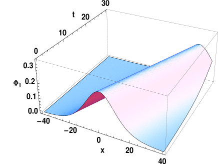
Figure 6: Hump soliton structure for $H<2$ is shown moving with supersonic speed in lab frame. The soliton hump corresponds to $T=10^{5}K$, $z=5$, $u_{0}=0.1$, $\varepsilon=0.1$ for which $H=0.64$, $n_{0}=3.5\times 10^{29}m^{-3}$, $\omega_{pe}=3.3\times 10^{16}s^{-1}$, respectively.

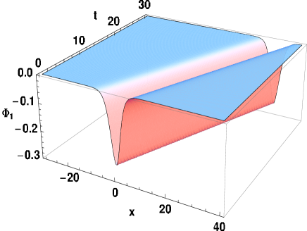
Figure 7: Dip soliton structure for $H>2$ is shown moving with subsonic speed in lab frame. The soliton dip is obtained at $T=10^{3}K$, $z=5$, $u_{0}=-0.1$, for which $H=2.03$, $n_{0}=3.5\times 10^{26}m^{-3}$, $\omega_{pe}=1.1\times 10^{15}s^{-1}$, respectively.

On the other hand, it is interesting to examine the conditions for weak coupling as deduced in the present theory. Combining the weak coupling condition yielding the minimal temperature in Eq. (17) with Eq. (49) gives an upper bound on the quantum diffraction parameter, or

$$H^{2}<H_{M}^{2}\equiv-\left(\frac{3}{\pi}\right)^{1/3}\frac{\mathrm{Li}_{-1/2}(-e^{\beta\mu_{0}})\mathrm{Li}_{5/2}(-e^{\beta\mu_{0}})}{[\mathrm{Li}_{3/2}^{2}(-e^{\beta\mu_{0}})]^{2/3}}\,,$$ (51)

which is shown in Fig. (8). It follows that large $H>2$ values fall within the strongly coupled regime where coupling parameter $g$ for degenerate electrons may become near or greater than one.

Figure 8: Maximal quantum parameter $H_{M}$ satisfying the weak coupling assumption, according to Eq. (51), where $z=e^{\beta\mu_{0}}$.

Nevertheless, considering ion-acoustic waves at least, a strong coupling between electrons will be not the main aspect of the dynamics. Although the complete analysis of the strongly coupled plasma regime is beyond the scope of this work, some conclusions can be found from the simplest way to introduce non-ideality for electrons, namely the addition of a dissipation term $-\omega_{coll}u_{e}$ in the right-hand side of Eq. (3), where $u_{e}$ is the electron fluid velocity and $\omega_{coll}$ is the electron-electron collision frequency. Using the continuity equation for electrons it is possible to estimate $\omega n_{e1}\approx k\,n_{0}u_{e1}$, where $n_{e1}$ and $u_{e1}$ are the first-order perturbations of the electron fluid density and velocity. Finally with $\omega\approx c_{s}k$ one finds that the dissipation term is negligible with respect to the pressure term provided $\omega\gg(m_{e}/m_{i})\omega_{coll}$, which is always satisfied within the inertialess electrons assumption. We note that according to the Landau expression r30 one has in the non-degenerate case

$$\frac{\omega_{coll}}{\omega_{pe}}\approx\frac{\ln\Lambda}{\Lambda}\,,$$ (52)

where $\Lambda\sim 1/g^{3/2}$ is the plasma parameter. In the fully degenerate case the right-hand side of Eq. (52) needs to be multiplied by the Pauli blocking factor $\kappa_{B}T/\varepsilon_{F}$. The conclusion is that except for very high $g\gg 1$ the electron-electron coupling can be neglected as long as the inertialess assumption is valid.

VI Conclusion

The linear and nonlinear ion-acoustic waves in a non-relativistic quantum plasma with arbitrary degeneracy of electrons have been investigated. Besides degeneracy, the quantum diffraction effect of electrons was also included, in terms of the Bohm potential. The linear dispersion relation for quantum ion-acoustic waves was found in terms of a generalized ion-acoustic speed, valid for both the dilute and dense cases. The numerical factor $\alpha$ in front of the quantum force in the macroscopic model was fixed in order to comply with the kinetic theory results. The corresponding KdV equation was obtained using the reductive perturbation method. The possible classes of propagating solitons, namely bright for $H<2$ moving with supersonic speed and dark for $H>2$ case moving with subsonic speed were discussed, where $H$ is a measure of the strength of quantum diffraction effects arising from the Bohm potential. To conclude, the derivation covers both the basic quantum effects in plasmas (arising resp. from quantum statistics and wave-like behavior of the charge carriers), in both the dilute and dense regimes. For instance, from Eq. (48) the scaled amplitude of the soliton becomes smaller for larger degeneracy, with $D=3u_{0}$ for $\alpha=1$ (non-degenerate case) and $D=9u_{0}/4$ for $\alpha=1/3$ (fully degenerate) case. The results are useful for the understanding of ion-acoustic wave propagation in an unmagnetized quantum plasma with arbitrary degeneracy of electrons.

- (1) S. H. Glenzer, O. L. Landen, P. Neumayer and R. W. Lee, Phys. Rev. Lett. 98, 065002 (2007).
- (2) A. K. Harding and D. Lai, Rep. Prog. Phys. 69, 2631 (2006).
- (3) A. Jüngel, Transport Equations for Semiconductors (Springer, Berlin, 2009).
- (4) F. Haas, Quantum Plasmas: an Hydrodynamic Approach (Springer, New York, 2011).
- (5) D. Melrose, Quantum Plasmadynamics - Unmagnetized Plasmas (Springer-Verlag, New York, 2008).
- (6) F. Haas, L. G. Garcia, J. Goedert and G. Manfredi, Phys. Plasmas 10, 3858 (2003).
- (7) G. Manfredi and F. Haas, Phys. Rev. B 64, 075316 (2001).
- (8) P. K. Shukla and S. Ali, Phys. Plasmas 12, 114502 (2005).
- (9) R. Sabry, W. M. Moslem and P. K. Shukla, Phys. Lett. A 372, 5691 (2008).
- (10) U. M. Abdelsalam, W. M. Moslem and P. K. Shukla, Phys. Plasmas 15, 052303 (2008).
- (11) A. E. Dubinov and A. A. Dubinova, Plasma Phys. Rep. 33, 859 (2007).
- (12) S. Mahmood and F. Haas, Phys. Plasmas 21, 102308 (2014).
- (13) A. E. Dubinov and A. A. Dubinova, Plasma Phys. Rep. 34, 403 (2008).
- (14) G. Manfredi and J. Hurst, Plasma Phys. Control. Fusion 57, 054004 (2015).
- (15) J. E. Cross, B. Reville and G. Gregori, Astrophys. J. 795, 59 (2014).
- (16) N. Maafa, Phys. Scripta 48, 351 (1993).
- (17) B. Eliasson and P.K. Shukla, J. Plasma Phys. 76, 7 (2010).
- (18) A. Mushtaq and D. B. Melrose, Phys. Plasmas 16, 102110 (2009).
- (19) D. B. Melrose and A. Mushtaq, Phys, Rev. E 82, 056402 (2010).
- (20) B. Eliasson and P. K. Shukla, Phys. Scripta 78, 025503 (2008).
- (21) A. E. Dubinov, A. A. Dubinova and M. A. Sazokin, J. Commun. Tech. Elec. 55, 907 (2010).
- (22) J. R. Barker and D. K. Ferry, Semicond. Sci. Technol. 13, A135 (1998).
- (23) C. L. Gardner, SIAM J. Appl. Math. 54, 409 (1994).
- (24) H. L. Rubin, T. R. Govindan, J. P. Kreskovski and M. A. Stroscio, Solid St. Electron. 36, 1697 (1993).
- (25) R. K. Pathria and P. D. Beale, Statistical Mechanics - 3rd ed. (Elsevier, New York, 2011).
- (26) L. Lewin, Polylogarithms and Associated Functions (North Holland, New York, 1981).
- (27) A. I. Akhiezer, I. A. Akhiezer, R. V. Polovin, A. G. Sitenko and K. N. Stepanov, Plasma Electrodynamics - vol. I (Pergamon, Oxford, 1975).
- (28) J. Zamanian, M. Marklund and G. Brodin, New J. Phys 12, 043019 (2010).
- (29) P. K. Shukla and B. Eliasson, Rev. Mod. Phys. 83, 885(2011).
- (30) A. P. Misra and P. K. Shukla, Phys. Rev. E 85, 026409 (2012).
- (31) D. Michta, F. Graziani and M. Bonitz, Contrib. Plasma Phys. 55, 437 (2015).
- (32) M. Akbari-Moghanjoughi, Phys. Plasmas 22, 022103 (2015).
- (33) D. Bohm and D. Pines, Phys. Rev. 92, 609 (1953).
- (34) R. C. Davidson, Methods in Nonlinear Plasma Theory (Academic Press, New York, 1972).
- (35) T. Kawahara, Phys. Soc. Japan 33, 260 (1972).
- (36) V. Yu. Belashov and S. V. Vladimirov, Solitary Waves in Dispersive Complex Media (Springer-Verlag, Berlin-Heidelberg, 2005).
- (37) E. M. Lifshitz and L. P. Pitaevskii, Physical Kinetics (Pergamon, Oxford, 1981).