A fixed-parameter algorithm for a routing open shop problem: unit processing times, few machines and locations

Abstract

The open shop problem is to find a minimum makespan schedule to process each job $J_{i}$ on each machine $M_{q}$ for $p_{iq}$ time such that, at any time, each machine processes at most one job and each job is processed by at most one machine. We study a problem variant in which the jobs are located in the vertices of an edge-weighted graph. The weights determine the time needed for the machines to travel between jobs in different vertices. We show that the problem with $m$ machines and $n$ unit-time jobs in $g$ vertices is solvable in $2^{\smash{O(gm^{2}\log gm)}}+O(mn\log n)$ time.

1 Introduction

Gonzalez and Sahni (1976) introduced the open shop problem: given a set $\mathcal{J}:=\{J_{1},\dots,J_{n}\}$ of jobs, a set $\mathcal{M}:=\{M_{1},\dots,M_{m}\}$ of machines, and the processing time $p_{iq}$ that job $J_{i}$ needs on machine $M_{q}$, the goal is to process each job on each machine in a minimum total amount of time such that each machine processes at most one job at a time and each job is processed by at most one machine at a time.

Averbakh et al (2006) introduced a problem variant where the jobs are located in the vertices of an edge-weighted graph. The edge weights determine the time needed for the machines to travel between jobs in different vertices. In their setting, all machines have the same travel speed and the travel times are symmetric. Initially, the machines are located in a vertex called the depot. The goal is to minimize the time needed for processing each job by each machine and returning all machines to the depot. This problem variant models, for example, scenarios where machines or specialists have to perform maintenance work on objects in several places. The travel times have also been interpreted as sequence-dependent machine-independent batch setup times (Allahverdi et al, 2008; Zhu and Wilhelm, 2006).

In order to formally define the problem, we first give a formal model for a transportation network and machine routes. Throughout this work, we use $\mathbb{N}:=\{0,1,\dots\}$.

Definition 1 (network, depot, routes)

A network $G=(V,E,c,v^{*})$ consists of a set $V$ of vertices and a set $E\subseteq\{\{u,v\}\mid u\neq v,u\in V,v\in V\}$ of edges such that $(V,E)$ is a connected simple graph, travel times $c\colon E\to\mathbb{N}\setminus\{0\}$, and a vertex $v^{*}\in V$ called the depot. We denote the number of vertices in a network by $g$.

A route with $s$ stays is a sequence $R:=(R_{k})_{k=1}^{s}$ of stays $R_{k}=(a_{k},v_{k},b_{k})\in\mathbb{N}\times V\times\mathbb{N}$ from time $a_{k}$ to time $b_{k}$ in vertex $v_{k}$ for $k\in\{1,\dots,s\}$ such that $v_{1}=v_{s}=v^{*}$, $a_{1}=0$,

$$a_{k} \leq b_{k} \text{for all }k\in\{1,\dots,s\},$$

$$\{v_{k},v_{k+1}\} \in E \text{for all }k\in\{1,\dots,s-1\}\text{, and}$$

$$a_{k+1} =b_{k}+c(v_{k},v_{k+1}) \text{for all }k\in\{1,\dots,s-1\}.$$

The length of $R$ is the end $b_{s}$ of the last stay.

Note that a route is actually fully determined by the $v_{k}$ and $b_{k}$ for each $k\in\{1,\dots,s\}$, yet it will be convenient to refer to both arrival time $a_{k}$ and departure time $b_{k}$ directly. We now define the routing open shop variant (ROS) introduced by Averbakh et al (2006).

Definition 2 (ROS)

An instance $I=(G,\mathcal{J},\mathcal{M},\allowbreak\text{loc},P)$ of the ROS problem consists of a network $G=(V,E,c,v^{*})$, a set $\mathcal{J}=\{J_{1},\dots,J_{n}\}$ of jobs, a set $\mathcal{M}=\{M_{1},\dots,M_{m}\}$ of machines, job locations $\text{loc}\colon\mathcal{J}\to V$, and an $(n\times m)$-matrix $P=(p_{iq})$ determining the processing time $p_{iq}\in\mathbb{N}$ of each job $J_{i}$ on each machine $M_{q}$.

A schedule $S\colon\mathcal{J}{}\times\mathcal{M}{}\to\mathbb{N}$ is a function determining the start time $S(J_{i},M_{q})$ of each job $J_{i}$ on each machine $M_{q}$. A job $J_{i}$ is processed by a machine $M_{q}$ in the half-open time interval $[S(J_{i},M_{q}),S(J_{i},M_{q})+p_{iq})$. A schedule is feasible if and only if

1. no machine $M_{q}$ processes two jobs $J_{i}\neq J_{j}$ at the same time, that is, $S(J_{i},M_{q})+p_{iq}\leq S(J_{j},M_{q})$ or $S(J_{j},M_{q})+p_{jq}\leq S(J_{i},M_{q})$ for all jobs $J_{i}\neq J_{j}$ and machines $M_{q}$,

2. no job $J_{i}$ is processed by two machines $M_{q}\neq M_{r}$ at the same time, that is, $S(J_{i},M_{q})+p_{iq}\leq S(J_{i},M_{r})$ or $S(J_{i},M_{r})+p_{ir}\leq S(J_{i},M_{q})$ for all jobs $J_{i}$ and machines $M_{q}\neq M_{r}$, and

3. there are routes $(R^{q})_{M_{q}\in\mathcal{M}}$ compatible with $S$, that is, for each job $J_{i}$ and each machine $M_{q}$ with route $R^{q}=(R_{k}^{q})_{k=1}^{s_{q}}$, there is a $k\in\{1,\dots,s\}$ such that $R_{k}^{q}=(a_{k}^{q},\text{loc}(J_{i}),b_{k}^{q})$ with $a_{k}^{q}\leq S(J_{i},M_{q})$ and $S(J_{i},M_{q})+p_{iq}\leq b_{k}^{q}$.

The makespan of a feasible schedule $S$ is the minimum value $L$ such that there are routes $(R_{M_{q}})_{M_{q}\in\mathcal{M}}$ compatible with $S$ and each having length at most $L$. An optimal solution to ROS is a feasible schedule with minimum makespan.

Note that a schedule for ROS only determines the start time of each job on each machine, not the times and destinations of machine movements. Yet the start times of each job on each machine fully determine the order in which each machine processes its jobs. Thus, one can easily construct compatible routes if they exist: each machine simply takes the shortest path from one job to the next if they are located in distinct vertices.

Preemption and unit processing times

The open shop problem is NP-hard even in the special cases of $m=3$ machines (Gonzalez and Sahni, 1976) or if all processing times are one or two (Kononov et al, 2011). Naturally, these results transfer to ROS with with $g=1$ vertex. ROS remains (weakly) NP-hard even for $g=m=2$ (Averbakh et al, 2006) and there are approximation algorithms both for this special and the general case of ROS (Averbakh et al, 2005; Yu et al, 2011; Chernykh et al, 2013; Kononov, 2015). However, the open shop problem is solvable in polynomial time if

1. job preemption is allowed, or

2. all jobs $J_{i}$ have unit processing time $p_{iq}=1$ on all machines $M_{q}$.

It is natural to ask how these results transfer to ROS. Regarding (1), Pyatkin and Chernykh (2012) have shown that ROS with allowed preemption is solvable in polynomial time if $g=m=2$, yet NP-hard for $g=2$ and an unbounded number $m$ of machines. Regarding (2), our work studies the following special case of ROS with unit execution times (ROS-UET):

Problem 1

By ROS-UET, we denote ROS restricted to instances where each job $J_{i}$ has unit processing time $p_{iq}=1$ on each machine $M_{q}$.

ROS-UET models scenarios where machines or specialists process batches of roughly equal-length jobs in several locations and movement between the locations takes significantly longer than processing each individual job in a batch. ROS-UET is NP-hard even for $m=1$ machine since it generalizes the metric travelling salesman problem. It is not obvious whether it is solvable in polynomial time even when both $g$ and $m$ are fixed. We show that, in this case, ROS-UET is solvable even in $O(n\log n)$ time, that is, ROS-UET is fixed-parameter tractable parameterized by $g+m$.

Fixed-parameter algorithms

Fixed-parameter algorithms are an approach towards efficiently and optimally solving NP-hard problems: the main idea is to accept the exponential running time for finding optimal solutions, yet to confine it to some small problem parameter $k$. A problem with parameter $k$ is called fixed-parameter tractable (FPT) if there is an algorithm that solves any instance $I$ in $f(k)\cdot|I|^{O(1)}$ time, where $f$ is an arbitrary computable function. The corresponding algorithm is called fixed-parameter algorithm. For more detail, we refer the reader to the recent text book by Cygan et al (2015).

Note that a fixed-parameter algorithm running in $O(2^{k}\cdot|I|)$ time runs in polynomial time for $k\in O(\log|I|)$, whereas an algorithm with running time $O(|I|^{k})$ runs in polynomial time only if $k$ is constant. The latter algorithm is not a fixed-parameter algorithm.

Recently, the field of fixed-parameter algorithmics has shown increased interest in scheduling and routing (Chen et al, 2017; van Bevern et al, 2016a, 2015a, 2015b, b; Bodlaender and Fellows, 1995; Fellows and McCartin, 2003; Halldórsson and Karlsson, 2006; Hermelin et al, 2015; Mnich and Wiese, 2015; van Bevern et al, 2017, 2014; Dorn et al, 2013; Gutin et al, 2017b, 2016, a, 2013; Jansen et al, 2017; Klein and Marx, 2014; Sorge et al, 2011, 2012), whereas fixed-parameter algorithms for problems containing elements of both routing and scheduling seem rare (Böckenhauer et al, 2007).

Input encoding

Encoding a ROS instance requires $\Omega(n\cdot m+g)$ bits in order to encode the processing time of each of $n$ jobs on each of $m$ machines and the travel time along each of at least $g-1$ edges. We call this the standard encoding. In contrast, a ROS-UET instance can be encoded using $O(g^{2}\cdot\log c_{\max}+g\cdot\log n)$ bits by encoding only the number of jobs in each vertex, where $c_{\max}$ is the maximum travel time. We call this the compact encoding.

All running times in this article are stated for computing a minimum makespan schedule, whose encoding requires $\Omega(n\cdot m)$ bits for the start time of each job on each machine. Thus, outputting the schedule is impossible in time polynomial in the size of the compact encoding. We therefore assume to get the input instance in standard encoding, like for the general ROS problem.

However, we point out that the decision version of ROS-UET is fixed-parameter tractable parameterized by $g+m$ even when assuming the compact encoding: our algorithm can decide whether there exists a schedule of given makespan $L$ in $2^{\smash{O(gm^{2}\log gm)}}\cdot|I|$ time if $I$ is a ROS-UET instance given in compact encoding (when replacing line 7 of Theorem 4.2 by “return $L$”, it will simply output the minimum makespan instead of constructing the corresponding schedule).

Organization of this work

In Section 2, we apply some basic preprocessing that allows us to assume that travel times satisfy the triangle inequality. In Section 3, we prove upper and lower bounds on the minimum makespan of schedules and on the number and length of stays of routes compatible with some optimal schedule. In Section 4, we present our fixed-parameter algortihm.

2 Preprocessing for metric travel times

In this section, we transform ROS instances into equivalent instances with travel times satisfying the triangle inequality. This will allow us to assume that, in an optimal schedule, a machine only stays in a vertex if it processes at least one job there: otherwise, it could take a “shortcut”, bypassing the vertex.

Lemma 1

Let $I$ be a ROS instance and let $I^{\prime}$ be obtained from $I$ by replacing the network $G=(V,E,c,v^{*})$ in $I$ by the network $G^{\prime}=(V,E^{\prime},c^{\prime},v^{*})$ such that $(V,E^{\prime})$ is a complete graph and $c^{\prime}:\{v,w\}\mapsto\text{dist}_{c}(v,w)$, where $\text{dist}_{c}(v,w)$ is the length of a shortest path between $v$ and $w$ in $G$ with respect to $c$.

Then, any feasible schedule for $I$ is a feasible schedule for $I^{\prime}$ with the same makespan and vice versa.

Proof

Clearly, any feasible schedule $S$ of makespan $L$ for $I$ is a feasible schedule of makespan at most $L$ for $I^{\prime}$. We show that any feasible schedule $S^{\prime}$ of makespan $L$ for $I^{\prime}$ is a feasible schedule of makespan at most $L$ for $I$. This is because, for any route $R^{\prime}$ compatible with $S^{\prime}$ in $I^{\prime}$, we get a route $R$ of the same length compatible with $S^{\prime}$ in $I$: between each pair of consecutive stays $(a_{i},v_{i},b_{i})$ and $(a_{i+1},v_{i+1},b_{i+1})$ on $R^{\prime}$ and a path $P=(w_{1}=v_{i},w_{2},\dots,w_{\ell}=v_{i+1})$ of length $c^{\prime}(v_{i},v_{i+1})$ with respect to $c$ in $G$, add zero-length stays in the vertices $w_{2},w_{3},\dots,w_{\ell-1}$ of $P$. This yields a route $R$ for $I$ of the same length as $R^{\prime}$ since the end of the last stay has not changed. ∎

The travel times $c^{\prime}$ in the network $G^{\prime}$ created in Lemma 1 satisfy the triangle inequality. Thus, one can assume that, except for the depot, a machine never visits a vertex of $G^{\prime}$ that has no jobs. Since one can delete such vertices, in the following, we will make the following simplifying assumption without loss of generality.

Assumption 2.1

Let $I$ be a ROS instance on a network $G=(V,E,c,v^{*})$. Then,

1. the travel times $c$ satisfy the triangle inequality,

2. each vertex $v\in V\setminus\{v^{*}\}$ contains at least one job.

3 Upper and lower bounds on makespan, number and lengths of stays

In this section, we show lower and upper bounds on the makespan of optimal ROS-UET schedules, as well as on the number and the lengths of stays of routes compatible with optimal schedules. These will be exploited in our fixed-parameter algorithm.

By Theorem 2.1(i), the travel times in the network $G$ of a ROS-UET instance satisfy the triangle inequality. Thus, the minimum cost of a cycle visiting each vertex of $G$ at least once coincides with the minimum cost of a cycle doing so exactly once (Serdyukov, 1978), that is, with that of a minimum-cost Hamiltonian cycle.

A trivial lower bound on the makespan of optimal ROS-UET schedules is given by the fact that, in view of Theorem 2.1(ii), each machine has to visit all vertices at least once and has to process $n$ jobs. A trivial upper bound is given by the fact that the machines can process the jobs sequentially. We thus obtain the following:

Observation 3.1

Let $I$ be a ROS-UET instance on a network $G=(V,E,c,v^{*})$ with a minimum-cost Hamiltonian cycle $H$. Then, the makespan of an optimal schedule to $I$ lies in $\{c(H)+n,\dots,c(H)+n+m-1\}.$

Moreover, a schedule with makespan $c(H)+n+m-1$ for ROS-UET is computable in $O(n\cdot m)$ time if a Hamiltonian cycle $H$ for the network of the input instance is also given as input.

We can improve the upper bound on the makespan if $c(H)<min\{n,m\}$:

Proposition 1

A feasible schedule of length $2c(H)+\max\{n,m\}$ for ROS-UET is computable in $O(m^{2}+mn+g)$ time if a Hamiltonian cycle $H$ for the network of the input instance is also given as input.

Proof

Without loss of generality, assume that $n\geq m$. Otherwise, we can simply add $m-n$ additional jobs to the depot and finally remove them from the constructed schedule. We will construct a feasible schedule $S$ of length $2c(H)+n$.

Let $H=(v_{1},v_{2},\ldots,v_{g},v_{1})$, where $v_{1}=v^{*}$ is the depot. Without loss of generality, let the jobs $J_{1},\dots,J_{n}$ be ordered so that, for jobs $J_{i},J_{j}$ with $i\leq j$, one has $\text{loc}(J_{i})=v_{k}$ and $\text{loc}(J_{j})=v_{\ell}$ with $k\leq\ell$. That is, the first jobs are in $v_{1}$, then follow jobs in $v_{2}$, and so on. We will construct our schedule from the matrix $S^{\prime}=(s^{\prime}_{iq})_{1\leq i\leq n,1\leq q\leq m}$, where

$$s^{\prime}_{iq} :=(i-q)\bmod n=\begin{cases}n-q+i&\text{ if $i<q$,}\\ i-q&\text{ otherwise.}\end{cases}$$ (1)

Figuratively, each row of $S^{\prime}$ is a cyclic right-shift of the previous row. Call a cell $s^{\prime}_{iq}$ red if $i<q$ and green otherwise. Note that, if $s^{\prime}_{iq}$ and $s^{\prime}_{jr}$ are of the same color and $i<j$ or $r<q$, then $s^{\prime}_{iq}<s^{\prime}_{jr}$. Moreover, the number in a red cell is larger than the number in any green cell in the same row or column: if $s^{\prime}_{iq}$ is red and $s^{\prime}_{jq}$ is green, then from

$$n+i >j\text{\quad follows}$$

$$s^{\prime}_{iq}=n-q+i >j-q=s^{\prime}_{jq}$$

and if $s^{\prime}_{iq}$ is red and $s^{\prime}_{ir}$ is green, then from

$$n-q >-r\text{\quad follows}$$

$$s^{\prime}_{iq}=n-q+i >i-r=s^{\prime}_{ir}.$$

Let $c_{k}=\sum_{i=2}^{k}c(v_{i-1},v_{i})$ be the travel time from $v_{1}$ to $v_{k}$ along $H$. Clearly, the sequence $(c_{k})_{k=1}^{s}$ is non-decreasing and $c_{g}\leq c(H)$. Our schedule $S$ is now given by

$$S(J_{i},M_{q})=s_{iq}:=s^{\prime}_{iq}+\begin{cases}c_{k}&\text{ if $\text{loc}(J_{i})=v_{k}$ and $s_{iq}$ is green},\\ c(H)+c_{k}&\text{ if $\text{loc}(J_{i})=v_{k}$ and $s_{iq}$ is red}.\end{cases}$$

Let us prove that this schedule is feasible in terms of Definition 2. Indeed, by construction, for two elements $s_{iq}$ and $s_{jr}$ with $i=j$ or $q=r$ and $s^{\prime}_{iq}>s^{\prime}_{jr}$, one has $s_{iq}>s_{jr}$ since the value added to $s^{\prime}_{iq}$ is not smaller than the value added to $s^{\prime}_{jr}$ due to our sorting of jobs by non-decreasing vertex indices and because the value added to any red cell is larger than any value added to a green cell. Therefore, conditions (i) and (ii) are satisfied.

It remains to verify (iii), that is, that there are compatible routes $R^{q}=((a_{k}^{q},v_{k}^{q},b_{k}^{q}))_{k=1}^{s_{q}}$ for each machine $M_{q}$. We let machine $M_{q}$ follow $H$ twice. During the first stay $(a_{k}^{q},v_{k}^{q},b_{k}^{q})$ in a vertex $v_{k}^{q}$, machine $M_{q}$ processes all jobs $J_{i}$ such that $s_{iq}$ is green. During the second stay $(a_{g+k}^{q},v_{k}^{q},b_{g+k}^{q})$, it processes all jobs $J_{i}$ such that $s_{iq}$ is red. By the choice of $s_{iq}$ for red cells, the machines have enough time to go around $H$ a second time. The length of the schedule is $n+2c(H)$: each machine uses $2c(H)$ time for traveling, $n$ time for processing the $n$ jobs, and is never idle. ∎

The machines in the proof of Proposition 1 visit vertices twice. The following example shows a ROS-UET instance for which Proposition 1 computes an optimal schedule and where the machines in an optimal schedule have to visit vertices repeatedly.

Example 1

Consider a ROS-UET instance on a network $G=(V,E,c,v^{*})$ with two vertices $v^{*}=v_{1}$ and $v_{2}$ and one edge $e=\{v_{1},v_{2}\}$ with $c(e)=t$. Vertex $v^{*}$ contains one job $J_{1}$, vertex $v_{2}$ contains $n-1$ jobs $J_{2},\dots,J_{n}$. A machine visiting $v_{2}$ only once either has to process first $J_{1}$ and then $J_{2},\dots,J_{n}$, or first all of $J_{2},\dots,J_{n}$ and then $J_{1}$.

Assume that we have $m=m_{1}+m_{2}$ machines, where a set $\mathcal{M}_{1}$ of $m_{1}$ machines processes $J_{1}$ first and a set $\mathcal{M}_{2}$ of $m_{2}$ machines processes $J_{1}$ last. Then one of the machines in $\mathcal{M}_{1}$ has to wait for the $m_{1}-1$ other machines in order to start $J_{1}$. Similarly, after finishing all jobs $J_{2},\dots,J_{n}$, one of the machines in $\mathcal{M}_{2}$ has to wait for the $m_{2}-1$ other machines in order to start $J_{1}$. Thus, this schedule has makespan at least $2t+n+m/2-1$: there is a machine that spends $2t$ time for travelling, $n$ time for processing, and at least $\max\{m_{1}-1,m_{2}-1\}\geq m/2-1$ time for idling.

Proposition 1 gives a schedule with makespan $4t+\max\{n,m\}$, which is smaller than $2t+n+m/2-1$ if $n\geq m\geq 4t-4$. Thus, in this instance, at least one machine in an optimal schedule has to visit $v_{2}$ twice, which incurs a travel time of $4t$. Since this machine also has to process $n$ jobs, it follows that the bound $4t+\max\{n,m\}=4t+n$ given by Proposition 1 is optimal in this case.

The above example shows that, in an optimal solution to ROS-UET, it can be necessary that machines visit vertices several times. The following lemma gives and upper bound on the number and length of stays of a machine in an optimal schedule.

Lemma 2

Let $S$ be an optimal schedule for a ROS-UET instance on a network $G=(V,E,c,v^{*})$. Let $L$ be the makespan of $S$ and $(R^{q})_{M_{q}\in\mathcal{M}}$ be routes of length at most $L$ compatible to $S$. Then, for each machine $M_{q}$, the route $R^{q}=((a_{k}^{q},v_{k}^{q},b_{k}^{q}))_{k=1}^{s_{q}}$

1. has at most $s_{q}\leq{m+2g-3}$ stays, and

2. the total length of the stays in any vertex $v\in V$ with $n_{v}$ jobs is

   $$\smashoperator[]{\sum_{1\leq k\leq s_{q},v_{k}^{q}=v}^{}}(b_{k}^{q}-a_{k}^{q})\leq n_{v}+m-1.$$ (2)

Proof

Let $H$ be a minimum-cost Hamiltonian cycle in $G$. We show that, if one of (i) or (ii) is violated, then $S$ has makespan at least $c(H)+m+n$, contradicting Theorem 3.1.

(i) If $R^{q}$ had at least $2g+m-2$ stays, then, by Proposition 4 in our graph-theoretic Appendix A, machine $M_{q}$ would be traveling for at least $c(H)+m$ time. Since the machine $M_{q}$ is processing jobs for $n$ time units, the makespan of $S$ is at least $c(H)+m+n$, a contradiction.

(ii) Machine $M_{q}$ takes at least $c(H)+n$ time just for visiting all vertices and processing all jobs. If (2) does not hold, then machine $M_{q}$ is neither travelling nor processing for at least $m$ time units. Thus, the length of route $R^{q}$ and, therefore, the makespan of $S$, is at least $c(H)+n+m$, again a contradiction. ∎

4 Fixed-parameter algorithm

In this section, we present a fixed-parameter algorithm for ROS-UET. The following simple algorithm shows that our main challenge will be “bottleneck vertices” that contain less jobs than there are machines.

Proposition 2

ROS-UET is solvable in $O(2^{g}g^{2}+mn)$ time if each vertex contains at least $m$ jobs.

Proof

First, compute a minimum-cost Hamiltonian cycle $H=(v_{1},v_{2},\dots,v_{g},v_{g+1})$ in the input network $G=(V,E,c,v^{*})$ in $O(2^{g}\cdot g^{2})$ time using the algorithm of Bellman (1962), Held and Karp (1962), where $v_{1}=v_{g+1}=v^{*}$ is the depot.

Denote by $n_{k}$ the number of jobs in $v_{k}$. Each machine will follow the same route $R$ of $g+1$ stays $(a_{1},v_{1},b_{1}),\dots,\allowbreak(a_{g+1},v_{g+1},b_{g+1})$, where $a_{1}:=0$, $b_{g+1}:=a_{g+1}$,

$$b_{k} :=a_{k}+n_{k} a_{k+1} :=b_{k}+c(v_{k},v_{k+1}) \text{for $k\in\{1,\dots,g\}$}.$$ and

That is, all machines will stay in vertex $v_{k}$ for the same $n_{k}$ time units. Now consider the schedule $S$ that schedules each job $J_{i}$ in a vertex $v_{k}$ on each machine $M_{q}$ at time

$$S(J_{i},M_{q})=a_{k}+(i-q)\bmod n_{k}.$$

Since $n_{k}\geq m$, it is easy to verify that $S(J_{i},M_{q})\neq S(J_{j},M_{r})$ for $i=j$ and $q\neq r$ and for $q=r$ and $i\neq j$ if $J_{i}$ and $J_{j}$ are in the same vertex $v_{k}$ (we did this for (1) in the proof of Proposition 1). For a job $J_{i}$ in a vertex $v_{k}$ and a job $J_{j}$ in a vertex $v_{\ell}$ with $k<\ell$, $S(J_{i},M_{q})\neq S(J_{j},M_{q})$ easily follows from $S(J_{i},M_{q})<a_{k}+n_{k}\leq a_{\ell}\leq S(J_{j},M_{q})$.

It is obvious that $S$ is compatible to route $R$. The length of $R$ is $c(H)+n$, which is optimal by Theorem 3.1. ∎

For the general ROS-UET problem, we prove the following theorem, which is our main algorithmic result.

Theorem 4.1

ROS-UET is solvable in $2^{O(gm^{2}\log gm)}+O(mn\log n)\text{ time.}$

In view of Proposition 2 and Example 1, the main challenge for our algorithm are “bottleneck vertices” with few jobs, which may force machines to idle.

Definition 3 (critical vertices, $n_{v}$)

For a vertex $v$ in the network of a ROS-UET instance, let $n_{v}$ denote the number of jobs in $v$. A vertex $v$ is critical if $n_{v}<m$.

To handle critical vertices, we exploit that, by Lemma 2, the $m$ routes compatible to an optimal schedule together have at most ${m^{2}+(2g-3)m}$ stays and stay in critical vertices last at most $2m-1$ time. In time that depends only on $g$ and $m$, we can thus try all possibly optimal chronological sequences of stays of machines in vertices, lengths of stays in critical vertices, and time differences between stays in critical vertices if they intersect. Thus, we can essentially try all possibilities of fixing everything in the routes except for the exact arrival and departure times of stays. For each such possibility, we will try to compute the arrival and departure times using integer linear programming, a schedule in critical vertices using brute force, and a schedule in uncritical vertices using edge colorings of bipartite graphs.

In the following, we first formalize these partially fixed schedules and routes and then give a description of our algorithm in pseudo-code.

Definition 4 (critical schedule)

A critical schedule is a function $S\colon\mathcal{J}{}\times\mathcal{M}{}\to\mathbb{N}\cup\{\bot\}$ determining the start time $S(J_{i},M_{q})\neq\bot$ of each job $J_{i}$ in a critical vertex on each machine $M_{q}$ and having $S(J_{i},M_{q})=\bot$ for all jobs $J_{i}$ in non-critical vertices.

A critical schedule has to satisfy Definition 2(i)–(iii) for all jobs $J_{i}$ and machines $M_{q}$ with $S(J_{i},M_{q})\neq\bot$.

We now formally define pre-schedules, which fix routes up to the exact arrival and departure times of stays. The definition is illustrated in Figure 1:

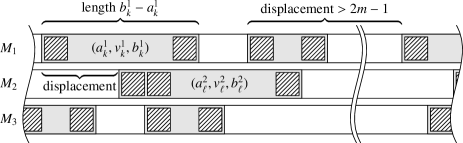
Figure 1: Shown is a part of a schedule for three machines $M_{1},M_{2}$, and $M_{3}$. The horizontal axis is time. Uniformly gray boxes are stays in critical vertices that comply with some pre-schedule (the pre-schedule is not shown). Hatched squares correspond to jobs being processed. Illustrated are the lengths of stays and displacements between stays in critical vertices that are consecutive in the pre-stay sequence (stays in non-critical vertices are not shown). Herein, this displacement is either smaller than $2m$, in which case the time difference between the stays is fixed for any complying set of routes, or at least $2m$, in which case the stays cannot intersect in time for any set of complying routes since stays in critical vertices have length at most $2m-1$ by Definition 5(iii).

Definition 5 (pre-schedule)

A pre-schedule is a triple $(T,A,D)$. Herein,

• is a pre-stay sequence $(T_{k})_{k=1}^{s}$ with $s\leq{m^{2}+(2g-3)m}$ and will fix a chronological order of all machine stays (by non-decreasing arrival times). The $k$-th pre-stay $T_{k}=(q_{k},w_{k})$ will require machine $M_{q_{k}}$ to stay in vertex $w_{k}$.

For the definition of the components $A$ and $D$ of a pre-schedule, let $\mathcal{K}\subseteq\{1,\dots,s\}$ be the indices $k$ of pre-stays $(q_{k},w_{k})$ such that $w_{k}$ is critical. Then,

• is called length assignment and will fix the length of the stay corresponding to the $k$-th pre-stay to be $A(k)$, and

• is called displacement and will fix the time difference between the stays corresponding to the $k$-th pre-stay and the previous pre-stay in a critical vertex to be $D(k)$ if $D(k)\leq 2m-1$ or to be at least $D(k)$ if $D(k)=2m$ (which means that it will prevent the two stays from intersecting).

We now formalize routes that comply with a pre-schedule. To this end, we denote by

• the number such that $(q_{k},w_{k})$ for some vertex $w_{k}$ is the $\sigma_{T,k}$-th pre-stay of machine $M_{q_{k}}$ in the pre-stay sequence $T$. We omit the subscript $T$ if the pre-stay sequence is clear from context.

Routes $(R^{q})_{M_{q}\in\mathcal{M}}$, where $R^{q}=((a_{k}^{q},v_{k}^{q},b_{k}^{q}))_{k=1}^{s_{q}}$, comply with the pre-stay sequence $T$ if and only if

1. $v^{q}_{\sigma_{k}}=w_{k}$ for all $k\in\{1,\dots,s\}$, that is, $M_{q}$ makes its $\sigma_{k}$-th stay in $w_{k}$, and

2. for pre-stays $({q_{k}},w_{k})$ and $({q_{\ell}},w_{\ell})$ with $k<\ell$, one has $a_{\sigma_{k}}^{q_{k}}\leq a_{\sigma_{\ell}}^{q_{\ell}}$, that is, the stays in all routes $(R^{q})_{M_{q}\in\mathcal{M}}$ are chronologically ordered according to $T$.

Routes $(R^{q})_{M_{q}\in\mathcal{M}}$ comply with a length assignment $A$ if,

1. each pre-stay $(q_{k},w_{k})$ in $T$ with $k\in\mathcal{K}$ has length $b_{\sigma_{k}}^{q_{k}}-a_{\sigma_{k}}^{q_{k}}=A(k)$.

Routes $(R^{q})_{M_{q}\in\mathcal{M}}$ comply with a displacement $D$ if

1. for two pre-stays $({q_{k}},v_{k})$ and $({q_{\ell}},v_{\ell})$ such that $k<\ell$, $\{k,\ell\}\subseteq\mathcal{K}$, and $i\notin\mathcal{K}$ for each $i\in\{k+1,\dots,\ell-1\}$, one has

   $$a_{\sigma_{\ell}}^{q_{\ell}} \geq a_{\sigma_{k}}^{q_{k}}+2m D(j)=2m$$ if  and

   $$a_{\sigma_{\ell}}^{q_{\ell}} =a_{\sigma_{k}}^{q_{k}}+D(\ell) D(j)<2m$$ if .

Routes comply with $(T,A,D)$ if they comply with each of $T$, $A$, and $D$.

Lemma 2 implies that there is a pre-schedule complying with some routes compatible to an optimal schedule. We thus enumerate all possible pre-schedules and, for each, try to find routes complying with the pre-schedule and compatible to an optimal schedule. This leads to the following algorithm.

Algorithm 4.2

Input:

A ROS-UET instance $I=(G,\mathcal{J},\mathcal{M},\text{loc},P)$ on a network $G=(V,E,c,v^{*})$.

Output:

A minimum-makespan schedule for $I$.

1. Preprocess $G$ to establish the triangle inequality. // Lemma 1

2. $H\leftarrow{}$minimum-cost Hamiltonian cycle $H$ in $G$.

3. for $L=c(H)+n$ to $c(H)+n+m-1$ do // Try to find schedule with makespan $L$ (Obs. 3.1)

4. foreach pre-schedule $(T,A,D)$ do // Lemma 3

5. if there are routes $(R^{q})_{M_{q}\in\mathcal{M}}$ that comply with $(T,A,D)$, // Lemma 4

   that have length at most $L$ each, and

   stay in each non-critical vertex $v\in V$ at least $n_{v}$ time, then

6. if there is a critical schedule $S^{\prime}$ compatible with $(R^{q})_{M_{q}\in\mathcal{M}}$, then // Lemma 5

7. complete $S^{\prime}$ into a feasible schedule $S$ compatible with $(R^{q})_{M_{q}\in\mathcal{M}}$. // Lemma 6

8. return $S^{\prime}$.

To prove the correctness and the running time of Theorem 4.2, we prove the lemmas named in its comments. We already proved Lemmas 1 and 3.1 and we continue proving lemmas in the order appearing in the algorithm. First, we bound the number of pre-schedules and thus the number of repetitions of the loop in line 4.

Lemma 3

In line 4 of Theorem 4.2, there are at most $2^{O(m^{2}\log gm+mg\log gm)}$ pre-schedules, which can be enumerated in $2^{O(m^{2}\log gm+mg\log gm)}$ time.

Proof

There are at most $(mg)^{m^{2}+(2g-3)m}$ pre-stay sequences: a pre-stay sequence consists of at most ${m^{2}+(2g-3)m}$ pre-stays, each of which is a pair of one of $m$ machines and one of $g$ vertices. For each pre-stay sequence, there are at most $(2m)^{m^{2}+(2g-3)m}$ length assignments and at most $(2m+1)^{m^{2}+(2g-3)m}$ displacements. Thus, the number of pre-schedules is at most $(4gm^{3}+2gm^{2})^{m^{2}+(2g-3)m}=2^{({m^{2}+(2g-3)m})\log(4gm^{3}+2gm^{2})}$. They can obviously be enumerated in the stated running time using a recursive algorithm. ∎

We realize the check in line 5 by testing the feasibility of an integer linear program whose number of variables, number of constraints, and absolute value of coefficients is bounded by $O({m^{2}+(2g-3)m})$. By Lenstra’s theorem, this works in $2^{O(m^{2}\log gm+mg\log gm)}$ time:

Proposition 3 (Lenstra (1983); see also Kannan (1987))

A feasible solution to an integer linear program of size $n$ with $p$ variables is computable using $p^{O(p)}\cdot n$ arithmetical operations, if such a feasible solution exists.

Lemma 4

The routes in line 5 of Theorem 4.2 are computable in $2^{O(m^{2}\log gm+mg\log gm)}$ time, if they exist.

Proof

Let $T:=(({q_{k}},w_{k}))_{i=1}^{s}$ be the pre-stay sequence in the pre-schedule $(T,A,D)$ enumerated in line 4. By $s_{q}$, denote the number of pre-stays of a machine $M_{q}$ in $T$. We compute the routes $(R^{q})_{M_{q}\in\mathcal{M}}$, where $R^{q}:=((a_{k}^{q},v_{k}^{q},b_{k}^{q}))_{k=1}^{s_{q}}$, as follows. For each pre-stay $({q_{k}},w_{k})$ on $T$, we let $v_{\sigma_{k}}^{q_{k}}:=w_{k}$. If $v_{1}^{q}\neq v^{*}$ or $v^{*}\neq w_{s_{q}}^{q}$ for some machine $M_{q}$, where $v^{*}$ is the depot, then there are no routes complying with $(T,A,D)$ and we return “no” accordingly.

Otherwise, by Definition 5, the $a_{k}^{q}$ and $b_{k}^{q}$ for all machines $M_{q}$ and $1\leq k\leq s_{q}$ together are at most $2m\cdot({m+2g-3})$ variables. They can be determined by a feasible solution to an integer linear program. This, together with Proposition 3 directly yields the running time stated in Lemma 4. The linear program consists of the following constraints. We want each route to have length at most $L$, that is,

$$b_{s_{q}}^{q} \leq L \text{for each $M_{q}\in\mathcal{M}$}.$$

The difference between departure and arrival times are the travel times, that is,

$$b_{k}^{q}+c(v_{k}^{q},v_{k+1}^{q}) =a_{k+1}^{q} M_{q}\in\mathcal{M} 1\leq k\leq s_{q}-1$$ for each and .

Stays should have non-negative length, that is,

$$a_{k}^{q} \leq b_{k}^{q} M_{q}\in\mathcal{M} 1\leq k\leq s_{q}$$ for each and .

Each machine should stay in $$v\in V n_{v}$$ for at least  time, that is

$$\sum_{\begin{subarray}{c}1\leq k\leq s_{q}\\ w_{k}^{q}=v\end{subarray}}(b_{k}^{q}-a_{k}^{q}) \geq n_{v} M_{q}\in\mathcal{M} v\in V$$ for each  and .

Stays must be ordered according to the pre-stay sequence $$T$$, that is

$$a_{\sigma_{k}}^{q_{k}} \leq a_{\sigma_{\ell}}^{q_{\ell}} ({q_{k}},v_{k}) ({q_{\ell}},v_{\ell}) k\leq\ell$$ for pre-stays and with .

Stays should adhere to the length assignment $$A$$, that is

$$b_{\sigma_{k}}^{q_{k}}-a_{\sigma_{k}}^{q_{k}} =A(k) ({q_{k}},v_{k}) v_{k}$$ for each pre-stay such that  is critical.

Finally, routes have to comply with the displacement $$D \mathcal{K} T ({q_{k}},w_{k}) ({q_{\ell}},w_{\ell}) k<\ell \{k,\ell\}\subseteq\mathcal{K} i\notin\mathcal{K} i\in\{k+1,\dots,\ell-1\}$$. To formulate the constraint, let be the indices of pre-stays of  in critical vertices. For any two pre-stays and with , , and for each , we want

$$a_{\sigma_{\ell}}^{q_{\ell}} \geq a_{\sigma_{k}}^{q_{k}}+D(\ell) D(\ell)=2m$$ if , and

$$a_{\sigma_{\ell}}^{q_{\ell}} =a_{\sigma_{k}}^{q_{k}}+D(\ell) \text{if $D(\ell)<2m$.}\hskip 142.26378pt\qed$$

Next, we show how to realize the check in 6 of Theorem 4.2.

Lemma 5

The critical schedule $S^{\prime}$ in line 6 is computable in $2^{O(gm^{2}\log m)}$ time, if such a schedule exists.

Proof

In total, there are at most $g\cdot m$ jobs in critical vertices. Thus, we determine the starting time $S(J_{i},M_{q})$ for at most $g\cdot m^{2}$ pairs $(J_{i},M_{q})\in\mathcal{J}\times\mathcal{M}$. By Lemma 2, each machine can process all of its jobs in a critical vertex staying there no longer than $2m-1$ units of time. Thus, for each of at most $g\cdot m^{2}$ pairs $(J_{i},M_{q})$, we enumerate all possibilities of choosing $S(J_{i},M_{q})$ among the smallest $2m-1$ time units where $M_{q}$ stays in vertex $\text{loc}(J_{i})$.

There are $(2m-1)^{g\cdot m^{2}}\in 2^{O(gm^{2}\log m)}$ possibilities to do so. The feasibility’s of each variant can be checked in $O(g\cdot m^{2})$ time and they can all be enumerated in $2^{O(gm^{2}\log m)}$ total time: since the routes $(R^{q})_{M_{q}\in\mathcal{M}}$ comply with $(T,A,D)$, they have at most ${m^{2}+(2g-3)m}$ stays in total, thus we can list the first $2m-1$ time units that a concrete machine stays in a concrete vertex in $(2m-1)+{m^{2}+(2g-3)m}$ time. ∎

In the following, we provide the last building block for proving the correctness and the running time of Theorem 4.2: Lemma 2 already shows that there is a pre-schedule that complies with some routes that are compatible with an optimal schedule. Thus, it is sufficient to try, for each pre-schedule $(T,A,D)$, to search for schedules compatible with routes complying with $(T,A,D)$. However, the algorithm only searches for schedules compatible to one collection of machine routes complying with $(T,A,D)$. The following lemma shows that this is sufficient.

Lemma 6

If a ROS-UET instance on a network $G=(V,E,c,v^{*})$ allows for a feasible schedule compatible to routes complying with a pre-schedule $(T,A,D)$, then

1. for any collection of routes $(R^{q})_{M_{q}\in\mathcal{M}}$ complying with $(T,A,D)$, there is a critical schedule compatible with $(R^{q})_{M_{q}\in\mathcal{M}}$, and

2. any such critical schedule can be extended into a feasible schedule compatible to $(R^{q})_{M_{q}\in\mathcal{M}}$ if each route $R^{q}$ stays in each vertex $v$ for at least $n_{v}$ time.

Moreover, line 7 can be carried out in $O(m^{2}+gm+mn\log n)$ time.

Proof

(i) Let $S^{*}$ be a feasible schedule compatible to some routes $(R^{q*})_{M_{q}\in\mathcal{M}}$ complying with $(T,A,D)$. Denote the pre-stay sequence $T=(({q_{k}},w_{k}))_{k=1}^{s}$. We show how to construct a critical schedule $S$ compatible with respect to the routes $(R_{M_{q}})_{M_{q}\in\mathcal{M}}$. Denote $\smash{R^{q*}=((a^{q*}_{k},v^{q*}_{k},b^{q*}_{k}))_{k=1}^{s_{q}^{*}}}$, and $R^{q}=((a_{k}^{q},v_{k}^{q},b_{k}^{q}))_{k=1}^{s_{q}}$ for each machine $M_{q}$. By Definition 5(i) and Definition 2(iii), for each job $J_{i}$ and machine $M_{q}$ there is an index $P(J_{i},M_{q}):=p$ of a pre-stay $({q_{p}},w_{p})=(q,\text{loc}(J_{i}))$ on $T$ such that

$$a^{q*}_{\sigma_{p}}\leq S^{*}(J_{i},M_{q})<b^{q*}_{\sigma_{p}}.$$ (3)

Since the routes $(R^{q*})_{M_{q}\in\mathcal{M}}$ and $(R^{q})_{M_{q}\in\mathcal{M}}$ comply with $T$, by Definition 5(i), one has $s_{q}=s^{*}_{q}$ and, moreover, $v_{k}^{q}=v_{k}^{q*}$ for each machine $M_{q}$ and $1\leq k\leq s_{q}$. For each job $J_{i}$ and machine $M_{q}$, we define

$$S(J_{i},M_{q}):=\begin{cases}\bot&\text{if $\text{loc}(J_{i})$\leavevmode\nobreak\ is not critical},\\ S^{*}(J_{i},M_{q})-a^{q*}_{\sigma_{p}}+a^{q}_{\sigma_{p}}&\text{otherwise,}\end{cases}$$

where $p=P(J_{i},M_{q})$.

We show that $S$ is a critical schedule compatible with the routes $(R^{q})_{M_{q}\in\mathcal{M}}$. For each job $J_{i}$ in a critical vertex and each machine $M_{q}$, we first show that machine $M_{q}$ stays in $\text{loc}(J_{i})$ when processing job $J_{i}$. More precisely, for $p=P(J_{i},M_{q})$, we show $a^{q}_{\sigma_{p}}\leq S(J_{i},M_{q})<b^{q}_{\sigma_{p}}$ as follows. By adding $-a^{q*}_{\sigma_{p}}+a^{q}_{\sigma_{p}}$ to both sides of

$$a^{q*}_{\sigma_{p}}\leq S^{*}(J_{i},M_{q}),$$

which holds since $p$ is chosen so as to satisfy (3), one gets

$$a^{q}_{\sigma_{p}}\leq S^{*}(J_{i},M_{q})-a^{q*}_{\sigma_{p}}+a^{q}_{\sigma_{p}}=S(J_{i},M_{q}).$$

Moreover, since both $R^{q*}$ and $R^{q}$ comply with the length assignment $A$, by Definition 5(iii), one has $b_{\sigma_{k}}^{q_{k}}-a_{\sigma_{k}}^{q_{k}}=A(k)=b^{q_{k}*}_{\sigma_{k}}-a^{q_{k}*}_{\sigma_{k}}$ for all pre-stays $({q_{k}},w_{k})$ such that $w_{k}$ is critical. Thus, by adding $-a^{q*}_{\sigma_{p}}+a^{q}_{\sigma_{p}}$ to both sides of

$$S^{*}(J_{i},M_{q})<b^{q*}_{\sigma_{p}},$$

which holds since $p$ is chosen so as to satisfy (3), one gets

$$S(J_{i},M_{q})=S^{*}(J_{i},M_{q})-a^{q*}_{\sigma_{p}}+a^{q}_{\sigma_{p}}<b^{q*}_{\sigma_{p}}-a^{q*}_{\sigma_{p}}+a^{q}_{\sigma_{p}}=b^{q}_{\sigma_{p}}.$$

It remains to show that $S^{*}$ processes no two jobs at the same time and that no two machines process one job at the same time. To this end, consider jobs $J_{i},J_{j}$ in critical vertices and machines $M_{q},M_{r}$. If either $i=j$ or $q=r$, then $S^{*}(J_{i},M_{q})\neq S^{*}(J_{j},M_{r})$. Thus, it is sufficient to show that $S^{*}(J_{i},M_{q})\neq S^{*}(J_{j},M_{r})$ implies $S(J_{i},M_{q})\neq S(J_{j},M_{r})$. To this end, let $p:=P(J_{i},M_{q})$ and $\pi:=P(J_{j},M_{r})$. Without loss of generality, assume that $p\leq\pi$. By Definition 5(ii), one has $a^{q}_{\sigma_{p}}\leq a^{r}_{\sigma_{\pi}}$.

If $b_{\sigma_{p}}^{q}\leq a^{r}_{\sigma_{\pi}}$, then $S(J_{i},M_{q})\neq S(J_{r},M_{r})$ follows from $S(J_{i},M_{q})<b^{q}_{\sigma_{p}}\leq a^{r}_{\sigma_{\pi}}\leq S(J_{j},M_{r}).$ Otherwise, since $b^{q}_{\sigma_{p}}-a^{q}_{\sigma_{p}}=A(p)\leq 2m-1$ by Definition 5(iii), one has $a^{r}_{\sigma_{\pi}}-a^{q}_{\sigma_{p}}\leq b^{q}_{\sigma_{p}}-a^{q}_{\sigma_{p}}\leq 2m-1$. Thus, for $\mathcal{K}(p,\pi]:=\{k\in\{p+1,\dots,\pi\}\mid({q_{k}},w_{k})$ is a pre-stay of $T$ in a critical vertex$\}$, one has, by Definition 5(ii) and (iv),

$$a^{r}_{\sigma_{\pi}}-a^{q}_{\sigma_{p}}=\smashoperator[]{\sum_{k\in\mathcal{K}(p,\pi]}^{}}D(k)=a^{r*}_{\sigma_{\pi}}-a_{\sigma_{p}}^{q*}$$ (4)

since both tours $(R^{q})_{M_{q}\in\mathcal{M}}$ and $(R^{q*})_{M_{q}\in\mathcal{M}}$ comply with the displacement $D$. By adding $a^{r}_{\sigma_{\pi}}-a^{q*}_{\sigma_{p}}$ to both sides of

$$S(J_{i},M_{q})+a^{q*}_{\sigma_{p}}-a^{q}_{\sigma_{p}} =S^{*}(J_{i},M_{q})\neq S^{*}(J_{j},M_{r})=S(J_{j},M_{r})+a^{r*}_{\sigma_{\pi}}-a^{r}_{\sigma_{\pi}},$$

which is true by the definition of $S$ from $S^{*}$, one obtains

$$S(J_{i},M_{q})+a^{r}_{\sigma_{\pi}}-a^{q}_{\sigma_{p}}\neq S(J_{r},M_{r})+a^{r*}_{\sigma_{\pi}}-a^{q*}_{\sigma_{p}},$$

and, therefore, $S(J_{i},M_{q})\neq S(J_{j},M_{r})$ from (4).

(ii) We complete any critical schedule $S^{\prime}$ compatible with the routes $(R^{q})_{M_{q}\in\mathcal{M}}$ into a feasible schedule compatible with $(R^{q})_{M_{q}\in\mathcal{M}}$ as follows.

For each machine $M_{q}$ and each non-critical vertex $v$, let $T_{qv}\subseteq\mathbb{N}$ be a set of $n_{v}$ arbitrary times where machine $M_{q}$ stays in $v$ according to route $R^{q}$ and let $T_{v}:=\bigcup_{M_{q}\in\mathcal{M}}T_{qv}$. For each vertex $v\in V$, create a bipartite graph $G_{v}=(\mathcal{M}\cup T_{v},E_{v})$, where $E_{v}$ contains an edge $\{M_{q},t\}$ between a machine $M_{q}$ and a time $t\in T_{qv}$ if and only if $M_{q}$ is in $v$ at time $t$. Each vertex of $G_{v}$ has degree $n_{v}$ or $m$, where $m\leq n_{v}$ since $v$ is non-critical. Thus, $G_{v}$ allows for a proper edge coloring $c_{v}\colon E_{qv}\to\{1,\dots,n_{v}\}$: if one of $q=r$ or $t=t^{\prime}$, then $c_{v}(\{M_{q},t\}\neq c_{v}(\{M_{r},t^{\prime}\})$. This coloring will tell us which job machine $M_{q}$ will process at time $t$. Let the jobs in each vertex $v$ be $\{J_{1}^{v},\dots,J_{n_{v}}^{v}\}$. Then, for any machine $M_{q}$ and job $J_{j}^{v}$ in a non-critical vertex $v$, there is a unique $t_{qj}$ such that $c_{v}(\{M_{q},t_{qj}\})=j$. We thus define our schedule $S$ as

$$S(J_{i},M_{q}):=\begin{cases}S^{\prime}(J_{i},M_{q})&\text{ if $J_{i}$ is in a critical vertex}\\ t_{qj}&\text{ if $J_{i}=J_{j}^{v}$ for some non-critical vertex\leavevmode\nobreak\ $v$}.\end{cases}$$

By construction from schedule $S^{\prime}$ for critical vertices, which is compatible to the routes $(R^{q})_{M_{q}\in\mathcal{M}}$, and from the edge-coloring $c_{v}$ for non-critical vertices $v$, schedule $S$ is compatible to $(R^{q})_{M_{q}\in\mathcal{M}}$. Moreover, from this, $S(J_{i},M_{q})\neq S(J_{j},M_{q})$ follows if $J_{i}\neq J_{j}$ are in the same vertex. If $J_{i}\neq J_{j}$ are in different vertices, then this follows from the compatibility of $S$ with the routes $(R^{q})_{M_{q}\in\mathcal{M}}$: machine $M_{q}$ cannot stay in two vertices at the same time. Finally, $S(J_{i},M_{q})\neq S(J_{i},M_{r})$ for $M_{q}\neq M_{r}$ follows from $S^{\prime}(J_{i},M_{q})\neq S^{\prime}(J_{i},M_{r})$ if $J_{i}$ is in a critical vertex. If $J_{i}$ is a job in a non-critical vertex, say $J_{j}^{v}$, then $S(J_{i},M_{q})=S(J_{j},M_{r})$ implies $t_{qj}=t_{rj}$ and, in turn, $c_{v}(\{M_{r},t_{qj}\})=j=c_{v}(\{M_{r},t_{rj}\})$, contradicting the fact that $c_{v}$ is a proper edge coloring.

We analyze the running time for this completion step. Since the routes $(R^{q})_{M_{q}\in\mathcal{M}}$ have at most ${m^{2}+(2g-3)m}$ stays, one can compute the sets $T_{vq}$ for all vertices $v$ and machines $M_{q}$ in $O({m^{2}+(2g-3)m}+n)$ time. For each vertex $v$, the bipartite graph $G_{v}$ can be generated in $O(mn_{v})$ time and an edge-coloring into $n_{v}$ colors can be computed in $O(mn_{v}\log n_{v})$ time (Cole et al, 2001). Thus, in total, we can compute schedule $S$ in

$$O({m^{2}+(2g-3)m}+n)+\sum_{v\in V}O(mn_{v}\log n_{v})=O(m^{2}+gm+mn\log n)\text{\quad time.}\qquad\qed$$

We can now prove the correctness and running time of Theorem 4.2.

Proof (of Theorem 4.1)

Let $L^{*}$ be the makespan of an optimal schedule $S^{*}$ for the ROS-UET instance input to Theorem 4.2. We only have to show that (and in which time) Theorem 4.2 outputs a feasible schedule $S$ with makespan at most $L^{*}$. To this end, let $(R^{q*})_{M_{q}\in\mathcal{M}}$ be routes compatible to $S^{*}$, each of length at most $L^{*}$. Line 1 of Theorem 4.2 can be carried out in $O(g^{3})$ time using the Floyd-Warshall algorithm, line 2 in $O(2^{g}g^{2})$ time using the algorithm of Bellman (1962), Held and Karp (1962). By Theorem 3.1, $L=L^{*}$ in at least one iteration of the loop in line 3. We now consider this iteration. By Lemma 3, in line 4, we enumerate $2^{O(m^{2}\log gm+mg\log gm)}$ pre-schedules. By Lemma 2, among them there is a pre-schedule $(T^{*},A^{*},D^{*})$ that complies with $(R^{q*})_{M_{q}\in\mathcal{M}}$. Since $S^{*}$ processes all jobs, the routes $(R^{q*})_{M_{q}\in\mathcal{M}}$ stay in each vertex $v$ at least $n_{v}$ time. Thus, the test in line 5 succeeds for $(T^{*},A^{*},D^{*})$ and $L=L^{*}$ and, by Lemma 4, can be carried out in $2^{O(m^{2}\log gm+mg\log gm)}$ time. By Lemma 5 the test in line 6 can be carried out in $2^{O(gm^{2}\log m)}$ time and, by Lemma 6(i), it succeeds. We get the the feasible schedule $S$ in line 7 in $O(m^{2}+gm+mn\log n)$ time by Lemma 6(ii). Its makespan is at most $L=L^{*}$. The overall running time of the algorithm is $O(g^{3}+2^{g}g^{2})+m\cdot 2^{O(m^{2}\log gm+mg\log gm)}\cdot(2^{O(m^{2}\log gm+mg\log gm)}+2^{O(gm^{2}\log m)})+O(m^{2}+gm+mn\log n)$.∎

5 Open questions

We have shown that ROS-UET is fixed-parameter tractable with respect to the parameter $m+g$ and, in the absence of critical vertices, also with respect to the parameter $g$. However, the question whether ROS-UET with critical vertices and an unbounded number of machines is polynomial-time solvable is open even for two vertices.

Appendix A On the minimum weight of long closed walks containing all vertices

In the following, we prove Proposition 4, which we used to prove Lemma 2. For its formal statement and proof, we have to formally distinguish two different kinds of paths and cycles:

Definition 6 (closed walks, cycles)

Let $G=(V,E)$ be a multigraph with edge weights $c\colon E\to\mathbb{N}$. A walk of length $\ell$ in $G$ is an alternating sequence $(v_{1},e_{1},v_{2},e_{2},\dots,v_{\ell},e_{\ell},v_{\ell+1})$ of vertices and edges such that $v_{i}$ and $v_{i+1}$ are the end points of $e_{i}$ for each $i\in\{1,\dots,\ell\}$. Its weight is $\sum_{i=1}^{\ell}c(e_{i})$, its internal vertices are $v_{2},\dots,v_{\ell}$, and it is closed if $v_{1}=v_{\ell+1}$.

A graph is Eulerian if it contains an Euler tour—a closed walk that contains each edge of $G$ exactly once. It is known that a connected undirected multigraph is Eulerian if and only if each vertex has even degree. A (simple) path is a walk that contains each edge and internal vertex at most once. A cycle is a closed path.

Proposition 4

Let $G$ be a connected $n$-vertex graph with positive integer edge weights and let $T$ be a closed walk of length $2n-2+k$ containing all vertices of $G$. Then, the weight of $T$ is at least $W+k$, where $W$ is the minimum weight of any closed walk containing all vertices of $G$.

To prove Proposition 4, we exploit the following theorem.

Theorem A.1 (Mader (1974, Satz 1))

Every simple graph with minimum degree $k\geq 2$ contains a cycle $C$ such that there are $k$ mutually internally vertex-disjoint paths between any pair of vertices of $C$.

Corollary 1

Let $G$ be a connected $n$-vertex multigraph without loops such that the deletion of the edges of any cycle disconnects $G$. Then $G$ has at most $2n-2$ edges.

Proof

We prove the statement by induction on $n$. The statement is trivial for $n=1$, since such a graph has no edges. Now, let $n>1$. If $G=(V,E)$ contains a cutset $E^{\prime}\subseteq E$ of cardinality at most 2 (that it, its deletion disconnects the graph), then $G\setminus E^{\prime}=(V,E\setminus E^{\prime})$ consists of two connected components $G_{1}$ and $G_{2}$. By induction, we have $|E(G)|=|E(G_{1})|+|E(G_{2})|+|E^{\prime}|\leq 2|V(G_{1})|-2+2|V(G_{2})|-2+2=2n-2$. It remains to prove that $G=(V,E)$ indeed contains a cutset $E^{\prime}\subseteq E$ of cardinality at most 2.

If $G$ contains a vertex $v$ of degree at most 2, then its incident edges form the sought cutset of cardinality 2. If $G$ contains at least two distinct edges $e_{1}$ and $e_{2}$ between the same pair $u$ and $v$ of vertices, then $(u,e_{1},v,e_{2},u)$ is a cycle and, thus, $E^{\prime}=\{e_{1},e_{2}\}$ is the sought cutset of cardinality 2.

If none of the above apply, then $G$ is a simple graph with minimum degree three. Thus, by Theorem A.1, $G$ contains a cycle $C$ whose edges can be deleted without disconnecting the graph: deleting the edges of $C$ removes at most two out of three pairwise internally vertex-disjoint paths between any pair of vertices of $C$. This contradicts our assumption that deleting the edges of any cycle disconnects $G$. ∎

We can now prove Proposition 4.

Proof (of Proposition 4)

Consider the following multigraph $H$: the vertices of $H$ are the vertices of $G$ and the number of edges in $H$ between each pair $u$ and $v$ of vertices is equal to the number of times the closed walk $T$ contains the edge $\{u,v\}$ of $G$. The multigraph $H$ is connected, Eulerian, has $n$ vertices and $2n-2+k$ edges. If $k>0$, then, by Corollary 1, there is a cycle $C$ in $H$ whose removal results in a connected multigraph $H^{\prime}$. Multigraph $H^{\prime}$ is still Eulerian. Thus, we can iterate the process until we get an Eulerian submultigraph $H^{*}$ of $H$ with at most $2n-2$ edges. The Euler tour $T^{*}$ of $H^{*}$ is a closed walk for $G$ containing all its vertices and thus has weight at least $W$. Since the total weight of the deleted cycles is at least $k$, the weight of $T$ is at least $W+k$. ∎

Finally, note that the bound given by Proposition 4 is tight for each $n$ and even $k$: consider a unit-weight path graph $G$ on $n$ vertices $v_{1},\dots,v_{n}$. The minimum weight of any closed walk containing all vertices is $W:=2n-2$. The closed walk visiting the vertices $v_{1},v_{2},\dots,v_{n-1},v_{n},v_{n-1},\dots,v_{2},v_{1},v_{2},\dots,v_{k^{\prime}-1},v_{k^{\prime}},v_{k^{\prime}-1},\dots,\allowbreak v_{2},v_{1}$ with $k^{\prime}:=(k+2)/2$ in this order has length $2n-2+2k^{\prime}-2=2n-2+k$ and its weight is $W+2k^{\prime}-2=W+k$.