Numerical solution of an ill-posed Cauchy problem for a quasilinear parabolic equation using a Carleman weight function

Abstract

This is the first publication in which an ill-posed Cauchy problem for a quasilinear PDE is solved numerically by a rigorous method. More precisely, we solve the side Cauchy problem for a 1-d quasilinear parabolc equation. The key idea is to minimize a strictly convex cost functional with the Carleman Weight Function in it. Previous publications about numerical solutions of ill-posed Cauchy problems were considering only linear equations.

Key Words: Ill-posed Cauchy problem, quasilinear parabolic PDE, numerical solution, Carleman weight function

2010 Mathematics Subject Classification: 35R30.

1 Introduction

This is the first publication in which an ill-posed Cauchy problem for a quasilinear PDE is solved numerically by a rigorous method. This is done for a 1d quasilinear parabolic equation with the lateral Cauchy data given on one edge of the interval. Initial condition is unknown. We implement numerically the idea of the paper [24] of the first author. It was proposed in [24] to construct globally strictly convex weighted Tikhonov-like functional with Carleman Weight Functions (CWFs) in them. In particular, we demonstrate numerically here that the presence of the CWF significantly improves the solution accuracy even in the case of the linear PDE $u_{t}=u_{xx}.$

The topic of numerical solutions of ill-posed Cauchy problems for PDEs is very popular in the field of ill-posed problems. As some examples, we refer to, e.g. [1, 4, 5, 7, 8, 9, 10, 11, 16, 17, 18, 20, 23, 26, 30] and there are many more publications on this topic. However, all those works consider only linear PDEs. Even though the paper [1] considers a quasilinear equation, in fact that equation can be reduced to a linear one via a change of variables. Two natural questions therefore are:

1. Is it possible to develop a numerical method for ill-posed Cauchy problems for nonlinear PDEs?

2. Can the method of item 1 deliver at least one point in a sufficiently small neighborhood of the exact solution, provided that no information about this neighborhood would be given in advance?

These two questions were addressed positively in the paper [24] of the first author. This was done for those quasilinear PDEs of the second order, whose principal parts of operators are linear and admit Carleman estimates. In other words, those are parabolic, elliptic and hyperbolic quasilinear PDEs with linear principal parts of their operators. However, numerical experiments were not a part of [24]. So, the current paper complements [24] in this sense.

Similar ill-posed Cauchy problems for linear parabolic PDEs were considered in, e.g. [4, 8, 9, 10, 20]. Ideas, similar to the one of this paper, were applied in works of the first author with coauthors [3, 19, 22, 25]. In these works globally strictly convex cost functionals for Coefficient Inverse Problems (CIPs) were constructed. Furthermore, the publication [22] contains numerical results for the 1-d case.

For the first time, the method of Carleman estimates was introduced in the field of inverse problems in the paper of Bukhgeim and Klibanov [6] in 1981. The goal of the publication [6] was to apply Carleman estimates for proofs of uniqueness and stability results for CIPs. The idea of [6] became quite popular since then with many publications of a number of authors. Since this is not a survey of that method, we refer here to only a limited number of publications [2, 12, 13, 14, 15, 20, 21, 32, 33]. In particular, papers [21, 33] are surveys.

In section 2 we formulate the problem, describe our numerical method and also formulate some relevant theorems. In sections 3 and 3 we prove Theorems 1 and 2 respectively. In section 5 we describe our numerical implementation and in section 6 we present our numerical results.

2 Statement of the Problem and the Numerical Method

A general statement of the ill-posed Cauchy problem considered here can be found in [24]. The same about some theorems below, which can be formulated in more general forms. However, since we consider only the 1-d case here, we formulate our problems and results for this case only: for brevity.

2.1 Statement of the problem

Let $T=const.\in\left(0,1\right).$ Denote $Q_{T}^{\pm}=\left(0,1\right)\times\left(-T,T\right).$ Let the function $c\left(x,t\right)\in C^{1}\left(\overline{Q_{T}^{\pm}}\right)$ and $c_{0}\leq c\left(x,t\right)\leq c_{1},\forall\left(x,t\right)\in Q_{T}^{\pm},$ where the numbers $c_{0},c_{1}>0.$ Let the function $P\in C^{1}\left(\mathbb{R}^{2}\times\overline{Q_{T}^{\pm}}\right).$ Consider the following forward problem in $Q_{T}^{\pm}$

$$c\left(x,t\right)u_{t}=u_{xx}+P\left(u_{x},u,x,t\right)\text{ in }Q_{T}^{\pm},$$ (2.1)

$$u\left(x,-T\right)=f\left(x\right),$$ (2.2)

$$u\left(0,t\right)=g\left(t\right),u\left(1,t\right)=p\left(t\right).$$ (2.3)

Uniqueness and existence theorems for this problem are well known, see, e.g. the book of Ladyzhenskaya, Solonnikov and Ural’ceva [27]. So, we assume that there exists unique solution $u\in C^{2,1}\left(\overline{Q_{T}^{\pm}}\right)$ of the problem (2.1)-(2.3). Our interest is in the following ill-posed Cauchy problem:

Ill-Posed Cauchy Problem 1. Suppose that functions $f\left(x\right)$ and $g\left(t\right)$ are unknown whereas the function $p\left(t\right)$ is known. Also, assume that the following function $q\left(t\right)$ is known

$$u_{x}\left(1,t\right)=q\left(t\right),t\in\left(-T,T\right).$$ (2.4)

Determine the function $u\left(x,t\right)$ in at least a subdomain of the time cylinder $Q_{T}^{\pm}.$

Uniqueness of the solution of this problem follows immediately from the well known uniqueness theorem for a general parabolic PDE of the second order with the lateral Cauchy data, see, e.g. Chapter 4 of [29].

2.2 Numerical method

Following [24], we introduce the Carleman estimates first. This estimate is different from the one of [24], since the CWF depends on two large parameters, instead of just one here. As a result, that CWF decays too rapidly. So, we have discovered in our computations that the rate of decay of that CWF is inconvenient for the numerical implementation. Let $\lambda>0$ be a large positive parameter. Consider functions $\psi\left(x,t\right)$ and $\varphi_{\lambda}\left(x,t\right)$ defined as

$$\varphi_{\lambda}\left(x,t\right)=\exp\left[\lambda\left(x^{2}-t^{2}\right)\right].$$ (2.5)

For any $\theta\in\left(0,1\right)$ let $Q_{T,\theta}^{\pm}=Q_{T}^{\pm}\cap\left\{x\in\left(\theta,1\right)\right\}.$

Theorem 1. For any $\theta\in\left(0,1\right),T>0$ there exists a sufficiently large number $\lambda_{0}=\lambda_{0}\left(\theta,T\right)>1$ such that for all $\lambda\geq\lambda_{0}$ and for any function $v\in C^{2,1}\left(\overline{Q_{T,\theta}^{\pm}}\right)$ the following pointwise Carleman estimate is valid

$$\left(c\left(x,t\right)v_{t}-v_{xx}\right)^{2}\varphi_{\lambda}^{2}\geq C\lambda v_{x}^{2}\varphi_{\lambda}^{2}+C\lambda^{3}v^{2}\varphi_{\lambda}^{2}+U_{x}+V_{t},\forall\left(x,t\right)\in Q_{T,\theta}^{\pm},$$ (2.6)

where the constant $C=C\left(Q_{T,\theta}^{\pm},c_{0},\left\|c\right\|_{C^{1}\left(\overline{Q_{T,\theta}^{\pm}}\right)},\theta\right)>0$ depends only on listed parameters and is independent on the function $v$. The functions $U$ and $V$ can be estimated as

$$\left|U\right|,\left|V\right|\leq C\lambda^{3}\left(v_{x}^{2}+v_{t}^{2}+v^{2}\right)\varphi_{\lambda}^{2}.$$ (2.7)

For any number $\alpha\in\left(0,1-T^{2}\right)$ denote

$$G_{\alpha}=\left\{\left(x,t\right)\in Q_{T}^{\pm}:x^{2}-t^{2}>\alpha\right\}.$$ (2.8)

Hence, $G_{\alpha}\cap\left\{t=\pm T\right\}=\varnothing$ and $G_{\alpha}\subset Q_{T,\sqrt{\alpha}}^{\pm}.$ The boundary of the domain $G_{\alpha}$ is formed by the straight line $\left\{x=1\right\}$ and the level curve $\left\{x^{2}-t^{2}=\alpha\right\}$ of the function $\psi\left(x,t\right),$

$$\partial G_{\alpha}=\partial_{1}G_{\alpha}\cup\partial_{2}G_{\alpha},$$ (2.9)

$$\partial_{1}G_{\alpha}=\left\{\left(x,t\right):x=1,\left|t\right|<\sqrt{1-\alpha}\right\},$$ (2.10)

$$\partial_{2}G_{\alpha}=\left\{\left(x,t\right):x\in\left(0,1\right),x^{2}-t^{2}=\alpha\right\}.$$ (2.11)

Define the operator $A$ and its principal part $A_{0}$ as

$$A\left(u\right)=c\left(x,t\right)u_{t}-u_{xx}-P\left(u_{x},u,x,t\right),\text{ }A_{0}u=c\left(x,t\right)u_{t}-u_{xx}.$$ (2.12)

Fix an $\alpha_{0}\in\left(0,1-T^{2}\right)$ and let the number $\varepsilon>0$ be so small that $\alpha_{0}+2\varepsilon<1-T^{2}.$ Let $R>0$ be an arbitrary number. Denote

$$B\left(R\right) = \left\{u\in H^{3}\left(Q_{T}^{\pm}\right):\left\|u\right\|_{H^{3}\left(Q_{T}^{\pm}\right)}<R,u\left(1,t\right)=p\left(t\right),u_{x}\left(1,t\right)=q\left(t\right)\right\},$$ (2.13)

$$H_{0}^{3}\left(Q_{T}^{\pm}\right) = \left\{u\in H^{3}\left(Q_{T}^{\pm}\right),u\left(1,t\right)=0,u_{x}\left(1,t\right)=0\right\}.$$ (2.14)

Here and below all functions are real valued ones. Note that by the embedding theorem $H^{3}\left(Q_{T}^{\pm}\right)\subset C^{1}\left(\overline{Q_{T}^{\pm}}\right)$ and

$$\left\|f\right\|_{C^{1}\left(\overline{Q_{T}^{\pm}}\right)}\leq C\left\|f\right\|_{H^{3}\left(Q_{T}^{\pm}\right)},\forall f\in H^{3}\left(Q_{T}^{\pm}\right).$$ (2.15)

Here and below $C=C\left(Q_{T}^{\pm}\right)>0$ denotes different constants depending only on the domain $Q_{T}^{\pm}$.

Our numerical method consists in the minimization of the weighted functional $J_{\lambda,\beta}$ with the regularization parameter $\beta\in\left(0,1\right)$ on the set $B\left(R\right),$ where

$$J_{\lambda,\beta}\left(u\right)=e^{-2\lambda\left(\alpha_{0}+\varepsilon\right)}\mathop{\displaystyle\int}\limits_{Q_{T}^{\pm}}\left[A\left(u\right)\right]^{2}\varphi_{\lambda}^{2}dxdt+\beta\left\|u\right\|_{H^{3}\left(Q_{T}^{\pm}\right)}^{2}.$$ (2.16)

2.3 Theorems  

In principle the convergence of the gradient method is known in the case when its starting point is located in a small neighborhood of the minimizer. However, the main point of Theorem 3 is that due to the strict convexity of the functional $J_{\lambda,\beta}\left(u\right)$ on the set $B\left(R\right),$ the sequence (2.19) converges to the unique minimizer starting from an arbitrary point $u_{1}\in B\left(R\right)$. Since no restrictions are imposed on the number $R$, then this is the global convergence.

We now reformulate theorems 2.1-2.3 of [24] for our case. Since the function $P\in C^{2}\left(\mathbb{R}^{2}\times\overline{Q_{T}^{\pm}}\right),$ then for each $R>0$ there exists a constant $M=M\left(R,P\right)>0$ depending only on the number $R$ and the function $P$ such that

$$\left|\partial_{u_{x}}^{k}\partial_{u}^{s}P\left(u_{x},u,x,t\right)\right|\leq M\left(R,P\right),1\leq k+s\leq 2,\forall u\in B\left(R\right),\forall\left(x,t\right)\in Q_{T}^{\pm}\text{ .}$$ (2.17)

Theorem 2. Let $R>0$ be an arbitrary number. Then for every function $u\in B\left(R\right)$ there exists the Fréchet derivative $J_{\lambda,\beta}^{\prime}\left(u\right)\in H_{0}^{3}\left(Q_{T}^{\pm}\right)$ of the functional (2.16). Let $\lambda_{0}=\lambda_{0}\left(\sqrt{\alpha_{0}},T\right)>1$ be the parameter of Theorem 1. Then there exists a sufficiently large number $\lambda_{1}=\lambda_{1}\left(\alpha_{0},M,R,T,\varepsilon\right)\geq\lambda_{0}$ such that for all $\lambda\geq\lambda_{1}$ and for every $\beta\in\left(e^{-\lambda\varepsilon},1\right)$ the functional $J_{\lambda,\beta}$ is strictly convex on the set $B\left(R\right),$ i.e.

$$J_{\lambda,\beta}\left(u_{2}\right)-J_{\lambda,\beta}\left(u_{1}\right)-J_{\lambda,\beta}^{\prime}\left(u_{1}\right)\left(u_{2}-u_{1}\right)$$ (2.18)

$$\geq C_{1}e^{2\lambda\varepsilon}\left\|u_{2}-u_{1}\right\|_{H^{1,0}\left(G_{\alpha_{0}+2\varepsilon}\right)}^{2}+\frac{\beta}{2}\left\|u_{2}-u_{1}\right\|_{H^{3}\left(Q_{T}^{\pm}\right)}^{2},$$

where the constant $C_{1}=C_{1}\left(\alpha_{0},M,R\right)>0$ depends only on listed parameters.

Here the space $H^{1,0}\left(G_{\alpha_{0}+2\varepsilon}\right)$ is the Hilbert space of real valued functions with the norm

$$\left\|u\right\|_{H^{1,0}\left(G_{\alpha_{0}+2\varepsilon}\right)}=\sqrt{\left\|u\right\|_{L_{2}\left(G_{\alpha_{0}+2\varepsilon}\right)}^{2}+\left\|u_{x}\right\|_{L_{2}\left(G_{\alpha_{0}+2\varepsilon}\right)}^{2}}.$$

We now construct the gradient method of the minimization of the functional (2.16) on the set $B\left(R\right)$. For brevity we consider only the simplest version of that method. Consider an arbitrary point $u_{1}\in B\left(R\right)$. Let $\gamma>0$ be the step size of the gradient method. Then the sequence $\left\{u_{n}\right\}_{n=1}^{\infty}$ of the gradient method is

$$u_{n+1}=u_{n}-\gamma J_{\lambda,\beta}^{\prime}\left(u_{n}\right),n=1,2,...$$ (2.19)

For brevity, we do not indicate here and in some places below dependencies of some functions on the parameter $\lambda.$ Theorem 3 claims the convergence of the sequence (2.19).

Theorem 3. Let conditions of Theorem 2 hold. Let $\lambda_{1}$ be the parameter of Theorem 2. Let $\lambda\geq\lambda_{1}$ and $\beta\in\left(e^{-\lambda\varepsilon},1\right).$ Assume that the functional $J_{\lambda,\beta}$ achieves its minimal value on the set $B\left(R\right)$ at a point $u_{\min}\in B\left(R\right),$ which we call “minimizer”. Then the minimizer is unique on $B\left(R\right).$ Assume that the sequence $\left\{u_{n}\right\}_{n=1}^{\infty}\subset B\left(R\right),$ where $u_{1}$ is an arbitrary point of $B\left(R\right).$ Then there exists a sufficiently small number $\gamma=\gamma\left(\lambda,\beta,\alpha_{0},M,R,T\right)\in\left(0,1\right)$ depending only on listed parameters and  a number $r=r\left(\gamma\right)\in\left(0,1\right)$ such that the sequence $\left\{u_{n}\right\}_{n=1}^{\infty}$ converges to the point $u_{\min}$ in the norm of the space $H^{3}\left(Q_{T}^{\pm}\right)$ and the following convergence estimate holds

$$\left\|u_{n+1}-u_{\min}\right\|_{H^{3}\left(Q_{T}^{\pm}\right)}\leq r^{n}\left\|u_{1}-u_{\min}\right\|_{H^{3}\left(Q_{T}^{\pm}\right)},n=1,2,...$$

The minimizer $u_{\min}\in B\left(R\right)$ is called the “regularized solution” in the regularization theory [2, 31]. The next natural question is about the convergence of regularized solutions to the exact solution. We now modify the material of pages 6,7 of [24], where this question was addressed for a general case. In accordance with the Tikhonov concept for ill-posed problems [2, 31], we assume that there exists an exact solution $u^{\ast}\in H^{3}\left(Q_{T}^{\pm}\right)$ of our problem with noiseless data $p^{\ast}\left(t\right)$ and $q^{\ast}\left(t\right).$ In other words, we assume the there exists the solution $u^{\ast}\left(x,t\right)$ of the following problem

$$c\left(x,t\right)u_{t}^{\ast}=u_{xx}^{\ast}+P\left(u_{x}^{\ast},u^{\ast},x,t\right)\text{ in }Q_{T}^{\pm},$$ (2.20)

$$u^{\ast}\left(1,t\right)=p^{\ast}\left(t\right),u_{x}^{\ast}\left(1,t\right)=q^{\ast}\left(t\right),t\in\left(-T,T\right),$$ (2.21)

$$u^{\ast}\in H^{3}\left(Q_{T}^{\pm}\right),\text{ }p^{\ast},q^{\ast}\in H^{3}\left(-T,T\right).$$ (2.22)

As to the functions $p$ and $q$ in (2.3) and (2.4), we assume $p,q\in H^{3}\left(-T,T\right)$ and that they are given with an error of the level $\delta,$ i.e.

$$\left\|p-p^{\ast}\right\|_{H^{3}\left(-T,T\right)}\leq\delta,\left\|q-q^{\ast}\right\|_{H^{3}\left(-T,T\right)}\leq\delta.$$ (2.23)

Next, following [24], we construct functions $F,F^{\ast}\in H^{3}\left(Q_{T}^{\pm}\right)$ as

$$F\left(x,t\right)=p\left(t\right)+\left(x-1\right)q\left(t\right),F^{\ast}\left(x,t\right)=p^{\ast}\left(t\right)+\left(x-1\right)q^{\ast}\left(t\right).$$ (2.24)

Hence,

$$F\left(1,t\right)=p\left(t\right),F_{x}\left(1,t\right)=q\left(t\right),F^{\ast}\left(1,t\right)=p^{\ast}\left(t\right),F_{x}^{\ast}\left(1,t\right)=q^{\ast}\left(t\right),$$

as it is required in [24]. Furthermore, (2.23) and (2.24) imply the following analog of the estimate (2.29) in [24] is valid

$$\left\|F-F^{\ast}\right\|_{H^{3}\left(Q_{T}^{\pm}\right)}\leq C\delta.$$

We now can formulate Theorem 4 about the convergence of regularized solutions. This theorem is a direct analog of Theorem 2.3 of [24]. To be in the agreement with (2.13) of [24], we note that $\max_{\overline{Q}_{T}^{\pm}}\left(x^{2}-t^{2}\right)=1.$

Theorem 4. Let conditions of Theorems 2, 3 hold. Let the function $u^{\ast}$ be the solution of the problem (2.20)-(2.22). Assume that inequalities (2.23) are valid. Let the parameter $\lambda_{1}$ be the same as in Theorem 2. Then there exists a number $\lambda_{2}=\lambda_{2}\left(\alpha_{0},M,R,T,\varepsilon\right)\geq\lambda_{1}$ and the number $C_{2}=C_{2}\left(\alpha_{0},M,R,T,\varepsilon\right)>0$, both depending only on listed parameters, such that if the number $\delta_{0}\in\left(0,e^{-4\lambda_{2}}\right),$ then for all $\lambda\geq\lambda_{2},\delta\in\left(0,\delta_{0}\right),\beta\in\left(e^{-\lambda\varepsilon},1\right)$ the following estimates are valid

$$\left\|u^{\ast}-u_{\min}\right\|_{H^{1,0}\left(G_{\alpha_{0}+2\varepsilon}\right)}\leq C_{3}\delta^{\varepsilon/4},$$ (2.25)

$$\left\|u_{n+1}-u^{\ast}\right\|_{H^{1,0}\left(G_{\alpha_{0}+2\varepsilon}\right)}\leq C_{3}\delta^{\varepsilon/4}+r^{n}\left\|u_{1}-u_{\min}\right\|_{H^{3}\left(Q_{T}^{\pm}\right)}.$$ (2.26)

Even though the convergence here is in a subdomain of the domain $Q_{T}^{\pm},$ this seems to be sufficient for computations. The combination of Theorems 2,3,4 addresses two questions posed in the beginning of section 1. Now about proofs of above theorems. As to Theorem 1, it is known from the survey of Yamamoto [33]. However, since a general parabolic operator of the second order is considered in [33], we prove this theorem below for our specific operator $c\left(x,t\right)\partial_{t}-\partial_{x}^{2}$: for the sake of completeness. As to Theorem 2, it is a direct analog of theorem 2.1 of [24]. However, there is an important difference too. The domain of integration in [24] is $G_{\alpha}.$ On the other hand, it is more convenient for computations to integrate over the entire rectangle $Q_{T}^{\pm}$ as in (2.15). This means that the we need to prove Theorem 2. We do not prove Theorem 3 here, since its direct analog was proved in [3]. Also, we do not prove Theorem 4 below, since its direct analogs were proved in [3] and [24].

3 Proof of Theorem 1

Denote $w\left(x,t\right)=v\left(x,t\right)\exp\left[\lambda\left(x^{2}-t^{2}\right)\right].$ Then $v=w\exp\left[-\lambda\left(x^{2}-t^{2}\right)\right].$ Express derivatives of $v$ via derivatives of $w$. We obtain

$$v_{t}=\left(w_{t}+2\lambda tw\right)\exp\left[-\lambda\left(x^{2}-t^{2}\right)\right],\text{ }v_{x}=\left(w_{x}-2\lambda xw\right)\exp\left[-\lambda\left(x^{2}-t^{2}\right)\right],$$

$$v_{xx}=\left(w_{xx}-4\lambda xw_{x}+4\lambda^{2}x^{2}w\right)\exp\left[-\lambda\left(x^{2}-t^{2}\right)\right].$$

Hence,

$$\left(A_{0}v\right)^{2}\varphi_{\lambda}^{2}=\left(v_{t}-v_{xx}\right)^{2}\varphi_{\lambda}^{2}=\left[\left(w_{t}+4\lambda xw_{x}\right)-\left(w_{xx}+4\lambda^{2}x^{2}w-2\lambda tw\right)\right]^{2}$$

$$\geq\left(-2w_{t}-8\lambda xw_{x}\right)\left(w_{xx}+4\lambda^{2}x^{2}w-2\lambda tw\right).$$ (3.1)

First, we work with the term $-2w_{t}\left(w_{xx}+4\lambda^{2}x^{2}w\right)$ in (3.1). We obtain

$$-2w_{t}\left(w_{xx}+4\lambda^{2}x^{2}w-2\lambda tw\right)=\left(-2w_{t}w_{x}\right)_{x}+2w_{tx}w_{x}+\left(-4\lambda^{3}x^{2}w^{2}+2\lambda tw^{2}\right)_{t}-2\lambda w^{2}$$

$$=\left(-2w_{t}w_{x}\right)_{x}+\left(w_{x}^{2}-4\lambda^{3}x^{2}w^{2}+2\lambda tw^{2}\right)_{t}-2\lambda w^{2}.$$ (3.2)

Next, we work with the term $-8\lambda xw_{x}\left(w_{xx}+4\lambda^{2}x^{2}w-2\lambda tw\right)$ in (3.1). We obtain

$$-8\lambda xw_{x}\left(w_{xx}+4\lambda^{2}x^{2}w-2\lambda tw\right)=\left(-4\lambda xw_{x}^{2}\right)_{x}+4\lambda w_{x}^{2}$$

$$+\left(-16\lambda^{3}x^{3}w^{2}+8\lambda^{2}xtw^{2}\right)_{x}+48\lambda^{3}x^{2}w^{2}-8\lambda^{2}tw^{2}.$$ (3.3)

Choose the parameter $\lambda_{0}=\lambda_{0}\left(\theta,T\right)>1$ so large that $24\lambda^{3}\theta^{2}>8\lambda^{2}T+2\lambda,\forall\lambda\geq\lambda_{0}.$ Then summing up (3.2) and (3.3) and taking into account (3.1), we obtain for these values of $\lambda$

$$\left(v_{t}-v_{xx}\right)^{2}\varphi_{\lambda}^{2}\geq 4\lambda w_{x}^{2}+24\lambda^{3}\theta^{2}w^{2}$$

$$+\left(-2w_{t}w_{x}-4\lambda xw_{x}^{2}-16\lambda^{3}x^{3}w^{2}+8\lambda^{2}xtw^{2}\right)_{x}+\left(w_{x}^{2}-4\lambda^{3}x^{2}w^{2}+2\lambda tw^{2}\right)_{t}.$$

Next, replacing here $w$ with $v=w\exp\left[-\lambda\left(x^{2}-t^{2}\right)\right],$ we easily obtain the desired estimates (2.6) and (2.7). $\square$

4 Proof of Theorem 2

In this proof $C_{1}=C_{1}\left(\alpha_{0},M,R\right)>0$ denotes different constants depending only on listed parameters. First, recall that for all appropriate functions $f\left(y\right)$ of one variable $y\in\mathbb{R}$ the following Lagrange formula is valid

$$f\left(y+z\right)=f\left(y\right)+f^{\prime}\left(y\right)z+\frac{z^{2}}{2}f^{\prime\prime}\left(\xi\right),\forall y,z\in\mathbb{R},$$ (4.1)

where the number $\xi$ is located between numbers $y$ and $y+z$. Let $u_{1},u_{2}\in B\left(R\right)$ be two arbitrary functions. Let $h=u_{2}-u_{1}.$ Then $u_{2}=u_{1}+h$ and (2.13)-(2.15) imply that

$$h\in H_{0}^{3}\left(Q_{T}^{\pm}\right),\left\|h\right\|_{H^{3}\left(Q_{T}^{\pm}\right)}<2R,\left\|h\right\|_{C^{1}\left(\overline{Q_{T}^{\pm}}\right)}\leq CR.$$ (4.2)

Consider the expression for $A\left(u_{1}+h\right)=A\left(u_{2}\right),$ where the operator $A$ is defined in (2.12). We have

$$A\left(u_{1}+h\right)=c\left(x,t\right)\left(u_{1}+h\right)_{t}-\left(u_{1}+h\right)_{xx}-P\left(u_{1x}+h_{x},u_{1}+h,x,t\right)$$ (4.3)

$$=A_{0}\left(u_{1}\right)+A_{0}\left(h\right)-P\left(u_{1x}+h_{x},u_{1}+h,x,t\right).$$

We now work with the term $P\left(u_{1x}+h_{x},u_{1}+h,x,t\right)$ in (4.3). Using (2.17) and (4.1), we obtain in a standard manner

$$P\left(u_{1x}+h_{x},u_{1}+h,x,t\right)=$$

$$P\left(u_{1x},u_{1},x,t\right)+h_{x}\partial_{u_{x}}P\left(u_{1x},u_{1},x,t\right)+h\partial_{u}P\left(u_{1x},u_{1},x,t\right)+\widetilde{P}\left(u_{1x},u_{1},h_{x},h,x,t\right),$$ (4.4)

where $\widetilde{P}$ is a continuous function of its variables for which the following estimate holds for all functions $u_{1}\in B\left(R\right)$ and for all functions $h$ satisfying (4.2)

$$\left|\widetilde{P}\left(u_{1x},u_{1},h_{x},h,x,t\right)\right|\leq C_{1}\left(h_{x}^{2}+h^{2}\right),\forall\left(x,t\right)\in Q_{T}^{\pm}.$$ (4.5)

Hence, using (4.3) and (4.4), we obtain

$$A\left(u_{1}+h\right) = A\left(u_{1}\right)+\left[A_{0}\left(h\right)+\partial_{u_{x}}P\left(u_{1x},u_{1},x,t\right)h_{x}+\partial_{u}P\left(u_{1x},u_{1},x,t\right)h\right]$$

$$+\widetilde{P}\left(u_{1x},u_{1},h_{x},h,x,t\right).$$

Hence,

$$\left[A\left(u_{1}+h\right)\right]^{2}-\left[A\left(u_{1}\right)\right]^{2}$$

$$=2A\left(u_{1}\right)\left[A_{0}\left(h\right)+\partial_{u_{x}}P\left(u_{1x},u_{1},x,t\right)h_{x}+\partial_{u}P\left(u_{1x},u_{1},x,t\right)h\right]$$

$$+\left[A_{0}\left(h\right)+\partial_{u_{x}}P\left(u_{1x},u_{1},x,t\right)h_{x}+\partial_{u}P\left(u_{1x},u_{1},x,t\right)h\right]^{2}+\widetilde{P}^{2}$$ (4.6)

$$+2\left[A\left(u_{1}\right)+A_{0}\left(h\right)+\partial_{u_{x}}P\left(u_{1x},u_{1},x,t\right)h_{x}+\partial_{u}P\left(u_{1x},u_{1},x,t\right)h\right]\widetilde{P}.$$

The expression in the second line of (4.6), which we denote as $Z\left(u_{1}\right)\left(h\right),$ is linear with respect to $h$.

Consider the linear functional $\overline{J}_{\lambda,\beta}\left(u_{1}\right)\left(\eta\right):H_{0}^{3}\left(Q_{T}^{\pm}\right)\rightarrow\mathbb{R}$ defined as

$$\overline{J}_{\lambda,\beta}\left(u_{1}\right)\left(\eta\right)=\mathop{\displaystyle\int}\limits_{Q_{T}^{\pm}}Z\left(u_{1}\right)\left(\eta\right)\varphi_{\lambda}^{2}dxdt+2\beta\left[u_{1},\eta\right],\text{ }\forall\eta\in H_{0}^{3}\left(Q_{T}^{\pm}\right),$$ (4.7)

where $\left[,\right]$ denotes the scalar product in $H_{0}^{3}\left(Q_{T}^{\pm}\right).$ Then it can be proved similarly with [24] that $\overline{J}_{\lambda,\beta}\left(u_{1}\right)\left(\eta\right)$ defines the Fréchet derivative $J_{\lambda,\beta}^{\prime}\left(u_{1}\right)$ of the functional $J_{\lambda,\beta}$ at the point $u_{1}.$ More precisely, there exists unique function $M\left(u_{1}\right)\in H_{0}^{3}\left(Q_{T}^{\pm}\right)$ such that

$$\overline{J}_{\lambda,\beta}\left(u_{1}\right)\left(\eta\right) = \left[M\left(u_{1}\right),\eta\right],\forall\eta\in H_{0}^{3}\left(Q_{T}^{\pm}\right),$$ (4.8)

$$M\left(u_{1}\right) = J_{\lambda,\beta}^{\prime}\left(u_{1}\right)\in H_{0}^{3}\left(Q_{T}^{\pm}\right).$$ (4.9)

Hence, using (2.16), (4.5)-(4.9) and the Cauchy-Schwarz inequality, we obtain

$$J_{\lambda,\beta}\left(u_{1}+h\right)-J_{\lambda,\beta}\left(u_{1}\right)-J_{\lambda,\beta}^{\prime}\left(u_{1}\right)\left(h\right)$$

$$\geq\frac{1}{2}e^{-2\lambda\left(\alpha_{0}+\varepsilon\right)}\mathop{\displaystyle\int}\limits_{Q_{T}^{\pm}}\left[A_{0}\left(h\right)\right]^{2}\varphi_{\lambda}^{2}dxdt$$ (4.10)

$$-C_{1}e^{-2\lambda\left(\alpha_{0}+\varepsilon\right)}\mathop{\displaystyle\int}\limits_{Q_{T}^{\pm}}\left(h_{x}^{2}+h^{2}\right)\varphi_{\lambda}^{2}dxdt+\beta\left\|h\right\|_{H^{3}\left(Q_{T}^{\pm}\right)}^{2}.$$

Since $\varphi_{\lambda}^{2}\left(x,t\right)<e^{2\lambda\alpha_{0}}$ for $\left(x,t\right)\in Q_{T}^{\pm}\diagdown G_{\alpha_{0}},$ then

$$-C_{1}e^{-2\lambda\left(\alpha_{0}+\varepsilon\right)}\mathop{\displaystyle\int}\limits_{Q_{T}^{\pm}}\left(h_{x}^{2}+h^{2}\right)\varphi_{\lambda}^{2}dxdt=-C_{1}e^{-2\lambda\left(\alpha_{0}+\varepsilon\right)}\mathop{\displaystyle\int}\limits_{G_{\alpha_{0}}}\left(h_{x}^{2}+h^{2}\right)\varphi_{\lambda}^{2}dxdt$$

$$--C_{1}e^{-2\lambda\left(\alpha_{0}+\varepsilon\right)}\mathop{\displaystyle\int}\limits_{Q_{T}^{\pm}\diagdown G_{\alpha_{0}}}\left(h_{x}^{2}+h^{2}\right)\varphi_{\lambda}^{2}dxdt$$ (4.11)

$$\geq-C_{1}e^{-2\lambda\left(\alpha_{0}+\varepsilon\right)}\mathop{\displaystyle\int}\limits_{G_{\alpha_{0}}}\left(h_{x}^{2}+h^{2}\right)\varphi_{\lambda}^{2}dxdt-C_{1}e^{-2\lambda\varepsilon}\left\|h\right\|_{H^{1,0}\left(Q_{T}^{\pm}\right)}^{2}.$$

Next, since $G_{\alpha_{0}}\subset Q_{T}^{\pm},$ then

$$\frac{1}{2}e^{-2\lambda\left(\alpha_{0}+\varepsilon\right)}\mathop{\displaystyle\int}\limits_{Q_{T}^{\pm}}\left[A_{0}\left(h\right)\right]^{2}\varphi_{\lambda}^{2}dxdt\geq\frac{1}{2}e^{-2\lambda\left(\alpha_{0}+\varepsilon\right)}\mathop{\displaystyle\int}\limits_{G_{\alpha_{0}}}\left[A_{0}\left(h\right)\right]^{2}\varphi_{\lambda}^{2}dxdt.$$ (4.12)

Combining (4.10)-(4.12) and using $\left\|h\right\|_{H^{1,0}\left(Q_{T}^{\pm}\right)}^{2}\leq C_{1}\left\|h\right\|_{H^{3}\left(Q_{T}^{\pm}\right)}^{2}$, we obtain

$$J_{\lambda,\beta}\left(u_{1}+h\right)-J_{\lambda,\beta}\left(u_{1}\right)-J_{\lambda,\beta}^{\prime}\left(u_{1}\right)\left(h\right)$$

$$\geq\frac{1}{2}e^{-2\lambda\left(\alpha_{0}+\varepsilon\right)}\mathop{\displaystyle\int}\limits_{G_{\alpha_{0}}}\left[A_{0}\left(h\right)\right]^{2}\varphi_{\lambda}^{2}dxdt-C_{1}e^{-2\lambda\left(\alpha_{0}+\varepsilon\right)}\mathop{\displaystyle\int}\limits_{G_{\alpha_{0}}}\left(h_{x}^{2}+h^{2}\right)\varphi_{\lambda}^{2}dxdt$$ (4.13)

$$-C_{1}e^{-2\lambda\varepsilon}\left\|h\right\|_{H^{3}\left(Q_{T}^{\pm}\right)}^{2}+\beta\left\|h\right\|_{H^{3}\left(Q_{T}^{\pm}\right)}^{2}.$$

Now we use Theorem 1. Integrating estimate (2.6) over $G_{\alpha_{0}}$ and using density arguments, we conclude that we can substitute in those integrals any function $\widetilde{v}\in H^{3}\left(Q_{T,\theta}^{\pm}\right)$ instead of $v\in C^{2,1}\left(\overline{Q_{T,\theta}^{\pm}}\right).$ Hence, for all $\lambda\geq\lambda_{0}$

$$\frac{1}{2}e^{-2\lambda\left(\alpha_{0}+\varepsilon\right)}\mathop{\displaystyle\int}\limits_{G_{\alpha_{0}}}\left[A_{0}\left(h\right)\right]^{2}\varphi_{\lambda}^{2}dxdt$$

$$\geq Ce^{-2\lambda\left(\alpha_{0}+\varepsilon\right)}\mathop{\displaystyle\int}\limits_{G_{\alpha_{0}}}\left(\lambda h_{x}^{2}+\lambda^{3}h^{2}\right)\varphi_{\lambda}^{2}dxdt-C\lambda^{3}e^{-2\lambda\left(\alpha_{0}+\varepsilon\right)}\mathop{\displaystyle\int}\limits_{\partial_{2}G_{\alpha_{0}}}\left(h_{x}^{2}+h_{t}^{2}+h^{2}\right)\varphi_{\lambda}^{2}dS.$$ (4.14)

Since $\varphi_{\lambda}^{2}\left(x,t\right)=e^{2\lambda\alpha_{0}}$ for $\left(x,t\right)\in\partial_{2}G_{\alpha_{0}},$ then (4.14) becomes

$$\frac{1}{2}e^{-2\lambda\left(\alpha_{0}+\varepsilon\right)}\mathop{\displaystyle\int}\limits_{G_{\alpha_{0}}}\left[A_{0}\left(h\right)\right]^{2}\varphi_{\lambda}^{2}dxdt$$

$$\geq Ce^{-2\lambda\left(\alpha_{0}+\varepsilon\right)}\mathop{\displaystyle\int}\limits_{G_{\alpha_{0}}}\left(\lambda h_{x}^{2}+\lambda^{3}h^{2}\right)\varphi_{\lambda}^{2}dxdt-C\lambda^{3}e^{-2\lambda\varepsilon}\mathop{\displaystyle\int}\limits_{\partial_{2}G_{\alpha_{0}}}\left(h_{x}^{2}+h_{t}^{2}+h^{2}\right)dS$$ (4.15)

$$\geq Ce^{-2\lambda\left(\alpha_{0}+\varepsilon\right)}\mathop{\displaystyle\int}\limits_{G_{\alpha_{0}}}\left(\lambda h_{x}^{2}+\lambda^{3}h^{2}\right)\varphi_{\lambda}^{2}dxdt-C_{1}\lambda^{3}e^{-2\lambda\varepsilon}\left\|h\right\|_{H^{3}\left(Q_{T}^{\pm}\right)}^{2}.$$

Combining (4.13)-(4.15), we obtain

$$J_{\lambda,\beta}\left(u_{1}+h\right)-J_{\lambda,\beta}\left(u_{1}\right)-J_{\lambda,\beta}^{\prime}\left(u_{1}\right)\left(h\right)$$

$$\geq Ce^{-2\lambda\left(\alpha_{0}+\varepsilon\right)}\mathop{\displaystyle\int}\limits_{G_{\alpha_{0}}}\left(\lambda h_{x}^{2}+\lambda^{3}h^{2}\right)\varphi_{\lambda}^{2}dxdt-C_{1}e^{-2\lambda\left(\alpha_{0}+\varepsilon\right)}\mathop{\displaystyle\int}\limits_{G_{\alpha_{0}}}\left(h_{x}^{2}+h^{2}\right)\varphi_{\lambda}^{2}dxdt$$ (4.16)

$$-C_{1}\lambda^{3}e^{-2\lambda\varepsilon}\left\|h\right\|_{H^{3}\left(Q_{T}^{\pm}\right)}^{2}+\beta\left\|h\right\|_{H^{3}\left(Q_{T}^{\pm}\right)}^{2}.$$

Hence, there exists a sufficiently large number $\lambda_{1}=\lambda_{1}\left(\alpha_{0},M,R,T,\varepsilon\right)\geq\lambda_{0}$ such that for all $\lambda\geq\lambda_{1}$ and for every $\beta\in\left(e^{-\lambda\varepsilon},1\right)$ the first term in the second line of (4.16) absorbs the second term in this line and also the second term in the third line of (4.16) absorbs the first term in this line. Hence,

$$J_{\lambda,\beta}\left(u_{1}+h\right)-J_{\lambda,\beta}\left(u_{1}\right)-J_{\lambda,\beta}^{\prime}\left(u_{1}\right)\left(h\right)$$

$$\geq C_{1}e^{-2\lambda\left(\alpha_{0}+\varepsilon\right)}\lambda\mathop{\displaystyle\int}\limits_{G_{\alpha_{0}}}\left(h_{x}^{2}+h^{2}\right)\varphi_{\lambda}^{2}dxdt+\frac{\beta}{2}\left\|h\right\|_{H^{3}\left(Q_{T}^{\pm}\right)}^{2}.$$ (4.17)

Next, since $G_{\alpha_{0}+2\varepsilon}\subset G_{\alpha_{0}}$ and since $\varphi_{\lambda}^{2}\left(x,t\right)>e^{2\lambda\left(\alpha_{0}+2\varepsilon\right)}$ for $\left(x,t\right)\in G_{\alpha_{0}+2\varepsilon},$ then (4.17) implies that

$$J_{\lambda,\beta}\left(u_{1}+h\right)-J_{\lambda,\beta}\left(u_{1}\right)-J_{\lambda,\beta}^{\prime}\left(u_{1}\right)\left(h\right)\geq C_{1}e^{2\lambda\varepsilon}\left\|h\right\|_{H^{1,0}\left(G_{\alpha_{0}+2\varepsilon}\right)}^{2}+\frac{\beta}{2}\left\|h\right\|_{H^{3}\left(Q_{T}^{\pm}\right)}^{2}.\text{ \ \ \ \ \ }\square$$

5 Numerical Implementation

5.1 The forward problem

Recall that $Q_{1/2}^{\pm}=\left\{\left(x,t\right):x\in\left(0,1\right),t\in\left(-1/2,1/2\right)\right\}.$ For our numerical testing we have considered the following forward problem:

$$u_{t}=u_{xx}+aS\left(u\right)+F\left(x,t\right),\left(x,t\right)\in Q_{1/2}^{\pm},$$ (5.1)

$$u\left(x,-1/2\right)=f\left(x\right),$$ (5.2)

$$u\left(0,t\right)=g\left(t\right),$$ (5.3)

$$u\left(1,t\right)=p\left(t\right).$$ (5.4)

In (5.1) the number $a=const.\geq 0$ characterizes the degree of the nonlinearity. For example, $a=0$ corresponds to the linear case. We have chosen two functions $S\left(u\right)$ in our numerical tests. Our specific functions in (5.1)-(5.4) were:

$$S_{1}\left(u\right)=\sin^{2}\left(u\right),S_{2}\left(u\right)=\exp\left(0.4u\right),$$ (5.5)

$$F\left(x,t\right)=10\sin\left[100\left(\left(x-0.5\right)^{2}+t^{2}\right)\right],$$ (5.6)

$$f\left(x\right)=10\left(x-x^{2}\right),$$ (5.7)

$$g\left(t\right)=10\sin\left[10\left(t-0.5\right)\left(t+0.5\right)\right],p\left(t\right)=\sin\left[10\left(t+0.5\right)\right].$$ (5.8)

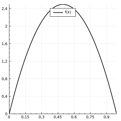
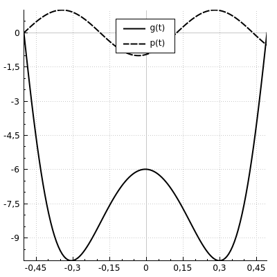
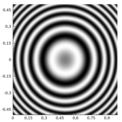
a)	b)	c)

Figure 1:  a) Initial condition $f\left(x\right).$ b) Boundary conditions $g\left(t\right)$ and $p\left(t\right)$. c) $F\left(x,t\right).$

Graphs of functions $F,f,g,p$ are presented on Figure 1. Thus, solving the forward problem (5.1)-(5.4) for the input functions (5.5)-(5.8), we have computed the function $q_{comp}\left(t\right),$

$$u_{x}\left(1,t\right)=q_{comp}\left(t\right),t\in\left(-1/2,1/2\right).$$ (5.9)

We now formulate precisely the ill-posed Cauchy problem which we have solved computationally.

Ill-Posed Cauchy Problem 2. Suppose that in (5.1)-(5.4) functions $f\left(x\right)$ and $g\left(t\right)$ are unknown whereas the functions $F\left(x,t\right)$ $p\left(t\right)$, $S\left(u\right)$ and the constant $a\geq 0$ are known. Suppose that in the data simulation process functions $F,S,f,g,p$ are the same as in (5.5)-(5.8). Determine the function $u\left(x,t\right)$ in at least a subdomain of the time cylinder $Q_{1/2}^{\pm}$ assuming that the function $q_{comp}\left(t\right)$ in (5.9) is known.

We now briefly describe how did we solve the forward problem (5.1)-(5.4) numerically using FDM. Introduce the uniform mesh in the domain $Q_{1/2}^{\pm},$

$$\overline{M}=\left\{\left(x_{i},t_{j}\right):x_{i}=ih,t_{j}=-\frac{1}{2}+j\tau,i\in\left[0,N\right),j\in\left[0,M\right)\right\},$$

where $h=1/N$ and $\tau=1/M$ are grid step sizes in $x$ and $t$ directions respectively. We have used $N=32,M=128.$ For generic functions $f^{\left(1\right)}\left(x,t\right),f^{\left(2\right)}\left(x\right),f^{\left(3\right)}\left(t\right)$ denote $f_{ij}^{\left(1\right)}=f^{\left(1\right)}\left(x_{i},t_{j}\right),f_{i}^{\left(2\right)}=f^{\left(2\right)}\left(x_{i}\right),f_{j}^{\left(3\right)}=f^{\left(3\right)}\left(t_{j}\right).$ Let $\varphi_{ij}=aS\left(u_{ij}\right)+F_{ij}.$ We have solved the forward problem (5.1)-(5.4) using the implicit finite difference scheme,

$$\frac{u_{ij+1}-u_{ij}}{\tau}=\frac{1}{h^{2}}\left(u_{i-1j+1}-2u_{ij+1}+u_{i+1j+1}\right)+\varphi_{ij},i\in\left[1,N-1\right),j\in\left[0,M-1\right),$$

$$u_{i0}=f_{i},\text{ }u_{0j}=g_{j},u_{nj}=p_{j},i\in\left[0,N\right),j\in\left[0,M\right),$$

5.2 Specifying the functional $J_{\lambda,\beta}$

In the case of (5.1)-(5.9) the operator $A$ becomes

$$K\left(u\right)=u_{t}-u_{xx}-aS\left(u\right)-F\left(x,t\right).$$

And the functional $J_{\lambda,\beta}$ is

$$J_{\lambda,\beta}\left(u\right)=\mathop{\displaystyle\int}\limits_{-1/2}^{1/2}\mathop{\displaystyle\int}\limits_{0}^{1}\left[K\left(u\right)\right]^{2}\varphi_{\lambda}^{2}dxdt+\beta\left\|u\right\|_{H^{2}\left(Q_{1/2}^{\pm}\right)}^{2}.$$ (5.10)

We have dropped here the multiplier $e^{-2\lambda\left(\alpha_{0}+\varepsilon\right)}$ which was present in the original version (2.16). Indeed, we have used this multiplier above in order to allow the parameter $\beta$ to be less than $1$. However, we have discovered in our computations that the accuracy of results does not change much for $\beta$ varying in a large interval. The norm $\left\|u\right\|_{H^{2}\left(Q_{1/2}^{\pm}\right)}$ is taken instead of $\left\|u\right\|_{H^{3}\left(Q_{1/2}^{\pm}\right)}$ due to the convenience of computations. Note that since we do not use too many grid points when discretizing the functional $J_{\lambda,\beta}\left(u\right),$ then these two norms are basically equivalent in our computations, since all norms in a finite dimensional space are equivalent.

5.3 The discrete form of $J_{\lambda,\beta}$

In our computations we represent derivatives in (5.10) in the form of finite differences with $N=32,M=128$ and minimize the resulting functional with respect to values of the function $u$ at grid points. Discretizing integrals, we obtain the following discrete form $\hat{J}$ of the functional (5.10)

$$\hat{J}(\hat{u})=\frac{1}{NM}\Big{[}\sum\limits_{i=1}^{N-2}\sum\limits_{j=0}^{M-2}K_{ij}^{2}\varphi_{\lambda ij}^{2}+\beta\sum\limits_{i=1}^{N-2}\sum\limits_{j=1}^{M-2}Y_{ij}\Big{]},$$ (5.11)

where $\hat{u}=\{u_{00},u_{10},...,u_{kn},...,u_{N-1M-1}\}$ is the vector of values of the function $u$ at grid points. Here 

$$K_{ij}=\frac{u_{ij+1}-u_{ij}}{\tau}-\frac{u_{i-1j}-2u_{ij}+u_{i+1j}}{h^{2}}-aS\left(u_{ij}\right)-F_{ij},$$

$$Y_{ij}=u_{ij}^{2}+\frac{\left(u_{ij+1}-u_{ij}\right)^{2}}{\tau^{2}}+\frac{\left(u_{i+1j}-u_{ij}\right)^{2}}{h^{2}}$$ (5.12)

$$+\frac{\left(u_{ij-1}-2u_{ij}+u_{ij+1}\right)^{2}}{\tau^{4}}+\frac{\left(u_{i-1j}-2u_{ij}+u_{i+1j}\right)^{2}}{h^{4}}.$$

To apply the conjugate gradient method (GCM), it is convenient to use explicit formulae for the derivatives $\partial\hat{J}(\hat{u})/\partial u_{kn}.$ Using (5.11), we obtain for indexes $1\leq k\leq N-2,1\leq n\leq M-2$

$$\frac{\partial\hat{J}}{\partial u_{kn}}=\frac{2}{NM}\sum\limits_{i=1}^{N-2}\sum\limits_{j=0}^{M-2}\varphi_{ij}^{2}K_{ij}\frac{\partial K_{ij}}{\partial u_{kn}}+\frac{\beta}{NM}\sum\limits_{i=0}^{N-2}\sum\limits_{j=1}^{M-2}\frac{\partial Y_{ij}}{\partial u_{kn}}.$$ (5.13)

We calculate these derivatives only with respect to those parameters $u_{kn}$ which correspond to internal grid points, i.e. for above indices. We set

$$\frac{\partial\hat{J}}{\partial u_{0j}}=0,\frac{\partial\hat{J}}{\partial u_{i0}}=\frac{\partial\hat{J}}{\partial u_{iM-1}}=0.$$ (5.14)

Also, we set to zero partial derivatives of $\hat{J}$ with respect to $u_{N-1j}$ and $u_{N-2j}.$ This is because values of $u_{N-1j}$ and $u_{N-2j}$ are known, see (5.17) and (5.18). So,

$$\frac{\partial\hat{J}}{\partial u_{N-2j}}=\frac{\partial\hat{J}}{\partial u_{N-1j}}=0$$

To simplify notations, we omit here and below the subscript $\lambda$ in$\varphi_{ij}^{2}.$ Using (5.12), we obtain

$$\sum\limits_{i=1}^{N-2}\sum\limits_{j=0}^{M-2}\varphi_{ij}^{2}K_{ij}\frac{\partial K_{ij}}{\partial u_{kn}}=$$

$$\frac{2}{\tau}\left(\varphi_{kn-1}^{2}K_{kn-1}-\varphi_{kn}^{2}K_{kn}\right)-\frac{2}{h^{2}}\Big{(}\varphi_{k-1n}^{2}K_{k-1n}-2\varphi_{kn}^{2}K_{kn}+\varphi_{k+1n}^{2}K_{k+1n}\Big{)}$$ (5.15)

$$-2\varphi_{kn}^{2}K_{kn}^{2}S^{\prime}(u_{kn}),$$

where $S^{\prime}(u_{kn})$ is determined by the function $S(u)$ and can be calculated analytically. Next,

$$\sum\limits_{i=0}^{N-2}\sum\limits_{j=1}^{M-2}\frac{\partial Y_{ij}}{\partial u_{kn}}=$$

$$2u_{kn}+\frac{2}{\tau}\Big{(}Ut_{kn+1}-Ut_{kn}\Big{)}+\frac{2}{h}\Big{(}Ux_{k+1n}-Ux_{kn}\Big{)}+$$ (5.16)

$$+\frac{2}{\tau^{2}}\Big{(}Utt_{kn+1}-2Utt_{kn}+Utt_{kn-1}\Big{)}++\frac{2}{h^{2}}\Big{(}Uxx_{k+1n}-2Uxx_{kn}+Uxx_{k-1n}\Big{)},$$

where

$$Ut_{kn}=\left\{\begin{array}[]{c}\frac{1}{\tau}(u_{kn+1}-u_{kn})\quad\text{if}\quad n\in[0,M-1)\\ 0\quad\text{if}\quad n=M-1;\end{array}\right.$$

$$Ux_{kn}=\left\{\begin{array}[]{c}\frac{1}{h}(u_{k+1n}-u_{kn})\quad\text{if}\quad k\in[0,N-1)\\ 0\quad\text{if}\quad k=N-1;\end{array}\right.$$

$$Utt_{kn}=\left\{\begin{array}[]{c}\frac{1}{\tau^{2}}(u_{kn+1}-2u_{kn}+u_{kn-1})\quad\text{if}\quad n\in(0,M-1)\\ 0\quad\text{if}\quad n=0\quad\text{and}n=M-1;\end{array}\right.$$

$$Uxx_{kn}=\left\{\begin{array}[]{c}\frac{1}{h^{2}}(u_{k+1n}-2u_{kn}+u_{k-1n})\quad\text{if}\quad k\in(0,N-1)\\ 0\quad\text{if}\quad k=0\quad\text{and}k=N-1;\end{array}\right.$$

In (5.15) and (5.16) we use boundary conditions (5.4) and (5.9) at $x=1$ as

$$u_{N-1j}=p_{j},u_{N-2j}=p_{j}-hq_{comp,j}.$$ (5.17)

5.4 Some notes about noisy data and the conjugate gradient method

In all our numerical experiments $\beta=0.00063.$ As we have stated in subsection 5.2, we have observed in our computations that this parameter does not influence much our results. All results below are obtained for noisy data with 5% level of noise. Here is how we have introduced this noise. Let $\sigma\in\left[-1,1\right]$ be the random variable representing the white noise. Let $p^{\left(m\right)}=\max_{j}\left|p_{j}\right|$ and $q^{\left(m\right)}=\max_{j}\left|q_{comp,j}\right|.$ Then by (5.17) the noisy data, which we have used, were

$$\widetilde{u}_{N-1j}=p_{j}+0.05p^{\left(m\right)}\sigma_{j},\widetilde{u}_{N-2j}=p_{j}-h\left(q_{comp,j}+0.05q^{\left(m\right)}\sigma_{j}\right).$$ (5.18)

In all our numerical tests we have used in (5.11) $M=32,N=128$. Even though these numbers are the same as in the solution of the forward problem, the “inverse crime” was not committed since we have used noisy data and since we have used the minimization of the functional (5.11) rather than solving a forward problem again. To minimize the functional, we have used the unconstrained CGM. We arrange this method in such a way that boundary conditions (5.18) are kept to be satisfied on all iterations. So, we minimize the functional (5.11) with respect to numbers $\left\{u_{ij}\right\}_{\left(i,j\right)=\left(2,2\right)}^{\left(N-3,M-3\right)}.$ However, numbers $u_{N-1j},u_{N-2j}$ are kept as (5.18). As the starting vector $\left\{u_{ij}^{0}\right\}$ we take

$$u_{ij}^{0}=\left\{\begin{array}[]{c}0\text{ if }i\in\left[0,N-3\right],\\ \widetilde{u}_{N-2j}\text{ if }i=N-2,\\ \widetilde{u}_{N-1j}\text{ if }i=N-1.\end{array}\right.$$ (5.19)

Normally, for a quadratic functional this method reaches its minimum after $M\cdot N$ gradient steps with the automatic step choice. However, our computational experience tells us that we can obtain a better accuracy if using a small constant step in the GCM and a constant number of iterations. Thus, we have used the step size $\gamma=10^{-8}$ and 10,000 iterations of the GCM. It took 0.5 minutes of CPU Intel Core i7 to do these iterations.

6 Numerical Results

Let $u\left(x,t\right)$ be the numerical solution of the forward problem (5.1)-(5.3). Let $u_{\lambda\beta}\left(x,t\right)$ be the minimizer of the functional (5.11) which we have found via GCM. Of course, $u\left(x,t\right)$ and $u_{\lambda\beta}\left(x,t\right)$ here are discrete functions defined on the above grid and norms used below are discrete norms. For each $x$ from this grid we define the “line error” $E\left(x\right)$ as

$$E\left(x\right)=\frac{\left\|u_{\lambda\beta}\left(x,t\right)-u\left(x,t\right)\right\|_{L_{2}\left(-1/2,1/2\right)}}{\left\|u\left(x,t\right)\right\|_{L_{2}\left(-1/2,1/2\right)}}.$$ (6.1)

We evaluate how the line error changes with the change of $x$. Since our lateral data are given at $x=1$, it is anticipated that the function $E\left(x\right)$ should be decreasing.

We have tested three values of the parameter $\lambda:\lambda=0,3,4.$ We have found that $\lambda=4$ is the best choice, at least for those problems which we have studied. Also, we have tested two values of the parameter $a$ in (5.1): $a=0$ and $a=10$. The case $a=0$ corresponds to the linear problem and $a=10$ indicates the nonlinearity.

6.1 Graphs of line errors

Graphs of the line error are presented on Figure 2. Figure 2a corresponds to the linear case with $a=0$. Figures 2b and 2c with $a=10$ display the line errors for two above functions $S\left(u\right).$ Figure 2b is for $S\left(u\right)=\sin^{2}\left(u\right)$ and Figure 2c is for $S\left(u\right)=\exp\left(0.4u\right).$ One can observe that for both values $\lambda=3$ and $\lambda=4$ all three cases have an acceptable error up to $x=0.45.$ In other words, the function $u\left(x,t\right)$ is reconstructed rather accurately on more than half of the interval $\left[0,1\right]$: for $x\in\left[0.45,1\right].$ Thus, in all cases the presence of the CWF significantly improves the accuracy of the solution. Furthermore, the presence of the CWF improves the accuracy even in the linear case.

The case $a=0,\lambda=0$ corresponds to the Quasi-Reversibility Method, which was first introduced by Lattes and Lions [28]. This method works only for linear PDEs. The convergence rate of this method can be established via Carleman estimates, see [4, 5, 7, 8, 20] and the recent survey [23].

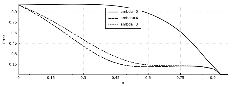
a)

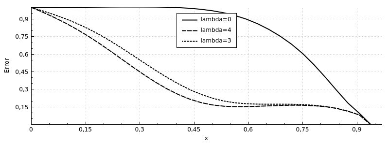
b)

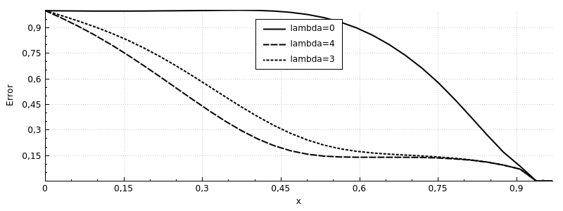
c)

Figure 2: Line errors. a) The linear problem with $a=0$ for $\lambda=0,3,4.$ The case $a=0,\lambda=0$ corresponds to the Quasi-Reversibility Method. b) $a=10,\lambda=0,3,4$ and $S\left(u\right)=\sin^{2}\left(u\right).$ c) $a=10,\lambda=0,3,4$ and $S\left(u\right)=\exp\left(0.4u\right).$ Thus, in all cases the presence of the CWF in the functional (5.11) significantly improves the accuracy of the solution. Furthermore, the presence of the CWF improves the accuracy even in the linear case. In all cases a rather accurate reconstruction is obtained for $x\in\left[0.45,1\right],$ i.e. on more than half of the interval $\left[0,1\right].$

6.2 Graphs of functions $u_{\lambda\beta}\left(0.6,t\right)$

As one can see on Figures 2 a)-c), the line error at $x=0.6$ is about 10% for $\lambda=0,4$ for all three cases. Thus, we have decided to superimpose graphs of functions $u_{\lambda\beta}\left(0.6,t\right)$ with graphs of functions $u\left(0.6,t\right).$ One can see on Figures 3a)-c) that graphs of functions $u_{0\beta}\left(0.6,t\right)$ are rather far from the graph of functions $u\left(0.6,t\right).$ On the other hand, the presence of the CWF in the functional (5.11) makes graphs of functions $u_{4\beta}\left(0.6,t\right)$ to be quite close to the graph functions $u\left(0.6,t\right).$ This is true even for the linear case of Figure 3a). On the other hand, functions $u_{0\beta}\left(0.6,t\right)$ and $u_{4\beta}\left(0.6,t\right)$ drop to zero as $t\rightarrow-1/2^{+}.$ Also, the accuracy at $t\approx 1/2$ is not good on Figures 3a),b). We explain this by condition (5.14) which we have imposed. In addition, in the accuracy estimates (2.25), (2.26) $G_{\alpha_{0}+2\varepsilon}\cap\left\{t=\pm 1/2\right\}=\varnothing.$

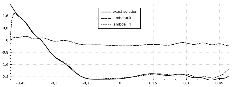
a)

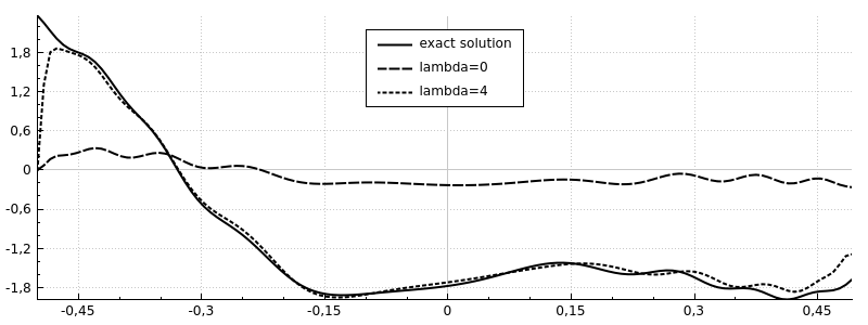
b)

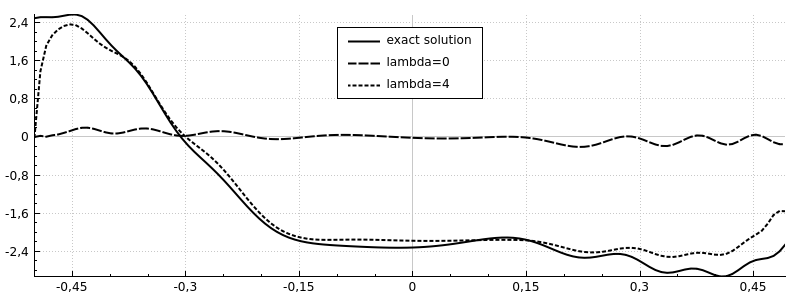
c)

Figure 3: Superimposed graphs of functions $u_{0\beta}\left(0.6,t\right),u_{4\beta}\left(0.6,t\right)$ and $u\left(0.6,t\right).$ a) The linear case, $a=0$. b) $a=10,S\left(u\right)=\sin^{2}\left(u\right).$ c) $a=10,S\left(u\right)=\exp\left(0.4u\right).$ Observe that the presence of the CWF with $\lambda=4$ quite essentially improves the accuracy of the solution in all three cases, including even the linear case.

6.3 The influence of the initial condition

To see how the knowledge of the initial condition $u\left(x,-1/2\right)=f\left(x\right)$ affects the accuracy of our results, we have tested the case when the function $f\left(x\right)$ in (5.7) is known. Now we arrange the GCM in such a way that both boundary conditions (5.18) and the initial condition $u_{i0}=f_{i}$ are kept be satisfied on all iterations. Similarly with (5.19) the first guess $\left\{u_{ij}^{0}\right\}$ is taken as

$$u_{ij}^{0}=\left\{\begin{array}[]{c}0\text{ if }i\in\left[0,N-3\right],j\neq 0,\\ \widetilde{u}_{N-2j}\text{ if }i=N-2,j\neq 0,\\ \widetilde{u}_{N-1j}\text{ if }i=N-1,j\neq 0,\\ f_{i}\text{ if }j=0.\end{array}\right.$$

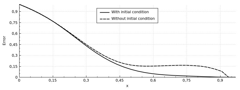
a)

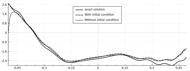
b)

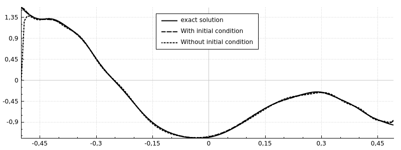
c)

Figure 4: The influence of the knowledge of the initial condition. The case $a=10,S\left(u\right)=exp(0.4u)\left(u\right).$ a) Line errors. b) Graphs of functions $u_{4\beta}\left(0.6,t\right)$ with and without knowledge of the initial condition, superimposed with the graph of the function $u\left(0.6,t\right).$ c) The same as in b) but for functions $u_{4\beta}\left(0.8,t\right),u\left(0.8,t\right).$ One can see that the knowledge of the initial condition does not provide an essential impact in the accuracy of the solution.

Here we consider the case $a=10,S\left(u\right)=\sin^{2}\left(u\right).$ Figure 4a) displays the line errors with and without knowledge of the function $f\left(x\right)$ in (5.7). One can see that for $x\in\left[0.45,1\right]$ the error for the case when $f\left(x\right)$ is known is less than for the case when $f\left(x\right)$ is unknown. Figure 4b) displays graphs of functions $u_{4\beta}\left(0.6,t\right)$ for the cases of known and unknown initial condition. They are superimposed with the graph of the function $u\left(0.6,t\right).$ One can observe that these three graphs are only slightly different from each other on the major part of the time interval.  Figure 4c) displays graphs of functions $u_{4\beta}\left(0.8,t\right)$ for the cases of known and unknown initial condition. They are superimposed with the graph of the function $u\left(0.8,t\right).$ One can see that these graphs almost coincide, except of $t\approx-1/2.$ Thus, the knowledge of the initial condition does not provide an essential impact in the accuracy of the solution.

Acknowledgments

The work of the first author was supported by US Army Research Laboratory and US Army Research Office grant W911NF-15-1-0233 and by the Office of Naval Research grant N00014-15-1-2330.

References

- [1] Andrieux S and Baranger T N 2015 Solution of nonlinear Cauchy problem for hyperelastic solids Inverse Problems 31 115003.
- [2] Beilina L and Klibanov M V 2012 Approximate Global Convergence and Adaptivity for Coefficient Inverse Problems, Springer, New York.
- [3] Beilina L and Klibanov M V 2015 Globally strongly convex cost functional for a coefficient inverse problem Non Linear Analysis: Real World Applications 22 272-288.
- [4] Becache E, Bourgeois L Franceschini L and Dardé J 2015 Application of mixed formulations of quasi-reversibility to solve ill-posed problems for heat and wave equations: the 1D case Inverse Problems and Imaging 9 971-1002.
- [5] Bourgeois L and J. Dardé J 2010, A quasi-reversibility approach to solve the inverse obstacle problem, Inverse Problems and Imaging 4 351-377.
- [6] Bukhgeim A L and M.V. Klibanov M V 1981 Uniqueness in the large of a class of multidimensional inverse problems Soviet Mathematics Doklady 17 244-247.
- [7] Dardé J, Hannukainen A, Hyvönen N 2013 An based mixed quasi-reversibility method for solving elliptic Cauchy problems SIAM J. Numer. Anal. 51 2123-2148.
- [8] Dardé J 2015 Iterated quasi-reversibility method applied to elliptic and parabolic data completion problems arxiv 1503.08641.
- [9] Eldén L 1995 Numerical solution of the sideways heat equation by difference approximation in time, Inverse Problems 11 913-923.
- [10] Eldén L, Berntsson F and Regińska T 2000 Wavelet and Fourier methods for solving the sideways heat equation, SIAM J. Sci. Comput. 21 2187-2205.
- [11] Hào D N and Lesnic D 2000 The Cauchy problem for Laplace’s equation via the conjugate gradient method IMA J. Appl. Math. 65 199-217.
- [12] Imanuvilov O Yu and M. Yamamoto M 2001 Global uniqueness and stability in determining coefficients of wave equations, Commun. in Partial Differential Equations 26 1409-1425.
- [13] Imanuvilov O Yu and Yamamoto M 2001 Global Lipschitz stability in an inverse hyperbolic problem by interior observations Inverse Problems 17 717-728.
- [14] Isakov V 2004 Carleman estimates and applications to inverse problems, Milan J. of Mathematics 72 249-271.
- [15] Isakov V 2006 Inverse Problems for Partial Differential Equations, Second Edition, Springer, New York.
- [16] Kabanikhin S I 2012 Inverse and Ill-Posed Problems Walter de Gruyter GmbH & Co. KG, Berlin.
- [17] Kabanikhin S I and Karchevsky A L 1995 Optimizational method for solving the Cauchy problem for an elliptic equation J. Inverse and Ill-Posed Problems 3 21-46.
- [18] Karchevsky A L, Marchuk I V and Kabov O A 2016 Calculation of the heat flux near the liquid–gas–solid contact line Applied Mathematical Modeling 40 1029-1037.
- [19] Klibanov M V 1997 Global convexity in a three-dimensional inverse acoustic problem, SIAM J. Math. Anal. 28 1371-1388.
- [20] Klibanov M and Timonov A 2004 Carleman Estimates for Coefficient Inverse Problems and Numerical Applications VSP, Utrecht, The Netherlands.
- [21] Klibanov M 2013 Carleman estimates for global uniqueness, stability and numerical methods for coe cient inverse problems J. Inverse Ill-Posed Problems 21 477-560.
- [22] Klibanov M V and Thành N T 2015 Recovering of dielectric constants of explosives via a globally strictly convex cost functional, SIAM J. Appl. Math. 75 518-537.
- [23] Klibanov M V 2015 Carleman estimates for the regularization of ill-posed Cauchy problems, Applied Numerical Mathematics 94 46-74.
- [24] Klibanov M V 2015 Carleman weight functions for solving ill-posed Cauchy problems for quasilinear PDEs Inverse Problems 31 125007.
- [25] Klibanov M V and Kamburg V G 2016 Globally strictly convex cost functional for an inverse parabolic problem Mathematical Methods in the Applied Sciences 39 930-940.
- [26] Berntsson F, V.A. Kozlov V A, Mpinganzima L and B.O. Turesson B O 2014 An alternating iterative procedure for the Cauchy problem for the Helmholtz equation, Inverse Problems in Science and Engineering 22 45–62.
- [27] Ladyzhenskaya O A, Solonnikov V A and Ural’ceva N N 1968 Linear and Quasilinear Equations of Parabolic Type AMS, Providence, R.I.
- [28] R. Lattes and J.-L. Lions, The Method of Quasireversibility: Applications to Partial Differential Equations, Elsevier, New York, 1969.
- [29] Lavrentiev M M, Romanov V G and Shishatskii S P 1986 Ill-Posed Problems of Mathematical Physics and Analysis (Providence, RI: AMS).
- [30] Rischette R, Baranger T N and Debit N 2014 Numerical analysis of an energy-like minimization method to solve a parabolic Cauchy problem with noisy data J. Computational and Applied Mathematics 271 206-222.
- [31] Tikhonov A N, Goncharsky A V, Stepanov V V and Yagola A G 1995 Numerical Methods for the Solution of Ill-Posed Problems (London: Kluwer).
- [32] Triggiani R and Zhang Z 2015 Global uniqueness and stability in determining the electric potential coefficient of an inverse problem for Schrödinger equations on Riemannian manifolds J. Inverse and Ill-Posed Problems 23 587-609
- [33] Yamamoto M 2009 Carleman estimates for parabolic equations and applications. Topical Review. Inverse Problems 25 123013.