Shortest Paths and Convex Hulls in 2D Complexes with Non-Positive Curvature

Abstract

Globally non-positively curved, or CAT(0), polyhedral complexes arise in a number of applications, including evolutionary biology and robotics. These spaces have unique shortest paths and are composed of Euclidean polyhedra, yet many algorithms and properties of shortest paths and convex hulls in Euclidean space fail to transfer over. We give an algorithm, using linear programming, to compute the convex hull of a set of points in a 2-dimensional CAT(0) polyhedral complex with a single vertex. We explore the use of shortest path maps to answer single-source shortest path queries in 2-dimensional CAT(0) polyhedral complexes, and we unify efficient solutions for 2-manifold and rectangular cases.

1 Introduction

Convex hulls and shortest paths—and algorithms to find them—are very well understood in Euclidean spaces, but less so in non-Euclidean spaces. We consider these two problems in finite polyhedral complexes which are formed by joining a finite number of $d$-dimensional convex polyhedra along lower dimensional faces. We will primarily be concerned with the 2D case of triangles or rectangles joined at edges.

We will restrict our attention to polyhedral complexes that are globally non-positively curved, or CAT(0). Introduced by Gromov in 1987 [29], CAT(0) metric spaces (or spaces of global non-positive curvature) constitute a far-reaching common generalization of Euclidean spaces, hyperbolic spaces and simple polygons. The initials “CAT” stand for Cartan, Alexandrov, and Toponogov, three researchers who made substantial contributions to the theory of comparison geometry. In a CAT(0) space, in contrast to a space of positive curvature, there is a unique geodesic (locally shortest path) between any two points and this property characterizes CAT(0) complexes.

The impact of CAT(0) geometry on mathematics is significant especially in the field of geometric group theory where the particular case of CAT(0) polyhedral complexes formed by cubes—the so-called “CAT(0) cube complexes”—are particularly relevant [1, 32, 55]. Most of the work on CAT(0) metric spaces so far has been mathematical. Algorithmic aspects remain relatively unexplored apart from a few results for some particular CAT(0) spaces [20, 21, 25, 44].

This paper is about algorithms for finite CAT(0) polyhedral complexes, which we will call “CAT(0) complexes” from now on. We are primarily interested in the algorithmic properties of CAT(0) complexes because of their applications, particularly to computational evolutionary biology. The (moduli) space of all phylogenetic (evolutionary) trees with $n$ leaves can be modelled as a CAT(0) cube complex with a single vertex [11], and being able to compute convex hulls in this space would give a method for computing confidence intervals for sets of trees (see Section 2.3 for more details). A second application of CAT(0) cube complexes is to reconfigurable systems [28], a large family of systems which change according to some local rules, e.g. robotic motion planning, the motion of non-colliding particles in a graph, and phylogenetic tree mutation, etc. In many reconfigurable systems, the parameter space of all possible positions of the system can be seen as a CAT(0) cube complex [28]. CAT(0) cube complexes are also in bijection with median graphs [20], which have been applied to phylogenetics [4] as well, and with domains of event structures [7].

Main Results. In this paper we study the shortest path problem and the convex hull problem in 2D CAT(0) complexes formed by triangles or rectangles. For any set of points $P$ we define the convex hull to be the minimal set containing $P$ that is closed under taking the shortest path between any two points in the set. We show that convex hulls in 2D CAT(0) complexes fail to satisfy some of the properties we take for granted in Euclidean spaces. Our main result is an algorithm to find the convex hull of a finite set of points in a 2D CAT(0) complex with a single vertex. In general, for any CAT(0) complex, the convex hull of a set of points is the union of a convex set in each cell of the complex. For the case of 2D CAT(0) complexes, these convex sets are polygons which may be open or closed on parts of their boundaries. For the special case when there is a single vertex, we show how to find these polygons using linear programming. Our algorithm runs in polynomial time (in bit complexity) for a cube complex. For more general inputs we must use the real-RAM model of computation, and the bottleneck in our running time is the time required for linear programming in an algebraic model, which is not known to be polynomially bounded, but is considered efficient via the simplex method.

In the single-source shortest path problem, we are given a 2D CAT(0) complex of $n$ triangles and a source point $s$, and we wish to preprocess the complex in order to find the shortest path from $s$ to any query point $t$ quickly. We explore the shortest path map, which divides the space into regions where shortest paths from $s$ are combinatorially the same (i.e. traverse the same sequence of edges and faces). We show that the shortest path map may have exponential size. An alternative, the “last step shortest path map,” has linear size and can be used to find shortest paths from $s$ in time proportional to the number of faces traversed by the path. We show how to construct the last step shortest path map in $O(n^{2})$ preprocessing time and space for special cases. This generalizes and unifies two previous results: an algorithm by Chepoi and Maftuleac [22] for the case of 2D CAT(0) rectangular complexes; and an algorithm by Chen and Han [19] specialized to the case of a 2D CAT(0) complex that is a topological 2-manifold with boundary (i.e. every edge is incident to at most two faces).

The rest of the paper is organized as follows. Section 2 contains further background on the problem, including existing algorithmic results for CAT(0) polyhedral complexes and applications to phylogenetics. Section 3 reviews the relevant mathematics and tree space notation. Section 4 gives our results for convex hulls, and Section 5 gives our results for shortest paths in 2D CAT(0) polyhedral complexes. Finally we give our conclusions in Section 6.

2 Background

In this section we describe background work on shortest path and convex hull algorithms, and discuss the application of our work to phylogenetic trees.

One of the most basic CAT(0) spaces is any simple polygon (interior plus boundary) in the plane. This can be viewed as a 2D CAT(0) complex once the polygon is triangulated. The fact that geodesic paths are unique is at the heart of efficient algorithms for shortest paths and related problems. On the other hand, generalizing a polygon to a polygonal domain (a polygon with holes) or a polyhedral terrain yields spaces that are not CAT(0), since geodesic paths are no longer unique. This helps explain why shortest path and convex hull problems are more difficult in these more general settings.

2.1 Shortest Paths

The shortest path problem is a fundamental algorithmic problem with many applications, both in discrete settings like graphs and networks (see, e.g., [2]) as well as in geometric settings like polygons, polyhedral surfaces, or 3-dimensional space with obstacles (see, e.g., Mitchell [46]).

All variants of the shortest path problem can be solved efficiently for a polygon once it is triangulated, and triangulation can be done in linear time with Chazelle’s algorithm [17]. The shortest path (the unique geodesic) between two given points can be found in linear time [41]. For query versions, linear space and linear preprocessing time allow us to answer single-source queries [30, 34], and more general all-pairs queries [31], where answering a query means returning the distance in logarithmic time, and the actual path in time proportional to its number of edges.

By contrast, in a polygonal domain, where geodesic paths are no longer unique, the best single-source shortest path algorithm uses a continuous-Dijkstra approach in which paths are explored by order of distance. For a polygonal domain of $n$ vertices, this method takes $O(n\log n)$ [preprocessing] time [35] (see the survey by Mitchell [46]). For a polyhedral terrain the continuous-Dijkstra approach gives $O(n^{2}\log n)$ time [47], and the best-known run-time of $O(n^{2})$ is achieved by Chen and Han’s algorithm [19] that uses a breadth-first-search approach.

There are no shortest path algorithms for the general setting of CAT(0) polyhedral complexes, although there are some for certain specializations. For 2D CAT(0) complexes that are 2-manifolds, the algorithm of Chen and Han [19] applies (in fact, they do not need the CAT(0) property), and solves the single-source shortest path problem with preprocessing time $O(n^{2})$, space $O(n)$ and query time (to produce the path) proportional to the size of the output path. Maftuleac [44] explicitly discussed this as a problem in a CAT(0) space and gave a Dijkstra-like algorithm with the same space and query time, but preprocessing time of $O(n^{2}\log n)$. Chepoi and Maftuleac [22] used different methods to give a polynomial time algorithm for all-pair shortest path queries in any 2D CAT(0) rectangular complex, with preprocessing time $O(n^{2})$, space $O(n^{2})$, and query time proportional to the size of the output path.

There are also some results on finding shortest paths when we restrict the CAT(0) polyhedral complex to be composed of cubes or rectangles. The space of phylogenetic trees mentioned in the introduction is a special type of CAT(0) cube complex. For these “tree spaces,” Owen and Provan [53] gave an algorithm to compute shortest paths (geodesics) with a running time of $O(d^{4})$, where $d$ is the dimension of the maximal cubes. The algorithm is much faster in practice for realistic phylogenetic trees. The result was extended to a polynomial time algorithm for computing geodesics in any orthant space [45], where an orthant space is a CAT(0) cube complex with a single vertex. Very recently, Hayashi [33] gave a polynomial time algorithm to compute approximate shortest paths in a general CAT(0) cube complex. In fact, his algorithm will be polynomial time in any CAT(0) space in which certain conditions are met, mainly being able to compute shortest paths between any pair of points within a fixed distance $D$ of each other in polynomial time, and having an initial path that consists of a sequence of shortest paths, each of length less than $D$. It is not clear how to meet his preconditions in a 2D CAT(0) complex. It is not possible to compute exact shortest paths in CAT(0) cube complexes of dimension three or more because Ardila et al. [3] showed that, in general, the coordinates of the points where geodesics crosses orthant boundaries are the solutions to higher ordered algebraic equations, and thus cannot be expressed by closed form formulas.

2.2 Convex Hulls

The problem of computing the convex hull of a set of points is fundamental to geometric computing, especially because of the connection to Voronoi diagrams and Delaunay triangulations [42].

The convex hull of a set of points in the plane can be found in provably optimal time $O(n\log h)$ where $n$ is the number of points and $h$ is the number of points on the convex hull. The first such algorithm was developed by Kirkpatrick and Seidel [40] and a simpler algorithm was given by Chan [16]. An optimal algorithm for computing convex hulls in higher dimension $d$ in time $O(n^{\lfloor\frac{d}{2}\rfloor})$ was given by Chazelle [18]. See the survey by Seidel [56].

A simple polygon, triangulated by chords, is the most basic example of a 2D CAT(0) complex. In this setting, the convex hull of a set of points $P$ (i.e. the smallest set containing $P$ and closed under taking geodesics) is referred to as the relative (or geodesic) convex hull. Toussaint gave an $O(n\log n)$ time algorithm to compute the relative convex hull of a set of points in a simple polygon [57], and studied properties of such convex hulls [58]. Ishaque and Tóth [37] considered the case of line segments that separate the plane into simply connected regions (thus forming a CAT(0) space) and gave an semi-dynamic algorithm to maintain the convex hull of a set of points as line segments are added and points are deleted.

Moving beyond polygons to polygonal domains or terrains, geodesic paths are no longer unique, so there is no single natural definition of convex hull (one could take the closure under geodesic paths, or the closure under shortest paths). We are unaware of algorithmic work on these variants.

However, in a polyhedral surface with unique geodesics the convex hull is well defined, and Maftuleac [44] gave an algorithm to compute the convex hull of a set of points in $O(n^{2}\log n)$ time, where $n$ is the number of vertices in the complex plus the number of points in the set.

In all the above cases the boundary of the convex hull is composed of segments of shortest paths between the given points, which—as we shall see in Section 4.2—is not true in our setting of 2D CAT(0) complexes.

Beyond polyhedral complexes, convex hulls become much more complicated. Indeed it is still an open question if the convex hull of 3 points on a general Riemannian manifold of dimension 3 or higher is closed [10, Note 27]. Bowditch [13] and Borbély [12] give some results for convex hulls on manifolds of pinched negative curvature, but our complexes need not be manifolds. In the space of positive definite matrices, which is a CAT(0) Riemannian manifold, Fletcher et al. [27] give an algorithm to compute generalized convex hulls using horoballs, which are generalized half-spaces. Lin et al. [43] look at convex hulls of three points in an orthant space. They prove that there are such spaces where the top-dimensional cells have dimension $2d$, and there exist 3 points in the space such that their convex hull contains a $d$-dimensional simplex. Bridson and Haefliger [14, Proposition II.2.9] give conditions for when the convex hull of three points in a CAT(0) space is “flat”, or 2-dimensional. Finally, for a survey of convexity results in complete CAT(0) (aka Hadamard) spaces, of which the space of phylogenetic trees is one, see [9]. As an alternative to geodesically closed convex hulls in CAT(0) orthant spaces, Nye et al. [51] propose the locus of the Fréchet mean, which generalizes the Euclidean definition of a convex hull as a weighted combination of points.

2.3 Application to phylogenetic trees

While this paper will look at arbitrary 2D complexes with non-positive curvature, our work is motivated by a particular complex with non-positive curvature, namely the space of phylogenetic trees introduced by Billera, Holmes, and Vogtmann [11], called the BHV tree space, and described in more detail in Section 3.1. Phylogenetic trees are ubiquitous in biology, and each one depicts a possible evolutionary history of a set of organisms, represented as the tree’s leaves. Once we fix a set of leaves, the BHV tree space is a complex of Euclidean orthants (the higher dimensional version of quadrants and octants), in which each point in the space represents a different phylogenetic tree on exactly that set of leaves.

One area of active phylogenetics research is how to statistically analyze sets of phylogenetic trees on the same, or roughly the same, set of species. Such sets can arise in various ways: from sampling a known distribution of trees, such as that generated by the Yule process [61]; from tree inference programs, such as the posterior distribution returned by performing Bayesian inference [54] or the bootstrap trees from conducting a maximum likelihood search [26]; or from improvements in genetic sequencing technologies that lead to large sets of gene trees, each of which represents the evolutionary history of a single gene, as opposed to the species’ evolutionary history as a whole. Traditionally, most of the research in this area focused on summarizing the set of trees, although recent work has included computing variance [8, 45] and principal components [50].

It is an open question to find a good way to compute confidence regions for a set of phylogenetic trees. Willis [60] recently proposed a method for constructing confidence sets based on the Central Limit Theorem for BHV tree space [6, 5]. An alternative, non-parametric approach was proposed by Holmes [36], who suggested applying the data depth approach of peeling convex hulls for Euclidean space [59] to the BHV tree space. The convex hull is the minimum set that contains all the data points, as well as all geodesics between points in the convex hull. By peeling convex hulls, we mean to compute the convex hull for the data set, and then remove all data points that lie on the convex hull. This can then be repeated. To get the 95% confidence region, for example, one would remove successive convex hulls until only 95% of the original data points remain.

If we keep peeling convex hulls until all remaining points lie on the boundary of the convex hull, then we can take their Fréchet mean [8, 45] to get an analog of the univariate median of Tukey [59]. This could also be a useful one-dimensional summary statistic for a set of trees. Many of the most-used tree summary statistics have a tendency to yield a degenerate or non-binary tree, which is a tree in which some of the ancestor relationships are undefined. This is considered a problem by biologists, but such a univariate median tree found by peeling convex hulls would likely be binary if all trees in the data set are.

Currently, these methods cannot be used, because it is not known how to compute convex hulls in BHV tree space. We show several examples of how Euclidean intuition and properties for convex hulls do not carry over to convex hulls in the BHV tree space. Our algorithm to find convex hulls applies to the space of trees with five leaves which is described in more detail in Section 3.1.

3 Preliminaries

A metric space $(X,d)$ is geodesic if every two points $x,y\in X$ are connected by a locally shortest or geodesic path. A geodesic metric space $X$ is CAT(0) if its triangles satisfy the following CAT(0) inequality. For any triangle $ABC$ in $X$ with geodesic segments for its sides, construct a comparison triangle $A^{\prime}B^{\prime}C^{\prime}$ in the Euclidean plane such $d(A,B)={|A^{\prime}B^{\prime}|}$, $d(A,C)={|A^{\prime}C^{\prime}|}$, and $d(B,C)={|B^{\prime}C^{\prime}|}$. Let $Y$ be a point on the geodesic between $B$ and $C$, and let $Y^{\prime}$ be a comparison point on the line between $B^{\prime}$ and $C^{\prime}$ such that $d(B,Y)={|B^{\prime}Y^{\prime}|}$. Then triangle $ABC$ satisfies the CAT(0) inequality if $d(Y,A)\leq{|Y^{\prime}A^{\prime}|}$ for any $Y$. Intuitively, this corresponds to all triangles in $X$ being at least as skinny as the corresponding triangle in Euclidean space (Figure 1).

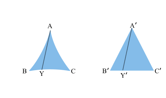
Figure 1: The triangle on the left represents a triangle in a CAT(0) space, with its corresponding comparison triangle in Euclidean space on the right.

A polyhedral complex is a set of convex polyhedra (“cells”) glued together by isometries along their faces. In this paper we only consider finite polyhedral complexes. When all of the cells are cubes, then this is called a cube, or cubical, complex. The length of a path between two points in a polyhedral complex is the sum of the Euclidean lengths of the pieces of the path in each cell of the complex. The distance between two points is defined as the length of the shortest path between them.

We will consider polyhedral complexes that are CAT(0). The cells are 2D (planar) convex polygons. These can always be triangulated, so the general setting is when the cells are triangles. We call this a 2D CAT(0) complex. Sometimes we will consider a complex in which all the cells are rectangles, either bounded or unbounded. We call this a 2D CAT(0) rectangular complex. In general we allow the space to have boundary (i.e., an edge that is incident to only one cell).

A 2D CAT(0) complex can be specified by giving its combinatorial information (the list of vertices, edges, and cells together with their incidence relationships) and the geometry of each cell. Each cell is a convex polygon that can be given either in local coordinates, or as angles and edge lengths. Converting between these two representations requires a real RAM model of computation in general, though for rectangular complexes, the conversion is efficient as measured by bit complexity, since all angles are $90^{\circ}$.

If a geodesic path in a 2D CAT(0) complex travels through a sequence of cells, we can “unfold” the cells into the plane where the path becomes a straight line. This result, and its history, is thoroughly discussed by Mitchell et al. [48], for the case of a 2-manifold (a polyhedral surface). The same is true in general 2D CAT(0) complexes since a geodesic path can never revisit an edge, i.e., the sequence of cells traversed by a geodesic path forms a 2-manifold.

For any vertex $v$ of a 2D complex, we define the link graph, $G_{v}$ as follows. The vertices of $G_{v}$ correspond to the edges incident to $v$ in the complex. The edges of $G_{v}$ correspond to the cells incident to $v$ in the complex: if $r$ and $s$ are edges of cell $C$ with $r$ and $s$ incident to $v$, then we add an edge between vertices $r$ and $s$ in $G_{v}$ with weight equal to the angle between $r$ and $s$ in $C$. Every point $p\neq v$ in cell $C$ can be mapped to a point on edge $(r,s)$ in $G_{v}$: if the angle between $vr$ and $vp$ in $C$ is $\alpha$ then $p$ corresponds to the point along edge $(r,s)$ that is distance $\alpha$ from $r$.

When we have a 2D polyhedral complex, there is also an alternative condition for determining whether it is CAT(0).

Theorem 1 ([14, Theorem II.5.4 and Lemma II.5.6]).

A 2D polyhedral complex $\cal K$ is CAT(0) if and only if it is simply connected and for every vertex $v\in{\cal K}$, every cycle in the link graph $G_{v}$ has length at least $2\pi$.

Some of our results are only for the case where the CAT(0) complex $\cal K$ has a single vertex $O$, which we call the origin. We will call such a complex a single-vertex complex. In a 2D single-vertex complex every cell is a cone formed by two edges incident to $O$ with angle at most $\pi$ between them. There is a single link graph $G=G_{O}$. Every point $p$ of the complex except $O$ corresponds to a point $\lambda(p)$ of $G$, and every point of $G$ corresponds to a ray of points in the complex.

3.1 BHV Tree Space

As explained in Section 2.3 the work on computing convex hulls was motivated by the BHV tree space for trees with 5 leaves, which is a 2D CAT(0) complex. We will now describe this space, which is denoted $\mathcal{T}_{5}$, and which contains all unrooted leaf-labelled, edge-weighted phylogenetic trees with 5 leaves (equivalently all such rooted trees with 4 leaves). For a description of the BHV tree spaces for trees with more than 5 leaves, see [11]. This section is not necessary for understanding the rest of the paper.

A phylogenetic tree is a tree in which each interior vertex has degree $\geq 3$ and there is a one-to-one labelling between the leaves (degree 1 vertices) and some set of labels $\cal L$. For this paper, we assume ${\cal L}=\{1,2,3,4,5\}$. Also, the trees have a positive weight or length on each interior edge, which is an edge whose vertices have degree $\geq 3$ (that is, are not leaves). If a phylogenetic tree contains only vertices of degree 1 and 3, then it is called binary.

Figure 2: Several tree shapes with their constituent splits listed below them. Tree (a) and tree (b) have the same tree shape, which does not depend on the planar embedding of the tree. Tree (c) has different splits and hence a different tree shape from trees (a) and (b). Tree (d) is a non-binary tree shape.

A split is a partition of the leaf-set $\cal L$ into two parts $L_{1}\cup L_{2}=\cal L$ such that $|L_{i}|\geq 2$ for $i=1,2$. We write a split as $L_{1}|L_{2}$. Each interior edge in a phylogenetic tree corresponds to a unique split, where the two parts are the sets of leaves in the two subtrees formed by removing that edge from the tree. Binary trees with five leaves contain two interior edges, and hence two splits. There are 10 possible splits, and they can be combined to form 15 different tree shapes. The shape of a tree is defined to be the set of interior edges or splits in that tree, and tell us which species are most closely related. (Figure 2).

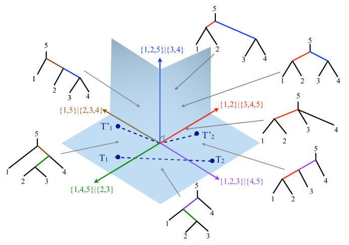
Figure 3: Five quadrants in $\mathcal{T}_{5}$. The upper right quadrant illustrates how trees with the same tree shape but different edge lengths lie at different coordinates in the quadrant. The dashed lines represent geodesics between two pairs of trees where $T_{i}$ and $T_{i}^{\prime}$ have the same tree shape but different edges lengths. The geodesic $T_{1}^{\prime}$ to $T_{2}^{\prime}$ passes through the origin, while the geodesic $T_{1}$ to $T_{2}$ passes through an intermediate quadrant.

We now define the space $\mathcal{T}_{5}$ itself, which consists of exactly one Euclidean quadrant for each of the 15 possible binary tree shapes. For each quadrant, the two axes are labelled by the two splits in the tree shape. A point in the quadrant corresponds to the tree with that tree shape whose interior edges have the lengths given by the coordinates. We identify axes labelled by the same split, so that if two quadrants both contain an axis labelled by the same split, then they are glued together along that shared axis (see Figure 3).

The length of a path between two trees in $\mathcal{T}_{5}$ is the sum of the lengths of the restriction of that path to each quadrant in turn, where it is computed using the Euclidean metric. The BHV distance is the length of the shortest path, or geodesic, between the two trees (Figure 3). Billera et al. [11] proved that this tree space is a CAT(0) cube complex, which implies that there is a unique geodesic between any two trees in the tree space.

To understand how the 15 quadrants in $\mathcal{T}_{5}$ are connected, consider the link graph of the origin, which is shown in Figure 4 and is the Petersen graph. The Petersen graph has multiple overlapping 5-cycles, one of which corresponds to the 5 quadrants in Figure 3. Also note that each vertex in the link graph of the origin is incident to three edges. This corresponds to each axis lying in three quadrants in $\mathcal{T}_{5}$. Note that this example illustrates that the link graph of even a CAT(0) rectangular complex with a single vertex need not be planar.

Figure 4: The Petersen graph, which is the link graph of the origin of $\mathcal{T}_{5}$. The graph edges correspond to tree shapes, and the graph vertices correspond to splits. The 5 quadrants in Figure 3 correspond to the outer 5-cycle in the Petersen graph.

4 Convex Hulls

Let $P$ be a finite set of points in a CAT(0) complex $\cal K$. Recall from Section 1 that the convex hull of $P$ is defined to be the minimal set containing $P$ that is closed under taking the shortest path between any two points in the set. Let CH$(P)$ denote the convex hull of $P$ in $\cal K$. For algorithmic purposes, there are several ways to specify CH$(P)$. One possibility is to specify the intersection of CH$(P)$ with each cell of the complex. In the case of 2D CAT(0) complexes, each such set is a convex polygon which may be open or closed on parts of its boundary. Our algorithm finds the vertices of each such polygon, and thus finds the closure of ${\rm CH}(P)$. We note—although we will not pursue this approach—that there is another way to specify CH$(P)$, which might be easier but would still suffice for many applications, and that is to give an algorithm to decide if a given query point of $\cal K$ is inside CH$(P)$.

Convex hulls in CAT(0) spaces are something of a mystery. It is not known, for example, whether they are closed sets [10, Note 27]. We do not resolve this, even for our case of a 2D CAT(0) complex with a single vertex.

We begin in subsection 4.2 by giving some examples to show that various properties of Euclidean convex hulls fail in CAT(0) complexes. In subsection 4.3 we give our main result, an algorithm (using linear programming) to find convex hulls in any 2D CAT(0) complex with a single vertex $O$. Specifically, we prove:

Theorem 2.

There is a polynomial-time reduction from the problem of finding the closure of the convex hull of a finite set of points $P$ in a 2D CAT(0) complex $\cal K$ with a single vertex $O$ to linear programming. The resulting linear program has $O(n+m)$ variables and $O((n+m)^{3})$ inequalities, where $n$ is the number of cells in $\cal K$ and $m$ is the number of points in $P$. For the special case of a cube complex this provides a polynomial-time (in bit complexity) convex hull algorithm.

The idea of our algorithm is to first use the link graph to test if point $O$ is in the convex hull and to identify the edges of the complex that intersect the convex hull at points other than $O$. Then we formulate the exact computation of the convex hull as a linear program whose variables represent the boundary points of the convex hull on the edges of the complex. There is a polynomial bound on the number of variables and inequalities of the linear program, but whether the linear program can be solved in polynomial time depends on bit complexity issues. In the general case our reduction uses the real-RAM model of computation, including trigonometric operations. There are polynomial-time linear programming algorithms [39, 38], but their run-times depend on the number of bits in the input numbers. For cube complexes, which have angles of $90^{\circ}$, our reduction uses standard arithmetic operations and the resulting linear program has coefficients with a polynomial number of bits and so our convex hull algorithm runs in polynomial time. However, more generally our algorithm must use the stronger real RAM model of computation in order to perform computations on the angles of the input CAT(0) complex, and we must resort to the simplex method for linear programming [23] which is not known to run in polynomial time.

4.1 A Basic Result on Single-Vertex 2D CAT(0) Complexes

In this section we investigate the correspondence between shortest paths in a 2D CAT(0) complex $\cal K$ with a single vertex $O$ and paths in the link graph $G=G_{O}$.

Consider two points $a$ and $b$ in $\cal K$, distinct from $O$, and consider the corresponding points $\lambda(a)$ and $\lambda(b)$ in $G$. Let $\sigma(a,b)$ be the (unique) geodesic path between $a$ and $b$ in the space $\cal K$. Let $\sigma_{G}(\lambda(a),\lambda(b))$ be a shortest path between $\lambda(a)$ and $\lambda(b)$ in $G$. Let $|\sigma|$ indicate the length of path $\sigma$.

Proposition 3.

Exactly one of the following two things holds:

• $|\sigma_{G}(\lambda(a),\lambda(b))|\geq\pi$ and $\sigma(a,b)$ goes through $O$,

• $|\sigma_{G}(\lambda(a),\lambda(b))|<\pi$ and $\sigma(a,b)$ maps to $\sigma_{G}(\lambda(a),\lambda(b))$ and does not go through $O$.

For an example, see Figure 8 (where corresponding points in $\cal K$ and $G$ are referred to by the same name). Compare the pair $p_{1},c$, where $|\sigma_{G}(p_{1},c)|=155^{\circ}$ and $\sigma(p_{1},c)$ does not go through the origin, with the pair $p_{1},b$, where $|\sigma_{G}(p_{1},b)|=205^{\circ}$ and $\sigma(p_{1},b)$ goes through the origin.

Proof.

If $\sigma(a,b)$ does not go through $O$, then $\sigma(a,b)$ travels through some cells, and, by unfolding these, i.e., placing them one after another in the plane, $\sigma(a,b)$ forms a straight line segment through the cells, which creates a triangle together with point $O$. The angle of this triangle at $O$ is $|\sigma_{G}(\lambda(a),\lambda(b))|$ which is therefore less than $\pi$.

Conversely, if $|\sigma_{G}(\lambda(a),\lambda(b))|<\pi$, then the path $\sigma_{G}(\lambda(a),\lambda(b))$ follows segments of the link graph which correspond to cells of $K$, and when we place these cells one after another in the plane, the angle between segments $Oa$ and $Ob$ in the plane is $|\sigma_{G}(\lambda(a),\lambda(b))|$. Thus the straight line segment from $a$ to $b$ remains in the cells, and forms a geodesic path from $a$ to $b$ that does not go through $O$, and that maps to $\sigma_{G}(\lambda(a),\lambda(b))$. ∎

4.2 Counterexamples for Convex Hulls in CAT(0) complexes

In this section we give examples to show that the following properties of the convex hull of a set of points $P$ in Euclidean space do not carry over to CAT(0) complexes, not even single-vertex CAT(0) cube complexes.

1. Any point on the boundary of the convex hull of points in 2D is on a shortest path between two points of $P$.

2. In any dimensional space, the convex hull of three points is 2-dimensional.

3. Any point inside the convex hull can be written as a convex combination of points of $P$.

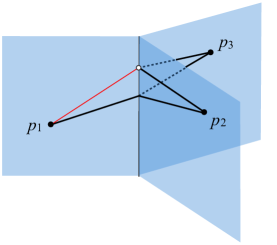
Figure 5: The shortest paths between $p_{1},p_{2},p_{3}$ (shown in black) do not determine the convex hull because the thin red line is on the boundary of the convex hull but not on any of the shortest paths.

Our first example, shown in Figure 5, has three cells sharing an edge. Set $P$ contains one point in each cell. The three shortest paths between pairs of points in $P$ do not determine the convex hull. This shows that property 1 fails.

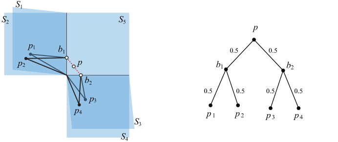
Figure 6: (left) A 2D CAT(0) space consisting of 5 quadrants. Quadrants $S_{1},S_{2},S_{5}$ share a vertical edge, and quadrants $S_{3},S_{4},S_{5}$ share a horizontal edge. Point $p_{i},i=1,2,3,4$, lies in quadrant $S_{i}$. The convex hull of $p_{1},p_{2},p_{3},p_{4}$ contains points—in particular $p$ and the dashed red line—in a quadrant, $S_{5}$, that is not entered by any shortest path between points in $P$ (shown as black lines). Note that 4 of the 6 shortest path between points of $P$ go through the origin. (right) The tree representation of point $p$ in terms of $P$.

Furthermore, the example in Figure 6 shows that even in a single-vertex 2D CAT(0) rectangular complex, the convex hull of a set of points $P$ can contain a point in a quadrant that is not entered by any shortest path between points of $P$. This example also shows that Carathéodory’s property may fail, since point $p$ is in the convex hull of the four points $p_{1},p_{2},p_{3},p_{4}$ but not in the convex hull of any three of the points.

The example in Figure 7 shows that the convex hull of three points in a 3D CAT(0) complex may contain a 3D ball, and thus property 2 fails. Lin et al. [43] give a more complicated family of examples in which the top-dimensional cells have dimension $2d$, and there exist 3 points in the space such that their convex hull contains a $d$-dimensional simplex.

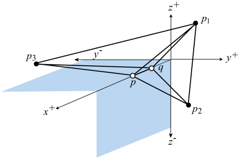
Figure 7: The convex hull of the three points $p_{1},p_{2},p_{3}$ in this 3D CAT(0) complex contains a 3D ball. The complex consists of exactly 3 octants, $x^{+}y^{+}z^{+}$, $x^{+}y^{+}z^{-}$, and $x^{+}y^{-}z^{+}$, and is missing the bottom left octant $x^{+}y^{-}z^{-}$. Point $p_{1}$ lies in the $x^{+}y^{+}z^{+}$ octant, $p_{2}$ in the $x^{+}y^{+}z^{-}$ octant, and $p_{3}$ in the $x^{+}y^{-}z^{+}$ octant. Point $p$ is where the shortest path from $p_{2}$ to $p_{3}$ intersects the $x^{+}$ axis, and point $q$ is where the triangle $p_{1}p_{2}p_{3}$ is pierced by the $x^{+}$ axis. The convex hull of $P$ consists of the union of two simplices $p_{1}p_{3}pq$ and $p_{1}p_{2}pq$.

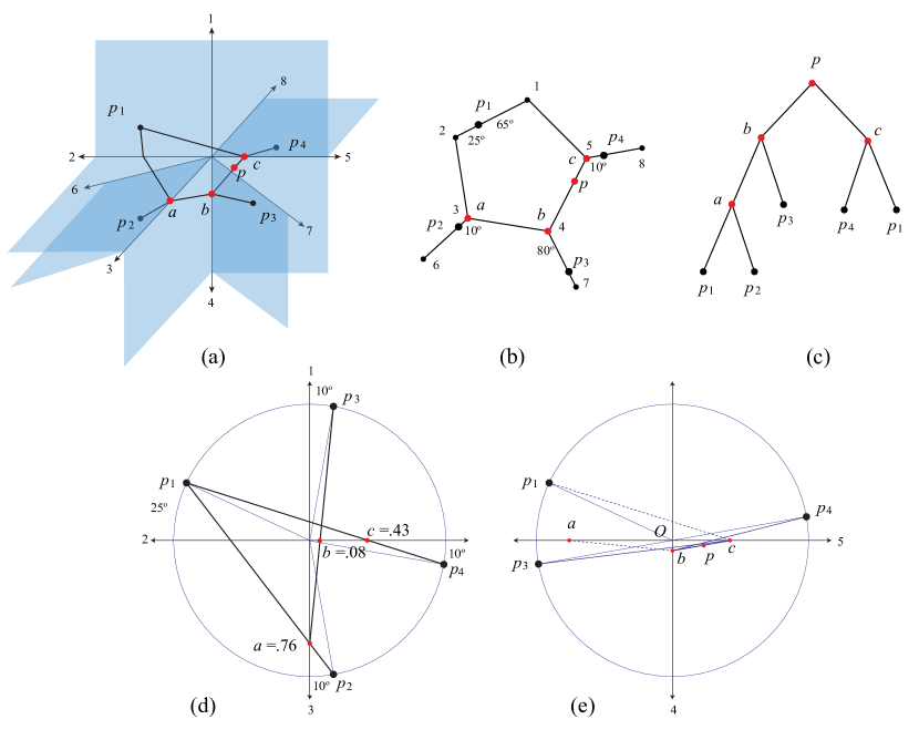
Figure 8: An example of a 2D CAT(0) complex where point $p$ in CH$(\{p_{1},p_{2},p_{3},p_{4}\})$ cannot be represented as a binary tree with distinct leaves. Points $p_{1},p_{2},p_{3},p_{4}$ are all distance 1 from the origin, with angles as specified in the link graph. (a) the complex $\cal K$ (not to scale); (b) the link graph $G$; (c) a binary tree representing $p$ with leaf $p_{1}$ repeated; (d) construction of points $a,c$ and $b$; (e) $p$ does not lie in either the shortest path from $b$ to a point in $Op_{4}$ or the shortest path from $c$ to a point in $Op_{3}$.

Property 3 must be expressed more carefully for CAT(0) complexes because it is not clear what a convex combination of a set of points means except when the set has two points. If $p$ and $q$ are two points in a CAT(0) complex, then the points along the shortest path from $p$ to $q$ can be parameterized as $(1-t)p+tq$ for $t\in[0,1]$. Based on the definition of the convex hull, any point in the convex hull of a set of points $P$ can be represented as a rooted binary tree with leaves labelled by points in $P$ (with repetition allowed) and with the two child edges of each internal node $v$ labelled by two numbers $(1-t_{v})$ and $t_{v}$ for $t_{v}\in[0,1]$, meaning that the point associated with $v$ is this combination of the points represented by the child nodes. For example, see Figure 6.

One might hope that every point in the convex hull can be represented by a binary tree whose leaves are labelled by distinct elements of $P$. If this were true then we could verify that a point is in the convex hull of $m$ points by giving a binary tree with at most $m$ leaves, and the problem of deciding membership in the convex hull would lie in NP, at least for the case of cube complexes, where the sizes of the weights attached to the binary tree are polynomially bounded. However, this hope is dashed by the example in Figure 7. Furthermore, the property may even fail for a 2D CAT(0) complex as we prove below for the example in Figure 8:

Lemma 4.

For the 2D CAT(0) complex shown in Figure 8, the point $p$ cannot be represented by a binary tree with distinct leaves from $\{p_{1},p_{2},p_{3},p_{4}\}$.

Proof.

Point $p$ can be generated by a binary tree with two leaves labelled $p_{1}$, as shown in Figure 8(c). This tree has internal nodes corresponding to points $a,b$ and $c$. The gist of our argument is to show that $p$ cannot be generated without points $b$ and $c$, and each of those requires $p_{1}$ to generate it.

The first part of the argument involves the link graph $G$ shown in Figure 8(b), and the second part involves the actual coordinates (the distance from $O$) of the intermediate points. As shown in Figure 8(d), starting from quadrant $\{1,2\}$ in the upper left, we can compute $a=.76$ and $c=.42$, and from these (unfolding further quadrants on top of each other) $b=.08$. Figure 8(e) shows quadrant $\{4,5\}$ containing $b,c,p$ in the lower right together with neighbouring quadrants. The property we observe from the figure (and could calculate numerically) is that $p$ lies below segment $bp_{4}$ and below segment $cp_{3}$. With these facts in hand, we now give the details of the proof.

Suppose $p$ is represented by a binary tree $T$ with distinct leaves from $\{p_{1},p_{2},p_{3},p_{4}\}$. Let $q_{1}$ and $q_{2}$ be the points of the complex corresponding to the children of the root of $T$. Thus $p$ lies on the shortest path from $q_{1}$ to $q_{2}$. Point $p$ corresponds to a point $\lambda(p)$ that lies in edge $(4,5)$ of the link graph $G$. By Proposition 3, the shortest path between $\lambda(q_{1})$ and $\lambda(q_{2})$ must have length less than $180^{\circ}$, so one of them, say $\lambda(q_{1})$, must lie in edge $(5,1)$ or $(5,8)$ of $G$, and the other, say $\lambda(q_{2})$, must lie in edge $(4,3)$ or $(4,7)$. Furthermore, without loss of generality, the subtree rooted at $q_{1}$ must include the leaf $p_{4}$ and the subtree rooted at $q_{2}$ must include the leaf $p_{3}$, because without those points we cannot generate anything in the appropriate edges of $G$.

Point $p_{1}$ may be a leaf of the subtree rooted at $q_{1}$ (case 1) or the subtree rooted at $q_{2}$ (case 2), but not both.

In case 1, the subtree rooted at $q_{2}$ has leaf $p_{3}$ and possibly $p_{2}$. In $G$, the shortest path between $p_{2}$ and $p_{3}$ has length $180^{\circ}$ so, by Proposition 3, the geodesic between $p_{2}$ and $p_{3}$ in the complex is a “cone path” that goes through the origin. Thus $q_{2}$ must be a point in the segment $Op_{3}$. The subtree rooted at $q_{1}$ has leaves $p_{4},p_{1}$ and possibly $p_{2}$. As shown in Figure 8(e), the extreme points we can generate are $p_{4}$, $c$, and $O$. However, for any point $q_{1}$ in this triangle, and any point $q_{2}$ in $Op_{3}$, the shortest path between $q_{1}$ and $q_{2}$ does not go through $p$. This rules out case 1.

In case 2, the subtree rooted at $q_{1}$ has leaf $p_{4}$ and possibly $p_{2}$. Since the path between these points is a cone path, $q_{1}$ must be a point in the segment $Op_{4}$. The subtree rooted at $q_{2}$ has leaves $p_{3},p_{1}$, and possibly $p_{2}$. As shown in Figure 8(e), the extreme points we can generate are $p_{3}$, $b$, and $O$. However, for any point $q_{2}$ in this triangle, and any point $q_{1}$ in $Op_{4}$, the shortest path between $q_{1}$ and $q_{2}$ does not go through $p$. This rules out case 2.

Therefore, $p$ cannot be represented by a binary tree with distinct leaves from $\{p_{1},p_{2},p_{3},p_{4}\}$. ∎

4.3 Convex Hull Algorithm for a Single-Vertex 2D CAT(0) Complex

In this section we prove Theorem 2 by reducing the convex hull problem for a single-vertex 2D CAT(0) complex $\cal K$ to linear programming via a polynomial-time reduction in the real RAM model of computation. Recall that $P$ is the finite set of points whose convex hull we wish to find, and $O$ is the single vertex of the complex.

We will find the convex hull as a union of convex polygons, one for each cell of $\cal K$. To justify this, observe that the intersection of ${\rm CH}(P)$ with cell $C$ of $\cal K$ is a convex polygon (which may be open or closed on parts of its boundary), and ${\rm CH}(P)$ is the union of these polygons.

The recursive definition of the convex hull of $P$ involves taking all pairs of points $p,q$ in the set and adding all points along the unique geodesic from $p$ to $q$. We consider using a restricted set of points, namely, those that lie in $P$ and on the edges of $\cal K$.

Define $S_{0}$ to be the set $P$ together with point $O$ if it is in the convex hull of $P$. For $i=1,2,\ldots$ we recursively define a finite set of points $S_{i}$, called the $i^{\rm th}$ skeleton, as follows. Initialize a set $T_{i}$ to be $S_{i-1}$. For each pair of points $p,q$ in $S_{i-1}$, take the shortest path, $\sigma$, in $\cal K$ from $p$ to $q$. Add to $T_{i}$ all the intersection points of $\sigma$ with edges of the complex. Observe that $T_{i}$ is a finite set. For any edge $e$ of the complex, if $T_{i}$ contains more than 2 points of $e$, then discard all but the two extreme points, $S_{i}^{\max}(e)$ and $S_{i}^{\min}(e)$. In case $O$ is in the convex hull, then $S_{i}^{\min}(e)=O$. Now define $S_{i}$ to be $T_{i}$.

We can augment each skeleton $S_{i}$ to a larger subset of ${\rm CH}(P)$ as follows. For each cell $C$ of the complex, let $S_{i}(C)$ be the points of $S_{i}$ that lie in the closed cell $C$. Thus $S_{i}(C)$ consists of: the points of $P$ that lie in $C$; point $O$ if it lies in ${\rm CH}(P)$; and between 0 and 4 points that lie on the two boundary rays of $C$. Define $H_{i}(C)$ to be the Euclidean convex hull of $S_{i}(C)$ in $C$ and define $H_{i}=\bigcup\{H_{i}(C):C$ a cell of ${\cal K}\}$. Observe that $H_{i}\subseteq{\rm CH}(P)$.

We justify the restriction to skeletons by showing that each $H_{i}$ contains all shortest paths between points of $H_{i-1}$:

Theorem 5.

Let $p$ and $q$ be points of $H_{i-1}$ and let $\sigma$ be the shortest path in $\cal K$ from $p$ to $q$. Then $\sigma\subseteq H_{i}$.

Proof.

Suppose that $p\in H_{i-1}(C_{p})$ and $q\in H_{i-1}(C_{q})$ for some cells $C_{p}$ and $C_{q}$. If $p$ or $q$ lies on a cell boundary, and thus could be assigned to more than one cell, choose the cell assignments to minimize the number of cells traversed by the geodesic between $p$ and $q$. In particular, if $p$ and $q$ lie in the same edge, or if one of them is at $O$, then assign both points to the same cell. If $C_{p}=C_{q}$ then $\sigma\subseteq H_{i-1}(C_{p})$ since $H_{i-1}(C_{p})$ is a convex set. In this case we are done because $H_{i-1}(C_{p})\subseteq H_{i}(C_{p})$.

If $\sigma$ goes through $O$, then $\sigma$ consists of two subpaths from $p$ to $O$ and from $O$ to $q$ and these subpaths lie in $H_{i-1}(C_{p})$ and $H_{i-1}(C_{q})$ respectively, so we are also done in this case.

Otherwise, suppose that $\sigma$ crosses the sequence of cells $C_{p}=C_{0},C_{1},\ldots,C_{t}=C_{q}$. We can unfold these cells in the plane so that $\sigma$ becomes a straight line. See Figure 9. For $j=1,\ldots,t$ let $e_{j}$ be the edge (or ray) of $\cal K$ between $C_{j-1}$ and $C_{j}$, and let $p_{j}$ be the point where $\sigma$ crosses $e_{j}$. Let $p_{0}=p$ and $p_{t+1}=q$. It suffices to show that $p_{j}\in H_{i}$ for all $j$, since this implies that the subpath of $\sigma$ from $p_{j-1}$ to $p_{j}$ lies in $H_{i}(C_{j-1})$.

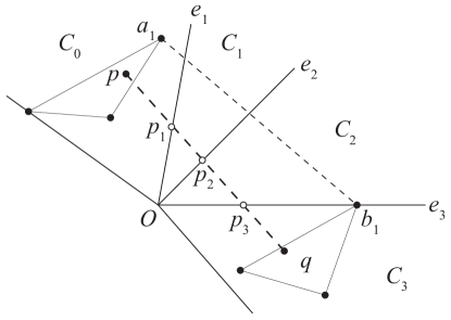
Figure 9: Illustration for the proof of Theorem 5.

Because $p$ lies in $H_{i-1}(C_{p})$, which is the Euclidean convex hull of $S_{i-1}(C_{p})$, there must be points $a_{1},a_{2},a_{3}$ in $S_{i-1}(C_{p})$ with $p$ inside the triangle $a_{1}a_{2}a_{3}$. We note that the triangle may degenerate to a line segment (or even to a point, in case $p\in S_{i-1}(C_{p})$). Similarly, there must be points $b_{1},b_{2},b_{3}$ in $S_{i-1}(C_{q})$ with $q$ inside the (possibly degenerate) triangle $b_{1}b_{2}b_{3}$.

In the planar unfolding of cells $C_{0},C_{1},\ldots,C_{t}$, extend $\sigma$ to a straight line $L$. Note that $L$ does not go through $O$ otherwise $p$ and $q$ would lie in the same cell. Let the “near side” of $L$ be the (closed) side containing $O$, and the “far side” be the other (closed) side. At least one of the $a_{k}$’s, say $a_{1}$, must be on the far side of $L$. Similarly, at least one of the $b_{k}$’s, say $b_{1}$, must be on the far side of $L$. Then the shortest path from $a_{1}$ to $b_{1}$ in $\cal K$ unfolds to the straight line segment $a_{1}b_{1}$. (To justify this, note that the angle $a_{1}Ob_{1}$ is less than $\pi$ because $a_{1}$ and $b_{1}$ are on the far side of $L$.) The line segment $a_{1}b_{1}$ crosses each edge $e_{j}$ on the far side of $L$. By the definition of $S_{i}$ each such crossing point, or a point even farther along $e_{j}$, becomes a point of $S_{i}$.

We can make the same argument about the near side of $L$. Suppose points $a_{2}$ and $b_{2}$ are on the near side of $L$. The shortest path from $a_{2}$ to $b_{2}$ either goes through $O$, or becomes a straight line segment in the unfolding. In either case, every edge $e_{j}$ contains a point of $S_{i}$ that is on the near side of $L$.

Because point $p_{j}$ is between two points of $S_{i}$ on $e_{j}$, thus $p_{j}\in H_{i}$. ∎

Corollary 6.

${\rm CH}(P)=\bigcup_{i}H_{i}$.

Alternatively, we can express ${\rm CH}(P)$ in terms of a set $S$ that is the limit of the $S_{i}$’s. For each edge $e$ of $\cal K$, the sequence of points $S_{i}^{\min}(e),i=0,1,\ldots$ is decreasing and bounded below by $O$. The set $S_{i}^{\max}(e),i=0,1,\ldots$ is increasing and bounded above. (Note that no point of ${\rm CH}(P)$ will be further from $O$ than the furthest point of $P$.) Thus the limit points $S^{\min}(e)$ and $S^{\max}(e)$ exist. Define $S$ to be the union of $P$ and the set of limit points on all edges $e$.

Similar to the definition of $H_{i}$ from $S_{i}$, we define $H(C)$ to be the Euclidean convex hull of $S\cap C$ for each cell $C$, and then define $H$ to be $\bigcup\{H(C):C$ a cell of ${\cal K}\}$. Certainly ${\rm CH}(P)\subseteq H$. Whether they are equal is the same as the question of whether ${\rm CH}(P)$ is closed, as the following proposition shows.

Proposition 7.

$H$ is the closure of ${\rm CH}(P)$.

Proof.

$H$ is a closed set containing ${\rm CH}(P)$, so $H$ contains the closure of ${\rm CH}(P)$. In the other direction, the closure of ${\rm CH}(P)$ contains $S$ and therefore contains $H$. ∎

Our approach to proving Theorem 2 is to compute $H$, the closure of ${\rm CH}(P)$, by capturing the limit skeleton $S$ via linear programming.

A more obvious approach to computing ${\rm CH}(P)$ would be to compute the sequence of $S_{i}$’s. Such a procedure is finite if and only if ${\rm CH}(P)$ is closed:

Proposition 8.

${\rm CH}(P)$ is closed if and only if the sequence $S_{0},S_{1},\ldots$ is finite (i.e., $S_{k}=S_{k+1}$ for some $k$).

Proof.

If ${\rm CH}(P)$ is closed then for each edge $e$ of $\cal K$, the extreme points of ${\rm CH}(P)$ on $e$ must enter $S_{i}$ for some $i$. The set of such extreme points is finite (there are at most two per edge), so all of them are contained in $S_{k}$ for some $k$. Then $S_{k}=S_{k+1}$.

In the other direction, if $S_{k}=S_{k+1}$ then $H_{k}=H_{k+1}$. Also $S=S_{k}$ and $H=H_{k}$. By Corollary 6, ${\rm CH}(P)=\bigcup_{i}H_{i}$. Then $\bigcup_{i}H_{i}=\bigcup_{i}^{k}H_{i}=H_{k}=H$, so ${\rm CH}(P)=H$. By Proposition 7, $H$ is the closure of ${\rm CH}(P)$ so this implies that ${\rm CH}(P)$ is closed. ∎

We conjecture that ${\rm CH}(P)$ is closed, and thus that we can compute ${\rm CH}(P)$ by computing each $S_{i}$ until no further changes occur. This would be efficient if there were a good bound on the length of the sequence. We conjecture that there is such a bound:

Conjecture 1.

$S_{k}=S_{k+1}$ for some $k$ that is polynomially bounded in $n$ and $m$.

4.3.1 Combinatorics of the Convex Hull

For our linear programming approach we need to know whether $O$ is in the convex hull, and we need to identify the edges of $\cal K$ that contain points of the convex hull other than $O$. We give algorithms for these using the link graph $G=G_{O}$. Let $V$ be the set of vertices of $G$; recall that these correspond to the edges of $\cal K$.

We begin by showing that we can compute the projection of the convex hull of $P$ on the link graph. We introduce some notation to make this formal. For any point $p\in{\cal K}-\{O\}$, denote the corresponding point in the link graph by $\lambda(p)$. We extend this notation to subsets of $\cal K$—for a set $S\subseteq{\cal K}$, define $\lambda(S)$ as $\{\lambda(p):p\in S-\{O\}\}$. In particular, $\lambda({\rm CH}(P))$ denotes the projection of the convex hull of $P$ on the link graph.

We introduce the link convex hull, ${\rm LCH}(P)$, a subset of $G$ defined recursively as follows: (1) $\lambda(P)$ is contained in ${\rm LCH}(P)$; (2) For any two points $a,b$ in ${\rm LCH}(P)\cap(\lambda(P)\cup V)$, if the shortest path $\sigma_{G}(a,b)$ has length less than $\pi$ then all the points of $\sigma_{G}(a,b)$ are contained in ${\rm LCH}(P)$. In other words, we take the closure of $\lambda(P)$ in the link graph under the operation of taking shortest paths between pairs of points, but only when the points are vertices or correspond to points in $P$, and only when the paths have length less than $\pi$. Note that ${\rm LCH}(P)$ is not a subgraph of $G$ because in general it includes portions of edges.

We will show that $\lambda({\rm CH}(P))={\rm LCH}(P)$, and that ${\rm LCH}(P)$ can be computed in a straight-forward way. From ${\rm LCH}(P)$ we can readily identify the edges of $\cal K$ that contain points of the convex hull other than $O$—these correspond to vertices of the link graph in ${\rm LCH}(P)$. We will also show how to use ${\rm LCH}(P)$ to decide if $O$ is in ${\rm CH}(P)$.

Lemma 9.

$\lambda({\rm CH}(P))={\rm LCH}(P)$.

Proof.

We first prove ${\rm LCH}(P)\subseteq\lambda({\rm CH}(P))$ by structural induction based on the recursive definition of ${\rm LCH}(P)$. As the base case we have $\lambda(P)\subseteq\lambda({\rm CH}(P))$. For the recursive step let $a,b$ be two points in ${\rm LCH}(P)\cap(\lambda(P)\cup V)$ such that $|\sigma_{G}(a,b)|<\pi$. Assume by induction that $a,b\in\lambda({\rm CH}(P))$, in particular, that $a=\lambda(a^{\prime})$ and $b=\lambda(b^{\prime})$ with $a^{\prime},b^{\prime}\in{\rm CH}(P)$. Then $\sigma(a^{\prime},b^{\prime})\subseteq{\rm CH}(P)$. Since $|\sigma_{G}(a,b)|<\pi$, Proposition 3 implies that $\lambda(\sigma(a^{\prime},b^{\prime}))=\sigma_{G}(a,b)$. Therefore $\sigma_{G}(a,b)\subseteq\lambda({\rm CH}(P))$.

Next we prove $\lambda({\rm CH}(P))\subseteq{\rm LCH}(P)$ by structural induction based on the recursive definition of ${\rm CH}(P)$. As the base case we have $\lambda(P)\subseteq{\rm LCH}(P)$. For the recursive step, let $a$ and $b$ be two points in ${\rm CH}(P)$. Assume by induction that $\lambda(a),\lambda(b)\in{\rm LCH}(P)$. We must show that $\lambda(\sigma(a,b))\subseteq{\rm LCH}(P)$. If $|\sigma_{G}(\lambda(a),\lambda(b))|\geq\pi$ then by Proposition 3 the shortest path from $a$ to $b$ in $\cal K$ goes through $O$. In this case $\lambda(\sigma(a,b))$ consists only of points $\lambda(a)$ and $\lambda(b)$, which are in ${\rm LCH}(P)$ by assumption. Thus we can restrict attention to the case where $|\sigma_{G}(\lambda(a),\lambda(b))|<\pi$. By Proposition 3 this implies that $\lambda(\sigma(a,b))=\sigma_{G}(\lambda(a),\lambda(b))$. Thus we must show that $\sigma_{G}(\lambda(a),\lambda(b))\subseteq{\rm LCH}(P)$, i.e. that every point in $\sigma_{G}(\lambda(a),\lambda(b))$ lies in ${\rm LCH}(P)$.

If $\lambda(a)$ and $\lambda(b)$ lie in $\lambda(P)\cup V$, this is immediate, but otherwise we must examine why $\lambda(a)$ and $\lambda(b)$ are in ${\rm LCH}(P)$. If $\lambda(a)\in\lambda(P)\cup V$, let $A=A^{\prime}=\lambda(a)$. Otherwise, suppose that $\lambda(a)$ is an internal point of edge $e_{a}$ of $G$. By the definition of ${\rm LCH}(P)$, there must be points $A$ and $A^{\prime}$ in ${\rm LCH}(P)\cap(\lambda(P)\cup V)$ such that $\sigma_{G}(A,A^{\prime})$ has length less than $\pi$ and includes $\lambda(a)$. Choose such $A$ and $A^{\prime}$ so that $|\sigma_{G}(A,A^{\prime})|$ is minimum. Then each of $A$ and $A^{\prime}$ is either an endpoint of $e_{a}$ or a point of $\lambda(P)$ internal to $e_{a}$.

We now do the same for $b$. If $\lambda(b)\in\lambda(P)\cup V$, let $B=B^{\prime}=\lambda(b)$. Otherwise, suppose that $\lambda(b)$ is an internal point of edge $e_{b}$ of $G$. By the definition of ${\rm LCH}(P)$, there must be points $B$ and $B^{\prime}$ in ${\rm LCH}(P)\cap(\lambda(P)\cup V)$ such that $\sigma_{G}(B,B^{\prime})$ has length less than $\pi$ and includes $\lambda(b)$. Choose such $B$ and $B^{\prime}$ so that $|\sigma_{G}(B,B^{\prime})|$ is minimum. Then each of $B$ and $B^{\prime}$ is either an endpoint of $e_{b}$ or a point of $\lambda(P)$ internal to $e_{b}$.

If $e_{a}\neq e_{b}$ then there must be a point of $\{A,A^{\prime}\}$, say $A$, in $\sigma_{G}(\lambda(a),\lambda(b))$, and there must be a point of $\{B,B^{\prime}\}$, say $B$, also in $\sigma_{G}(\lambda(a),\lambda(b))$. See Figure 10. Then $\sigma_{G}(A,B)$ has length less than $\pi$ since it is a subpath of $\sigma_{G}(\lambda(a),\lambda(b))$. Now we have $\sigma_{G}(\lambda(a),\lambda(b))\subseteq\sigma_{G}(A,A^{\prime})\cup\sigma_{G}(A,B)\cup\sigma_{G}(B,B^{\prime})$. All three of these paths have length less than $\pi$ and have endpoints in ${\rm LCH}(P)\cap(\lambda(P)\cup V)$. Thus the paths lie in ${\rm LCH}(P)$, so $\sigma_{G}(\lambda(a),\lambda(b))\subseteq{\rm LCH}(P)$. If $e_{a}=e_{b}$ we may still have points $A$ and $B$ in $\sigma_{G}(\lambda(a),\lambda(b))$—in which case the previous argument applies. And otherwise $\sigma_{G}(\lambda(a),\lambda(b))\subseteq\sigma_{G}(A,A^{\prime})$, and this still gives $\sigma_{G}(\lambda(a),\lambda(b))\subseteq{\rm LCH}(P)$. ∎

Figure 10: Illustration for the proof of Lemma 9. $\sigma_{G}(\lambda(a),\lambda(b))\subseteq\sigma_{G}(A^{\prime},A)\cup\sigma_{G}(B,B^{\prime})\cup\sigma_{G}(A,B)$. Top: $e_{a}\neq e_{b}$. Bottom: two cases where $e_{a}=e_{b}$.

Computing ${\rm LCH}(P)$. We can find the points of ${\rm LCH}(P)$ in $\lambda(P)\cup V$ as follows. We build up a set $A\subseteq\lambda(P)\cup V$. Initially $A$ will just be the input set of points $\lambda(P)$, and at the end of the algorithm, $A$ will be the required set. We will also keep a subset $F$ of $A$ that represents the “frontier” that we still need to explore from. Initially $F=A=\lambda(P)$.

The general step is to remove one element $v$ from $F$. We then explore the part of the link graph within distance $<\pi$ from $v$. This can be done by a depth-first search in $O(n+m)$ time. A search tree to distance $\pi$ will find no cycles, and will therefore find shortest paths from $v$. We remove the part of the depth-first tree that is beyond the deepest point of $A$ on each branch. Then for every vertex $w$ of the link graph that is in the depth-first search tree, we check if $w$ is already in $A$—if not then we add $w$ to $A$ and to $F$.

The size of $A$ is bounded by $n+m$ where $n$ is the number of cells in $\cal K$ and $m$ is the size of $P$. Note that the amount of work we do for one element of $F$ is $O(n+m)$. Thus the algorithm runs in time $O((n+m)^{2})$.

Testing if $O$ is in the convex hull. If $O\in P$ we are done, so we must just deal with the case when $O\not\in P$.

Lemma 10.

Suppose that $O\not\in P$. Then $O$ is in ${\rm CH}(P)$ if and only if there are two points in ${\rm LCH}(P)$ such that the distance between them is at least $\pi$.

Proof.

By definition, $O$ is in ${\rm CH}(P)$ if and only if there are two points $a$ and $b$ in ${\rm CH}(P)-O$ such that the shortest path between them goes through $O$. By Proposition 3 this is equivalent to there being two points in $\lambda({\rm CH}(P))$ whose distance in $G$ is at least $\pi$. By Lemma 9 $\lambda({\rm CH}(P))={\rm LCH}(P)$ which gives the desired result. ∎

We can test if there are two points of $P$ whose shortest path goes through $O$. The remaining case is solved by the following lemma:

Lemma 11.

Suppose that $O\not\in P$ and no shortest path between two points of $P$ goes through $O$. Then $O\in{\rm CH}(P)$ if and only if ${\rm LCH}(P)$ contains a cycle.

Proof.

Suppose ${\rm LCH}(P)$ contains a cycle. Because the space is CAT(0), the cycle has length at least $2\pi$, so it must contain two points $a,b$ whose minimum distance in the cycle is $\pi$. We claim that the shortest path from $a$ to $b$ in the link graph has length $\pi$—if there were a shorter path then, together with the path in the cycle of length $\pi$ we would get a second cycle of length $<2\pi$. Thus the shortest path from $a$ to $b$ has length $\pi$ and by Lemma 10, $O$ is in ${\rm CH}(P)$.

For the other direction, suppose ${\rm LCH}(P)$ does not contain a cycle. ${\rm LCH}(P)$ is connected, so it must be a tree. We claim that the leaves of the tree are points of $\lambda(P)$: If $d$ is a point of ${\rm LCH}(P)$ that is not in $\lambda(P)$, then $d$ was placed in ${\rm LCH}(P)$ because it is the internal point of some shortest path between points in ${\rm LCH}(P)$, so $d$ has degree at least 2 in ${\rm LCH}(P)$, so it is not a leaf.

Let $a$ and $b$ be points of ${\rm LCH}(P)$. The path between $a$ and $b$ in the tree ${\rm LCH}(P)$ can be extended to a path between leaves of ${\rm LCH}(P)$, and, since the leaves are in $\lambda(P)$, this path has length less than $\pi$. Thus by Lemma 10, $O$ is not in the convex hull. ∎

4.3.2 Finding the Convex Hull via Linear Programming

In this section we give a polynomial-time algorithm to construct a linear program to find the convex hull of a finite point set $P$ in a 2D CAT(0) complex $\cal K$ with a single vertex $O$.

Recall the skeletons, $S_{i}$, from Section 4.3, which give an iterative way of computing the extreme points of the convex hull along each edge of the complex. As $i$ increases, the extreme points expand outwards. The idea of our linear program is to have two variables for each edge $e$ that represent the two extreme points of $S_{i}$ on $e$. The linear constraints will express the closure-under-shortest-paths property that was used to construct $S_{i+1}$ from $S_{i}$. Thus feasible solutions to the linear program will represent limit points $S$ of the $S_{i}$’s. From these points, we can compute ${\rm CH}(P)$, as justified by Corollary 6. Furthermore, the computation of ${\rm CH}(P)$ from the set $S$ is efficient since it simply involves computing the Euclidean convex hull inside each cell $C$, and Euclidean (planar) convex hulls can be computed in polynomial time [16]. We now fill in the details of this plan.

Our algorithm and our notation will be simpler if the points of $P$ all lie on edges of the complex. In particular, the convex hull inside a cell $C$, if non-empty, will be a triangle or quadrilateral (depending on whether $O$ is in the convex hull) since no points of $P$ will be internal to $C$. We can achieve this by constructing a new edge $e_{p}$ from $O$ through each point $p\in P$ (except the point $O$). Each such edge divides a cell in two. Point $p$ is then represented in local coordinates by the distance along edge $e_{p}$ from $O$ to point $p$. We will use $p$ to refer both to the point and to its local coordinate, i.e., its distance from $O$ (in the same way that we refer to a point on the real line as a number).

Let $B$ be the set of edges of the complex that contain points other than $O$ inside the convex hull. These correspond to points of ${\rm LCH}(P)$ in $V$ and can be found as described in the previous section.

For clarity of presentation we will separate into two cases depending on whether the origin is inside the convex hull.

When the origin $O$ is inside the convex hull. For each $\ell\in B$ our linear program will have a variable $x_{\ell}\in{\mathbb{R}}$ representing the distance from $O$ to the point on $\ell$ that is on the boundary of the convex hull. Then $x_{\ell}>0$. Note that, like $p$, $x_{\ell}$ refers both to a distance and a point.

Our inequalities are of two types. First, for any point $p\in P$ lying on an edge $\ell\in B$ we include the inequality:

$$x_{\ell}\geq p$$ (1)

Inequalities of the second type will be determined by pairs of elements from the set $B$. For any two edges $e$ and $f$ of $B$, such that the angle between $e$ and $f$ is $<\pi$, consider the shortest path $\sigma$ between the corresponding points $x_{e}$ and $x_{f}$. We will add a constraint for each edge $\ell$ of $B$ crossed by $\sigma$, expressing the fact that the convex hull includes the point where $\sigma$ crosses $\ell$. The constraint has the form $x_{\ell}\geq t$ where $t$ is the distance from $O$ to the point where $\sigma$ crosses $\ell$. We will use $t$ to refer to both the distance and to the point. We can express $t$ in terms of known quantities. The set-up is illustrated in Figure 11. Note that there may be several polyhedral cells separating $e$ and $f$, but we can unfold them in the plane to form a triangle.

Figure 11: Expressing the intersection point $t$ in terms of known quantities.

Let $\gamma_{1}$ be the angle between $e$ and $\ell$, and let $\gamma_{2}$ be the angle between $\ell$ and $f$. Then we have:

Claim 1.

$$t=\frac{x_{e}x_{f}\sin(\gamma_{1}+\gamma_{2})}{x_{e}\sin\gamma_{1}+x_{f}\sin\gamma_{2}}$$

Proof.

Let $A$ denote the area of a triangle. Observe that $A(O,x_{e},t)+A(O,t,x_{f})=A(O,x_{e},x_{f})$. Applying the sine law for area of a triangle, we obtain

$$\frac{1}{2}x_{e}t\sin\gamma_{1}+\frac{1}{2}tx_{f}\sin\gamma_{2}=\frac{1}{2}x_{e}x_{f}\sin(\gamma_{1}+\gamma_{2}).$$

Rearranging gives the required formula for $t$. ∎

Using the above claim, the constraint $x_{\ell}\geq t$ becomes

$$x_{\ell}\geq\frac{x_{e}x_{f}\sin(\gamma_{1}+\gamma_{2})}{x_{e}\sin\gamma_{1}+x_{f}\sin\gamma_{2}}$$

This is not a linear inequality, but substituting $y_{\ell}={1\over x_{\ell}}$ yields

$$y_{\ell}\leq y_{f}\frac{\sin\gamma_{1}}{\sin(\gamma_{1}+\gamma_{2})}+y_{e}\frac{\sin\gamma_{2}}{\sin(\gamma_{1}+\gamma_{2})}$$ (2)

Since the $\gamma_{i}$’s are constant, this is a linear inequality.

The inequalities (1) for point $p\in P$ on edge $\ell$ become

$$y_{\ell}\leq\frac{1}{p}$$ (3)

Lemma 12.

Maximizing $\sum y_{\ell}$ subject to the inequalities (2), (3) and $y_{\ell}\geq 0$ gives the closure of the convex hull of $P$, i.e., gives the points $x_{\ell}=\frac{1}{y_{\ell}}$ where the closure of the convex hull intersects each edge $\ell\in B$.

Proof.

Recall the definition of the limit set $S$ from the beginning of Section 4.3. Note that the points $S$ provide a feasible solution to the linear system, because they satisfy the constraints $x_{\ell}\geq p$ and $x_{\ell}\geq t$ which we used to construct our inequalities. Denote this solution by $y^{\rm CH}_{\ell},\ell\in B$.

Next, note that any other solution $y^{\prime}_{\ell},\ell\in B$, has $y^{\prime}_{\ell}\leq y^{\rm CH}_{\ell}$ for all $\ell\in B$, i.e. $x^{\prime}_{\ell}\geq x^{\rm CH}_{\ell}$—in other words, any other solution includes $S$. This is because the points of $P$ are included, and the inequalities of our linear system enforce closure under shortest paths. Therefore, the solution that maximizes $\sum y_{\ell}$ gives the points $S$, and thus the set $H$, which is the closure of ${\rm CH}(P)$. ∎

This completes the reduction to linear programming when $O$ is in the convex hull.

When the origin $O$ is not inside the convex hull. In this case, by Lemma 11, the subgraph of the link graph corresponding to the convex hull is a tree, and it seems even more plausible that an efficient iterative approach can be used to find the convex hull. However, we leave this as an open question, and give a linear programming approach like the one above.

For each $\ell\in B$ we will make two variables, $x_{\ell}^{\rm min}$ and $x_{\ell}^{\rm max}$ in ${\mathbb{R}}$ representing the minimum and maximum points on $\ell$ that are on the boundary of the convex hull. To find the closure of the convex hull, it suffices to find the values of these variables.

We want to ensure that $x_{\ell}^{\rm max}$ is larger than any point of $P$ and any point at which a geodesic between $x_{e}^{\rm max}$ and $x_{f}^{\rm max}$, for any $e,f\in B$, crosses edge $\ell$. Similarly, we want to ensure that $x_{\ell}^{\rm min}$ is smaller than any point of $P$ and any point at which a geodesic between $x_{e}^{\rm min}$ and $x_{f}^{\rm min}$, for any $e,f\in B$, crosses edge $\ell$. Using the same notation and set-up as above with edges $e$ and $f$, and using the inverse variables $y_{\ell}^{\rm min}={1\over x_{\ell}^{\rm min}}$ and $y_{\ell}^{\rm max}={1\over x_{\ell}^{\rm max}}$ the inequalities corresponding to (2) are:

$$y^{\rm max}_{\ell}\leq y^{\rm max}_{f}\frac{\sin\gamma_{1}}{\sin(\gamma_{1}+\gamma_{2})}+y^{\rm max}_{e}\frac{\sin\gamma_{2}}{\sin(\gamma_{1}+\gamma_{2})}$$

$$y^{\rm min}_{\ell}\geq y^{\rm min}_{f}\frac{\sin\gamma_{1}}{\sin(\gamma_{1}+\gamma_{2})}+y^{\rm min}_{e}\frac{\sin\gamma_{2}}{\sin(\gamma_{1}+\gamma_{2})}$$

The inequalities corresponding to (3) are:

$$y^{\rm max}_{\ell}\leq\frac{1}{p}\leq y^{\rm min}_{\ell}$$

If we maximize the objective function $\sum(y^{\rm max}_{\ell}-y^{\rm min}_{\ell})$ subject to the above inequalities and $y^{\rm min}_{\ell}\geq y^{\rm max}_{\ell}\geq 0$ then, by a similar argument to the one above, this gives the closure of the convex hull of $P$. Thus we have reduced the problem of finding the convex hull to linear programming.

Running time. We will concentrate on the case where $O$ is in the convex hull—the other case is similar. Recall that $n$ is the number of cells in the complex and $m$ is the number of points in $P$. At the beginning of the algorithm we test if $O$ is in the convex hull, and find the set $B$ of edges of the complex that contain points of the convex hull other than $O$. This takes $O((n+m)^{2})$ time as discussed in the previous section. The set $B$ has size $O(m+n)$ because it includes an edge of the complex through every point of $P$. The linear program has $O(n+m)$ variables. The number of inequalities is $O((n+m)^{3})$ since we consider each pair of elements, $e,f$ from $B$, and add an inequality for each edge of the complex crossed by the shortest path from $e$ to $f$. We can construct the linear program in polynomial time assuming a real RAM model of computation. We need more than arithmetic operations in our real RAM, but what we need depends on exactly how the input is given. The algorithm, as written above, assumes that the input triangles are given in terms of angles. In that case, our real RAM must be able to compute sines of those angles. An alternative is that the input is given to us with each triangle expressed in a local coordinate system. In that case, the sines can be computed from the local coordinates so long as our real RAM includes the square root operation.

The special case of a cube complex

In the special case of a cube complex, it is more natural to give each input point using $x$- and $y$-coordinates relative to the quadrant containing the point. In this case, we claim that all the low-level computations described above can be performed in polynomial time when measuring bit complexity. We will not construct new edges through points of $P$ since that introduces new angles. Our variables are $x_{e}$ for $e$ an edge of the complex, and we add constraints for shortest paths between pairs of points in $P\cup\{x_{e}\}$.

We give a few more details for the computation of $t$ in Figure 11 in this case. Figure 11 shows a path between $x_{e}$ and $x_{f}$ crossing an edge $\ell$ at $t$. In the current setting, $\ell$ will be an edge of $\cal K$, and $x_{e}$ and $x_{f}$ may be variables or input points. If $x_{e}$ and $x_{f}$ correspond to input points, then $t$ is just the point where a line between two known points crosses an axis. Then the right-hand-side of the corresponding constraint (2) is a constant whose bit complexity is polynomially bounded in terms of the input bit complexity. The case when both $x_{e}$ and $x_{f}$ are variables cannot arise because they would be distance $\pi$ apart in the link graph. Thus the only case we must take care of is when $x_{e}$ corresponds to an input point and $x_{f}$ is a variable (or vice versa). The situation is shown in Figure 12, with $x_{e}$ being an input point $p$ with coordinates $(h,v)$ as shown. Then $t=vx_{f}/(x_{f}+h)$, so constraint (2) becomes $y_{\ell}\leq(hy_{f}+1)/v$. Thus the coefficients in our linear constraints are rationals whose bit complexity is polynomially bounded in terms of the input bit complexity. This means that we can use polynomial-time linear programming algorithms [39, 38] to find the value of $x_{e}$ for each edge $e$ of $\cal K$.

Figure 12: Expressing the intersection point $t$ in terms of known quantities in the case of a cube complex.

This completes the proof of Theorem 2.

5 Shortest Paths

In this section we explore the possibilities and limitations of using the shortest path map to solve the single-source shortest path problem in a 2D CAT(0) complex. The input is a 2D CAT(0) complex, $\cal K$, composed of $n$ triangles, and a “source” point $s$ in $\cal K$. We denote the shortest path from $s$ to $t$ by $\sigma(s,t)$. Throughout this section, the cells of $\cal K$ will be called “faces”.

In general, the shortest path map partitions the space into regions in which all points have shortest paths from $s$ that have the same combinatorial type. Specialized to 2D CAT(0) complexes, two shortest paths have the same combinatorial type if they traverse the same sequence of edges, vertices, and faces. A basic approach to the single source shortest path problem is to compute the whole shortest path map from $s$.

We first show that the shortest path map may have exponential size for a general 2D CAT(0) complex. This contrasts with the fact that the shortest path map has size $O(n^{2})$ in the two special cases where the single-source shortest path problem is known to be efficiently solvable: when the complex is a topological 2-manifold with boundary, which we will call a 2-manifold for short [44]; and when the complex is rectangular [22].

We then show that for any 2D CAT(0) complex there is a structure called the “last step shortest path map” that coarsens the shortest path map, has size $O(n)$, and allows us to find the shortest path $\sigma(s,t)$ to a given target point $t$ in time proportional to the number of triangles and edges traversed by the path. Although we do not know how to find the last step shortest path map in polynomial time for general 2D CAT(0) complexes, we can obtain it from the shortest path map.

From this, we obtain efficient algorithms for the single-source shortest path problem in 2D CAT(0) complexes that are 2-manifold or rectangular. Both cases had been previously solved, but the techniques used in the two cases were quite different. Our approach is the same in both cases and opens up the possibility of solving other cases. We need $O(n^{2})$ preprocessing time and space to construct a structure that uses $O(n)$ space and allows us to find the shortest path $\sigma(s,t)$ to a given target point $t$ in time proportional to the number of triangles and edges traversed by the path. This matches the previous time bounds.

5.1 The Shortest Path Map

Typically in a shortest path problem, the difficulty is to decide which of multiple geodesic (or locally shortest) paths to the destination is shortest. This is the case, for example, for shortest paths in a planar polygon with holes, or for shortest paths on a terrain, and is a reason to use a Dijkstra-like approach that explores paths to all target points in order of distance. For shortest paths on a terrain, Chen and Han [19] provided an alternative that uses a Breadth-First-Search (BFS) combined with a clever pruning when two paths reach the same target point.

When geodesic paths are unique, however, it is enough to explore all geodesic paths, and there is no need to explore paths in order of distance or in BFS order. This is the case, for example, for shortest paths in a polygon, where the “funnel” algorithm [30, 34] achieves $O(n)$ processing time and storage, and $O(\log n)$ query time (plus output size to produce the actual path). Similarly, in CAT(0) spaces, the uniqueness of geodesic paths means we can obtain a correct algorithm by simply exploring all geodesic paths without any ordering constraints.

For a vertex $v$ in a 2D CAT(0) complex, we define the ruffle of $v$ to be the set of points $p$ in the complex such that the shortest path from $s$ to $p$ goes through $v$. See Figure 13 for an example in the case of a rectangular complex. The points of the ruffle of $v$ in a small neighbourhood of $v$ can be identified from the link graph of $v$ together with the incoming ray which is the last segment of the shortest path $\sigma(s,v)$. In particular, the points of $v$’s ruffle close to $v$ are those points $p$ for which the segment $vp$ makes an angle of at least $\pi$ with the incoming ray. Using the link graph, the boundary rays of the ruffle of $v$ can be identified in time proportional to the number of faces incident to $v$.

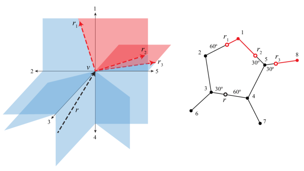
Figure 13: The ruffle (in red) of vertex $v\in\mathcal{K}$ with respect to incoming ray $r$, shown in $\cal K$ (left) and in the link graph $G_{v}$ (right). The boundary rays of the ruffle are $r_{1}$, $r_{2}$, and $r_{3}$.

Consider one region of the shortest path map, and the set, $C$, of shortest paths to points in the region. The paths in $C$ all go through the same sequence, $S_{C}$, of faces and edges and vertices. Let $v$ be the last vertex in the sequence $S_{C}$ (possibly $v=s$). There is a unique geodesic path from $s$ to $v$, and all the paths of $C$ traverse this same path from $s$ to $v$. After that, the points of the paths of $C$ all lie in the ruffle of $v$. Since the paths traverse the same sequence of edges and faces they can be laid out in the plane to form a cone with apex $v$. See Figure 14. Observe that the boundary rays of the cone may or may not lie in the set $C$. If the boundary of the cone is the boundary of the ruffle of $v$ then it is included in $C$; but if the boundary of the cone is determined by another vertex, then beyond that vertex, the boundary is not included. Note however, that the boundary ray is a shortest path—just not of the same combinatorial type since it goes through another vertex.

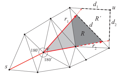
Figure 14: The structure of shortest paths to one region $R$ (shown darkly shaded) of the shortest path map. The set $C$ of shortest paths to points in the region forms a path $\sigma(s,v)$ together with a cone (lightly shaded) with apex $v$ bounded by rays $r_{1}$ and $r_{2}$. Region $R$ is closed on the $r_{1}$ boundary and open on the $r_{2}$ boundary. Shortest paths exit $R$ through segment $d$. The figure shows one region $R^{\prime}$ of the shortest path map beyond $d$. Shortest paths exit $R^{\prime}$ through two segments $d_{1}$ and $d_{2}$ and a vertex $u$. Note that the angles of the triangles incident to $v$ are not drawn accurately since they should sum to more than $2\pi$.

5.1.1 Computing the shortest path map

We will show that if the shortest path map has $M$ regions, then it can be computed in time $O(M)$. Regions of the shortest path map may have dimension 0, 1, or 2. Each 2-dimensional region of the shortest path map is bounded by: two boundary rays; a vertex or a segment of an edge through which shortest paths enter the region; and one or two segments of edges and possibly a vertex through which shortest paths exit the region. See Figure 14. With each region, we will store its boundary rays and vertices/segments. Each vertex of the complex is a 0-dimensional region of the shortest path map. An edge may form a 1-dimensional region of the shortest path map (for example any edge $(v,w)$ inside the ruffle of $v$).

The algorithm builds the regions of the shortest path map working outwards from $s$. In general, we will have a set of vertices and segments (portions of edges) that form the “frontier” of the known regions, and at each step of the algorithm, we will advance the known regions beyond one frontier vertex or segment.

The algorithm is initialized as follows. Assume that $s$ is a vertex of the complex (if necessary, by triangulating the face containing $s$ or the neighbouring faces if $s$ is on an edge). Each edge incident to $s$ becomes a region of the shortest path map. Each face $f$ incident to $s$ becomes a region of the shortest path map with the two edges of $f$ that are incident to $s$ as its boundary rays. The two vertices of $f$ different from $s$ enter the frontier, along with the edge of $f$ not incident to $s$.

At each step of the algorithm we take one vertex or segment out of the frontier set and we find all the regions for which shortest paths enter through this vertex or segment.

Consider first the case of removing segment $d$ from the frontier. We wish to find the regions of the shortest path map for which shortest paths enter through segment $d$. If segment $d$ lies in edge $e$, then the faces containing the new regions are those incident to $e$, not including the face from which shortest paths arrive at $d$. (See segment $d$ and region $R^{\prime}$ in Figure 14 for example.) Each such region $R^{\prime}$ gives rise to one or two segments and possibly a vertex through which shortest paths exit the region. We add these segments and vertex to the frontier. In case there is a vertex, $u$, (such as in Figure 14) we must find the shortest path to the vertex. This can be done by placing the boundary rays of $R^{\prime}$ in the plane, computing their point of intersection, $p$, and constructing the ray from $p$ to $u$. Note that we do not need to know the sequence of faces traversed by shortest paths to region $R^{\prime}$—local information suffices. This provides us with the shortest path to $u$ and also the boundary rays of the segments incident to $u$.

We next consider the case where a vertex $v$ is removed from the frontier. We must find the regions of the shortest path map for which shortest paths enter through vertex $v$. These lie in the ruffle of $v$. Knowing the shortest path $\sigma(s,v)$, we can search the link graph $G_{v}$ of $v$ to find all the boundary rays of the ruffle of $v$. Any edge incident to $v$ that lies in the ruffle forms a 1-dimensional region of the shortest path map, and we add its other endpoint to the frontier. For each face $f$ incident to $v$, we can identify the region of the shortest path map that lies in face $f$ and interior to the ruffle of $v$. We can also identify the segments and vertices through which shortest paths exit the new region, and add these to the frontier.

This completes the high-level description of the algorithm. We spend constant time per region of the shortest path map, plus $O(n)$ time to search the faces incident to each vertex, for a total of $O(M)$.

If we want to use the shortest path map to answer shortest path queries, we also need a way to locate, given a target point $t$ that lies in face $f$, which region of the shortest path map contains $t$. This necessitates building a search structure for the shortest path regions that face $f$ is partitioned into, which takes more time and space. (Results of Mount [49] might give a solution better than the obvious one for this.) We will not pursue this solution because we will present an alternative solution in Section 5.2.

5.1.2 Properties of the shortest path map

For our remaining results, we need some properties of shortest paths in a 2D CAT(0) complex.

We begin with the observation that shortest path rays diverge in any face, i.e., if we place the face in the plane and extend the two rays backwards, they meet. This is obvious (see Figure 14) for rays in one region of the shortest path map, and follows more generally from the fact that regions of the shortest path map partition any face.

Observation 1.

Any two shortest path rays in a face diverge.

Lemma 13.

Let $e$ be an edge of a 2D CAT(0) complex. Either all the shortest paths to internal points of $e$ travel along $e$, or they all reach $e$ from one incident face.

Proof.

If the shortest path to some internal point $p$ of edge $e$ travels along $e$ (i.e. arrives at $p$ from one of the endpoints of $e$), then so do the shortest paths to all internal points of $e$.

Otherwise shortest paths to internal points of $e$ arrive from faces incident to $e$. Consider the (finitely many) combinatorial types of shortest paths to points of $e$, and let $C_{1},C_{2},\ldots,C_{k}$ be the corresponding sets of shortest paths, ordered according to the order of points along $e$. We will prove that paths in all the $C_{i}$’s arrive at points of $e$ from the same incident face. For otherwise, there would be some $C_{i}$ and $C_{i+1}$ that arrive from different incident faces. Let $p$ be the point on $e$ that is the boundary between points reached by paths of $C_{i}$ and points reached by paths of $C_{i+1}$. Point $p$ must be reached by a ray in one of $C_{i}$ or $C_{i+1}$, say $C_{i+1}$. But observe that when $C_{i}$ is laid out in the plane, the boundary ray of its cone that is incident to $p$ is still a shortest path, and still arrives at $e$ from the same incident face as $C_{i}$ does. But this contradicts $C_{i+1}$ arriving from a different face. ∎

We next characterize how shortest paths can enter a face (a triangle) of the complex. See Figure 15.

Lemma 14.

Shortest paths enter a triangular face either through one edge, or one vertex, or one edge and an incident vertex, or two edges and their common vertex.

Proof.

We cannot have shortest paths entering a face from all three edges, nor from an edge and the opposite vertex, otherwise we would have shortest paths to two points on the same edge arriving from different faces, in contradiction to Lemma 13. ∎

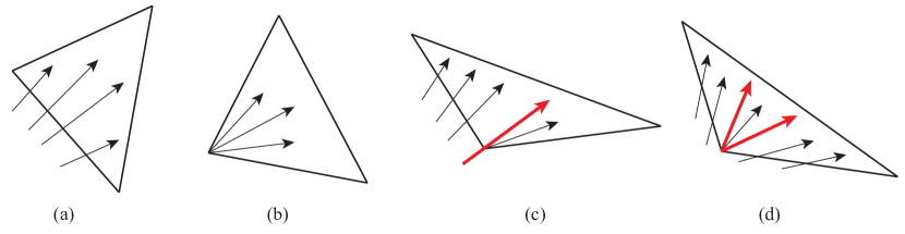
Figure 15: Shortest paths may enter a face through: (a) one edge (type E); (b) one vertex (type V); (c) one edge and an incident vertex (type EV); or (d) two edges and their common vertex (type EVE).

5.1.3 Size of the shortest path map

A boundary ray between adjacent regions of the shortest path map starts out as a boundary ray of the ruffle of some vertex. By Lemma 14, each face originates at most two such rays. In a general 2D CAT(0) complex, such a ray can bifurcate into two or more branches when it hits an edge that is incident to more than two faces. There is one branch for each new incident face. See Figure 17(a) for an example. The collection of all branches that originate from one boundary ray of a ruffle is called a boundary tree. Observe that it is a tree—no two branches can intersect because geodesic paths are unique. There are $O(n)$ boundary trees because each face originates at most two boundary trees. If the complex is a 2-manifold (i.e., every edge is in at most two faces) then no bifurcations can occur, so each boundary tree consists of only one branch, which implies that the size of the shortest path map is $O(n^{2})$. This was proved by Maftuleac [44] (where 2-manifold complexes are called “planar”), but we include a proof because we wish to observe a generalization.

Lemma 15 ([44]).

In a 2D CAT(0) complex that is a 2-manifold the size of the shortest path map is $O(n^{2})$.

Proof.

As noted above, every boundary tree consists of only one branch, or ray. If such a ray entered a face twice then the second entry would not be a shortest path, since we could short-cut across the face from the first entry. Therefore no ray enters a face twice, and the number of boundary tree branches cutting any face is $O(n)$. Then the number of regions of the shortest path map within one face is $O(n)$ and the overall number of regions is $O(n^{2})$. ∎

A general 2D CAT(0) complex may have the property that no two branches of one boundary tree cross the same face, in which case the shortest path map still has size $O(n^{2})$. We prove that this is the case for 2D CAT(0) rectangular complexes:

Lemma 16.

In a 2D CAT(0) rectangular complex, no two branches of one boundary tree can enter the same face, and from this it follows that the shortest path map has size $O(n^{2})$.

Proof.

Suppose, by contradiction, that two branches $r_{1}$ and $r_{2}$ of the same boundary tree enter a common face. Let $f$ be the first face along branch $r_{1}$ that they both enter. Let $f_{0}$ be the face just before the two branches diverge. The sequence of faces from $f_{0}$ to $f$ traversed by $r_{1}$ can be laid out in the plane so that $r_{1}$ forms a straight line. After a suitable rotation, the edges crossed by $r_{1}$ alternate between horizontal and vertical. Then the angle between $r_{1}$ and any horizontal edge it crosses is the same, say $\alpha$, and the angle between $r_{1}$ and any vertical edge it crosses is $\pi/2-\alpha$. See Figure 16. The same is true for $r_{2}$, and the angle $\alpha$ must be the same for $r_{1}$ and $r_{2}$ because the two rays match in face $f_{0}$. This means that $r_{1}$ and $r_{2}$ are parallel or perpendicular in $f$. If $r_{1}$ and $r_{2}$ are parallel then they do not diverge, which contradicts Observation 1. If $r_{1}$ and $r_{2}$ are perpendicular, then either they intersect in $f$, which is a contradiction, or there is some edge $e$ of $f$ that both rays pass through. If $r_{1}$ enters $f$ at edge $e$, then by Lemma 13, branch $r_{2}$ must reach $e$ from this same face, contradicting $f$ being the first face along branch $r_{1}$ that both branches enter. Thus $r_{1}$ must exit $f$ through edge $e$, and again by Lemma 13, $r_{2}$ must also exit through edge $e$. But then the two rays converge, which contradicts Observation 1.

Therefore the branches of one boundary tree enter a face at most once. Since there are $O(n)$ boundary trees, this means that the number of boundary tree branches cutting any face is $O(n)$. Then the number of regions of the shortest path map within one face is $O(n)$ and the overall number of regions is $O(n^{2})$. ∎

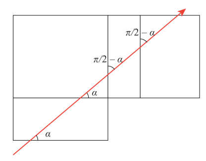
Figure 16: If a ray makes an angle of $\alpha$ with some horizontal edge in a 2D CAT(0) rectangular complex, then it makes the same angle $\alpha$ with every horizontal edge that it crosses, and it makes an angle $\pi/2-\alpha$ with every vertical edge that it crosses.

In a general 2D CAT(0) complex, two branches of one boundary tree may cross the same face—see Figure 17 for an example—and the size of the shortest path map may grow exponentially:

Proposition 17.

The size of the shortest path map of a 2D CAT(0) complex may be exponential in $n$, the number of faces.

Proof.

Figure 17(a–c) show how one boundary ray of a ruffle can bifurcate into two branches which then enter the same face $g_{2}$. Figure 17(d) shows how this process can be repeated. With each addition of three faces, $g_{i},f_{i}^{\prime}$, and $f_{i}^{\prime\prime}$, the number of branches doubles. Thus after adding $3n$ faces, the number of branches is $2^{n}$—so long as the angles are small enough that the process can be repeated $n$ times. To justify this, we need to be more precise about the angles.

For the initial set-up, let the angle between edge $e_{1}$ and the initial ray be $\alpha_{1}=\varepsilon$, with $\varepsilon$ to be chosen later. Define $\beta_{1}$, the angle between $e_{2}$ and [the extension of] $e_{1}$ to be $\beta_{1}=2\varepsilon$. More generally, define $\beta_{i}$, the angle between edge $e_{i+1}$ and [the extension of] $e_{i}$ to be $2^{i}\varepsilon$. Note that in our construction the sum of the angles of $f^{\prime}_{i},f^{\prime\prime}_{i}$ and $g_{i+1}$ at the point where they meet is $2\pi$, so the angle between $e_{i+1}$ and [the extension of] $e_{i}$ is well-defined.

We claim that in the general situation, as shown in Figure 18(a), we have an edge $e_{i}$ and a fan of $2^{i}$ pairs of branches that meet in pairs along $e_{i}$, and form an increasing sequence of angles from $\alpha_{1}$ to $\alpha_{i}=(2^{i}-1)\varepsilon$. We prove this by induction on $i$. It is true initially with $i=1$. For the induction step from $i$ to $i+1$, it suffices to examine the outer pair of branches, since they determine the two extreme rays intersecting $e_{i+1}$. Refer to Figure 18(b). From $\alpha_{i}=(2^{i}-1)\varepsilon$ and $\beta_{i}=2^{i}\varepsilon$, we calculate that the maximum angle between a branch and $e_{i+1}$ is $\alpha_{i+1}=(2^{i+1}-1)\varepsilon$ and the minimum angle between a branch and $e_{i+1}$ is $\alpha_{1}$. The remaining branches have slopes and intersection points on $e_{i+1}$ that lie between these two extremes. These $2^{i}$ branches are then reflected in $e_{i+1}$ to form a fan of $2^{i+1}$ pairs of branches, which completes the induction proof.

The induction step to $i+1$ can be carried out so long as $\beta_{i}+\alpha_{i}<\pi$. Thus, by choosing $\varepsilon<\pi/2^{n}$ we guarantee $\beta_{n-1}+\alpha_{n-1}<2^{n}\varepsilon<\pi$, and we can continue the branching process for $n$ steps. We note that this construction produces an exponential-sized shortest path map only by using $O(n)$ bits for the angles. ∎

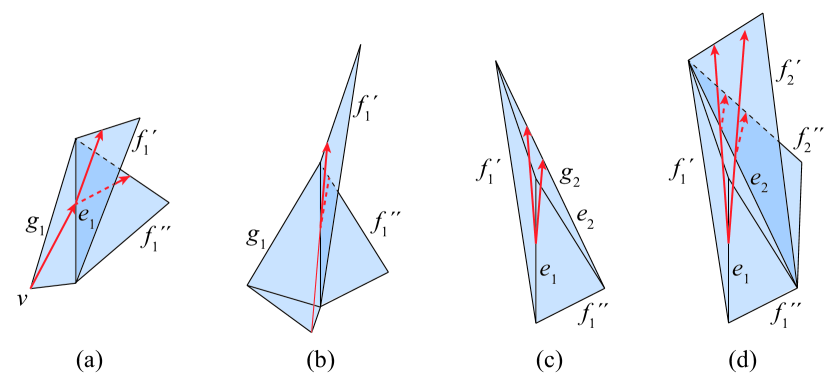
Figure 17: (a) A boundary ray of a ruffle (shown in red with arrows) originates from vertex $v$ in face $g_{1}$, and bifurcates when it reaches edge $e_{1}$, branching into two rays, one in face $f_{1}^{\prime}$ and one in face $f_{1}^{\prime\prime}$. (b) The same situation but with sharper angles. (c) The two resulting branches enter face $g_{2}$ that is incident to $f_{1}^{\prime}$ and $f_{1}^{\prime\prime}$, and arrive at edge $e_{2}$. Note that (b) and (c) show opposite sides of face $f_{1}^{\prime}$. (d) Two more faces $f_{2}^{\prime}$ and $f_{2}^{\prime\prime}$ are incident to edge $e_{2}$, so the two branches bifurcate into a total of four branches. In the next iteration, the four branches will enter a face $g_{3}$ incident to $f_{2}^{\prime}$ and $f_{2}^{\prime\prime}$. The process can be continued, and the number of rays doubles each time we add three faces.

Figure 18: A more detailed view of the angles used in the construction from Figure 17: (a) the general set-up; (b) the next step.

Note that an exponential size shortest path map does not preclude polynomial time algorithms for computing shortest paths. In the tree space and its generalization, orthant space, the shortest path map, and indeed the number of regions in a face, can have exponential size [52, 45], but there is still a polynomial time algorithm for computing geodesics in these spaces [53, 45].

5.2 The Last Step Shortest Path Map

Although the shortest path map for single-source shortest paths in a 2D CAT(0) complex may have exponential size, there is a structure, called the “last step shortest path map,” that has linear size and can be used to find the shortest path to a queried target point in time proportional to the combinatorial size of the path (i.e., the number of faces, edges, and vertices traversed by the path).

The last step shortest path map, first introduced in [24], partitions the space into regions where points $p$ and $q$ are in the same region if the shortest paths $\sigma(s,p)$ and $\sigma(s,q)$ have the same last vertex, edge, or face, i.e., the combinatorial type of the two paths matches on the last element. Thus, the last step shortest path map is a coarsening of the shortest path map. By Lemma 14 each face has one of the types shown in Figure 15, and is partitioned into one, two, or three regions. We store the type of each face, and for type EV and EVE faces we store the rays that partition the face based on the edge/vertex through which shortest paths enter.

For the purpose of answering shortest path queries, we store with each region of the last step shortest path map the last vertex, edge, or face with which shortest paths enter the region. We call this the incoming information (“in-info”) for the region. By Lemmas 13 and 14 the possible regions and possible in-info are as follows:

• a vertex $v$, with in-info a vertex $u$ (via edge $(u,v)$), or a face $f$

• an edge $e$, with in-info an endpoint $u$ of $e$, or a face $f$

• a face, partitioned into one, two, or three regions, each with in-info a vertex $u$ or an edge $e$

For any 2D CAT(0) complex the last step shortest path map has size $O(n)$. The incoming information also has size $O(n)$.

5.2.1 Answering shortest path queries using the last step shortest path map

We show that the last step shortest path map, together with the in-info described above, is sufficient to recover the path from $s$ to any point $t$ in time proportional to the number of faces and edges on the path. A query point $t$ is given as a vertex, or a point on an edge, or a point (in local coordinates) in a face. We find the path working backwards from $t$.

If $t$ is a vertex or a point on an edge and the in-info is a face, then we treat $t$ as a point in the face. For a point in a face, we test the partition of the face to determine which region contains $t$.

If the in-info for $t$’s region is a vertex $u$ then we replace $t$ by $u$ and recurse.

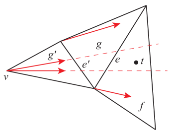
Figure 19: Finding the shortest path from $s$ to point $t$ in face $f$. In this example, $f$ is of type VE. Testing the ray of $f$, we find that the shortest path to $t$ enters from edge $e$ which has incoming face $g$ of type VE. Testing the rays of $g$, we find that the shortest path to $t$ enters from edge $e^{\prime}$ which has incoming face $g^{\prime}$ of type EVE. Finally, testing the rays of $g^{\prime}$ we find that the shortest path to $t$ comes from vertex $v$. We recursively find the shortest path to $v$.

Otherwise, $t$’s region is part of a face $f$, and in-info is an edge $e$. We place $f$ in the plane (arbitrarily) and enter the main loop of the algorithm (see Figure 19): Let $g$ be the incoming face for edge $e$. Attach triangle $g$ on the other side of edge $e$ of face $f$ in the plane. Note that the placement of $g$ is uniquely determined. If $g$ is of type V, we replace $t$ by the incoming vertex of $g$ and recurse. If $g$ is of type VE or type EVE we locate $t$ relative to the rays that partition $g$ (although $t$ is not in $g$ we just extend the rays to do the test). From this we can tell if the shortest path to $t$ goes through a vertex of $g$ or not. If it does, then we replace $t$ by that vertex and recurse. Otherwise the shortest path to $t$ enters $g$ through an edge, and we repeat the loop with the incoming face of that edge.

This algorithm finds the shortest path from $s$ to $t$ in time proportional to the number of triangles and edges on the path. In the worst case this is $O(n)$.

5.2.2 Computing the last step shortest path map

We do not know how to compute the last step shortest path map in polynomial time. More broadly, we do not know of a polynomial-time algorithm to compute shortest paths in a 2D CAT(0) complex. On the other hand, the problem does not seem to be amenable to NP-hardness proofs like the ones for shortest paths in 3D Euclidean space with polyhedral obstacles [15], or for shortest paths that visit a sequence of non-convex polygons in the plane [24]. Furthermore, we have the example of orthant spaces as CAT(0) complexes with exponential shortest path maps, but a polynomial time algorithm for computing shortest paths [45].

It is tempting to think that the last step shortest path map can be computed in a straight-forward way by propagating incoming information outward from the source. The trouble with this approach is that faces of type EVE need incoming information from two edges. This can result in dependencies that form a cycle, with each edge/face waiting for incoming information from some other face/edge. See Figure 20 for an example.

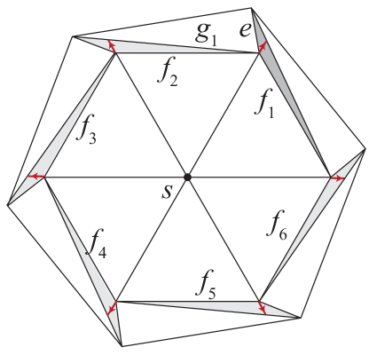
Figure 20: A cycle of incoming information in a 2D CAT(0) complex that lies in the plane. Face $f_{1}$ (darkly shaded) is of type EVE with incoming edge $e$, which has incoming face $g_{1}$, which depends on incoming information from face $f_{2}$. Similarly, each face $f_{i}$ (lightly shaded) depends on incoming information from face $f_{i+1}$, and $f_{6}$ depends on incoming information from face $f_{1}$, which creates a cycle. The red arrows indicate the ruffles of the vertices.

We end this section with one positive, though weak, result. The last step shortest path map can be computed from the shortest path map in time $O(M)$, where $M$ is the size of the shortest path map. For each edge, we can identify the incoming edge or face from any of the shortest path regions containing portions of the edge (by Lemma 13 these all give the same information). Since we have the shortest path to each vertex $v$, we can recover or recompute the boundary rays of the ruffle of $v$, which gives us the type (E, V, EV, or EVE) of each face incident to $v$, and the incoming information for the face.

We summarize the implications for special cases of the single-source shortest path problem in 2D CAT(0) complexes:

Proposition 18.

For a 2D CAT(0) complex that is a 2-manifold or is rectangular, we can solve the single-source shortest path problem using $O(n^{2})$ time and space to produce a structure (the last step shortest path map) of size $O(n)$ that allows us to answer shortest path queries in time proportional to the number of triangles and edges on the path.

6 Conclusions

We have given an algorithm for computing the closure of the convex hull of a set of points in a 2D CAT(0) polyhedral complex with a single vertex. Our algorithm relies on linear programming. The main open questions are:

• Is there a polynomial-time combinatorial algorithm to compute the convex hull of a set of points in a 2D CAT(0) polyhedral complex with a single vertex?

• Is such a convex hull closed? We conjecture that it is.

• Does the simple iterative approach of computing successive skeletons $S_{k}$ run in polynomial time? I.e., does $S_{k}=S_{k+1}$ for some $k$ that is polynomially bounded in the size of the complex (Conjecture 1)?

• Is there a polynomial time algorithm to test if given point is in the convex hull of a given point set in a CAT(0) polyhedral complex? This may be easier than computing the convex hull, and would be sufficient for most applications, including computing a geometric centre by peeling convex hulls.

• Does our linear programming solution extend to 2D CAT(0) complexes with more than one vertex, or to single-vertex higher dimensional CAT(0) complexes? The latter problem seems hard because in 3D and beyond the boundary between two maximal cells has dimension at least 2, and it is not clear that the intersection of the convex hull with a boundary face is even a polytope.

For the single-source shortest path problem in a 2D CAT(0) complex, we have shown that the shortest path map may have exponential size, and that the last step shortest path map is a better alternative. The main open questions are:

• Can the last step shortest path map be computed in polynomial time?

• Is the shortest path problem NP-hard for 2D CAT(0) complexes?

7 Acknowledgements

The authors thank Sean Skwerer for the example showing convex hulls of 3 points can be 3-dimensional (Figure 7), and Aasa Feragen, Steve Marron, Ezra Miller, Vinayak Pathak, Scott Provan, and Sean Skwerer for helpful discussions about convex hulls in tree space. We are extremely grateful to some incredibe anonymous reviewers, who greatly improved the paper and caught an error.

MO acknowledges the support of the Fields Institute. Research of all authors was supported by NSERC, the Natural Sciences and Engineering Research Council of Canada.

References

- [1] I. Agol. The virtual Haken conjecture. Doc. Math 18:1045–1087, 2013. With an appendix by I. Agol, D. Groves, and J. Manning.
- [2] R. K. Ahuja, T. L. Magnanti, and J. B. Orlin. Network Flows: Theory, Algorithms, and Applications. Prentice Hall, Englewood Cliffs, NJ, 1993.
- [3] F. Ardila, M. Owen, and S. Sullivant. Geodesics in CAT(0) cubical complexes. Advances in Applied Mathematics 48(1):142–163, 2012, doi:10.1016/j.aam.2011.06.004.
- [4] H.-J. Bandelt, P. Forster, and A. Röhl. Median-joining networks for inferring intraspecific phylogenies. Molecular biology and evolution 16(1):37–48, 1999, doi:10.1093/oxfordjournals.molbev.a026036.
- [5] D. Barden and H. Le. The logarithm map, its limits and fréchet means in orthant spaces. Proceedings of the London Mathematical Society 117(4):751–789, 2018, doi:10.1112/plms.12149.
- [6] D. Barden, H. Le, and M. Owen. Limiting behaviour of Fréchet means in the space of phylogenetic trees. Annals of the Institute of Statistical Mathematics 70(1):99–129, 2018, doi:10.1007/s10463-016-0582-9.
- [7] J.-P. Barthélémy and J. Constantin. Median graphs, parallelism and posets. Discrete mathematics 111(1-3):49–63, 1993, doi:10.1016/0012-365X(93)90140-O.
- [8] M. Bačák. Computing medians and means in Hadamard spaces. SIAM Journal on Optimization 24(3):1542–1566, 2014, doi:10.1137/140953393.
- [9] M. Bačák. Convex analysis and optimization in Hadamard spaces. De Gruyter Series in Nonlinear Analysis and Applications 22. Walter de Gruyter GmbH & Co KG, 2014.
- [10] M. Berger. A panoramic view of Riemannian geometry. Springer Science & Business Media, 2003, doi:10.1007/978-3-642-18245-7.
- [11] L. J. Billera, S. P. Holmes, and K. Vogtmann. Geometry of the space of phylogenetic trees. Advances in Applied Mathematics 27(4):733–767, 2001, doi:10.1006/aama.2001.0759.
- [12] A. Borbély. Some results on the convex hull of finitely many convex sets. Proceedings of the American Mathematical Society 126(5):1515–1525, 1998, doi:10.1090/S0002-9939-98-04155-0.
- [13] B. H. Bowditch. Some results on the geometry of convex hulls in manifolds of pinched negative curvature. Commentarii Mathematici Helvetici 69(1):49–81, 1994, doi:10.1007/BF02564474.
- [14] M. R. Bridson and A. Haefliger. Metric spaces of non-positive curvature, vol. 319. Springer Science & Business Media, 2013, doi:10.1007/978-3-662-12494-9.
- [15] J. Canny and J. Reif. New lower bound techniques for robot motion planning problems. 28th Annual Symp. on Foundations of Computer Science(FOCS), pp. 49–60, 1987, doi:10.1109/SFCS.1987.42.
- [16] T. M. Chan. Optimal output-sensitive convex hull algorithms in two and three dimensions. Discrete & Computational Geometry 16(4):361–368, 1996, doi:10.1007/BF02712873.
- [17] B. Chazelle. Triangulating a simple polygon in linear time. Discrete & Computational Geometry 6:485–524, 1991, doi:10.1007/BF02574703.
- [18] B. Chazelle. An optimal convex hull algorithm in any fixed dimension. Discrete and Computational Geometry 10(1):377–409, 1993, doi:10.1007/BF02573985.
- [19] J. Chen and Y. Han. Shortest paths on a polyhedron, Part I: Computing shortest paths. International Journal of Computational Geometry & Applications 6(02):127–144, 1996, doi:10.1142/S0218195996000095.
- [20] V. Chepoi. Graphs of some CAT(0) complexes. Advances in Applied Mathematics 24(2):125–179, 2000, doi:10.1006/aama.1999.0677.
- [21] V. Chepoi, F. F. Dragan, and Y. Vaxès. Distance and routing labeling schemes for non-positively curved plane graphs. Journal of Algorithms 61(2):60–88, 2006, doi:10.1016/j.jalgor.2004.07.011.
- [22] V. Chepoi and D. Maftuleac. Shortest path problem in rectangular complexes of global nonpositive curvature. Computational Geometry 46(1):51–64, 2013, doi:10.1016/j.comgeo.2012.04.002.
- [23] G. B. Dantzig. Linear Programming and Extensions. Princeton University Press, 1963, doi:10.7249/R366.
- [24] M. Dror, A. Efrat, A. Lubiw, and J. S. Mitchell. Touring a sequence of polygons. Proceedings of the 35th Annual ACM Symposium on Theory of Computing (STOC), pp. 473–482, 2003, doi:10.1145/780542.780612.
- [25] M. Elder and J. McCammond. CAT(0) is an algorithmic property. Geometriae Dedicata 107(1):25–46, 2004, doi:10.1023/B:GEOM.0000049096.63639.e3.
- [26] J. Felsenstein. Confidence limits on phylogenies: an approach using the bootstrap. Evolution pp. 783–791, 1985, doi:10.1111/j.1558-5646.1985.tb00420.x.
- [27] P. Fletcher, J. Moeller, J. Phillips, and S. Venkatasubramanian. Horoball hulls and extents in positive definite space. Algorithms and Data Structures, pp. 386-398. Springer Berlin Heidelberg, Lecture Notes in Computer Science 6844, 2011, doi:10.1007/978-3-642-22300-6_33.
- [28] R. Ghrist and V. Peterson. The geometry and topology of reconfiguration. Advances in Applied Mathematics 38(3):302–323, 2007, doi:10.1016/j.aam.2005.08.009.
- [29] M. Gromov. Hyperbolic groups. Essays in Group Theory, pp. 75-263. Springer New York, Mathematical Sciences Research Institute Publications 8, 1987, doi:10.1007/978-1-4613-9586-7_3.
- [30] L. Guibas, J. Hershberger, D. Leven, M. Sharir, and R. E. Tarjan. Linear-time algorithms for visibility and shortest path problems inside triangulated simple polygons. Algorithmica 2(1-4):209–233, 1987, doi:10.1007/BF01840360.
- [31] L. J. Guibas and J. Hershberger. Optimal shortest path queries in a simple polygon. Journal of Computer and System Sciences 39(2):126 – 152, 1989, doi:10.1016/0022-0000(89)90041-X.
- [32] F. Haglund and D. T. Wise. Special cube complexes. Geometric and Functional Analysis 17(5):1551–1620, 2008, doi:10.1007/s00039-007-0629-4.
- [33] K. Hayashi. A polynomial time algorithm to compute geodesics in cat (0) cubical complexes. 45th International Colloquium on Automata, Languages, and Programming (ICALP 2018), 2018, doi:10.4230/LIPIcs.ICALP.2018.78.
- [34] J. Hershberger and J. Snoeyink. Computing minimum length paths of a given homotopy class. Computational Geometry 4(2):63–97, 1994, doi:10.1016/0925-7721(94)90010-8.
- [35] J. Hershberger and S. Suri. An optimal algorithm for euclidean shortest paths in the plane. SIAM J. Comput 28:2215–2256, 1997, doi:10.1137/S0097539795289604.
- [36] S. Holmes. Statistical approach to tests involving phylogenies. Mathematics of evolution and phylogeny. Oxford University Press, Oxford, UK pp. 91–120, 2005.
- [37] M. Ishaque and C. D. Tóth. Relative convex hulls in semi-dynamic arrangements. Algorithmica 68(2):448–482, 2014, doi:10.1007/s00453-012-9679-6.
- [38] N. Karmarkar. A new polynomial-time algorithm for linear programming. Proceedings of the sixteenth annual ACM symposium on Theory of computing, pp. 302–311, 1984, doi:10.1007/BF02579150.
- [39] L. G. Khachiyan. Polynomial algorithms in linear programming. USSR Computational Mathematics and Mathematical Physics 20(1):53–72, 1980, doi:10.1016/0041-5553(80)90061-0.
- [40] D. G. Kirkpatrick and R. Seidel. The ultimate planar convex hull algorithm? SIAM Journal on Computing 15(1):287–299, 1986, doi:10.1137/0215021.
- [41] D. Lee and F. P. Preparata. Euclidean shortest paths in the presence of rectilinear barriers. Networks 14(3):393–410, 1984, doi:10.1002/net.3230140304.
- [42] D.-T. Lee and B. J. Schachter. Two algorithms for constructing a Delaunay triangulation. International Journal of Computer and Information Sciences 9(3):219–242, 1980, doi:10.1007/BF00977785.
- [43] B. Lin, B. Sturmfels, X. Tang, and R. Yoshida. Convexity in tree spaces. SIAM Journal on Discrete Mathematics 31(3):2015–2038, 2017, doi:10.1137/16M1079841.
- [44] D. Maftuleac. Algorithms for distance problems in planar complexes of global nonpositive curvature. International Journal of Computational Geometry & Applications 24(01):1–38, 2014, doi:10.1142/S0218195914500010.
- [45] E. Miller, M. Owen, and J. S. Provan. Polyhedral computational geometry for averaging metric phylogenetic trees. Advances in Applied Mathematics 68:51–91, 2015, doi:10.1016/j.aam.2015.04.002.
- [46] J. S. Mitchell. Geometric shortest paths and network optimization. Handbook of Computational Geometry, pp. 633–701. Elsevier Science Publishers B.V. North-Holland, 1998.
- [47] J. S. Mitchell, D. M. Mount, and C. H. Papadimitriou. The discrete geodesic problem. SIAM Journal on Computing 16(4):647–668, 1987, doi:10.1137/0216045.
- [48] J. S. Mitchell, D. M. Mount, and C. H. Papadimitriou. The discrete geodesic problem. SIAM Journal on Computing 16(4):647–668, 1987, doi:10.1137/0216045.
- [49] D. M. Mount. Storing the subdivision of a polyhedral surface. Discrete & Computational Geometry 2(1):153–174, 1987, doi:10.1007/BF02187877.
- [50] T. M. Nye. An algorithm for constructing principal geodesics in phylogenetic treespace. Computational Biology and Bioinformatics, IEEE/ACM Transactions on 11(2):304–315, 2014, doi:10.1109/TCBB.2014.2309599.
- [51] T. M. Nye, X. Tang, G. Weyenberg, and R. Yoshida. Principal component analysis and the locus of the fréchet mean in the space of phylogenetic trees. Biometrika 104(4):901–922, 2017, doi:10.1093/biomet/asx047.
- [52] M. Owen. Computing geodesic distances in tree space. SIAM Journal on Discrete Mathematics 25(4):1506–1529, 2011, doi:10.1137/090751396.
- [53] M. Owen and J. S. Provan. A fast algorithm for computing geodesic distances in tree space. IEEE/ACM Transactions on Computational Biology and Bioinformatics (TCBB) 8(1):2–13, 2011, doi:10.1109/TCBB.2010.3.
- [54] F. Ronquist and J. P. Huelsenbeck. MrBayes 3: Bayesian phylogenetic inference under mixed models. Bioinformatics 19(12):1572–1574, 2003, doi:10.1093/bioinformatics/btg180.
- [55] M. Sageev. Ends of group pairs and non-positively curved cube complexes. Proceedings of the London Mathematical Society 3(3):585–617, 1995, doi:10.1112/plms/s3-71.3.585.
- [56] R. Seidel. Convex hull computations. Handbook of Discrete and Computational Geometry (2nd edition), pp. 495–512. CRC Press, Inc., 2004, doi:10.1201/9781420035315.pt3.
- [57] G. Toussaint. An optimal algorithm for computing the relative convex hull of a set of points in a polygon. Signal Processing III: Theories and Applications, Proc. EURASIP-86, Part 2, pp. 853–856, 1986.
- [58] G. Toussaint. Computing geodesic properties inside a simple polygon. Rev. Intell. Artif. 3:9–42, 1989.
- [59] J. W. Tukey. Mathematics and the picturing of data. Proceedings of the International Congress of Mathematicians, vol. 2, pp. 523–531, 1975, doi:10.1090/S0002-9939-96-03657-X.
- [60] A. Willis. Confidence sets for phylogenetic trees. Journal of the American Statistical Association 114(525):235–244, 2019, doi:10.1080/01621459.2017.1395342.
- [61] G. U. Yule. A mathematical theory of evolution, based on the conclusions of Dr. JC Willis, FRS. Philosophical Transactions of the Royal Society of London. Series B, Containing Papers of a Biological Character pp. 21–87, 1925, doi:10.1098/rstb.1925.0002.