Structure of the preconditioned system in various preconditioned conjugate gradient squared algorithms

Abstract

An improved preconditioned conjugate gradient squared (PCGS) algorithm has recently been proposed, and it performs much better than the conventional PCGS algorithm. In this paper, the improved PCGS algorithm is verified as a coordinative to the left-preconditioned system, and it has the advantages of both the conventional and the left-PCGS; this is done by comparing, analyzing, and executing numerical examinations of various PCGS algorithms, including another improved one. We show that the direction of the preconditioned system for the CGS method is determined by the operations of $\alpha_{k}$ and $\beta_{k}$ in the PCGS algorithm. By comparing the logical structures of these algorithms, we show that the direction of the preconditioned system can be switched by the construction and setting of the initial shadow residual vector.

Keywords: Congruence of preconditioning conversion, Direction of preconditioned system, Preconditioned Krylov subspace, Improved PCGS

1 Introduction

The conjugate gradient squared (CGS) [12] is one of various methods used to solve systems of linear equations

(1.1) $$A\mbox{\boldmath{$x$}} = \mbox{\boldmath{$b$}},$$

where the coefficient matrix $A$ of size $n\times n$ is usually nonsymmetric, $x$ is the solution vector, and $b$ is the right-hand side (RHS) vector.

The CGS is a bi-Lanczos method that belongs to the class of Krylov subspace methods. Bi-Lanczos-type methods are derived from the bi-conjugate gradient (BiCG) method [4, 9], which assumes the existence of a dual system $A^{\rm T}\mbox{\boldmath{$x$}}^{\sharp}=\mbox{\boldmath{$b$}}^{\sharp}$ (we will refer to this as the “shadow system”). Bi-Lanczos-type algorithms have the advantage of requiring less memory than do Arnoldi-type algorithms, which is another class of Krylov subspace methods. Furthermore, a variety of bi-Lanczos-type algorithms, such as the bi-conjugate gradient stabilized (BiCGStab) method [14] and the generalized product-type method based on the BiCG (GPBiCG) [15], have been constructed by adopting the idea behind the derivation of the CGS. Various iterative methods, including bi-Lanczos-type algorithms, are often used following a preconditioning operation that is used to improve the properties of the linear equations. Such algorithms are called preconditioned algorithms; for example, the preconditioned CGS (PCGS). Therefore, it is very important to study the properties of the PCGS so that its performance can be improved.

Generally, the degree $k$ of the Krylov subspace generated by $A$ and $\mbox{\boldmath{$r$}}_{0}$ is expressed as ${\cal K}_{k}\left(A,\mbox{\boldmath{$r$}}_{0}\right)$ $={\rm span}\left\{\mbox{\boldmath{$r$}}_{0},A\mbox{\boldmath{$r$}}_{0},A^{2}\mbox{\boldmath{$r$}}_{0},\cdots,A^{k-1}\mbox{\boldmath{$r$}}_{0}\right\}$, where $\mbox{\boldmath{$r$}}_{0}$ is the initial residual vector $\mbox{\boldmath{$r$}}_{0}=\mbox{\boldmath{$b$}}-A\mbox{\boldmath{$x$}}_{0}$, and $\mbox{\boldmath{$x$}}_{0}$ is the initial guess at the solution. The Krylov subspace ${\cal K}_{k}\left(A,\mbox{\boldmath{$r$}}_{0}\right)$ generated by the $k$-th iteration forms the structure of $\mbox{\boldmath{$x$}}_{k}\in\mbox{\boldmath{$x$}}_{0}+{\cal K}_{k}\left(A,\mbox{\boldmath{$r$}}_{0}\right)$, where $\mbox{\boldmath{$x$}}_{k}$ is the approximate solution vector (or simply the “solution vector”). However, for a given preconditioned Krylov subspace method, there are various different algorithms that can be used for the preconditioning conversion. In such cases, the structure of the approximate solution formed by the Krylov subspace is often different for different algorithms, and the performance of these various algorithms can also differ substantially [7].

An improved PCGS algorithm has been proposed [7]. Reference [7] shows that this improved algorithm has many advantages over the conventional PCGS algorithms [1, 11, 14]. In this paper, a variety of PCGS algorithms are discussed. We begin by considering two typical PCGS algorithms, and we analyze the mathematical structure with respect to and in connection with the Krylov subspace. In particular, we define and consider the direction of the preconditioned system of these PCGS algorithms. We then perform the same analysis for two improved PCGS algorithms, one of which was mentioned above [7], and the other is presented in the present paper. However, we note that it is not our purpose to propose a new algorithm, but to analyze the improved PCGS algorithms by comparing the logical structures and the numerical results of four different PCGS algorithms.

In this paper, when we refer to a preconditioned algorithm, we mean one that uses a preconditioning operator $M$ or a preconditioning matrix, and by preconditioned system, we mean one that has been converted by some operator(s) based on $M$. These terms never indicate the algorithm for the preconditioning operation itself, such as incomplete LU decomposition or by using the approximate inverse. For example, under a preconditioned system, the original linear system (1.1) becomes

(1.2) $$\tilde{A}\tilde{\mbox{\boldmath{$x$}}}=\tilde{\mbox{\boldmath{$b$}}},$$

(1.3) $$\tilde{A}=M^{-1}_{L}AM^{-1}_{R},\;\;\tilde{\mbox{\boldmath{$x$}}}=M_{R}\mbox{\boldmath{$x$}},\;\;\tilde{\mbox{\boldmath{$b$}}}=M^{-1}_{L}\mbox{\boldmath{$b$}},$$

with the preconditioner $M=M_{L}M_{R}$ ($M\approx A$). In this paper, the matrix and the vector under the preconditioned system are indicated by a tilde ($\;\tilde{}\;$). However, the conversions in (1.2) and (1.3) are not implemented directly; rather, we construct the preconditioned algorithm that is equivalent to solving (1.2).

This paper is organized as follows. Section 2 provides various preconditioned CGS algorithms. In particular, we consider the right- and left-directions of the preconditioned systems for CGS algorithms. The improved PCGS algorithms are shown to be coordinative to the left-preconditioned system. Section 3 discusses the difference between the direction of a preconditioning conversion and the direction of a preconditioned system. We show that preconditioning conversions are congruent for PCGS algorithms, and we provide some examples in which the direction of the preconditioned system for the CGS is switched. In Section 4, we present some numerical results to illustrate the convergence properties of the various PCGS algorithms discussed in Section 2, and we illustrate the effect of switching the direction of the preconditioned system for the CGS algorithm in Section 3. Finally, our conclusions are presented in Section 5.

2 Analyses of various PCGS algorithms

In this section, four kinds of PCGS algorithms are analyzed. These PCGS algorithms can be derived as follows.

Algorithm 1. CGS under preconditioned system:

$\tilde{\mbox{\boldmath{$x$}}}_{0}$ is the initial guess, $\;\tilde{\mbox{\boldmath{$r$}}}_{0}=\tilde{\mbox{\boldmath{$b$}}}-\tilde{A}\tilde{\mbox{\boldmath{$x$}}}_{0}$, set $\;\beta^{\rm PCGS}_{-1}=0$,
$\left(\tilde{\mbox{\boldmath{$r$}}}^{\sharp}_{0},\tilde{\mbox{\boldmath{$r$}}}_{0}\right)\neq 0$, e.g., $\tilde{\mbox{\boldmath{$r$}}}^{\sharp}_{0}=\tilde{\mbox{\boldmath{$r$}}}_{0},\;$
For $k=0,1,2,\cdots,$ until convergence, Do:

$$\tilde{\mbox{\boldmath{$u$}}}_{k}=\tilde{\mbox{\boldmath{$r$}}}_{k}+\beta^{\rm PCGS}_{k-1}\tilde{\mbox{\boldmath{$q$}}}_{k-1},$$

$$\tilde{\mbox{\boldmath{$p$}}}_{k}=\tilde{\mbox{\boldmath{$u$}}}_{k}+\beta^{\rm PCGS}_{k-1}\left(\tilde{\mbox{\boldmath{$q$}}}_{k-1}+\beta^{\rm PCGS}_{k-1}\tilde{\mbox{\boldmath{$p$}}}_{k-1}\right),$$

$$\alpha^{\rm PCGS}_{k}=\frac{\left(\tilde{\mbox{\boldmath{$r$}}}^{\sharp}_{0},\tilde{\mbox{\boldmath{$r$}}}_{k}\right)}{\left(\tilde{\mbox{\boldmath{$r$}}}^{\sharp}_{0},\tilde{A}\tilde{\mbox{\boldmath{$p$}}}_{k}\right)},$$

$$\tilde{\mbox{\boldmath{$q$}}}_{k}=\tilde{\mbox{\boldmath{$u$}}}_{k}-\alpha^{\rm PCGS}_{k}\tilde{A}\tilde{\mbox{\boldmath{$p$}}}_{k},$$

(2.1) $$\tilde{\mbox{\boldmath{$x$}}}_{k+1}=\tilde{\mbox{\boldmath{$x$}}}_{k}+\alpha^{\rm PCGS}_{k}\left(\tilde{\mbox{\boldmath{$u$}}}_{k}+\tilde{\mbox{\boldmath{$q$}}}_{k}\right),$$

$$\tilde{\mbox{\boldmath{$r$}}}_{k+1}=\tilde{\mbox{\boldmath{$r$}}}_{k}-\alpha^{\rm PCGS}_{k}\tilde{A}\left(\tilde{\mbox{\boldmath{$u$}}}_{k}+\tilde{\mbox{\boldmath{$q$}}}_{k}\right),$$

$$\beta^{\rm PCGS}_{k}=\frac{\left(\tilde{\mbox{\boldmath{$r$}}}^{\sharp}_{0},\tilde{\mbox{\boldmath{$r$}}}_{k+1}\right)}{\left(\tilde{\mbox{\boldmath{$r$}}}^{\sharp}_{0},\tilde{\mbox{\boldmath{$r$}}}_{k}\right)},$$

End Do

Any preconditioned algorithm can be derived by substituting the matrix with the preconditioner for the matrix with the tilde and the vectors with the preconditioner for the vectors with the tilde. Obviously, Algorithm 2 without the preconditioning conversion is the same as the CGS. If $\tilde{A}$ is a symmetric matrix and $\tilde{\mbox{\boldmath{$r$}}}^{\sharp}_{0}=\tilde{\mbox{\boldmath{$r$}}}_{0}$, then Algorithm 2 can be adapted while maintaining its symmetric property.

The case shown in (1.3) is called two-sided preconditioning, the case in which $M_{L}=M$ and $M_{R}=I$ is called left preconditioning, and the case in which $M_{L}=I$ and $M_{R}=M$ is called right preconditioning, where $I$ denotes the identity matrix. We now formally define these.

Definition 1

For the system and solution

(2.2) $$\tilde{A}\tilde{\mbox{\boldmath{$x$}}}=\tilde{\mbox{\boldmath{$b$}}},$$

(2.3) $$\tilde{A}=M^{-1}_{L}AM^{-1}_{R},\;\;\tilde{\mbox{\boldmath{$x$}}}=M_{R}\mbox{\boldmath{$x$}},\;\;\tilde{\mbox{\boldmath{$b$}}}=M^{-1}_{L}\mbox{\boldmath{$b$}},$$

we define the direction of a preconditioned system of linear equations as follows:

• The two-sided preconditioned system: Equation (1.3');

• The right-preconditioned system: $M_{L}=I$ and $M_{R}=M$ in (1.3');

• The left-preconditioned system: $M_{L}=M$ and $M_{R}=I$ in (1.3'),

where $M$ is the preconditioner $M=M_{L}M_{R}$ ($M\approx A$), and $I$ is the identity matrix.

Other vectors in the solution method are not preconditioned. The initial guess is given as $\mbox{\boldmath{$x$}}_{0}$, and $\tilde{\mbox{\boldmath{$x$}}}_{0}=M_{R}\mbox{\boldmath{$x$}}_{0}$.

The two-sided preconditioned system may be impracticable, but it is of theoretical interest.

The preconditioned system is different from the preconditioning conversion as the next definition. There are various ways of performing a preconditioning conversion, but the direction of the preconditioned system is uniquely defined.

Definition 2 (Congruence)

Let the term “all directions on preconditioning conversions” be a synthesis of the preconditioning conversion for “the two-sided direction”, “the right direction”, and “the left direction”, not only for the system and solution (1.2'), but also for other vectors in the solution method.

If all directions on the preconditioning conversions to the solution method are reduced to one and the same algorithm description, then we refer to this as “congruence” in the direction of the preconditioning conversion. Furthermore, the term “congruency” refers to the congruence property.

As an example of congruence, see the preconditioning conversion by (2.6), (2.9), and (2.10) for Algorithm 2.1.1 in Section 2.1.1.

Both the CGS and the PCGS extend the two-dimensional subspace in each iteration [2, 5]; therefore, the Krylov subspace ${\cal K}_{2k}(\tilde{A},\tilde{\mbox{\boldmath{$r$}}}_{0})$ generated by the $k$-th iteration forms the structure of

(2.2) $$\tilde{\mbox{\boldmath{$x$}}}_{k}\in\tilde{\mbox{\boldmath{$x$}}}_{0}+{\cal K}_{2k}(\tilde{A},\tilde{\mbox{\boldmath{$r$}}}_{0}).$$

The CGS method is derived from the BiCG method [12]. Now, the recurrence relations of the BiCG under the preconditioned system are

$$R_{0}(\tilde{\lambda}) = 1,\;\;P_{0}(\tilde{\lambda})=1,$$

(2.3) $$R_{k}(\tilde{\lambda}) = R_{k-1}(\tilde{\lambda})-\alpha^{\rm PBiCG}_{k-1}\tilde{\lambda}P_{k-1}(\tilde{\lambda}),$$

(2.4) $$P_{k}(\tilde{\lambda}) = R_{k}(\tilde{\lambda})+\beta^{\rm PBiCG}_{k-1}P_{k-1}(\tilde{\lambda}).$$

Here, $R_{k}(\tilde{\lambda})$ is the degree $k$ of the residual polynomial, and $P_{k}(\tilde{\lambda})$ is the degree $k$ of the probing direction polynomial, that is, $\tilde{\mbox{\boldmath{$r$}}}^{\rm BiCG}_{k}=R_{k}(\tilde{A})\tilde{\mbox{\boldmath{$r$}}}_{0}$ and $\tilde{\mbox{\boldmath{$p$}}}^{\rm BiCG}_{k}=P_{k}(\tilde{A})\tilde{\mbox{\boldmath{$r$}}}_{0}$. The CGS method under preconditioned system can be derived by introducing the idea of $\{R_{k}(\tilde{\lambda})\}^{2}$ and $\{P_{k}(\tilde{\lambda})\}^{2}$ [7, 12]. Then, we can represent the following relations between these polynomials and the vectors in Algorithm 2:

(2.5) $$\tilde{\mbox{\boldmath{$r$}}}_{k}=\{R_{k}(\tilde{A})\}^{2}\tilde{\mbox{\boldmath{$r$}}}_{0},\;\;\;\;\;\;\;\;\tilde{\mbox{\boldmath{$p$}}}_{k}=\{P_{k}(\tilde{A})\}^{2}\tilde{\mbox{\boldmath{$r$}}}_{0},$$

$$\tilde{\mbox{\boldmath{$u$}}}_{k}=P_{k}(\tilde{A})R_{k}(\tilde{A})\tilde{\mbox{\boldmath{$r$}}}_{0},\;\;\;\;\tilde{\mbox{\boldmath{$q$}}}_{k}=P_{k}(\tilde{A})R_{k+1}(\tilde{A})\tilde{\mbox{\boldmath{$r$}}}_{0}.$$

2.1 Two typical PCGS algorithms

In this subsection, we present two well-known and typical PCGS algorithms. One is a right-preconditioned system, although this is not always recognized, and the other is a left-preconditioned system. For each of these algorithms, we examine the mathematical structure with respect to and in connection with the Krylov subspace and the solution vector.

2.1.1 Conventional PCGS: Right-preconditioned CGS

This PCGS algorithm has been described in many manuscripts and numerical libraries; for example, see [1, 11, 14]. It is usually derived by the following preconditioning conversion:

(2.6) $$\tilde{A}=M^{-1}_{L}AM^{-1}_{R},\;\;\tilde{\mbox{\boldmath{$x$}}}_{k}=M_{R}\mbox{\boldmath{$x$}}_{k},\;\;\tilde{\mbox{\boldmath{$b$}}}=M^{-1}_{L}\mbox{\boldmath{$b$}},\;\;\tilde{\mbox{\boldmath{$r$}}}_{k}=M^{-1}_{L}\mbox{\boldmath{$r$}}_{k},\;\;$$

$$\tilde{\mbox{\boldmath{$r$}}}^{\sharp}_{0}=M^{\rm T}_{L}\mbox{\boldmath{$r$}}^{\flat}_{0},\;\;\tilde{\mbox{\boldmath{$p$}}}_{k}=M^{-1}_{L}\mbox{\boldmath{$p$}}_{k},\;\;\tilde{\mbox{\boldmath{$u$}}}_{k}=M^{-1}_{L}\mbox{\boldmath{$u$}}_{k},\;\;\tilde{\mbox{\boldmath{$q$}}}_{k}=M^{-1}_{L}\mbox{\boldmath{$q$}}_{k}.$$

Finally, Algorithm 2.1.1 is derived.

Algorithm 2. Conventional PCGS algorithm:

$\mbox{\boldmath{$x$}}_{0}$ is the initial guess, $\;\mbox{\boldmath{$r$}}_{0}=\mbox{\boldmath{$b$}}-A\mbox{\boldmath{$x$}}_{0},\;\;$ set $\;\beta_{-1}=0,$
$\left(\tilde{\mbox{\boldmath{$r$}}}^{\sharp}_{0},\tilde{\mbox{\boldmath{$r$}}}_{0}\right)=\left(\mbox{\boldmath{$r$}}^{\flat}_{0},\mbox{\boldmath{$r$}}_{0}\right)\neq 0$, e.g., $\mbox{\boldmath{$r$}}^{\flat}_{0}=\mbox{\boldmath{$r$}}_{0},\;$

For $k=0,1,2,\cdots,$ until convergence, Do:

$$\mbox{\boldmath{$u$}}_{k}=\mbox{\boldmath{$r$}}_{k}+\beta_{k-1}\mbox{\boldmath{$q$}}_{k-1},$$

$$\mbox{\boldmath{$p$}}_{k}=\mbox{\boldmath{$u$}}_{k}+\beta_{k-1}\left(\mbox{\boldmath{$q$}}_{k-1}+\beta_{k-1}\mbox{\boldmath{$p$}}_{k-1}\right),$$

$$\alpha_{k}=\frac{\left(\mbox{\boldmath{$r$}}^{\flat}_{0},\mbox{\boldmath{$r$}}_{k}\right)}{\left(\mbox{\boldmath{$r$}}^{\flat}_{0},AM^{-1}\mbox{\boldmath{$p$}}_{k}\right)},$$

$$\mbox{\boldmath{$q$}}_{k}=\mbox{\boldmath{$u$}}_{k}-\alpha_{k}AM^{-1}\mbox{\boldmath{$p$}}_{k},$$

(2.7) $$\mbox{\boldmath{$x$}}_{k+1}=\mbox{\boldmath{$x$}}_{k}+\alpha_{k}M^{-1}\left(\mbox{\boldmath{$u$}}_{k}+\mbox{\boldmath{$q$}}_{k}\right),$$

$$\mbox{\boldmath{$r$}}_{k+1}=\mbox{\boldmath{$r$}}_{k}-\alpha_{k}AM^{-1}\left(\mbox{\boldmath{$u$}}_{k}+\mbox{\boldmath{$q$}}_{k}\right),$$

$$\beta_{k}=\frac{\left(\mbox{\boldmath{$r$}}^{\flat}_{0},\mbox{\boldmath{$r$}}_{k+1}\right)}{\left(\mbox{\boldmath{$r$}}^{\flat}_{0},\mbox{\boldmath{$r$}}_{k}\right)},$$

End Do

The stopping criterion is

(2.8) $$\frac{\|\mbox{\boldmath{$r$}}_{k+1}\|}{\|\mbox{\boldmath{$b$}}\|}\leq\varepsilon.$$

The results of this algorithm can also be derived by the following conversion:

(2.9) $$\tilde{A}=AM^{-1},\;\;\tilde{\mbox{\boldmath{$x$}}}_{k}=M\mbox{\boldmath{$x$}}_{k},\;\;\tilde{\mbox{\boldmath{$b$}}}=\mbox{\boldmath{$b$}},\;\;\tilde{\mbox{\boldmath{$r$}}}_{k}=\mbox{\boldmath{$r$}}_{k},\;\;$$

$$\tilde{\mbox{\boldmath{$r$}}}^{\sharp}_{0}=\mbox{\boldmath{$r$}}^{\flat}_{0},\;\;\tilde{\mbox{\boldmath{$p$}}}_{k}=\mbox{\boldmath{$p$}}_{k},\;\;\tilde{\mbox{\boldmath{$u$}}}_{k}=\mbox{\boldmath{$u$}}_{k},\;\;\tilde{\mbox{\boldmath{$q$}}}_{k}=\mbox{\boldmath{$q$}}_{k}.$$

This is the same as using $M_{L}=I$ and $M_{R}=M$ in (2.6). Furthermore, this is the same as converting only $\tilde{A}$, $\tilde{\mbox{\boldmath{$x$}}}_{k}$, and $\tilde{\mbox{\boldmath{$b$}}}$, that is, the right-preconditioned system.

Furthermore, as an example for congruence in Definition 2, the results of this algorithm can also be derived by the following left-preconditioning conversion:

(2.10) $$\tilde{A}=M^{-1}A,\;\;\tilde{\mbox{\boldmath{$x$}}}_{k}=\mbox{\boldmath{$x$}}_{k},\;\;\tilde{\mbox{\boldmath{$b$}}}=M^{-1}\mbox{\boldmath{$b$}},\;\;\tilde{\mbox{\boldmath{$r$}}}_{k}=M^{-1}\mbox{\boldmath{$r$}}_{k},\;\;$$

$$\tilde{\mbox{\boldmath{$r$}}}^{\sharp}_{0}=M^{\rm T}\mbox{\boldmath{$r$}}^{\flat}_{0},\;\;\tilde{\mbox{\boldmath{$p$}}}_{k}=M^{-1}\mbox{\boldmath{$p$}}_{k},\;\;\tilde{\mbox{\boldmath{$u$}}}_{k}=M^{-1}\mbox{\boldmath{$u$}}_{k},\;\;\tilde{\mbox{\boldmath{$q$}}}_{k}=M^{-1}\mbox{\boldmath{$q$}}_{k}.$$

2.1.2 Left-preconditioned CGS

The following conversion can be used to derive another PCGS algorithm:

(2.11) $$\tilde{A}=M^{-1}A,\;\;\tilde{\mbox{\boldmath{$x$}}}_{k}=\mbox{\boldmath{$x$}}_{k},\;\;\tilde{\mbox{\boldmath{$b$}}}=M^{-1}\mbox{\boldmath{$b$}},\;\;\tilde{\mbox{\boldmath{$r$}}}_{k}=\mbox{\boldmath{$r$}}^{+}_{k},\;\;$$

$$\tilde{\mbox{\boldmath{$r$}}}^{\sharp}_{0}=\mbox{\boldmath{$r$}}^{\sharp}_{0},\;\;\tilde{\mbox{\boldmath{$p$}}}_{k}=\mbox{\boldmath{$p$}}^{+}_{k},\;\;\tilde{\mbox{\boldmath{$u$}}}_{k}=\mbox{\boldmath{$u$}}^{+}_{k},\;\;\tilde{\mbox{\boldmath{$q$}}}_{k}=\mbox{\boldmath{$q$}}^{+}_{k}.$$

This is the same as applying $M_{L}=M$ and $M_{R}=I$ to $\tilde{A}$, $\tilde{\mbox{\boldmath{$x$}}}_{k}$, and $\tilde{\mbox{\boldmath{$b$}}}$, that is, the left-preconditioned system.

Algorithm 3. Left-preconditioned CGS algorithm (Left-PCGS):

$\mbox{\boldmath{$x$}}_{0}$ is the initial guess, $\;\mbox{\boldmath{$r$}}^{+}_{0}=M^{-1}\left(\mbox{\boldmath{$b$}}-A\mbox{\boldmath{$x$}}_{0}\right),\;\;$ set $\;\beta_{-1}=0,$
$\left(\tilde{\mbox{\boldmath{$r$}}}^{\sharp}_{0},\tilde{\mbox{\boldmath{$r$}}}_{0}\right)=\left(\mbox{\boldmath{$r$}}^{\sharp}_{0},\mbox{\boldmath{$r$}}^{+}_{0}\right)\neq 0$, e.g., $\mbox{\boldmath{$r$}}^{\sharp}_{0}=\mbox{\boldmath{$r$}}^{+}_{0},\;$
For $k=0,1,2,\cdots,$ until convergence, Do:

$$\mbox{\boldmath{$u$}}^{+}_{k}=\mbox{\boldmath{$r$}}^{+}_{k}+\beta_{k-1}\mbox{\boldmath{$q$}}^{+}_{k-1},$$

$$\mbox{\boldmath{$p$}}^{+}_{k}=\mbox{\boldmath{$u$}}^{+}_{k}+\beta_{k-1}\left(\mbox{\boldmath{$q$}}^{+}_{k-1}+\beta_{k-1}\mbox{\boldmath{$p$}}^{+}_{k-1}\right),$$

$$\alpha_{k}=\frac{\left(\mbox{\boldmath{$r$}}^{\sharp}_{0},\mbox{\boldmath{$r$}}^{+}_{k}\right)}{\left(\mbox{\boldmath{$r$}}^{\sharp}_{0},M^{-1}A\mbox{\boldmath{$p$}}^{+}_{k}\right)},$$

$$\mbox{\boldmath{$q$}}^{+}_{k}=\mbox{\boldmath{$u$}}^{+}_{k}-\alpha_{k}M^{-1}A\mbox{\boldmath{$p$}}^{+}_{k},$$

$$\mbox{\boldmath{$x$}}_{k+1}=\mbox{\boldmath{$x$}}_{k}+\alpha_{k}\left(\mbox{\boldmath{$u$}}^{+}_{k}+\mbox{\boldmath{$q$}}^{+}_{k}\right),$$

$$\mbox{\boldmath{$r$}}^{+}_{k+1}=\mbox{\boldmath{$r$}}^{+}_{k}-\alpha_{k}M^{-1}A\left(\mbox{\boldmath{$u$}}^{+}_{k}+\mbox{\boldmath{$q$}}^{+}_{k}\right),$$

$$\beta_{k}=\frac{\left(\mbox{\boldmath{$r$}}^{\sharp}_{0},\mbox{\boldmath{$r$}}^{+}_{k+1}\right)}{\left(\mbox{\boldmath{$r$}}^{\sharp}_{0},\mbox{\boldmath{$r$}}^{+}_{k}\right)},$$

End Do

In this paper, $\mbox{\boldmath{$r$}}^{+}_{k}$ denotes the residual vector under the left-preconditioned system, its internal structure is $\mbox{\boldmath{$r$}}^{+}_{k}\equiv M^{-1}\mbox{\boldmath{$r$}}_{k}$, and this is the definition of $\mbox{\boldmath{$r$}}^{+}_{k}$. Note that $\mbox{\boldmath{$p$}}^{+}_{k}$, $\mbox{\boldmath{$u$}}^{+}_{k}$, and $\mbox{\boldmath{$q$}}^{+}_{k}$ achieve the same purpose. Here, $\mbox{\boldmath{$r$}}^{+}_{k}$ in Algorithm 2.1.2 provides different information to the residual vector $\mbox{\boldmath{$r$}}_{k}=\mbox{\boldmath{$b$}}-A\mbox{\boldmath{$x$}}_{k}$, and the stopping criterion is

(2.12) $$\frac{\|\mbox{\boldmath{$r$}}^{+}_{k+1}\|}{\|M^{-1}\mbox{\boldmath{$b$}}\|}\leq\varepsilon.$$

Note that this is also different from (2.8), and this is an example of incomplete judging, because $\mbox{\boldmath{$r$}}^{+}_{k+1}$ never provides important information about $\mbox{\boldmath{$b$}}-A\mbox{\boldmath{$x$}}_{k}$. It may be thought that this is a minor issue, but in a previous paper, we observed that the left-preconditioned system can result in a serious problem (see [6], and Appendix A).

This algorithm can also be derived by the following conversion:

(2.13) $$\tilde{A}=M^{-1}_{L}AM^{-1}_{R},\;\;\tilde{\mbox{\boldmath{$x$}}}_{k}=M_{R}\mbox{\boldmath{$x$}}_{k},\;\;\tilde{\mbox{\boldmath{$b$}}}=M^{-1}_{L}\mbox{\boldmath{$b$}},\;\;\tilde{\mbox{\boldmath{$r$}}}_{k}=M_{R}\mbox{\boldmath{$r$}}^{+}_{k},\;\;$$

$$\tilde{\mbox{\boldmath{$r$}}}^{\sharp}_{0}=M^{-{\rm T}}_{R}\mbox{\boldmath{$r$}}^{\sharp}_{0},\;\;\tilde{\mbox{\boldmath{$p$}}}_{k}=M_{R}\mbox{\boldmath{$p$}}^{+}_{k},\;\;\tilde{\mbox{\boldmath{$u$}}}_{k}=M_{R}\mbox{\boldmath{$u$}}^{+}_{k},\;\;\tilde{\mbox{\boldmath{$q$}}}_{k}=M_{R}\mbox{\boldmath{$q$}}^{+}_{k}.$$

If $M_{L}=M$ and $M_{R}=I$ are substituted into (2.13), then (2.11) is obtained.

2.1.3 Comparison between two typical PCGS algorithms

Here, we compare the conventional PCGS with the left-PCGS. We will focus on the mathematical structures with respect to and in connection with their Krylov subspaces and their solution vectors. Now, we define a polynomial ${\it\Phi}_{k}(\tilde{\lambda})$ symbolically as ${\it\Phi}_{k}(\tilde{\lambda})\equiv\alpha^{\rm PCGS}_{k}(P_{k}(\tilde{\lambda})R_{k}(\tilde{\lambda})+P_{k}(\tilde{\lambda})R_{k+1}(\tilde{\lambda}))$ using Eqs. (2.3) through (2.5), then

(2.14) $${\it\Phi}_{k}(\tilde{A})\tilde{\mbox{\boldmath{$r$}}}_{0}\equiv\alpha^{\rm PCGS}_{k}(\tilde{\mbox{\boldmath{$u$}}}_{k}+\tilde{\mbox{\boldmath{$q$}}}_{k})$$

of (2.1) in Algorithm 2, where $k$ on both sides indicates the $k$-th iteration. Then Eq. (2.2) on the relation among the structure of the solution vector, the polynomial and the Krylov subspace can be expressed as

(2.15) $$\tilde{\mbox{\boldmath{$x$}}}_{k}=\tilde{\mbox{\boldmath{$x$}}}_{k-1}+{\it\Phi}_{k-1}(\tilde{A})\tilde{\mbox{\boldmath{$r$}}}_{0}\;\in\;\tilde{\mbox{\boldmath{$x$}}}_{0}+{\cal K}_{2k}\left(\tilde{A},\tilde{\mbox{\boldmath{$r$}}}_{0}\right).$$

The conventional PCGS (Algorithm 2.1.1) is the right-preconditioned system, i.e., $\left(AM^{-1}\right)\left(M\mbox{\boldmath{$x$}}\right)=\mbox{\boldmath{$b$}}$, and $\mbox{\boldmath{$r$}}_{k}=\mbox{\boldmath{$b$}}-\left(AM^{-1}\right)\left(M\mbox{\boldmath{$x$}}_{k}\right)$, because this algorithm can be derived by the right-preconditioning conversion (2.9) and this satisfies the right-preconditioned system in Definition 1. Then the vectors in Algorithm 2.1.1 and each polynomial can be detailed using (2.5) as follows:

(2.16) $$\mbox{\boldmath{$r$}}^{\rm R}_{k}=\{R^{\rm R}_{k}(AM^{-1})\}^{2}\mbox{\boldmath{$r$}}_{0},\;\;\;\;\;\;\;\;\mbox{\boldmath{$p$}}^{\rm R}_{k}=\{P^{\rm R}_{k}(AM^{-1})\}^{2}\mbox{\boldmath{$r$}}_{0},$$

$$\mbox{\boldmath{$u$}}^{\rm R}_{k}=P^{\rm R}_{k}(AM^{-1})R^{\rm R}_{k}(AM^{-1})\mbox{\boldmath{$r$}}_{0},\;\;\;\;\mbox{\boldmath{$q$}}^{\rm R}_{k}=P^{\rm R}_{k}(AM^{-1})R^{\rm R}_{k+1}(AM^{-1})\mbox{\boldmath{$r$}}_{0}.$$

Here, the vectors and polynomials of the right-preconditioned system are denoted by superscript R, this is also true for the scalar parameters $\alpha_{k}$ and $\beta_{k}$. The relation between the solution vector and its polynomial ${\it\Phi}_{k-1}(\tilde{A})\tilde{\mbox{\boldmath{$r$}}}_{0}$ is

(2.17) $$M\mbox{\boldmath{$x$}}_{k}=M\mbox{\boldmath{$x$}}_{k-1}+{\it\Phi}^{\rm R}_{k-1}(AM^{-1})\mbox{\boldmath{$r$}}_{0},$$

where ${\it\Phi}^{\rm R}_{k-1}(AM^{-1})\mbox{\boldmath{$r$}}_{0}=\alpha^{\rm R}_{k-1}(\mbox{\boldmath{$u$}}^{\rm R}_{k-1}+\mbox{\boldmath{$q$}}^{\rm R}_{k-1})$. This means that the polynomial ${\it\Phi}^{\rm R}_{k-1}(AM^{-1})\mbox{\boldmath{$r$}}_{0}$ organizes the solution vector as $M\mbox{\boldmath{$x$}}_{k}$, not $\mbox{\boldmath{$x$}}_{k}$ directly, but $\mbox{\boldmath{$x$}}_{k}$ is calculated with corrections, as shown in (2.7) of Algorithm 2.1.1.

The left-PCGS (Algorithm 2.1.2) is the left-preconditioned system, i.e., $M^{-1}A\mbox{\boldmath{$x$}}=M^{-1}\mbox{\boldmath{$b$}}$, and $\mbox{\boldmath{$r$}}^{+}_{k}=M^{-1}\left(\mbox{\boldmath{$b$}}-A\mbox{\boldmath{$x$}}_{k}\right)$, because this algorithm can be derived by the left-preconditioning conversion (2.11) and satisfies the left-preconditioned system in Definition 1. Then the vectors in Algorithm 2.1.2 and each polynomial can be detailed using (2.5) as follows:

(2.18) $$\mbox{\boldmath{$r$}}^{\rm L}_{k}=\{R^{\rm L}_{k}(M^{-1}A)\}^{2}\mbox{\boldmath{$r$}}^{+}_{0},\;\;\;\;\;\;\;\;\mbox{\boldmath{$p$}}^{\rm L}_{k}=\{P^{\rm L}_{k}(M^{-1}A)\}^{2}\mbox{\boldmath{$r$}}^{+}_{0},$$

$$\mbox{\boldmath{$u$}}^{\rm L}_{k}=P^{\rm L}_{k}(M^{-1}A)R^{\rm L}_{k}(M^{-1}A)\mbox{\boldmath{$r$}}^{+}_{0},\;\;\;\;\mbox{\boldmath{$q$}}^{\rm L}_{k}=P^{\rm L}_{k}(M^{-1}A)R^{\rm L}_{k+1}(M^{-1}A)\mbox{\boldmath{$r$}}^{+}_{0}.$$

Here, the vectors and polynomials of the left-preconditioned system are denoted by superscript L, this is also true for the scalar parameters $\alpha_{k}$ and $\beta_{k}$. The relation between the solution vector and its polynomial ${\it\Phi}_{k-1}(\tilde{A})\tilde{\mbox{\boldmath{$r$}}}_{0}$ is

(2.19) $$\mbox{\boldmath{$x$}}_{k}=\mbox{\boldmath{$x$}}_{k-1}+{\it\Phi}^{\rm L}_{k-1}(M^{-1}A)\mbox{\boldmath{$r$}}^{+}_{0},$$

where ${\it\Phi}^{\rm L}_{k-1}(M^{-1}A)\mbox{\boldmath{$r$}}^{+}_{0}=\alpha^{\rm L}_{k-1}(\mbox{\boldmath{$u$}}^{\rm L}_{k-1}+\mbox{\boldmath{$q$}}^{\rm L}_{k-1})$. Therefore, the polynomial ${\it\Phi}^{\rm L}_{k-1}(M^{-1}A)\mbox{\boldmath{$r$}}^{+}_{0}$ organizes the solution vector directly as $\mbox{\boldmath{$x$}}_{k}$ (Algorithm 2.1.2).

These are summarized in Table  1.

Table 1: Summary of two typical PCGS algorithms.

	Structure of residual vector	Structure of the solution vector for each polynomial
Conventional (Alg. 2.1.1)	$\mbox{\boldmath{$r$}}_{k}=\mbox{\boldmath{$b$}}-(AM^{-1})(M\mbox{\boldmath{$x$}}_{k})$	$M\mbox{\boldmath{$x$}}_{k}=M\mbox{\boldmath{$x$}}_{k-1}+{\it\Phi}^{\rm R}_{k-1}(AM^{-1})\mbox{\boldmath{$r$}}_{0}$
Left-PCGS (Alg. 2.1.2)	$\mbox{\boldmath{$r$}}^{+}_{k}=M^{-1}\left(\mbox{\boldmath{$b$}}-A\mbox{\boldmath{$x$}}_{k}\right)$	$\mbox{\boldmath{$x$}}_{k}=\mbox{\boldmath{$x$}}_{k-1}+{\it\Phi}^{\rm L}_{k-1}(M^{-1}A)\mbox{\boldmath{$r$}}^{+}_{0}$

2.2 Improved preconditioned CGS algorithms

An improved PCGS algorithm has been proposed [7]. This algorithm retains some mathematical properties that are associated with the CGS derivation from the BiCG method under a non-preconditioned system. The improved PCGS algorithm from [7] will be referred to as “Improved1.” Another improved PCGS algorithm will be presented, and it will be referred to as “Improved2.” We note that Improved2 is mathematically equivalent to Improved1. The stopping criterion for both algorithms is (2.8).

2.2.1 Improved1 PCGS algorithm (Improved1) [7]

Improved1 can be derived from the following conversion:

(2.20) $$\tilde{A}=M^{-1}_{L}AM^{-1}_{R},\;\;\tilde{\mbox{\boldmath{$x$}}}_{k}=M_{R}\mbox{\boldmath{$x$}}_{k},\;\;\tilde{\mbox{\boldmath{$b$}}}=M^{-1}_{L}\mbox{\boldmath{$b$}},\;\;\tilde{\mbox{\boldmath{$r$}}}_{k}=M^{-1}_{L}\mbox{\boldmath{$r$}}_{k},\;$$

$$\tilde{\mbox{\boldmath{$r$}}}^{\sharp}_{0}=M^{-{\rm T}}_{R}\mbox{\boldmath{$r$}}^{\sharp}_{0},\;\;\tilde{\mbox{\boldmath{$p$}}}_{k}=M_{R}\mbox{\boldmath{$p$}}^{+}_{k},\;\;\tilde{\mbox{\boldmath{$u$}}}_{k}=M_{R}\mbox{\boldmath{$u$}}^{+}_{k},\;\;\tilde{\mbox{\boldmath{$q$}}}_{k}=M_{R}\mbox{\boldmath{$q$}}^{+}_{k}.$$

Algorithm 4. Improved PCGS algorithm (Improved1):

$\mbox{\boldmath{$x$}}_{0}$ is the initial guess, $\;\mbox{\boldmath{$r$}}_{0}=\mbox{\boldmath{$b$}}-A\mbox{\boldmath{$x$}}_{0},\;\;$ set $\;\beta_{-1}=0,$
$\left(\tilde{\mbox{\boldmath{$r$}}}^{\sharp}_{0},\tilde{\mbox{\boldmath{$r$}}}_{0}\right)=\left(\mbox{\boldmath{$r$}}^{\sharp}_{0},M^{-1}\mbox{\boldmath{$r$}}_{0}\right)\neq 0,\;\;$ e.g., $\mbox{\boldmath{$r$}}^{\sharp}_{0}=M^{-1}\mbox{\boldmath{$r$}}_{0},\;$
For $k=0,1,2,\cdots,$ until convergence, Do:

$$\mbox{\boldmath{$u$}}^{+}_{k}=M^{-1}\mbox{\boldmath{$r$}}_{k}+\beta_{k-1}\mbox{\boldmath{$q$}}^{+}_{k-1},$$

$$\mbox{\boldmath{$p$}}^{+}_{k}=\mbox{\boldmath{$u$}}^{+}_{k}+\beta_{k-1}\left(\mbox{\boldmath{$q$}}^{+}_{k-1}+\beta_{k-1}\mbox{\boldmath{$p$}}^{+}_{k-1}\right),$$

$$\alpha_{k}=\frac{\left(\mbox{\boldmath{$r$}}^{\sharp}_{0},M^{-1}\mbox{\boldmath{$r$}}_{k}\right)}{\left(\mbox{\boldmath{$r$}}^{\sharp}_{0},M^{-1}A\mbox{\boldmath{$p$}}^{+}_{k}\right)},$$

$$\mbox{\boldmath{$q$}}^{+}_{k}=\mbox{\boldmath{$u$}}^{+}_{k}-\alpha_{k}M^{-1}A\mbox{\boldmath{$p$}}^{+}_{k},$$

$$\mbox{\boldmath{$x$}}_{k+1}=\mbox{\boldmath{$x$}}_{k}+\alpha_{k}\left(\mbox{\boldmath{$u$}}^{+}_{k}+\mbox{\boldmath{$q$}}^{+}_{k}\right),$$

$$\mbox{\boldmath{$r$}}_{k+1}=\mbox{\boldmath{$r$}}_{k}-\alpha_{k}A\left(\mbox{\boldmath{$u$}}^{+}_{k}+\mbox{\boldmath{$q$}}^{+}_{k}\right),$$

$$\beta_{k}=\frac{\left(\mbox{\boldmath{$r$}}^{\sharp}_{0},M^{-1}\mbox{\boldmath{$r$}}_{k+1}\right)}{\left(\mbox{\boldmath{$r$}}^{\sharp}_{0},M^{-1}\mbox{\boldmath{$r$}}_{k}\right)},$$

End Do

2.2.2 Improved2 PCGS algorithm (Improved2)

Improved2 can be derived from the following conversion:

(2.21) $$\tilde{A}=M^{-1}_{L}AM^{-1}_{R},\;\;\tilde{\mbox{\boldmath{$x$}}}_{k}=M_{R}\mbox{\boldmath{$x$}}_{k},\;\;\tilde{\mbox{\boldmath{$b$}}}=M^{-1}_{L}\mbox{\boldmath{$b$}},\;\;\tilde{\mbox{\boldmath{$r$}}}_{k}=M^{-1}_{L}\mbox{\boldmath{$r$}}_{k},\;$$

$$\tilde{\mbox{\boldmath{$r$}}}^{\sharp}_{0}=M^{-{\rm T}}_{R}\mbox{\boldmath{$r$}}^{\sharp}_{0},\;\;\tilde{\mbox{\boldmath{$p$}}}_{k}=M^{-1}_{L}\mbox{\boldmath{$p$}}_{k},\;\;\tilde{\mbox{\boldmath{$u$}}}_{k}=M^{-1}_{L}\mbox{\boldmath{$u$}}_{k},\;\;\tilde{\mbox{\boldmath{$q$}}}_{k}=M^{-1}_{L}\mbox{\boldmath{$q$}}_{k}.$$

Note that this conversion is different than (2.20) for $\tilde{\mbox{\boldmath{$p$}}}_{k}$, $\tilde{\mbox{\boldmath{$u$}}}_{k}$, and $\tilde{\mbox{\boldmath{$q$}}}_{k}$.

Algorithm 5. Another improved PCGS algorithm (Improved2):

$\mbox{\boldmath{$x$}}_{0}$ is the initial guess, $\;\mbox{\boldmath{$r$}}_{0}=\mbox{\boldmath{$b$}}-A\mbox{\boldmath{$x$}}_{0},\;\;$ set $\;\beta_{-1}=0,$
$\left(\tilde{\mbox{\boldmath{$r$}}}^{\sharp}_{0},\tilde{\mbox{\boldmath{$r$}}}_{0}\right)=\left(\mbox{\boldmath{$r$}}^{\sharp}_{0},M^{-1}\mbox{\boldmath{$r$}}_{0}\right)\neq 0,\;\;$ e.g., $\mbox{\boldmath{$r$}}^{\sharp}_{0}=M^{-1}\mbox{\boldmath{$r$}}_{0}$,
For $k=0,1,2,\cdots,$ until convergence, Do:

$$\mbox{\boldmath{$u$}}_{k}=\mbox{\boldmath{$r$}}_{k}+\beta_{k-1}\mbox{\boldmath{$q$}}_{k-1},$$

$$\mbox{\boldmath{$p$}}_{k}=\mbox{\boldmath{$u$}}_{k}+\beta_{k-1}\left(\mbox{\boldmath{$q$}}_{k-1}+\beta_{k-1}\mbox{\boldmath{$p$}}_{k-1}\right),$$

$$\alpha_{k}=\frac{\left(M^{-{\rm T}}\mbox{\boldmath{$r$}}^{\sharp}_{0},\mbox{\boldmath{$r$}}_{k}\right)}{\left(M^{-{\rm T}}\mbox{\boldmath{$r$}}^{\sharp}_{0},AM^{-1}\mbox{\boldmath{$p$}}_{k}\right)},$$

$$\mbox{\boldmath{$q$}}_{k}=\mbox{\boldmath{$u$}}_{k}-\alpha_{k}AM^{-1}\mbox{\boldmath{$p$}}_{k},$$

$$\mbox{\boldmath{$x$}}_{k+1}=\mbox{\boldmath{$x$}}_{k}+\alpha_{k}M^{-1}\left(\mbox{\boldmath{$u$}}_{k}+\mbox{\boldmath{$q$}}_{k}\right),$$

$$\mbox{\boldmath{$r$}}_{k+1}=\mbox{\boldmath{$r$}}_{k}-\alpha_{k}AM^{-1}\left(\mbox{\boldmath{$u$}}_{k}+\mbox{\boldmath{$q$}}_{k}\right),$$

$$\beta_{k}=\frac{\left(M^{-{\rm T}}\mbox{\boldmath{$r$}}^{\sharp}_{0},\mbox{\boldmath{$r$}}_{k+1}\right)}{\left(M^{-{\rm T}}\mbox{\boldmath{$r$}}^{\sharp}_{0},\mbox{\boldmath{$r$}}_{k}\right)},$$

End Do

2.3 Analysis of the four kinds of PCGS algorithms

We will now analyze and compare the four PCGS algorithms presented above.

We split the residual vector of the left-PCGS (Algorithm 2.1.2) $\mbox{\boldmath{$r$}}^{+}_{k}$ into

(2.22) $$\mbox{\boldmath{$r$}}^{+}_{k}\mapsto M^{-1}\mbox{\boldmath{$r$}}_{k},\;\;(k=0,1,2,\cdots)$$

and give the necessary deformations; then, the left-PCGS (Algorithm 2.1.2) is reduced to Improved1 (Algorithm 2.2.1). Alternatively, we can derive Algorithm 2.1.2 from Algorithm 2.2.1 by substituting $M^{-1}\mbox{\boldmath{$r$}}_{k}$ for $\mbox{\boldmath{$r$}}^{+}_{k}$, that is, $\mbox{\boldmath{$r$}}^{+}_{k}\equiv M^{-1}\mbox{\boldmath{$r$}}_{k}$. By this means, we can explain the relationships between the four kinds of PCGS algorithms, as shown in Figure 1.

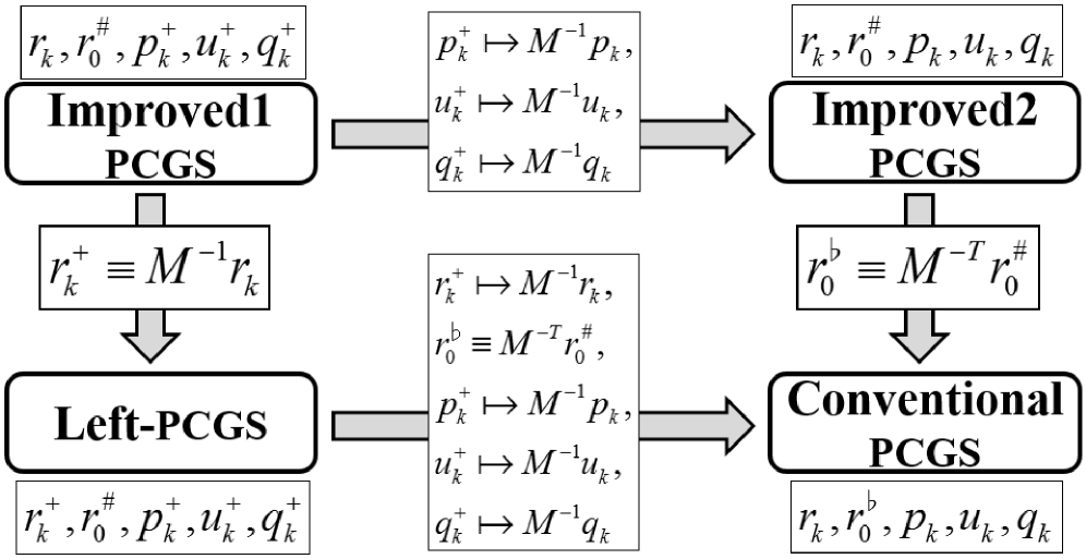
Figure 1: Relations between the four different PCGS algorithms. $\mapsto$ : Splitting left vector to right members (preconditioner and vector), $\equiv$ : Substituting left vector for right members.

In addition, if we apply (2.22) to (2.19) to obtain the structure of the polynomial ${\it\Phi}_{k}(\tilde{A})\tilde{\mbox{\boldmath{$r$}}}_{0}$ of Algorithm 2.1.2, then

$${\it\Phi}^{\rm L}_{k}(M^{-1}A)\mbox{\boldmath{$r$}}^{+}_{0}\;\;\mapsto\;\;{\it\Phi}^{\rm L}_{k}(M^{-1}A)M^{-1}\mbox{\boldmath{$r$}}_{0}=M^{-1}{\it\Phi}^{\rm L}_{k}(AM^{-1})\mbox{\boldmath{$r$}}_{0}.$$

Therefore, the system of Improved1 (Algorithm 2.2.1) is coordinative to that of the left-PCGS (Algorithm 2.1.2). Furthermore, the structure of the solution vector and the polynomial is

(2.23) $$\mbox{\boldmath{$x$}}_{k}=\mbox{\boldmath{$x$}}_{k-1}+{\it\Phi}^{\rm L}_{k-1}(M^{-1}A)\mbox{\boldmath{$r$}}^{+}_{0}\;\;\mapsto\;\;\mbox{\boldmath{$x$}}_{k}=\mbox{\boldmath{$x$}}_{k-1}+M^{-1}{\it\Phi}^{\rm L}_{k-1}(AM^{-1})\mbox{\boldmath{$r$}}_{0}.$$

Here, the polynomial is denoted as ${\it\Phi}^{\rm L}_{k-1}$, despite the preconditioned matrix being $AM^{-1}$ in the right-hand side of (2.23), because the direction of a preconditioned system is different from the direction of a preconditioning conversion (see Section 3).

Improved2 (Algorithm 2.2.2) is equivalent to Improved1. Both algorithms have important advantages over the left-PCGS, because their residual vector is $\mbox{\boldmath{$r$}}_{k}$, and their stopping criterion is (2.8), not $\|\mbox{\boldmath{$r$}}^{+}_{k+1}\|/\|M^{-1}\mbox{\boldmath{$b$}}\|$.

Table 2 shows the structure of the residual vector and the structure of the solution vector for each polynomial of the four PCGS algorithms.

Table 2: Summary of the four PCGS algorithms.

	Structure of residual vector	Structure of the solution vector for each polynomial
Conventional (Alg. 2.1.1)	$\mbox{\boldmath{$r$}}_{k}=\mbox{\boldmath{$b$}}-(AM^{-1})(M\mbox{\boldmath{$x$}}_{k})$	$M\mbox{\boldmath{$x$}}_{k}=M\mbox{\boldmath{$x$}}_{k-1}+{\it\Phi}^{\rm R}_{k-1}(AM^{-1})\mbox{\boldmath{$r$}}_{0}$
Left-PCGS (Alg. 2.1.2)	$\mbox{\boldmath{$r$}}^{+}_{k}=M^{-1}\left(\mbox{\boldmath{$b$}}-A\mbox{\boldmath{$x$}}_{k}\right)$	$\mbox{\boldmath{$x$}}_{k}=\mbox{\boldmath{$x$}}_{k-1}+{\it\Phi}^{\rm L}_{k-1}(M^{-1}A)\mbox{\boldmath{$r$}}^{+}_{0}$
Improved1 (Alg. 2.2.1)	$M^{-1}\mbox{\boldmath{$r$}}_{k}=$
Improved2 (Alg. 2.2.2)	$M^{-1}\left(\mbox{\boldmath{$b$}}-(AM^{-1})(M\mbox{\boldmath{$x$}}_{k})\right)$	$\mbox{\boldmath{$x$}}_{k}=\mbox{\boldmath{$x$}}_{k-1}+M^{-1}{\it\Phi}^{\rm L}_{k-1}(AM^{-1})\mbox{\boldmath{$r$}}_{0}$

In this summary, we see that the structures of the polynomial organizing the solution vector differ:

(2.24) $${\it\Phi}^{\rm R}_{k-1}(AM^{-1})\mbox{\boldmath{$r$}}_{0}\neq{\it\Phi}^{\rm L}_{k-1}(AM^{-1})\mbox{\boldmath{$r$}}_{0}.$$

In other words, ${\it\Phi}^{\rm R}_{k-1}(AM^{-1})\mbox{\boldmath{$r$}}_{0}$ of the conventional PCGS (right-preconditioned) system is different from ${\it\Phi}^{\rm L}_{k-1}(AM^{-1})\mbox{\boldmath{$r$}}_{0}$ of both improved PCGS (coordinative to the left-preconditioned) systems, because the scalar parameters $\alpha_{k}$ and $\beta_{k}$ are not equivalent (see Section 3.2) [7, 8]. This also affects the polynomial ${\it\Phi}_{k}(\tilde{A})\tilde{\mbox{\boldmath{$r$}}}_{0}$ for the following reason. Although, superficially, the solution vector for both the conventional PCGS (Algorithm 2.1.1) and Improved2 (Algorithm 2.2.2) have the same recurrence formula, i.e., $\mbox{\boldmath{$x$}}_{k+1}=\mbox{\boldmath{$x$}}_{k}+\alpha_{k}M^{-1}\left(\mbox{\boldmath{$u$}}_{k}+\mbox{\boldmath{$q$}}_{k}\right)$, each recurrence formula belongs to a different system because the components of the conventional PCGS are $\alpha^{\rm R}_{k}$, $\mbox{\boldmath{$u$}}^{\rm R}_{k}$, and $\mbox{\boldmath{$q$}}^{\rm R}_{k}$, and those of Improved2 are $\alpha^{\rm L}_{k}$, $\mbox{\boldmath{$u$}}^{\rm L}_{k}$, and $\mbox{\boldmath{$q$}}^{\rm L}_{k}$.

The structure of the residual vector of Improved1 (Algorithm 2.2.1) and Improved2 (Algorithm 2.2.2) appears as $M^{-1}\mbox{\boldmath{$r$}}_{k}=M^{-1}\left(\mbox{\boldmath{$b$}}-(AM^{-1})(M\mbox{\boldmath{$x$}}_{k})\right)$ in Table 2 because they are from the left-PCGS, and the structure of their polynomial is $M^{-1}{\it\Phi}^{\rm L}_{k-1}(AM^{-1})\mbox{\boldmath{$r$}}_{0}$.

Note that (2.24) will be confirmed in Section 3 and will be shown numerically in Section 4.

3 Congruence of preconditioning conversion, and direction of preconditioned system for the CGS

In the previous section, we defined the general direction of a preconditioned system for CGS (see Definition 1). However, the direction of a preconditioned system is different from the direction of a preconditioning conversion. We will show that the direction of a preconditioned system is switched by the construction of the initial shadow residual vector (ISRV).

3.1 Congruence of preconditioning conversion for the PCGS

Here, we consider the congruence of Definition 2 for the PCGS in the following proposition.

Proposition 1 (Congruency)

There is congruence to a PCGS algorithm in the direction of the preconditioning conversion.

Proof We have already shown instances of this. For example, Algorithm 2.1.1 can be derived by the two-sided conversion (2.6), and if $M_{L}=I$, $M_{R}=M$, and the conversion (2.6) is reduced to (2.9), then Algorithm 2.1.1 is derived. If $M_{L}=M$ and $M_{R}=I$, that is (2.10), then Algorithm 2.1.1 can be derived. The other preconditioned algorithms (Algorithms 2.1.2, 2.2.1, and 2.2.2) and their corresponding preconditioning conversions are also the same.   $\hfill\Box$

Although this property has been repeatedly discussed in the literature, it should be considered when evaluating the direction of a preconditioned system.

3.2 Direction of a preconditioned system and that of the PCGS

The direction of a preconditioned system is different from the direction of a preconditioning conversion.

Proposition 2

The direction of a preconditioned system is determined by the operations of $\alpha_{k}$ and $\beta_{k}$ in each PCGS algorithm. These intrinsic operations are based on biorthogonality $(\tilde{\mbox{\boldmath{$r$}}}^{\sharp}_{0},\tilde{\mbox{\boldmath{$r$}}}_{k})$ and biconjugacy $(\tilde{\mbox{\boldmath{$r$}}}^{\sharp}_{0},\tilde{A}\tilde{\mbox{\boldmath{$p$}}}_{k})$.

Proof The operations of biorthogonality and biconjugacy in each PCGS algorithm and the structure of the solution vector for each polynomial are shown below. The underlined inner products are the actual descriptions for each PCGS algorithm.

Only the conventional PCGS (Algorithm 2.1.1) algorithm has the ISRV in the form $\mbox{\boldmath{$r$}}^{\flat}_{0}$; in all other algorithms, it is $\mbox{\boldmath{$r$}}^{\sharp}_{0}$. The ISRV $\mbox{\boldmath{$r$}}^{\flat}_{0}$ never splits into $M^{-{\rm T}}\mbox{\boldmath{$r$}}^{\sharp}_{0}$ in this algorithm, and the preconditioned coefficient matrix for the biconjugacy is fixed as $AM^{-1}$, that is, the right-preconditioned system.

• Conventional (Algorithm 2.1.1) :

  $$\mbox{\boldmath{$r$}}^{\flat}_{0} = \mbox{\boldmath{$r$}}_{0},$$

  $$\left(\tilde{\mbox{\boldmath{$r$}}}^{\sharp}_{0},\tilde{\mbox{\boldmath{$r$}}}_{k}\right) = \left(M^{\rm T}_{L}\mbox{\boldmath{$r$}}^{\flat}_{0},\;M^{-1}_{L}\mbox{\boldmath{$r$}}_{k}\right)=\underline{\left(\mbox{\boldmath{$r$}}^{\flat}_{0},\;\mbox{\boldmath{$r$}}_{k}\right)},$$

  $$\left(\tilde{\mbox{\boldmath{$r$}}}^{\sharp}_{0},\tilde{A}\tilde{\mbox{\boldmath{$p$}}}_{k}\right) = \left(M^{\rm T}_{L}\mbox{\boldmath{$r$}}^{\flat}_{0},\;(M^{-1}_{L}AM^{-1}_{R})(M^{-1}_{L}\mbox{\boldmath{$p$}}_{k})\right)=\underline{\left(\mbox{\boldmath{$r$}}^{\flat}_{0},\;(AM^{-1})\mbox{\boldmath{$p$}}_{k}\right)},$$

  $$M\mbox{\boldmath{$x$}}_{k} = M\mbox{\boldmath{$x$}}_{k-1}+{\it\Phi}^{\rm R}_{k-1}(AM^{-1})\mbox{\boldmath{$r$}}_{0}.$$

• Left-PCGS (Algorithm 2.1.2) :

  $$\mbox{\boldmath{$r$}}^{\sharp}_{0} = \mbox{\boldmath{$r$}}^{+}_{0},$$

  $$\left(\tilde{\mbox{\boldmath{$r$}}}^{\sharp}_{0},\tilde{\mbox{\boldmath{$r$}}}_{k}\right) = \underline{\left(\mbox{\boldmath{$r$}}^{\sharp}_{0},\;\mbox{\boldmath{$r$}}^{+}_{k}\right)},$$

  $$\left(\tilde{\mbox{\boldmath{$r$}}}^{\sharp}_{0},\tilde{A}\tilde{\mbox{\boldmath{$p$}}}_{k}\right) = \underline{\left(\mbox{\boldmath{$r$}}^{\sharp}_{0},\;(M^{-1}A)\mbox{\boldmath{$p$}}^{+}_{k}\right)},$$

  $$\mbox{\boldmath{$x$}}_{k} = \mbox{\boldmath{$x$}}_{k-1}+{\it\Phi}^{\rm L}_{k-1}(M^{-1}A)\mbox{\boldmath{$r$}}^{+}_{0}.\makebox[160.43727pt][l]{}$$

• Improved1 (Algorithm 2.2.1) :

  $$\mbox{\boldmath{$r$}}^{\sharp}_{0} = M^{-1}\mbox{\boldmath{$r$}}_{0},$$

  $$\left(\tilde{\mbox{\boldmath{$r$}}}^{\sharp}_{0},\tilde{\mbox{\boldmath{$r$}}}_{k}\right) = \left(M^{-{\rm T}}_{R}\mbox{\boldmath{$r$}}^{\sharp}_{0},\;M^{-1}_{L}\mbox{\boldmath{$r$}}_{k}\right)=\underline{\left(\mbox{\boldmath{$r$}}^{\sharp}_{0},\;M^{-1}\mbox{\boldmath{$r$}}_{k}\right)},$$

  $$\left(\tilde{\mbox{\boldmath{$r$}}}^{\sharp}_{0},\tilde{A}\tilde{\mbox{\boldmath{$p$}}}_{k}\right) = \left(M^{-{\rm T}}_{R}\mbox{\boldmath{$r$}}^{\sharp}_{0},\;(M^{-1}_{L}AM^{-1}_{R})(M_{R}\mbox{\boldmath{$p$}}^{+}_{k})\right)=\underline{\left(\mbox{\boldmath{$r$}}^{\sharp}_{0},(M^{-1}A)\mbox{\boldmath{$p$}}^{+}_{k}\right)},$$

  $$\mbox{\boldmath{$x$}}_{k} = \mbox{\boldmath{$x$}}_{k-1}+M^{-1}{\it\Phi}^{\rm L}_{k-1}(AM^{-1})\mbox{\boldmath{$r$}}_{0}.$$

• Improved2 (Algorithm 2.2.2) :

  $$\mbox{\boldmath{$r$}}^{\sharp}_{0} = M^{-1}\mbox{\boldmath{$r$}}_{0},$$

  $$\left(\tilde{\mbox{\boldmath{$r$}}}^{\sharp}_{0},\tilde{\mbox{\boldmath{$r$}}}_{k}\right) = \left(M^{-{\rm T}}_{R}\mbox{\boldmath{$r$}}^{\sharp}_{0},\;M^{-1}_{L}\mbox{\boldmath{$r$}}_{k}\right)=\underline{\left(M^{-{\rm T}}\mbox{\boldmath{$r$}}^{\sharp}_{0},\;\mbox{\boldmath{$r$}}_{k}\right)}=\left(\mbox{\boldmath{$r$}}^{\sharp}_{0},\;M^{-1}\mbox{\boldmath{$r$}}_{k}\right),$$

  $$\left(\tilde{\mbox{\boldmath{$r$}}}^{\sharp}_{0},\tilde{A}\tilde{\mbox{\boldmath{$p$}}}_{k}\right) = \left(M^{-{\rm T}}_{R}\mbox{\boldmath{$r$}}^{\sharp}_{0},\;(M^{-1}_{L}AM^{-1}_{R})(M^{-1}_{L}\mbox{\boldmath{$p$}}_{k})\right)$$

  $$= \underline{\left(M^{-{\rm T}}\mbox{\boldmath{$r$}}^{\sharp}_{0},\;A(M^{-1}\mbox{\boldmath{$p$}}_{k})\right)}=\left(\mbox{\boldmath{$r$}}^{\sharp}_{0},\;(M^{-1}A)(M^{-1}\mbox{\boldmath{$p$}}_{k})\right),$$

  $$\mbox{\boldmath{$x$}}_{k} = \mbox{\boldmath{$x$}}_{k-1}+M^{-1}{\it\Phi}^{\rm L}_{k-1}(AM^{-1})\mbox{\boldmath{$r$}}_{0}.\qquad\hfill\Box$$

We present the following proposition and corollary.

Proposition 3

On the structure of biorthogonality $(\tilde{\mbox{\boldmath{$r$}}}^{\sharp}_{0},\tilde{\mbox{\boldmath{$r$}}}_{k})$ in the iterated part of each PCGS algorithm, there exists a single preconditioning operator between $\mbox{\boldmath{$r$}}_{k}$ (basic form of the residual vector) and $\mbox{\boldmath{$r$}}^{\sharp}_{0}$ (basic form of the ISRV) such that $M^{-1}$ operates on $\mbox{\boldmath{$r$}}_{k}$ or $M^{-{\rm T}}$ operates on $\mbox{\boldmath{$r$}}^{\sharp}_{0}$.

Proof We split $\mbox{\boldmath{$r$}}^{\flat}_{0}\mapsto M^{-{\rm T}}\mbox{\boldmath{$r$}}^{\sharp}_{0}$ and $\mbox{\boldmath{$r$}}^{+}_{k}\mapsto M^{-1}\mbox{\boldmath{$r$}}_{k}$ in Algorithms 2.1.1 to 2.2.2, and obtain

$$\left(\tilde{\mbox{\boldmath{$r$}}}^{\sharp}_{0},\tilde{\mbox{\boldmath{$r$}}}_{k}\right) = \underline{\left(\mbox{\boldmath{$r$}}^{\flat}_{0},\;\mbox{\boldmath{$r$}}_{k}\right)}\mapsto\left(M^{-{\rm T}}\mbox{\boldmath{$r$}}^{\sharp}_{0},\;\mbox{\boldmath{$r$}}_{k}\right),$$

$$\left(\tilde{\mbox{\boldmath{$r$}}}^{\sharp}_{0},\tilde{\mbox{\boldmath{$r$}}}_{k}\right) = \underline{\left(\mbox{\boldmath{$r$}}^{\sharp}_{0},\;\mbox{\boldmath{$r$}}^{+}_{k}\right)}\mapsto\left(\mbox{\boldmath{$r$}}^{\sharp}_{0},\;M^{-1}\mbox{\boldmath{$r$}}_{k}\right),$$

$$\left(\tilde{\mbox{\boldmath{$r$}}}^{\sharp}_{0},\tilde{\mbox{\boldmath{$r$}}}_{k}\right) = \underline{\left(\mbox{\boldmath{$r$}}^{\sharp}_{0},\;M^{-1}\mbox{\boldmath{$r$}}_{k}\right)},$$

$$\left(\tilde{\mbox{\boldmath{$r$}}}^{\sharp}_{0},\tilde{\mbox{\boldmath{$r$}}}_{k}\right) = \underline{\left(M^{-{\rm T}}\mbox{\boldmath{$r$}}^{\sharp}_{0},\;\mbox{\boldmath{$r$}}_{k}\right)}=\left(\mbox{\boldmath{$r$}}^{\sharp}_{0},\;M^{-1}\mbox{\boldmath{$r$}}_{k}\right).$$

The underlined inner products are the actual descriptions for each PCGS algorithm.

In addition, for the two-sided conversion, we obtain

$$\left(\tilde{\mbox{\boldmath{$r$}}}^{\sharp}_{0},\tilde{\mbox{\boldmath{$r$}}}_{k}\right) = \left(M^{-{\rm T}}_{R}\mbox{\boldmath{$r$}}^{\sharp}_{0},\;M^{-1}_{L}\mbox{\boldmath{$r$}}_{k}\right)=\left(M^{-{\rm T}}\mbox{\boldmath{$r$}}^{\sharp}_{0},\;\mbox{\boldmath{$r$}}_{k}\right)=\left(\mbox{\boldmath{$r$}}^{\sharp}_{0},\;M^{-1}\mbox{\boldmath{$r$}}_{k}\right).\qquad\hfill\Box$$

Corollary 1

On the structure of biconjugacy $(\tilde{\mbox{\boldmath{$r$}}}^{\sharp}_{0},\tilde{A}\tilde{\mbox{\boldmath{$p$}}}_{k})$ in the iterated part of each PCGS algorithm, there exists a single preconditioning operator between $A$ (coefficient matrix) and $\mbox{\boldmath{$r$}}^{\sharp}_{0}$ (basic form of the ISRV), such that $M^{-1}$ operates on $A$ or $M^{-{\rm T}}$ operates on $\mbox{\boldmath{$r$}}^{\sharp}_{0}$. Furthermore, there exists a single preconditioning operator between $A$ and $\mbox{\boldmath{$p$}}_{k}$ (basic form of probing direction vector).

From Propositions 2 and 3 and Corollary 1, the intrinsic operations on the biorthogonality and the biconjugacy for the four PCGS algorithms have the same matrix and vector structures, even though the superficial descriptions of these algorithms are different.

3.3 ISRV switches the direction of the preconditioned system for the CGS

Although the mathematical properties of the conventional PCGS (Algorithm 2.1.1 : right-preconditioned system) and Improved2 (Algorithm 2.2.2: coordinative to the left-preconditioned system) are quite different, the structures of these algorithms are very similar. This can be seen by replacing $M^{-{\rm T}}\mbox{\boldmath{$r$}}^{\sharp}_{0}$ with $\mbox{\boldmath{$r$}}^{\flat}_{0}$ in Algorithm 2.2.2, and in the initial part, we have

$$\left(\tilde{\mbox{\boldmath{$r$}}}^{\sharp}_{0},\tilde{\mbox{\boldmath{$r$}}}_{0}\right)=\left(M^{-{\rm T}}_{R}\mbox{\boldmath{$r$}}^{\sharp}_{0},M^{-1}_{L}\mbox{\boldmath{$r$}}_{0}\right) = \left(M^{-{\rm T}}\mbox{\boldmath{$r$}}^{\sharp}_{0},\mbox{\boldmath{$r$}}_{0}\right)$$

$$\equiv \left(\mbox{\boldmath{$r$}}^{\flat}_{0},\mbox{\boldmath{$r$}}_{0}\right)\neq 0,\;\;{\rm e.g.,}\;\;\mbox{\boldmath{$r$}}^{\flat}_{0}=\mbox{\boldmath{$r$}}_{0};$$

then Algorithm 2.2.2 becomes Algorithm 2.1.1.

Theorem 1

The direction of a preconditioned system for the CGS is switched by the construction and setting of the ISRV.

Proof Proposition 2 shows that the direction of a preconditioned system for the CGS algorithm is determined by the structures of the biorthogonality and the biconjugacy. Here, we show that their structures are switched by the ISRV. The underlined inner products are the actual operators for each PCGS algorithm.

• ISRV1 : $\mbox{\boldmath{$r$}}^{\sharp}_{0}=M^{-1}\mbox{\boldmath{$r$}}_{0}$ (Based on left conversion)

  $$\left(\tilde{\mbox{\boldmath{$r$}}}^{\sharp}_{0},\tilde{\mbox{\boldmath{$r$}}}_{0}\right) = \left(M^{-{\rm T}}_{R}\mbox{\boldmath{$r$}}^{\sharp}_{0},M^{-1}_{L}\mbox{\boldmath{$r$}}_{0}\right)=\left(\mbox{\boldmath{$r$}}^{\sharp}_{0},M^{-1}\mbox{\boldmath{$r$}}_{0}\right)\neq 0,$$

  $${\rm e.g.,}\;\;\mbox{\boldmath{$r$}}^{\sharp}_{0}=M^{-1}\mbox{\boldmath{$r$}}_{0}.$$

• ISRV2 : $\mbox{\boldmath{$r$}}^{\sharp}_{0}=M^{\rm T}\mbox{\boldmath{$r$}}_{0}$ (Based on right conversion)

  $$\left(\tilde{\mbox{\boldmath{$r$}}}^{\sharp}_{0},\tilde{\mbox{\boldmath{$r$}}}_{0}\right) = \left(M^{-{\rm T}}_{R}\mbox{\boldmath{$r$}}^{\sharp}_{0},M^{-1}_{L}\mbox{\boldmath{$r$}}_{0}\right)=\left(M^{-{\rm T}}\mbox{\boldmath{$r$}}^{\sharp}_{0},\mbox{\boldmath{$r$}}_{0}\right)\neq 0,$$

  $${\rm e.g.,}\;\;M^{-{\rm T}}\mbox{\boldmath{$r$}}^{\sharp}_{0}=\mbox{\boldmath{$r$}}_{0}\;\rightarrow\mbox{\boldmath{$r$}}^{\sharp}_{0}=M^{\rm T}\mbox{\boldmath{$r$}}_{0}.$$

If we apply ISRV2 to Algorithm 2.2.2, then Algorithm 2.2.2 is equivalent to Algorithm 2.1.1 with $\mbox{\boldmath{$r$}}^{\flat}_{0}=\mbox{\boldmath{$r$}}_{0}$. Here, the operations in the iterated part of both algorithms are the same, because $\mbox{\boldmath{$r$}}^{\flat}_{0}$ in Algorithm 2.1.1 is equivalent to $M^{-{\rm T}}\mbox{\boldmath{$r$}}^{\sharp}_{0}$.

1. Algorithm 2.1.1 with $\mbox{\boldmath{$r$}}^{\flat}_{0}=\mbox{\boldmath{$r$}}_{0}$ as ISRV is the right-preconditioned system:

   $$\left(\tilde{\mbox{\boldmath{$r$}}}^{\sharp}_{0},\tilde{\mbox{\boldmath{$r$}}}_{k}\right) = \underline{\left(\mbox{\boldmath{$r$}}^{\flat}_{0},\;\mbox{\boldmath{$r$}}_{k}\right)}=\left(\mbox{\boldmath{$r$}}_{0},\;\mbox{\boldmath{$r$}}_{k}\right),$$

   $$\left(\tilde{\mbox{\boldmath{$r$}}}^{\sharp}_{0},\tilde{A}\tilde{\mbox{\boldmath{$p$}}}_{k}\right) = \underline{\left(\mbox{\boldmath{$r$}}^{\flat}_{0},\;A(M^{-1}\mbox{\boldmath{$p$}}_{k})\right)}=\left(\mbox{\boldmath{$r$}}_{0},\;(AM^{-1})\mbox{\boldmath{$p$}}_{k}\right).$$

2. Algorithm 2.2.2 with ISRV2 is equivalent to the right-preconditioned system:

   $$\left(\tilde{\mbox{\boldmath{$r$}}}^{\sharp}_{0},\tilde{\mbox{\boldmath{$r$}}}_{k}\right) = \underline{\left(M^{-{\rm T}}\mbox{\boldmath{$r$}}^{\sharp}_{0},\;\mbox{\boldmath{$r$}}_{k}\right)}=\left(M^{-{\rm T}}(M^{\rm T}\mbox{\boldmath{$r$}}_{0}),\;\mbox{\boldmath{$r$}}_{k}\right)=\left(\mbox{\boldmath{$r$}}_{0},\;\mbox{\boldmath{$r$}}_{k}\right),$$

   $$\left(\tilde{\mbox{\boldmath{$r$}}}^{\sharp}_{0},\tilde{A}\tilde{\mbox{\boldmath{$p$}}}_{k}\right) = \underline{\left(M^{-{\rm T}}\mbox{\boldmath{$r$}}^{\sharp}_{0},\;A(M^{-1}\mbox{\boldmath{$p$}}_{k})\right)}=\left(M^{-{\rm T}}(M^{\rm T}\mbox{\boldmath{$r$}}_{0}),\;AM^{-1}\mbox{\boldmath{$p$}}_{k}\right)$$

   $$= \left(\mbox{\boldmath{$r$}}_{0},\;(AM^{-1})\mbox{\boldmath{$p$}}_{k}\right).$$

Alternatively, if we apply $\mbox{\boldmath{$r$}}^{\flat}_{0}=M^{-{\rm T}}M^{-1}\mbox{\boldmath{$r$}}_{0}$ (we will call this ISRV9 ) to Algorithm 2.1.1, then Algorithm 2.1.1 is equivalent to Algorithm 2.2.2 with ISRV1. Here, the operations in the iterated part of both algorithms are the same as mentioned above.

1. Algorithm 2.2.2 with ISRV1 is coordinative to the left-preconditioned system:

   $$\left(\tilde{\mbox{\boldmath{$r$}}}^{\sharp}_{0},\tilde{\mbox{\boldmath{$r$}}}_{k}\right) = \underline{\left(M^{-{\rm T}}\mbox{\boldmath{$r$}}^{\sharp}_{0},\;\mbox{\boldmath{$r$}}_{k}\right)}=\left(M^{-{\rm T}}(M^{-1}\mbox{\boldmath{$r$}}_{0}),\;\mbox{\boldmath{$r$}}_{k}\right)=\left(M^{-1}\mbox{\boldmath{$r$}}_{0},\;M^{-1}\mbox{\boldmath{$r$}}_{k}\right),$$

   $$\left(\tilde{\mbox{\boldmath{$r$}}}^{\sharp}_{0},\tilde{A}\tilde{\mbox{\boldmath{$p$}}}_{k}\right) = \underline{\left(M^{-{\rm T}}\mbox{\boldmath{$r$}}^{\sharp}_{0},\;(AM^{-1})\mbox{\boldmath{$p$}}_{k}\right)}=\left(M^{-{\rm T}}(M^{-1}\mbox{\boldmath{$r$}}_{0}),\;(AM^{-1})\mbox{\boldmath{$p$}}_{k}\right)$$

   $$\;\;\;\;\;\;\;\;\;\;\;\;\;\;\;\;\;\;\;\;\;\;\;\;\;\;\;\;\;=\left(M^{-1}\mbox{\boldmath{$r$}}_{0},\;(M^{-1}A)(M^{-1}\mbox{\boldmath{$p$}}_{k})\right).$$

2. Algorithm 2.1.1 with ISRV9 is coordinative to the left-preconditioned system:

   $$\left(\tilde{\mbox{\boldmath{$r$}}}^{\sharp}_{0},\tilde{\mbox{\boldmath{$r$}}}_{k}\right) = \underline{\left(\mbox{\boldmath{$r$}}^{\flat}_{0},\;\mbox{\boldmath{$r$}}_{k}\right)}=\left(M^{-{\rm T}}(M^{-1}\mbox{\boldmath{$r$}}_{0}),\;\mbox{\boldmath{$r$}}_{k}\right)=\left(M^{-1}\mbox{\boldmath{$r$}}_{0},\;M^{-1}\mbox{\boldmath{$r$}}_{k}\right),$$

   $$\left(\tilde{\mbox{\boldmath{$r$}}}^{\sharp}_{0},\tilde{A}\tilde{\mbox{\boldmath{$p$}}}_{k}\right) = \underline{\left(\mbox{\boldmath{$r$}}^{\flat}_{0},\;(AM^{-1})\mbox{\boldmath{$p$}}_{k}\right)}=\left(M^{-{\rm T}}(M^{-1}\mbox{\boldmath{$r$}}_{0}),\;(AM^{-1})\mbox{\boldmath{$p$}}_{k}\right)$$

   $$\;\;\;\;\;\;\;\;\;\;\;\;\;\;\;\;\;\;\;\;\;\;\;\;\;\;\;\;\;=\left(M^{-1}\mbox{\boldmath{$r$}}_{0},\;(M^{-1}A)(M^{-1}\mbox{\boldmath{$p$}}_{k})\right).\qquad\hfill\Box$$

If we change Improved2 (Algorithm 2.2.2) to Improved1 (Algorithm 2.2.1), then we will obtain the same results.

In this section, we have confirmed (2.24), i.e., ${\it\Phi}^{\rm R}_{k-1}(AM^{-1})\mbox{\boldmath{$r$}}_{0}\neq{\it\Phi}^{\rm L}_{k-1}(AM^{-1})\mbox{\boldmath{$r$}}_{0}$, by Proposition 2 with Theorem 1. In the next section, Theorem 1 is verified numerically.

4 Numerical experiments

Convergence of the four PCGS algorithms of Section 2 is confirmed in Section 4.1 by evaluating three cases. Furthermore, in Section 4.2, the ability of the ISRV to switch the direction of the preconditioned system (as discussed in Section 3.3) is verified, as well as Theorem 1.

4.1 Comparison of the four PCGS algorithms

The test problems were generated by building real nonsymmetric matrices corresponding to linear systems taken from the University of Florida Sparse Matrix Collection [3] and the Matrix Market [10]. The RHS vector $b$ of (1.1) was generated by setting all elements of the exact solution vector $\mbox{\boldmath{$x$}}_{\rm exact}$ to 1.0 and substituting this into (1.1). The solution algorithm was implemented using the sequential mode of the Lis numerical computation library (version 1.1.2 [13]) in double precision, with the compiler options registered in the Lis “Makefile.” Furthermore, we set the initial solution to $\mbox{\boldmath{$x$}}_{0}=\mbox{\boldmath{$0$}}$. The maximum number of iterations was set to 1000.

The numerical experiments were executed on a Dell Precision T7400 (Intel Xeon E5420, 2.5 GHz CPU, 16 GB RAM) running the Cent OS (kernel 2.6.18) and the Intel icc 10.1, ifort 10.1 compiler.

In all tests, ILU(0) was adopted as the preconditioning operation for each of the PCGS algorithms; here, the value “zero” means the fill-in level. The ISRVs were set as $\mbox{\boldmath{$r$}}^{\flat}_{0}=\mbox{\boldmath{$r$}}_{0}$ in the conventional PCGS (Algorithm 2.1.1), $\mbox{\boldmath{$r$}}^{\sharp}_{0}=\mbox{\boldmath{$r$}}^{+}_{0}$ in the left-PCGS (Algorithm 2.1.2), and $\mbox{\boldmath{$r$}}^{\sharp}_{0}=M^{-1}\mbox{\boldmath{$r$}}_{0}$ in Improved1 and Improved2 (Algorithms 2.2.1 and 2.2.2, respectively) .

We considered the following three cases:

(a)

Evaluating the algorithm relative residual (see Figure 4, 7, and Table 3);

(b)

Evaluating the true relative residual (see Figure 4, 7, and Table 5);

when we have prior knowledge of the exact solution ($\mbox{\boldmath{$x$}}_{\rm exact}$);

(c)

Evaluating the true relative error (see Figure 4, 7, and Table 5).

We adopted the following stopping criteria: For case (a), we adopted the 2-norm of (2.8) for Algorithms 2.1.1, 2.2.1, and 2.2.2, and we adopted the 2-norm of (2.12) for Algorithm 2.1.2. For case (b), we adopted $\|\mbox{\boldmath{$b$}}-A\mbox{\boldmath{$x$}}_{k+1}\|_{2}/||\mbox{\boldmath{$b$}}||_{2}\leq\varepsilon$ for all algorithms. For case (c), we adopted $\|\mbox{\boldmath{$x$}}_{k+1}-\mbox{\boldmath{$x$}}_{\rm exact}\|_{2}/||\mbox{\boldmath{$x$}}_{\rm exact}||_{2}\leq\varepsilon$ for all algorithms. We set $\varepsilon=10^{-12}$ for all cases.

We will first focus on the results of the conventional PCGS (Algorithm 2.1.1), as shown in Tables 3 to 5. Breakdown occurs for jpwh 991, and stagnation occurs for olm5000 at pitifully insufficient accuracy, although the other three algorithms (Algorithms 2.1.2 to 2.2.2) were able to solve them. Note that the disadvantages of the conventional PCGS have already been shown in [7], and Appendix A.

Next, we focus on the results of the left-PCGS (Algorithm 2.1.2), as shown in Table 3. The accuracies of olm5000 and watt 1 were highest for the four PCGS algorithms, but this has no theoretical underpinning, because these high accuracies occur by using the stopping criterion (2.12): $\|\mbox{\boldmath{$r$}}^{+}_{k+1}\|_{2}\;/\;\|M^{-1}\mbox{\boldmath{$b$}}\|_{2}$. In contrast, the accuracies of viscoplastic2 was lower than the two improved PCGS algorithms, too early convergence occurred. In many cases, the left-PCGS algorithm causes the problem of superficial convergence; see Appendix A.

Table 3: (a) Numerical evaluation using the relative residual of each algorithm. N is the problem size, and NNZ is the number of nonzero elements. The three numbers in each row for the column for each method are as follows: the leftmost number is the true relative residual $log_{10}$ 2-norm, the number in parentheses is the number of iterations required to reach convergence, and the lower number is the true relative error $log_{10}$ 2-norm.

Matrix	N	NNZ	Conventional (Algorithm 2.1.1)	Left-PCGS (Algorithm 2.1.2)	Improved1 (Algorithm 2.2.1)	Improved2 (Algorithm 2.2.2)
add32	4960	19848	-12.17 (35) -12.17	-13.06 (37) -12.96	-12.04 (35) -11.96	-12.04 (35) -11.96
bfw782a	782	7514	-9.34 (93) -10.44	-12.19 (84) -12.23	-12.19 (84) -12.22	-12.08 (75) -11.71
jpwh 991	991	6027	Breakdown	-11.83 (15) -12.10	-12.44 (16) -12.53	-12.44 (16) -12.53
olm5000	5000	19996	-0.18 (Stag.) 4.22	-12.79 (38) -10.64	-12.20 (34) -8.05	-12.21 (33) -8.00
poisson3Db	85623	2374949	-10.14 (122) -10.33	-12.93 (119) -13.31	-12.49 (123) -13.39	-11.79 (117) -12.07
sherman4	1104	3786	-12.69 (34) -13.83	-11.68 (32) -12.82	-12.69 (33) -13.82	-12.69 (33) -13.83
viscoplastic2	32769	381326	-7.55 (812) -4.68	-10.26 (775) -7.54	-11.80 (844) -8.69	-11.81 (886) -8.84
watt 1	1856	11360	-13.01 (27) -5.96	-15.48 (41) -12.63	-12.11 (35) -9.77	-12.11 (35) -9.77

Table 4: (b) Numerical evaluation using the true relative residual of each algorithm.

Matrix	N	NNZ	Conventional (Algorithm 2.1.1)	Left-PCGS (Algorithm 2.1.2)	Improved1 (Algorithm 2.2.1)	Improved2 (Algorithm 2.2.2)
add32	4960	19848	-12.17 (35) -12.17	-12.04 (35) -11.96	-12.04 (35) -11.96	-12.04 (35) -11.96
bfw782a	782	7514	-9.34 (Stag.) -10.44	-12.19 (84) -12.23	-12.19 (84) -12.22	-12.08 (75) -11.71
jpwh 991	991	6027	Breakdown	-12.44 (16) -12.53	-12.44 (16) -12.53	-12.44 (16) -12.53
olm5000	5000	19996	-0.18 (Stag.) 4.22	-12.49 (31) -8.28	-12.20 (34) -8.05	-12.21 (33) -8.00
poisson3Db	85623	2374949	-10.14 (Stag.) -10.33	-12.08 (113) -12.95	-12.49 (123) -13.39	-11.77 (Stag.) -12.06
sherman4	1104	3786	-12.69 (34) -13.83	-12.68 (33) -13.81	-12.69 (33) -13.82	-12.69 (33) -13.83
viscoplastic2	32769	381326	-7.55 (Stag.) -4.68	-10.27 (Stag.) -8.01	-11.84 (Stag.) -8.95	-11.82 (Stag.) -8.93
watt 1	1856	11360	-13.01 (27) -5.96	-12.11 (35) -9.77	-12.11 (35) -9.77	-12.11 (35) -9.77

Table 5: (c) Numerical evaluation using the true relative error of each algorithm.

Matrix	N	NNZ	Conventional (Algorithm 2.1.1)	Left-PCGS (Algorithm 2.1.2)	Improved1 (Algorithm 2.2.1)	Improved2 (Algorithm 2.2.2)
add32	4960	19848	-12.17 (35) -12.17	-12.00 (36) -12.29	-12.00 (36) -12.29	-12.00 (36) -12.29
bfw782a	782	7514	-9.34 (Stag.) -10.44	-12.19 (84) -12.23	-12.19 (84) -12.22	-12.20 (84) -12.23
jpwh 991	991	6027	Breakdown	-11.83 (15) -12.10	-11.83 (15) -12.10	-11.83 (15) -12.10
olm5000	5000	19996	-0.18 (Stag.) 4.22	-12.79 (Stag.) -11.23	-12.80 (49) -13.22	-12.59 (52) -13.09
poisson3Db	85623	2374949	-10.14 (Stag.) -10.33	-11.24 (111) -12.21	-11.61 (117) -12.57	-11.53 (116) -12.04
sherman4	1104	3786	-12.69 (34) -13.83	-11.68 (32) -12.82	-11.68 (32) -12.82	-11.68 (32) -12.82
viscoplastic2	32769	381326	-7.55 (Stag.) -4.68	-10.27 (Stag.) -8.01	-11.84 (Stag.) -8.95	-11.82 (Stag.) -8.93
watt 1	1856	11360	-18.06 (41) -12.13	-14.28 (40) -12.02	-14.26 (40) -12.01	-14.26 (40) -12.05

Next, it is very important to compare cases (a) and (b) (Tables 3 and 5) with case (c) (Table 5), in order to determine the crucial ways in which they differ. Because (a) and (b) can be evaluated without knowing the exact solution but (c) requires the exact solution, it is important to examine the results when the exact solution is known. Comparing the results for bfw782a, poisson3Db, viscoplastic2, and watt 1 in cases (a) and (b) (Tables 3 and 5), the conventional PCGS (Algorithm 2.1.1) has results in which the true relative residual or true relative error (or both) is much less accurate than those obtained by the other algorithms, and only in the conventional PCGS does stagnation occur at insufficient accuracy. In particular, the conventional PCGS is the fastest to converge for watt 1 in cases (a) and (b) (Tables 3 and 5), but this is undesirable, because when convergence occurs too quickly, the relative residual and the true relative residual may fail to meet the criterion for accuracy. On the other hand, based on the true relative error in case (c) (Table 5), we see that the conventional PCGS converges after almost the same number of iterations as do the other methods.

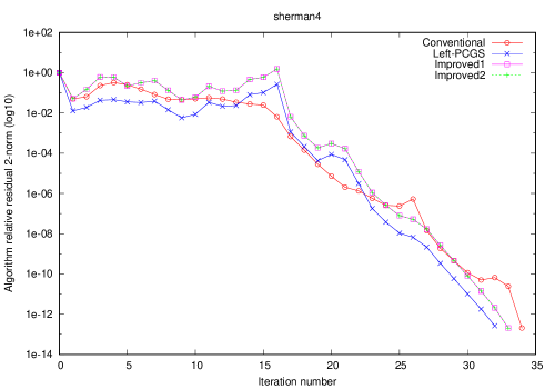
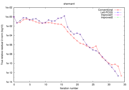
Figure 2: (a) Convergence history of the algorithm relative residual 2-norm for each of the four algorithms (sherman4).

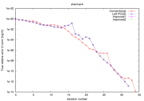
Figure 3: (b) Convergence history of the true relative residual 2-norms for each of the four algorithms (sherman4).

Figure 4: (c) Convergence history of the true relative error 2-norm for each of the four algorithms (sherman4).

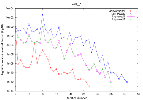
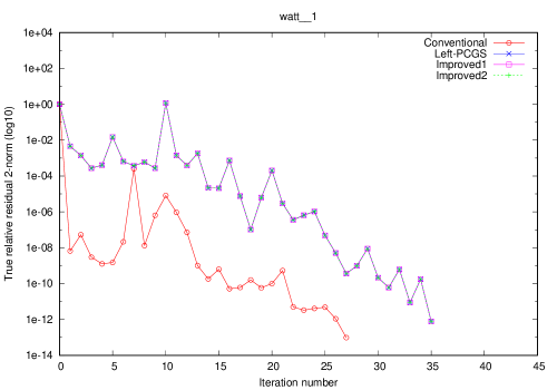
Figure 5: (a) Convergence history of the algorithm relative residual 2-norm for each of the four algorithms (watt 1).

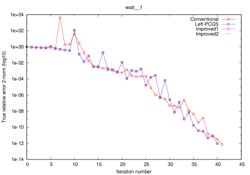
Figure 6: (b) Convergence history of the true relative residual 2-norm for each of the four algorithms (watt 1).

Figure 7: (c) Convergence history of the true relative error 2-norm for each of the four algorithms (watt 1).

From the graphs in Figures 4 to 7, we can see the following: in case (a), Improved1, Improved2, and the left-PCGS show different convergence behaviors, but in cases (b) and (c), they show similar behaviors. These results correspond to the analysis in Section 2.3. Therefore, Algorithms 2.2.1 and 2.2.2 are coordinative to Algorithm 2.1.2 regarding the structures of the solution vector for the polynomial ${\it\Phi}_{k}(\tilde{A})\tilde{\mbox{\boldmath{$r$}}}_{0}$, despite the difference between the residual vectors $\mbox{\boldmath{$r$}}^{+}_{k}$ for the left-PCGS (Algorithm 2.1.2) and $\mbox{\boldmath{$r$}}_{k}$ for Improved1 and Improved2 (Algorithms 2.2.1 and 2.2.2, respectively). The conventional PCGS had a convergence behavior that differs from those of all of the other algorithms for cases (a) to (c).

These numerical results conform to the behavior expected based on the discussion of the relation between the structure of the solution vector and the polynomial. We compared the numerical results with the theoretical results of Sections 2.1.3 and 2.3, and these results are summarized as follows:

1. For case (a), the difference between the residual vector $\mbox{\boldmath{$r$}}^{+}_{k}$ of the left-PCGS and $\mbox{\boldmath{$r$}}_{k}$ has been verified. Accuracy of the left-PCGS is not conclusive, because its high accuracy is caused not by necessity but by accident of its stopping criterion: $\|\mbox{\boldmath{$r$}}^{+}_{k+1}\|_{2}/\|M^{-1}\mbox{\boldmath{$b$}}\|_{2}$.

2. For cases (b) and (c), we verified (2.23):

   $\mbox{\boldmath{$x$}}_{k}=\mbox{\boldmath{$x$}}_{k-1}+{\it\Phi}^{\rm L}_{k-1}(M^{-1}A)\mbox{\boldmath{$r$}}^{+}_{0}\;\;\mapsto\;\;\mbox{\boldmath{$x$}}_{k}=\mbox{\boldmath{$x$}}_{k-1}+M^{-1}{\it\Phi}^{\rm L}_{k-1}(AM^{-1})\mbox{\boldmath{$r$}}_{0}$.

   Furthermore, we verified (2.24): ${\it\Phi}^{\rm R}_{k-1}(AM^{-1})\mbox{\boldmath{$r$}}_{0}\neq{\it\Phi}^{\rm L}_{k-1}(AM^{-1})\mbox{\boldmath{$r$}}_{0}$,

3. The differences between the conventional PCGS, the left-PCGS, Improved1, and Improved2 have been confirmed by examining their convergence behavior. In other word, we considered the relation of the solution vector and the polynomial ${\it\Phi}_{k}(\tilde{A})\tilde{\mbox{\boldmath{$r$}}}_{0}$ between the right system (the conventional PCGS) and the left-PCGS, and between the coordinative PCGSs (Improved1 and Improved2) and the left-PCGS.

4.2 Behavior of the PCGS when it is switched by the ISRV

In this subsection, the experimental environment was the same as that described in Section 4.1, except that we used Matlab 7.8.0 (R2009a), and we gave different ISRVs to the conventional PCGS and Improved1.

We compared five different PCGS algorithms, including using a different ISRV. In the figures, we use the following labels: “Conventional” means the conventional PCGS (Algorithm 2.1.1), for which the ISRV is $\mbox{\boldmath{$r$}}^{\flat}_{0}=\mbox{\boldmath{$r$}}_{0}$; this is a right-preconditioned system. “Impr1-ISRV1” means Improved1 (Algorithm 2.2.1) with ISRV1: $\mbox{\boldmath{$r$}}^{\sharp}_{0}=M^{-1}\mbox{\boldmath{$r$}}_{0}$. “Impr1-ISRV2” means Improved1 with ISRV2: $\mbox{\boldmath{$r$}}^{\sharp}_{0}=M^{\rm T}\mbox{\boldmath{$r$}}_{0}$. “Left” means the left-PCGS (Algorithm 2.1.2), for which the ISRV is $\mbox{\boldmath{$r$}}^{\sharp}_{0}=\mbox{\boldmath{$r$}}^{+}_{0}$. “Conv ISRV9” means the conventional PCGS with ISRV9: $\mbox{\boldmath{$r$}}^{\flat}_{0}=M^{-{\rm T}}M^{-1}\mbox{\boldmath{$r$}}_{0}$.

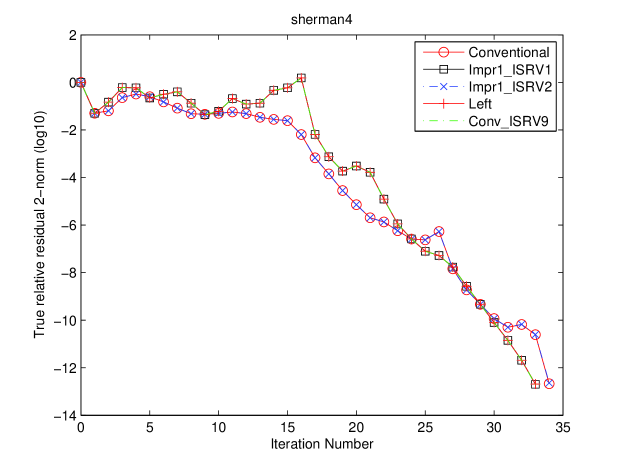
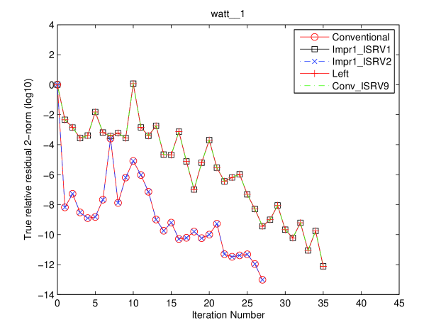
Figure 8: Convergence history of the true relative residual 2-norm of the right- and left-preconditioned PCGS, for each of the five PCGS algorithms with ISRV switching (sherman4).

Figure 9: Convergence history of true relative residual 2-norm of the right- and left-preconditioned PCGS, for each of the five PCGS algorithms with ISRV switching (watt 1).

The convergence histories of “Conventional,” “Impr1-ISRV1,” and “Left” in Figures 9 and 9 are the same as those of “Conventional,” “Improved1,” and “Left-PCGS,” respectively, in Figures 4 and 7.

In both figures, “Impr1-ISRV2” and “Conv ISRV9” were added to verify Theorem 1. The convergence history of “Impr1-ISRV2” is the same as that of “Conventional,” and those of “Impr1-ISRV1” and “Conv ISRV9” are the same as that of “Left.”

We have numerically verified the claims of Section 3; in particular, we have verified Theorem 1.

5 Conclusions

In this paper, an improved PCGS algorithm [7] has been analyzed by mathematically comparing four different PCGS algorithms, and we have focused on the structures of the solution vector and their polynomial ${\it\Phi}_{k}(\tilde{A})\tilde{\mbox{\boldmath{$r$}}}_{0}$. From our analysis and numerical results, we have verified two improved PCGS algorithms. They are both coordinative to the left-preconditioned systems, although their residual vector maintains the basic form $\mbox{\boldmath{$r$}}_{k}$, not $\mbox{\boldmath{$r$}}^{+}_{k}$. For both algorithms, the structures of the solution vector and the polynomial are $\mbox{\boldmath{$x$}}_{k}=\mbox{\boldmath{$x$}}_{k-1}+M^{-1}{\it\Phi}^{\rm L}_{k-1}(AM^{-1})\mbox{\boldmath{$r$}}_{0}$. Furthermore, the numerical results of the improved PCGS with the ILU(0) preconditioner show many advantages, such as effectiveness and consistency across several preconditioners, have also been shown; see [7] and Appendix A. We note that the improved PCGS algorithms share some of the advantages of the conventional PCGS (the right-preconditioned system) and the left-PCGS algorithms, while they avoid some of their disadvantages. Accuracy of the left-PCGS is not controllable, but the Improved1 PCGS algorithm has availability of further improving on accuracy by controlling both residual vectors $\mbox{\boldmath{$r$}}_{k+1}$ and $M^{-1}\mbox{\boldmath{$r$}}_{k+1}\;(\;=\mbox{\boldmath{$r$}}^{+}_{k+1}\;)$ in algorithm. This is our future assignment.

We presented a general definition of the direction of a preconditioned system of linear equations. Furthermore, we have shown that the direction of a preconditioned system for CGS is switched by the construction and setting of the ISRV. This is because the direction of the preconditioning conversion is congruent. We have also shown that the direction of a preconditioned system for CGS is determined by the operations of $\alpha_{k}$ and $\beta_{k}$ and that these intrinsic operations are based on biorthogonality and biconjugacy. However, the structures of these intrinsic operations are the same in all four of the PCGS algorithms. Therefore, we have focused on the ability of the ISRV to switch the direction of a preconditioned system, and such a mechanism may be unique to the bi-Lanczos-type algorithms that are based on the BiCG method; for example, preconditioned BiCGStab, preconditioned GPBiCG and so on. Here, there is an arguable issue on designing their algorithm constructions because such preconditioned bi-Lanczos-type methods have minimal residual operators that have no congruency of preconditioning conversion. This is also our future assignment.

As we analyzed the four PCGS algorithms, we paid particular attention to the vectors. We note that there exist preconditioned BiCG (PBiCG) algorithms that correspond to the preconditioning conversion of each of the PCGS algorithms. The polynomial structure of the PBiCG can be minutely analyzed by replacing the vectors of the PCGS. We have analyzed the four PBiCG algorithms in parallel [8], and each PBiCG corresponds to one of the four PCGS algorithms in this paper. In [8], using the ISRV to switch the direction of a preconditioned system was discussed in detail.

Appendix A Systematic performance evaluation of PCGS

We consider the superficial convergence on three types of preconditioned CGS algorithms; the results shown in Figure 10 provide an overview of this weakness in the left-PCGS. The figure presents a systematic performance evaluation of solving a linear equation by three PCGS algorithms (conventional, left, and improved1) and with nine kinds of preconditioners. Here, we briefly discuss the figure; the details of a systematic performance evaluation can be found in Reference [6], which discusses the right- and the left-preconditioned systems.

The conditions of the numerical experiments presented in this appendix were almost the same as those in Section 4.1 and Reference [6, Section 9.2.2], except for the computational environment. The systematic performance evaluation was executed on a Hitachi HA8000 (AMD Opteron 8356; 2.3 GHz CPU; memory size: 32 GB/node) running the Red Hat Enterprise Linux 5 and the Intel icc 10.1, ifort 10.1 compiler. The maximum number of iterations was equal to the size of each matrix. The test problems were also generated as in Section 4.1 and Reference [6, Section 9.2.2].

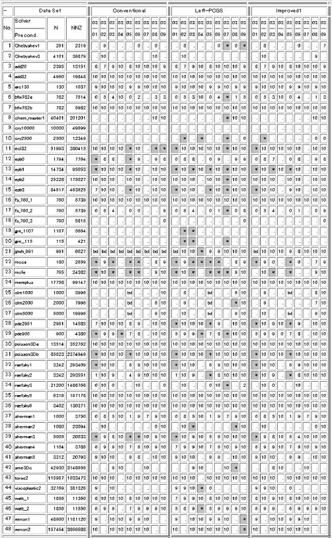
Figure 10: Superficial convergence with three different PCGS methods and nine different preconditioners. Superficial convergence is indicated by an asterisk * with a gray background. Thick lines group columns for (from left to right) the conventional PCGS (Algorithm 2.1.1), the left-PCGS (Algorithm 2.1.2), and Improved1 (Algorithm 2.2.1). Each such frame has a cell for each of the nine preconditioners (from left to right): Point Jacobi [01], ILU(0) [02], SSOR [03], Hybrid type [04], I+S [05], SAINV [06], SA-AMG [07] (with “-saamg unsym true” option), Crout ILU [08], and ILUT [09], where the two digits in [ ] indicate the identification number of the solver or preconditioner. N is the matrix size, and NNZ is the number of nonzero elements.

Figure 10 shows the solution performance data. The rows indicate the forty-eight kinds of linear equations for the coefficient matrix names that are listed in Table 6; the columns indicate the three PCGS algorithms, each of which is subdivided into columns for the nine preconditioners.

Table 6: Real nonsymmetric matrices used for systematic performance evaluation in Figure 10.

Chebyshev{1,3}, add{20,32}, arc130, bfw782{a,b}, chem master1, cry{10000,2500},

ecl32, epb[0-3], fs 760 [1-3], gre {1107,115}, jpwh 991, mcca, mcfe, memplus,

olm{1000, 2000, 5000}, pde{2961,900}, poisson3D{a,b}, raefsky{1,2,3,5,6},

sherman[1-5], sme3Dc, torso2, viscoplastic2, watt {1,2}, xenon{1,2}

The contents of each cell are as follows. The number in each cell indicates the convergence rate. A period (.) indicates that it did not converge until the maximum number of iterations, “bd” indicates that the process broke down, an asterisk ($\ast$) with a gray background indicates that the convergence was superficial convergence, and a blank indicates that it was not solved for some other reason.

Here, we consider the number of cases of superficial convergence. Superficial convergence occurs when the residual vector implies that convergence has occurred, but the solution vector is not a sufficiently accurate approximation to the true residual vector.

The stopping criteria were as follows:

(A.1) $$\|\mbox{\boldmath{$r$}}_{k+1}\|_{2}\;/\;\|\mbox{\boldmath{$b$}}\|_{2}\leq\varepsilon,\;\;\;\;\mbox{(Conventional and Improved1 PCGS)},$$

(A.2) $$\|\mbox{\boldmath{$r$}}^{+}_{k+1}\|_{2}\;/\;\|M^{-1}\mbox{\boldmath{$b$}}\|_{2}\leq\varepsilon,\;\;\;\;\mbox{(Left-PCGS)}.$$

Here, $\mbox{\boldmath{$r$}}_{k+1}$ and $\mbox{\boldmath{$r$}}^{+}_{k+1}$ are the residual vectors for the corresponding PCGS. When these conditions are satisfied, the numerical solution ($\hat{\mbox{\boldmath{$x$}}}_{k+1}$) is obtained, and the true relative residual is calculated as follows:

(A.1) $$\|\mbox{\boldmath{$b$}}-A\hat{\mbox{\boldmath{$x$}}}_{k+1}\|_{2}\;/\;\|\mbox{\boldmath{$b$}}\|_{2}\leq\hat{\varepsilon}.$$

In this systematic performance evaluation, $\varepsilon$ in (2.8') and (2.12') was set to $1.0\times 10^{-12}$. On the other hand, $\hat{\varepsilon}$ in (A.1) was set to $1.0\times 10^{-8}$, because $\hat{\varepsilon}=1.0\times 10^{-12}$ is a stringent value for the tolerance for the true relative residual. We consider that superficial convergence has occurred when (2.8') or (2.12') is satisfied, but (A.1) is not.

Table 7: Number of cases of superficial convergence for each PCGS in Figure 10.

Conventional (Algorithm 2.1.1)	Left-PCGS (Algorithm 2.1.2)	Improved1 (Algorithm 2.2.1)
24	52	18

Figure 10 and Table  7 show that the stopping criterion (2.12') for the left-PCGS is inadequate. Therefore, the left-PCGS has a serious defect, in that superficial convergence can occur; we note that this also occurs with other left-preconditioned algorithms [6].

Just as information on Figure 10, the numbers of problem cases (not converged or not solved, breakdown, and superficial convergence) are 172, 159, and 152 for the conventional PCGS, the left-PCGS, and the improved1 PCGS, respectively.

References

• [1] R. Barrett, et al., Templates for the Solution of Linear Systems: Building Blocks for Iterative Methods, SIAM, Philadelphia, PA, 1994.
• [2] A. M. Bruaset, A Survey of Preconditioned Iterative Methods, Longman Scientific & Technical, Harlow, Essex, UK, 1995.
• [3] T. A. Davis, The University of Florida Sparse Matrix Collection,
http://www.cise.ufl.edu/research/sparse/matrices/
• [4] R. Fletcher, Conjugate gradient methods for indefinite systems, in Numerical Analysis: Proceedings of the Dundee Conference on Numerical Analysis, 1975, G. Watson, ed., Lecture Notes in Math. 506, Springer, New York, pp. 73–89, 1976.
• [5] M. H. Gutknecht, On Lanczos-type methods for Wilson fermions, in Numerical Challenges in Lattice Quantum Chromodynamics, A. Frommer, T. Lippert, B. Medeke, and K. Schilling, eds., Lecture Notes in Computational Science and Engineering 15, Springer, Berlin, pp. 48–65, 2000.
• [6] S. Itoh and M. Sugihara, Systematic performance evaluation of linear solvers using quality control techniques, in Software Automatic Tuning From Concepts to State-of-the-Art Results, K. Naono, K. Teranishi, J. Cavazos, and R. Suda, eds., Springer, New York, pp. 135–152, 2010.
• [7] S. Itoh and M. Sugihara, Formulation of a preconditioned algorithm for the conjugate gradient squared method in accordance with its logical structure, Appl. Math., 6, pp. 1389–1406, 2015.
• [8] S. Itoh and M. Sugihara, The structure of the polynomials in preconditioned BiCG algorithms and the switching direction of preconditioned systems, arXiv:1603.00175 [math.NA], 2016.
• [9] C. Lanczos, Solution of systems of linear equations by minimized iterations, J. Res. Nat. Bur. of Standards, 49, pp. 33–53, 1952.
• [10] Matrix Market, http://math.nist.gov/MatrixMarket/
• [11] G. Meurant, Computer Solution of Large Linear Systems, Elsevier, New York, 2005.
• [12] P. Sonneveld, CGS: A fast Lanczos-type solver for nonsymmetric linear systems, SIAM J. Sci. Stat. Comput., 10, pp. 36–52, 1989.
• [13] SSI project, Lis: Library of iterative solvers for linear systems, http://www.ssisc.org/lis/
• [14] H. A. Van der Vorst, Bi-CGSTAB: A fast and smoothly converging variant of Bi-CG for the solution of nonsymmetric linear systems, SIAM J. Sci. Stat. Comput., 13, pp. 631–644, 1992.
• [15] S.-L. Zhang, GPBi-CG: Generalized product-type methods based on Bi-CG for solving nonsymmetric linear systems, SIAM J. Sci. Comput., 18, pp. 537–551, 1997.