Structure of the polynomials in preconditioned BiCG algorithms and the switching direction of preconditioned systems

Abstract

We present a theorem that defines the direction of a preconditioned system for the bi-conjugate gradient (BiCG) method. The theorem is able to be extended to a variety of preconditioned bi-Lanczos-type methods. We analyze and compare the polynomial structures of four preconditioned BiCG algorithms, in this paper. Finally, we show that the direction of a preconditioned system is switched by construction and by the settings of the initial shadow residual vector.

1 Introduction

The bi-Lanczos-type methods are based on the bi-conjugate gradient (BiCG) method [3, 7] and solve the system of linear equations

(1.1) $$A\mbox{\boldmath{$x$}} = \mbox{\boldmath{$b$}},$$

where $A$ is a large, sparse coefficient matrix of size $n\times n$, $x$ is the solution vector, and $b$ is the right-hand side (RHS) vector. Bi-Lanczos-type methods are a kind of Krylov subspace method, and they assume the existence of a dual system:

(1.2) $$A^{\rm T}\mbox{\boldmath{$x$}}^{\sharp} = \mbox{\boldmath{$b$}}^{\sharp};$$

(1.2) will be referred to as the “shadow system”. In general, the degree $k$ of the Krylov subspace generated by $A$ and $\mbox{\boldmath{$r$}}_{0}$ is displayed as ${\cal K}_{k}\left(A,\mbox{\boldmath{$r$}}_{0}\right)$ $={\rm span}\left\{\mbox{\boldmath{$r$}}_{0},A\mbox{\boldmath{$r$}}_{0},A^{2}\mbox{\boldmath{$r$}}_{0},\cdots,\right.$ $\left.A^{k-1}\mbox{\boldmath{$r$}}_{0}\right\}$, where $\mbox{\boldmath{$r$}}_{0}$ is the initial residual vector $\mbox{\boldmath{$r$}}_{0}=\mbox{\boldmath{$b$}}-A\mbox{\boldmath{$x$}}_{0}$, for an initial guess to the solution $\mbox{\boldmath{$x$}}_{0}$. The Krylov subspace ${\cal K}_{k}\left(A,\mbox{\boldmath{$r$}}_{0}\right)$ generated by the $k$-th iteration forms the structure of $\mbox{\boldmath{$x$}}_{k}\in\mbox{\boldmath{$x$}}_{0}+{\cal K}_{k}\left(A,\mbox{\boldmath{$r$}}_{0}\right)$, where $\mbox{\boldmath{$x$}}_{k}$ is the approximate solution vector (or simply the “solution vector”).

In general, with a preconditioned Krylov subspace method, there are some different algorithms depending on the preconditioning conversion. The structure of the approximate solution is often different for different algorithms, and the performance of a given algorithm may differ substantially from those of other algorithms [5, 6]. In particular, preconditioned bi-Lanczos-type algorithms construct dual systems, and so their analysis is more complex.

The conjugate gradient squared (CGS) method [11] is one of the bi-Lanczos-type methods, and an improved preconditioned CGS (improved PCGS) algorithm has been proposed [5]. In a previous study [6], we compared the structures of the recurrence formula of the solution vectors of four PCGS algorithms, including the improved PCGS. In this paper, we analyze the structures on the polynomials of the preconditioned BiCG (PBiCG) algorithms that correspond to those analyzed in our previous study [6]. Furthermore, in  [6], we also discussed the construction of the initial shadow residual vector (ISRV) in terms of the direction of the preconditioned system; we further analyze this topic in this paper.

In this paper, when we refer to a preconditioned algorithm, we mean one involving a preconditioning operator $M$ or a preconditioning matrix, and by preconditioned system, we mean one that has been converted by some operator(s) based on $M$. These terms never indicate the algorithm for the preconditioning operation itself, such as incomplete LU decomposition or the approximate inverse. For example, for a preconditioned system, the original linear system (1.1) becomes

(1.3) $$\tilde{A}\tilde{\mbox{\boldmath{$x$}}}=\tilde{\mbox{\boldmath{$b$}}},$$

(1.4) $$\tilde{A}=M^{-1}_{L}AM^{-1}_{R},\;\;\tilde{\mbox{\boldmath{$x$}}}=M_{R}\mbox{\boldmath{$x$}},\;\;\tilde{\mbox{\boldmath{$b$}}}=M^{-1}_{L}\mbox{\boldmath{$b$}},$$

with the preconditioner $M=M_{L}M_{R}$ ($M\approx A$). In this paper, the matrix and the vector in the preconditioned system are indicated by a tilde ($\;\tilde{}\;$). However, the conversions in (1.3) and (1.4) are not implemented directly; rather, we construct the preconditioned algorithm that is equivalent to solving (1.3).

This paper is organized as follows. In section 2, we analyze various PBiCG algorithms in terms on their polynomial structures, and we clarify the details of the PCGS algorithms discussed in  [6]. In section 3, we present a theorem that defines the direction of a preconditioned system for the BiCG method. We analyze the mechanism that switches the direction of a preconditioned system for the BiCG method, and we provide the details for some instances that show that, depending on the construction and setting of the ISRV, the BiCG method may be transformed to another method or the direction of the preconditioned system may not be determined. In section 4, we present some numerical results that verify the equivalence of the PBiCG and PCGS methods, the properties of each of the four PBiCG algorithms discussed in section 2, the switching of the direction of a preconditioned system for the BiCG method, and the resulting basic properties, as discussed in section 3. Our conclusions are presented in section 5.

2 Analysis of various preconditioned BiCG algorithms

In this section, we consider four different PBiCG algorithms, these PBiCG algorithms correspond to four PCGS algorithms as shown in Figure 1; these are the same ones discussed in [6].

Algorithm 2 can be used to derive these four PBiCG algorithms.

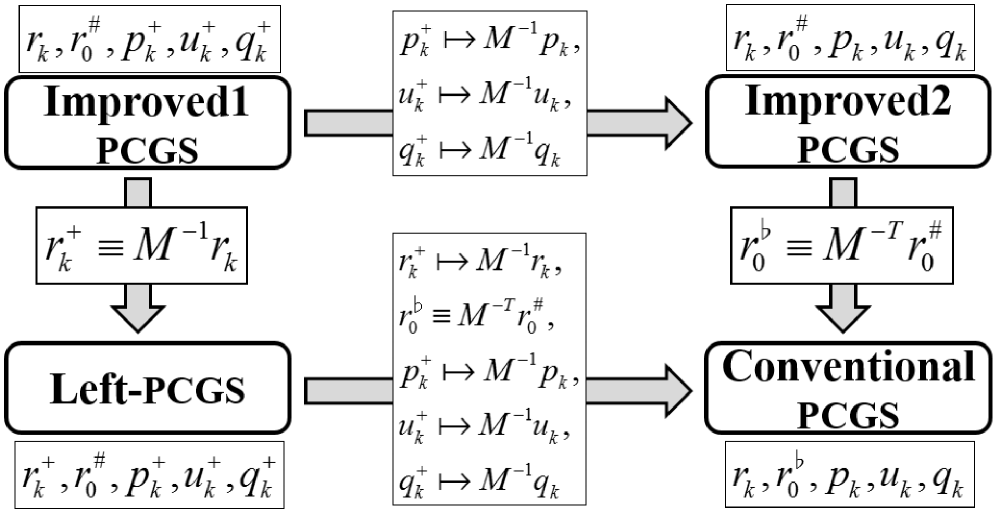
Figure 1: Relations between the four different PCGS algorithms[6]. $\mapsto$ : Splitting left vector to right members (preconditioner and vector), $\equiv$ : Substituting left vector for right members.

Algorithm 1. BiCG method for preconditioned system:

$\tilde{\mbox{\boldmath{$x$}}}_{0}$ is an initial guess, $\;\tilde{\mbox{\boldmath{$r$}}}_{0}=\tilde{\mbox{\boldmath{$b$}}}-\tilde{A}\tilde{\mbox{\boldmath{$x$}}}_{0}$, set $\;\beta^{\rm PBiCG}_{-1}=0$,
$\left(\tilde{\mbox{\boldmath{$r$}}}^{\sharp}_{0},\tilde{\mbox{\boldmath{$r$}}}_{0}\right)\neq 0$, e.g., $\tilde{\mbox{\boldmath{$r$}}}^{\sharp}_{0}=\tilde{\mbox{\boldmath{$r$}}}_{0},\;$
For $k=0,1,2,\cdots,$ until convergence, Do:

$$\tilde{\mbox{\boldmath{$p$}}}_{k}=\tilde{\mbox{\boldmath{$r$}}}_{k}+\beta^{\rm PBiCG}_{k-1}\tilde{\mbox{\boldmath{$p$}}}_{k-1},$$

$$\tilde{\mbox{\boldmath{$p$}}}^{\sharp}_{k}=\tilde{\mbox{\boldmath{$r$}}}^{\sharp}_{k}+\beta^{\rm PBiCG}_{k-1}\tilde{\mbox{\boldmath{$p$}}}^{\sharp}_{k-1},$$

$$\alpha^{\rm PBiCG}_{k}=\frac{\left(\tilde{\mbox{\boldmath{$r$}}}^{\sharp}_{k},\tilde{\mbox{\boldmath{$r$}}}_{k}\right)}{\left(\tilde{\mbox{\boldmath{$p$}}}^{\sharp}_{k},\tilde{A}\tilde{\mbox{\boldmath{$p$}}}_{k}\right)},$$

$$\tilde{\mbox{\boldmath{$x$}}}_{k+1}=\tilde{\mbox{\boldmath{$x$}}}_{k}+\alpha^{\rm PBiCG}_{k}\tilde{\mbox{\boldmath{$p$}}}_{k},$$

$$\tilde{\mbox{\boldmath{$r$}}}_{k+1}=\tilde{\mbox{\boldmath{$r$}}}_{k}-\alpha^{\rm PBiCG}_{k}\tilde{A}\tilde{\mbox{\boldmath{$p$}}}_{k},$$

$$\tilde{\mbox{\boldmath{$r$}}}^{\sharp}_{k+1}=\tilde{\mbox{\boldmath{$r$}}}^{\sharp}_{k}-\alpha^{\rm PBiCG}_{k}\tilde{A}^{\rm T}\tilde{\mbox{\boldmath{$p$}}}^{\sharp}_{k},$$

$$\beta^{\rm PBiCG}_{k}=\frac{\left(\tilde{\mbox{\boldmath{$r$}}}^{\sharp}_{k+1},\tilde{\mbox{\boldmath{$r$}}}_{k+1}\right)}{\left(\tilde{\mbox{\boldmath{$r$}}}^{\sharp}_{k},\tilde{\mbox{\boldmath{$r$}}}_{k}\right)},$$

End Do

Any preconditioned algorithm can be derived by substituting the matrix with the preconditioner for the matrix with the tilde and the vectors with the preconditioner for the vectors with the tilde. Obviously, Algorithm 2 without the preconditioning conversion is the same as the BiCG method. If $\tilde{A}$ is a symmetric positive definite (SPD) matrix and $\tilde{\mbox{\boldmath{$r$}}}^{\sharp}_{0}=\tilde{\mbox{\boldmath{$r$}}}_{0}$, then Algorithm 2 is mathematically equivalent to the conjugate gradient (CG) method [4] for a preconditioned system.

We present the following general definition; however, the PBiCG will also require Theorem 3, which will be presented in section 3.

Definition 1

For the system and solution

(2.1) $$\tilde{A}\tilde{\mbox{\boldmath{$x$}}}=\tilde{\mbox{\boldmath{$b$}}},$$

(2.2) $$\tilde{A}=M^{-1}_{L}AM^{-1}_{R},\;\;\tilde{\mbox{\boldmath{$x$}}}=M_{R}\mbox{\boldmath{$x$}},\;\;\tilde{\mbox{\boldmath{$b$}}}=M^{-1}_{L}\mbox{\boldmath{$b$}},$$

we define the direction of a preconditioned system of linear equations as follows:

• The two-sided preconditioned system: Equation (1.4');

• The right-preconditioned system: $M_{L}=I$ and $M_{R}=M$ in (1.4');

• The left-preconditioned system: $M_{L}=M$ and $M_{R}=I$ in (1.4'),

where $M$ is the preconditioner $M=M_{L}M_{R}$ ($M\approx A$), and $I$ is the identity matrix.

Other vectors in the solving method are not preconditioned. The initial guess is given as $\mbox{\boldmath{$x$}}_{0}$, and $\tilde{\mbox{\boldmath{$x$}}}_{0}=M_{R}\mbox{\boldmath{$x$}}_{0}$.

The recurrence relations of the BiCG for a preconditioned system are

(2.1) $$R_{0}(\tilde{\lambda}) = 1,\;\;P_{0}(\tilde{\lambda})=1,$$

(2.2) $$R_{k}(\tilde{\lambda}) = R_{k-1}(\tilde{\lambda})-\alpha^{\rm PBiCG}_{k-1}\tilde{\lambda}P_{k-1}(\tilde{\lambda}),$$

(2.3) $$P_{k}(\tilde{\lambda}) = R_{k}(\tilde{\lambda})+\beta^{\rm PBiCG}_{k-1}P_{k-1}(\tilde{\lambda}).$$

$R_{k}(\tilde{\lambda})$ is the degree $k$ of the residual polynomial, and $P_{k}(\tilde{\lambda})$ is the degree $k$ of the probing direction polynomial, that is,

(2.4) $$\tilde{\mbox{\boldmath{$r$}}}_{k} = R_{k}(\tilde{A})\tilde{\mbox{\boldmath{$r$}}}_{0},$$

(2.5) $$\tilde{\mbox{\boldmath{$p$}}}_{k} = P_{k}(\tilde{A})\tilde{\mbox{\boldmath{$r$}}}_{0}.$$

Further, to the shadow for the preconditioned system $\tilde{A}^{\rm T}\tilde{\mbox{\boldmath{$x$}}}^{\sharp}=\tilde{\mbox{\boldmath{$b$}}}^{\sharp}$, we have

(2.6) $$\tilde{\mbox{\boldmath{$r$}}}^{\sharp}_{k} = R_{k}(\tilde{A}^{\rm T})\tilde{\mbox{\boldmath{$r$}}}^{\sharp}_{0},$$

(2.7) $$\tilde{\mbox{\boldmath{$p$}}}^{\sharp}_{k} = P_{k}(\tilde{A}^{\rm T})\tilde{\mbox{\boldmath{$r$}}}^{\sharp}_{0}.$$

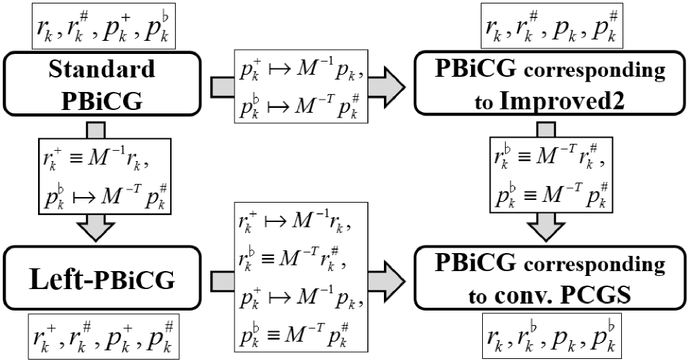
Figure 2: Relations between the four PBiCG algorithms that correspond to the respective PCGS algorithms shown in Figure 1. $\mapsto$ : Splitting left vector to right members (preconditioner and vector), $\equiv$ : Substituting left vector for right members.

Theorem 1 (Lanczos [7], Fletcher [3], Itoh and Sugihara [5])

The BiCG method for a preconditioned system satisfies the following conditions:

(2.8) $$\left(\tilde{\mbox{\boldmath{$r$}}}^{\sharp}_{i},\tilde{\mbox{\boldmath{$r$}}}_{j}\right) = 0\;\;\;(i\neq j),\;\;\;\mbox{ (biorthogonality),}$$

(2.9) $$\left(\tilde{\mbox{\boldmath{$p$}}}^{\sharp}_{i},\tilde{A}\tilde{\mbox{\boldmath{$p$}}}_{j}\right) = 0\;\;\;(i\neq j),\;\;\;\mbox{ (biconjugacy).}$$

Proposition 1

The direction of a preconditioned system is determined by the operations of $\alpha_{k}$ and $\beta_{k}$ in each PBiCG algorithm. These intrinsic operations are based on biorthogonality and biconjugacy.

Theorem 2

There exists a PBiCG algorithm that corresponds to the preconditioning conversion defined by any given PCGS, and the values of $\alpha_{k}$ and $\beta_{k}$ will be equivalent to those of the PCGS.

• See [5]. $\hfill\Box$

  In particular, Reference [5] explains the relations between $\alpha^{\rm PBiCG}_{k}$ and $\beta^{\rm PBiCG}_{k}$ of the standard PBiCG and $\alpha^{\rm PCGS}_{k}$ and $\beta^{\rm PCGS}_{k}$ of the improved PCGS. In this paper, we consider four PBiCG algorithms shown in Figure 2, and these correspond to the four PCGS algorithms shown in Figure 1.

2.1 PBiCG corresponding to conventional PCGS of the right system

The PBiCG algorithm corresponding to the conventional PCGS (the right-preconditioned system) is derived by applying the following preconditioning conversion to Algorithm 2:

(2.10) $$\tilde{A}=M^{-1}_{L}AM^{-1}_{R},\;\tilde{\mbox{\boldmath{$x$}}}_{k}=M_{R}\mbox{\boldmath{$x$}}_{k},\;\tilde{\mbox{\boldmath{$b$}}}=M^{-1}_{L}\mbox{\boldmath{$b$}},\;$$

$$\tilde{\mbox{\boldmath{$r$}}}_{k}=M^{-1}_{L}\mbox{\boldmath{$r$}}_{k},\;\tilde{\mbox{\boldmath{$p$}}}_{k}=M^{-1}_{L}\mbox{\boldmath{$p$}}_{k},\;\tilde{\mbox{\boldmath{$r$}}}^{\sharp}_{k}=M^{\rm T}_{L}\mbox{\boldmath{$r$}}^{\flat}_{k},\;\tilde{\mbox{\boldmath{$p$}}}^{\sharp}_{k}=M^{\rm T}_{L}\mbox{\boldmath{$p$}}^{\flat}_{k}.$$

Algorithm 2.1 is presented below.

Algorithm 2. PBiCG algorithm corresponding to the conventional PCGS:

$\mbox{\boldmath{$x$}}_{0}$ is an initial guess, $\;\mbox{\boldmath{$r$}}_{0}=\mbox{\boldmath{$b$}}-A\mbox{\boldmath{$x$}}_{0},\;\;$ set $\;\beta_{-1}=0$,
$\left(\tilde{\mbox{\boldmath{$r$}}}^{\sharp}_{0},\tilde{\mbox{\boldmath{$r$}}}_{0}\right)=\left(\mbox{\boldmath{$r$}}^{\flat}_{0},\mbox{\boldmath{$r$}}_{0}\right)\neq 0$, e.g., $\mbox{\boldmath{$r$}}^{\flat}_{0}=\mbox{\boldmath{$r$}}_{0},\;$
For $k=0,1,2,\cdots,$ until convergence, Do:

$$\mbox{\boldmath{$p$}}_{k}=\mbox{\boldmath{$r$}}_{k}+\beta_{k-1}\mbox{\boldmath{$p$}}_{k-1},\;\;$$

$$\mbox{\boldmath{$p$}}^{\flat}_{k}=\mbox{\boldmath{$r$}}^{\flat}_{k}+\beta_{k-1}\mbox{\boldmath{$p$}}^{\flat}_{k-1},$$

(2.11) $$\alpha_{k}=\frac{\left(\mbox{\boldmath{$r$}}^{\flat}_{k},\mbox{\boldmath{$r$}}_{k}\right)}{\left(\mbox{\boldmath{$p$}}^{\flat}_{k},AM^{-1}\mbox{\boldmath{$p$}}_{k}\right)},$$

$$\mbox{\boldmath{$x$}}_{k+1}=\mbox{\boldmath{$x$}}_{k}+\alpha_{k}M^{-1}\mbox{\boldmath{$p$}}_{k},$$

$$\mbox{\boldmath{$r$}}_{k+1}=\mbox{\boldmath{$r$}}_{k}-\alpha_{k}AM^{-1}\mbox{\boldmath{$p$}}_{k},\;\;$$

$$\mbox{\boldmath{$r$}}^{\flat}_{k+1}=\mbox{\boldmath{$r$}}^{\flat}_{k}-\alpha_{k}M^{-{\rm T}}A^{\rm T}\mbox{\boldmath{$p$}}^{\flat}_{k},$$

$$\beta_{k}=\frac{\left(\mbox{\boldmath{$r$}}^{\flat}_{k+1},\mbox{\boldmath{$r$}}_{k+1}\right)}{\left(\mbox{\boldmath{$r$}}^{\flat}_{k},\mbox{\boldmath{$r$}}_{k}\right)},$$

End Do

The stopping criterion is

(2.12) $$\frac{\|\mbox{\boldmath{$r$}}_{k+1}\|}{\|\mbox{\boldmath{$b$}}\|}\leq\varepsilon.$$

This algorithm can also be derived by the following conversion:

(2.13) $$\tilde{A}=AM^{-1},\;\tilde{\mbox{\boldmath{$x$}}}_{k}=M\mbox{\boldmath{$x$}}_{k},\;\tilde{\mbox{\boldmath{$b$}}}=\mbox{\boldmath{$b$}},\;$$

$$\tilde{\mbox{\boldmath{$r$}}}_{k}=\mbox{\boldmath{$r$}}_{k},\;\tilde{\mbox{\boldmath{$p$}}}_{k}=\mbox{\boldmath{$p$}}_{k},\;\tilde{\mbox{\boldmath{$r$}}}^{\sharp}_{k}=\mbox{\boldmath{$r$}}^{\flat}_{k},\;\tilde{\mbox{\boldmath{$p$}}}^{\sharp}_{k}=\mbox{\boldmath{$p$}}^{\flat}_{k}.$$

This is the same as using $M_{L}=I$ and $M_{R}=M$ in (2.10). Note that this is the same as preconditioning to obtain $\tilde{A}$, $\tilde{\mbox{\boldmath{$x$}}}_{k}$, and $\tilde{\mbox{\boldmath{$b$}}}$, but not converting the other vectors; thus, it is the right-preconditioned system.

Now, we convert $\tilde{A}$ and $\tilde{\mbox{\boldmath{$r$}}}_{0}$ using (2.10) in order to obtain the polynomial representations of (2.4) and (2.5) as $\tilde{\mbox{\boldmath{$r$}}}_{k}$ and $\tilde{\mbox{\boldmath{$p$}}}_{k}$, respectively:

$$\tilde{\mbox{\boldmath{$r$}}}_{k} = R^{\rm R}_{k}(\tilde{A})\tilde{\mbox{\boldmath{$r$}}}_{0}=M^{-1}_{L}R^{\rm R}_{k}(AM^{-1})\mbox{\boldmath{$r$}}_{0},$$

$$\tilde{\mbox{\boldmath{$p$}}}_{k} = P^{\rm R}_{k}(\tilde{A})\tilde{\mbox{\boldmath{$r$}}}_{0}=M^{-1}_{L}P^{\rm R}_{k}(AM^{-1})\mbox{\boldmath{$r$}}_{0}.$$

We have denoted these polynomials with a superscript “R” , to indicate that Algorithm 2.1, which corresponds to the conventional PCGS method, is a right-preconditioned system [6]. The ISRV is set as $\mbox{\boldmath{$r$}}^{\flat}_{0}=\mbox{\boldmath{$r$}}_{0}$ in this algorithm.

Furthermore, we use (2.10) to convert $\tilde{\mbox{\boldmath{$r$}}}_{k}$ and $\tilde{\mbox{\boldmath{$p$}}}_{k}$:

(2.14) $$\mbox{\boldmath{$r$}}_{k} = R^{\rm R}_{k}(AM^{-1})\mbox{\boldmath{$r$}}_{0},$$

(2.15) $$\mbox{\boldmath{$p$}}_{k} = P^{\rm R}_{k}(AM^{-1})\mbox{\boldmath{$r$}}_{0}.$$

The shadow system is also treated in a similar manner using (2.10):

$$\tilde{\mbox{\boldmath{$r$}}}^{\sharp}_{k} = R^{\rm R}_{k}(\tilde{A}^{\rm T})\tilde{\mbox{\boldmath{$r$}}}^{\sharp}_{0}=M^{\rm T}_{L}R^{\rm R}_{k}(M^{-{\rm T}}A^{\rm T})\mbox{\boldmath{$r$}}^{\flat}_{0},$$

$$\tilde{\mbox{\boldmath{$p$}}}^{\sharp}_{k} = P^{\rm R}_{k}(\tilde{A}^{\rm T})\tilde{\mbox{\boldmath{$r$}}}^{\sharp}_{0}=M^{\rm T}_{L}P^{\rm R}_{k}(M^{-{\rm T}}A^{\rm T})\mbox{\boldmath{$r$}}^{\flat}_{0}.$$

Finally, we have

(2.16) $$\mbox{\boldmath{$r$}}^{\flat}_{k} = R^{\rm R}_{k}(M^{-{\rm T}}A^{\rm T})\mbox{\boldmath{$r$}}^{\flat}_{0},$$

(2.17) $$\mbox{\boldmath{$p$}}^{\flat}_{k} = P^{\rm R}_{k}(M^{-{\rm T}}A^{\rm T})\mbox{\boldmath{$r$}}^{\flat}_{0}.$$

We note that (2.14), (2.15), (2.16), and (2.17) can also be obtained using (2.13).

The structures of biorthogonality (2.8) and biconjugacy (2.9) are as follows:

$$\left(\tilde{\mbox{\boldmath{$r$}}}^{\sharp}_{i},\tilde{\mbox{\boldmath{$r$}}}_{j}\right) = \left(M^{\rm T}_{L}\mbox{\boldmath{$r$}}^{\flat}_{i},M^{-1}_{L}\mbox{\boldmath{$r$}}_{j}\right)=\left(\mbox{\boldmath{$r$}}^{\flat}_{i},\mbox{\boldmath{$r$}}_{j}\right)$$

$$= \left(R^{\rm R}_{i}(M^{-{\rm T}}A^{\rm T})\mbox{\boldmath{$r$}}^{\flat}_{0},\;R^{\rm R}_{j}(AM^{-1})\mbox{\boldmath{$r$}}_{0}\right),$$

$$\left(\tilde{\mbox{\boldmath{$p$}}}^{\sharp}_{i},\tilde{A}\tilde{\mbox{\boldmath{$p$}}}_{j}\right) = \left(M^{\rm T}_{L}\mbox{\boldmath{$p$}}^{\flat}_{i},(M^{-1}_{L}AM^{-1}_{R})(M^{-1}_{L}\mbox{\boldmath{$p$}}_{j})\right)=\left(\mbox{\boldmath{$p$}}^{\flat}_{i},(AM^{-1})\mbox{\boldmath{$p$}}_{j}\right)$$

$$= \left(P^{\rm R}_{i}(M^{-{\rm T}}A^{\rm T})\mbox{\boldmath{$r$}}^{\flat}_{0},\;(AM^{-1})P^{\rm R}_{j}(AM^{-1})\mbox{\boldmath{$r$}}_{0}\right).$$

In Algorithm 2.1, the structures of $\mbox{\boldmath{$r$}}^{\flat}_{k}=R^{\rm R}_{k}(M^{-{\rm T}}A^{\rm T})\mbox{\boldmath{$r$}}^{\flat}_{0}$ and $\mbox{\boldmath{$p$}}^{\flat}_{k}=P^{\rm R}_{k}(M^{-{\rm T}}A^{\rm T})\mbox{\boldmath{$r$}}^{\flat}_{0}$ are fixed, and their coefficient matrices are fixed as $M^{-{\rm T}}A^{\rm T}$, because the ISRV is $\mbox{\boldmath{$r$}}^{\flat}_{0}$, and $R^{\rm R}_{k}(M^{-{\rm T}}A^{\rm T})\mbox{\boldmath{$r$}}^{\flat}_{0}$ cannot be transformed into $M^{-{\rm T}}R^{\rm R}_{k}(A^{\rm T}M^{-{\rm T}})\mbox{\boldmath{$r$}}^{\sharp}_{0}$. Therefore, the coefficient matrix of their linear system is $AM^{-1}$, so $M\mbox{\boldmath{$x$}}_{k+1}=M\mbox{\boldmath{$x$}}_{k}+\alpha^{\rm R}_{k}P^{\rm R}_{k}(AM^{-1})\mbox{\boldmath{$r$}}_{0}$ is structured, where $\alpha^{\rm R}_{k}$ means (2.11); and Algorithm 2.1 is confirmed to correspond to the right-preconditioned system.

2.2 PBiCG corresponding to the left system PCGS (Left-PBiCG)

The left-PBiCG algorithm corresponding to the left-PCGS can be derived by using the following preconditioning conversion in Algorithm 2:

(2.20) $$\tilde{A}=M^{-1}A,\;\tilde{\mbox{\boldmath{$x$}}}_{k}=\mbox{\boldmath{$x$}}_{k},\;\tilde{\mbox{\boldmath{$b$}}}=M^{-1}\mbox{\boldmath{$b$}},\;$$

$$\tilde{\mbox{\boldmath{$r$}}}_{k}=\mbox{\boldmath{$r$}}^{+}_{k},\;\tilde{\mbox{\boldmath{$p$}}}_{k}=\mbox{\boldmath{$p$}}^{+}_{k},\;\tilde{\mbox{\boldmath{$r$}}}^{\sharp}_{k}=\mbox{\boldmath{$r$}}^{\sharp}_{k},\;\tilde{\mbox{\boldmath{$p$}}}^{\sharp}_{k}=\mbox{\boldmath{$p$}}^{\sharp}_{k}.$$

Algorithm 3. PBiCG algorithm corresponding to left-PCGS:

$\mbox{\boldmath{$x$}}_{0}$ is an initial guess, $\;\mbox{\boldmath{$r$}}^{+}_{0}=M^{-1}\left(\mbox{\boldmath{$b$}}-A\mbox{\boldmath{$x$}}_{0}\right),\;\;$ set $\;\beta_{-1}=0$,
$\left(\tilde{\mbox{\boldmath{$r$}}}^{\sharp}_{0},\tilde{\mbox{\boldmath{$r$}}}_{0}\right)=\left(\mbox{\boldmath{$r$}}^{\sharp}_{0},\mbox{\boldmath{$r$}}^{+}_{0}\right)\neq 0$, e.g., $\mbox{\boldmath{$r$}}^{\sharp}_{0}=\mbox{\boldmath{$r$}}^{+}_{0},\;$
For $k=0,1,2,\cdots,$ until convergence, Do:

$$\mbox{\boldmath{$p$}}^{+}_{k}=\mbox{\boldmath{$r$}}^{+}_{k}+\beta_{k-1}\mbox{\boldmath{$p$}}^{+}_{k-1},\;\;$$

$$\mbox{\boldmath{$p$}}^{\sharp}_{k}=\mbox{\boldmath{$r$}}^{\sharp}_{k}+\beta_{k-1}\mbox{\boldmath{$p$}}^{\sharp}_{k-1},$$

(2.21) $$\alpha_{k}=\frac{\left(\mbox{\boldmath{$r$}}^{\sharp}_{k},\mbox{\boldmath{$r$}}^{+}_{k}\right)}{\left(\mbox{\boldmath{$p$}}^{\sharp}_{k},M^{-1}A\mbox{\boldmath{$p$}}^{+}_{k}\right)},$$

$$\mbox{\boldmath{$x$}}_{k+1}=\mbox{\boldmath{$x$}}_{k}+\alpha_{k}\mbox{\boldmath{$p$}}^{+}_{k},$$

$$\mbox{\boldmath{$r$}}^{+}_{k+1}=\mbox{\boldmath{$r$}}^{+}_{k}-\alpha_{k}M^{-1}A\mbox{\boldmath{$p$}}^{+}_{k},\;\;$$

$$\mbox{\boldmath{$r$}}^{\sharp}_{k+1}=\mbox{\boldmath{$r$}}^{\sharp}_{k}-\alpha_{k}A^{\rm T}M^{-{\rm T}}\mbox{\boldmath{$p$}}^{\sharp}_{k},$$

$$\beta_{k}=\frac{\left(\mbox{\boldmath{$r$}}^{\sharp}_{k+1},\mbox{\boldmath{$r$}}^{+}_{k+1}\right)}{\left(\mbox{\boldmath{$r$}}^{\sharp}_{k},\mbox{\boldmath{$r$}}^{+}_{k}\right)},$$

End Do

In this algorithm, the stopping criterion is

(2.22) $$\frac{\|\mbox{\boldmath{$r$}}^{+}_{k+1}\|}{\|M^{-1}\mbox{\boldmath{$b$}}\|}\leq\varepsilon.$$

The polynomials of the linear system are converted as follows:

(2.23) $$\tilde{\mbox{\boldmath{$r$}}}_{k}=R^{\rm L}_{k}(\tilde{A})\tilde{\mbox{\boldmath{$r$}}}_{0}=R^{\rm L}_{k}(M^{-1}A)\mbox{\boldmath{$r$}}^{+}_{0},$$

(2.24) $$\tilde{\mbox{\boldmath{$p$}}}_{k}=P^{\rm L}_{k}(\tilde{A})\tilde{\mbox{\boldmath{$r$}}}_{0}=P^{\rm L}_{k}(M^{-1}A)\mbox{\boldmath{$r$}}^{+}_{0},$$

and

$$\mbox{\boldmath{$r$}}^{+}_{k} = R^{\rm L}_{k}(M^{-1}A)\mbox{\boldmath{$r$}}^{+}_{0},$$

$$\mbox{\boldmath{$p$}}^{+}_{k} = P^{\rm L}_{k}(M^{-1}A)\mbox{\boldmath{$r$}}^{+}_{0}.$$

In the shadow system, we have

$$\tilde{\mbox{\boldmath{$r$}}}^{\sharp}_{k}=R^{\rm L}_{k}(\tilde{A}^{\rm T})\tilde{\mbox{\boldmath{$r$}}}^{\sharp}_{0}=R^{\rm L}_{k}(A^{\rm T}M^{-{\rm T}})\mbox{\boldmath{$r$}}^{\sharp}_{0},$$

$$\tilde{\mbox{\boldmath{$p$}}}^{\sharp}_{k}=P^{\rm L}_{k}(\tilde{A}^{\rm T})\tilde{\mbox{\boldmath{$r$}}}^{\sharp}_{0}=P^{\rm L}_{k}(A^{\rm T}M^{-{\rm T}})\mbox{\boldmath{$r$}}^{\sharp}_{0},$$

and

$$\mbox{\boldmath{$r$}}^{\sharp}_{k} = R^{\rm L}_{k}(A^{\rm T}M^{-{\rm T}})\mbox{\boldmath{$r$}}^{\sharp}_{0},$$

$$\mbox{\boldmath{$p$}}^{\sharp}_{k} = P^{\rm L}_{k}(A^{\rm T}M^{-{\rm T}})\mbox{\boldmath{$r$}}^{\sharp}_{0}.$$

The structures of biorthogonality and biconjugacy are as follows:

$$\left(\tilde{\mbox{\boldmath{$r$}}}^{\sharp}_{i},\tilde{\mbox{\boldmath{$r$}}}_{j}\right) = \left(\mbox{\boldmath{$r$}}^{\sharp}_{i},\mbox{\boldmath{$r$}}^{+}_{j}\right)$$

$$= \left(R^{\rm L}_{i}(A^{\rm T}M^{-{\rm T}})\mbox{\boldmath{$r$}}^{\sharp}_{0},\;R^{\rm L}_{j}(M^{-1}A)\mbox{\boldmath{$r$}}^{+}_{0}\right),$$

$$\left(\tilde{\mbox{\boldmath{$p$}}}^{\sharp}_{i},\tilde{A}\tilde{\mbox{\boldmath{$p$}}}_{j}\right) = \left(\mbox{\boldmath{$p$}}^{\sharp}_{i},(M^{-1}A)\mbox{\boldmath{$p$}}^{+}_{j}\right)$$

$$= \left(P^{\rm L}_{i}(A^{\rm T}M^{-{\rm T}})\mbox{\boldmath{$r$}}^{\sharp}_{0},\;(M^{-1}A)P^{\rm L}_{j}(M^{-1}A)\mbox{\boldmath{$r$}}^{+}_{0}\right).$$

In Algorithm 2.2, the structures of $\mbox{\boldmath{$r$}}^{+}_{k}=R^{\rm L}_{k}(M^{-1}A)\mbox{\boldmath{$r$}}^{+}_{0}$ and $\mbox{\boldmath{$p$}}^{+}_{k}=P^{\rm L}_{k}(M^{-1}A)\mbox{\boldmath{$r$}}^{+}_{0}$ are fixed, and their coefficient matrices are fixed as $M^{-1}A$, because the initial residual vector is $\mbox{\boldmath{$r$}}^{+}_{0}$. Therefore, $\mbox{\boldmath{$x$}}_{k+1}=\mbox{\boldmath{$x$}}_{k}+\alpha^{\rm L}_{k}P^{\rm L}_{k}(M^{-1}A)\mbox{\boldmath{$r$}}^{+}_{0}$ is structured, where $\alpha^{\rm L}_{k}$ means (2.21); and Algorithm 2.2 is confirmed to be the left-preconditioned system. This ISRV is set as $\mbox{\boldmath{$r$}}^{\sharp}_{0}=\mbox{\boldmath{$r$}}^{+}_{0}$.

For reference, this algorithm can also be derived by the following conversion:

(2.27) $$\tilde{A}=M^{-1}_{L}AM^{-1}_{R},\;\tilde{\mbox{\boldmath{$x$}}}_{k}=M_{R}\mbox{\boldmath{$x$}}_{k},\;\tilde{\mbox{\boldmath{$b$}}}=M^{-1}_{L}\mbox{\boldmath{$b$}},\;$$

$$\tilde{\mbox{\boldmath{$r$}}}_{k}=M_{R}\mbox{\boldmath{$r$}}^{+}_{k},\;\tilde{\mbox{\boldmath{$p$}}}_{k}=M_{R}\mbox{\boldmath{$p$}}^{+}_{k},\;\tilde{\mbox{\boldmath{$r$}}}^{\sharp}_{k}=M^{-{\rm T}}_{R}\mbox{\boldmath{$r$}}^{\sharp}_{k},\;\tilde{\mbox{\boldmath{$p$}}}^{\sharp}_{k}=M^{-{\rm T}}_{R}\mbox{\boldmath{$p$}}^{\sharp}_{k}.$$

If $M_{L}=M$ and $M_{R}=I$ are set, then this is the same as (2.20).

2.3 Standard PBiCG

This is the most general algorithm for the PBiCG, and it corresponds to the PCGS algorithm labeled Improved1 in [6]. This algorithm is derived from the following preconditioning conversion applied to Algorithm 2:

(2.28) $$\tilde{A}=M^{-1}_{L}AM^{-1}_{R},\;\tilde{\mbox{\boldmath{$x$}}}_{k}=M_{R}\mbox{\boldmath{$x$}}_{k},\;\tilde{\mbox{\boldmath{$b$}}}=M^{-1}_{L}\mbox{\boldmath{$b$}},\;$$

$$\tilde{\mbox{\boldmath{$r$}}}_{k}=M^{-1}_{L}\mbox{\boldmath{$r$}}_{k},\;\tilde{\mbox{\boldmath{$p$}}}_{k}=M_{R}\mbox{\boldmath{$p$}}^{+}_{k},\;\tilde{\mbox{\boldmath{$r$}}}^{\sharp}_{k}=M^{-{\rm T}}_{R}\mbox{\boldmath{$r$}}^{\sharp}_{k},\;\tilde{\mbox{\boldmath{$p$}}}^{\sharp}_{k}=M^{\rm T}_{L}\mbox{\boldmath{$p$}}^{\flat}_{k}.$$

Algorithm 4. Standard PBiCG algorithm:

$\mbox{\boldmath{$x$}}_{0}$ is an initial guess, $\;\mbox{\boldmath{$r$}}_{0}=\mbox{\boldmath{$b$}}-A\mbox{\boldmath{$x$}}_{0},\;\;$ set $\;\beta_{-1}=0$,
$\left(\tilde{\mbox{\boldmath{$r$}}}^{\sharp}_{0},\tilde{\mbox{\boldmath{$r$}}}_{0}\right)=\left(\mbox{\boldmath{$r$}}^{\sharp}_{0},M^{-1}\mbox{\boldmath{$r$}}_{0}\right)\neq 0$, e.g., $\mbox{\boldmath{$r$}}^{\sharp}_{0}=M^{-1}\mbox{\boldmath{$r$}}_{0},\;$
For $k=0,1,2,\cdots,$ until convergence, Do:

$$\mbox{\boldmath{$p$}}^{+}_{k}=M^{-1}\mbox{\boldmath{$r$}}_{k}+\beta_{k-1}\mbox{\boldmath{$p$}}^{+}_{k-1},\;\;$$

$$\mbox{\boldmath{$p$}}^{\flat}_{k}=M^{-{\rm T}}\mbox{\boldmath{$r$}}^{\sharp}_{k}+\beta_{k-1}\mbox{\boldmath{$p$}}^{\flat}_{k-1},$$

$$\alpha_{k}=\frac{\left(\mbox{\boldmath{$r$}}^{\sharp}_{k},M^{-1}\mbox{\boldmath{$r$}}_{k}\right)}{\left(\mbox{\boldmath{$p$}}^{\flat}_{k},A\mbox{\boldmath{$p$}}^{+}_{k}\right)},$$

$$\mbox{\boldmath{$x$}}_{k+1}=\mbox{\boldmath{$x$}}_{k}+\alpha_{k}\mbox{\boldmath{$p$}}^{+}_{k},$$

$$\mbox{\boldmath{$r$}}_{k+1}=\mbox{\boldmath{$r$}}_{k}-\alpha_{k}A\mbox{\boldmath{$p$}}^{+}_{k},\;\;$$

$$\mbox{\boldmath{$r$}}^{\sharp}_{k+1}=\mbox{\boldmath{$r$}}^{\sharp}_{k}-\alpha_{k}A^{\rm T}\mbox{\boldmath{$p$}}^{\flat}_{k},$$

$$\beta_{k}=\frac{\left(\mbox{\boldmath{$r$}}^{\sharp}_{k+1},M^{-1}\mbox{\boldmath{$r$}}_{k+1}\right)}{\left(\mbox{\boldmath{$r$}}^{\sharp}_{k},M^{-1}\mbox{\boldmath{$r$}}_{k}\right)},$$

End Do

In this algorithm, the stopping criterion is (2.12).

Although sometimes the ISRV is set such that $(\mbox{\boldmath{$r$}}^{\sharp}_{0},\mbox{\boldmath{$r$}}_{0})\neq 0,$ e.g., $\mbox{\boldmath{$r$}}^{\sharp}_{0}=\mbox{\boldmath{$r$}}_{0}$, in many cases, we will assume $(\tilde{\mbox{\boldmath{$r$}}}^{\sharp}_{0},\tilde{\mbox{\boldmath{$r$}}}_{0})\neq 0$, e.g., $\mbox{\boldmath{$r$}}^{\sharp}_{0}=M^{-1}\mbox{\boldmath{$r$}}_{0}$, since $(\tilde{\mbox{\boldmath{$r$}}}^{\sharp}_{0},\tilde{\mbox{\boldmath{$r$}}}_{0})=(M^{-{\rm T}}_{R}\mbox{\boldmath{$r$}}^{\sharp}_{0},M^{-1}_{L}\mbox{\boldmath{$r$}}_{0})=(\mbox{\boldmath{$r$}}^{\sharp}_{0},M^{-1}\mbox{\boldmath{$r$}}_{0})$ from (2.28); see section 3.

The polynomials of the linear system are converted as

(2.29) $$\tilde{\mbox{\boldmath{$r$}}}_{k} = R^{\rm L}_{k}(\tilde{A})\tilde{\mbox{\boldmath{$r$}}}_{0}=M^{-1}_{L}R^{\rm L}_{k}(AM^{-1})\mbox{\boldmath{$r$}}_{0},$$

(2.30) $$\tilde{\mbox{\boldmath{$p$}}}_{k} = P^{\rm L}_{k}(\tilde{A})\tilde{\mbox{\boldmath{$r$}}}_{0}=M^{-1}_{L}P^{\rm L}_{k}(AM^{-1})\mbox{\boldmath{$r$}}_{0},$$

and

(2.31) $$\mbox{\boldmath{$r$}}_{k} = R^{\rm L}_{k}(AM^{-1})\mbox{\boldmath{$r$}}_{0}=MR^{\rm L}_{k}(M^{-1}A)M^{-1}\mbox{\boldmath{$r$}}_{0},$$

(2.32) $$\mbox{\boldmath{$p$}}^{+}_{k} = M^{-1}P^{\rm L}_{k}(AM^{-1})\mbox{\boldmath{$r$}}_{0}=P^{\rm L}_{k}(M^{-1}A)M^{-1}\mbox{\boldmath{$r$}}_{0}.$$

In the shadow system, we have

$$\tilde{\mbox{\boldmath{$r$}}}^{\sharp}_{k} = R^{\rm L}_{k}(\tilde{A}^{\rm T})\tilde{\mbox{\boldmath{$r$}}}^{\sharp}_{0}=M^{-{\rm T}}_{R}R^{\rm L}_{k}(A^{\rm T}M^{-{\rm T}})\mbox{\boldmath{$r$}}^{\sharp}_{0},$$

$$\tilde{\mbox{\boldmath{$p$}}}^{\sharp}_{k} = P^{\rm L}_{k}(\tilde{A}^{\rm T})\tilde{\mbox{\boldmath{$r$}}}^{\sharp}_{0}=M^{-{\rm T}}_{R}P^{\rm L}_{k}(A^{\rm T}M^{-{\rm T}})\mbox{\boldmath{$r$}}^{\sharp}_{0},$$

and

$$\mbox{\boldmath{$r$}}^{\sharp}_{k} = R^{\rm L}_{k}(A^{\rm T}M^{-{\rm T}})\mbox{\boldmath{$r$}}^{\sharp}_{0},$$

$$\mbox{\boldmath{$p$}}^{\flat}_{k} = M^{-{\rm T}}P^{\rm L}_{k}(A^{\rm T}M^{-{\rm T}})\mbox{\boldmath{$r$}}^{\sharp}_{0}.$$

The structures of biorthogonality and biconjugacy are as follows:

$$\left(\tilde{\mbox{\boldmath{$r$}}}^{\sharp}_{i},\tilde{\mbox{\boldmath{$r$}}}_{j}\right) = \left(M^{-{\rm T}}_{R}\mbox{\boldmath{$r$}}^{\sharp}_{i},M^{-1}_{L}\mbox{\boldmath{$r$}}_{j}\right)=\left(M^{-{\rm T}}\mbox{\boldmath{$r$}}^{\sharp}_{i},\mbox{\boldmath{$r$}}_{j}\right)=\left(\mbox{\boldmath{$r$}}^{\sharp}_{i},M^{-1}\mbox{\boldmath{$r$}}_{j}\right)$$

$$= \left(R^{\rm L}_{i}(A^{\rm T}M^{-{\rm T}})\mbox{\boldmath{$r$}}^{\sharp}_{0},\;M^{-1}R^{\rm L}_{j}(AM^{-1})\mbox{\boldmath{$r$}}_{0}\right),$$

$$\left(\tilde{\mbox{\boldmath{$p$}}}^{\sharp}_{i},\tilde{A}\tilde{\mbox{\boldmath{$p$}}}_{j}\right) = \left(M^{\rm T}_{L}\mbox{\boldmath{$p$}}^{\flat}_{i},(M^{-1}_{L}AM^{-1}_{R})(M_{R}\mbox{\boldmath{$p$}}^{+}_{j})\right)=\left(\mbox{\boldmath{$p$}}^{\flat}_{i},A\mbox{\boldmath{$p$}}^{+}_{j}\right)$$

$$= \left(M^{-{\rm T}}P^{\rm L}_{i}(A^{\rm T}M^{-{\rm T}})\mbox{\boldmath{$r$}}^{\sharp}_{0},\;AM^{-1}P^{\rm L}_{j}(AM^{-1})\mbox{\boldmath{$r$}}_{0}\right).$$

Remark 1

In Algorithm 2.3, the biorthogonal and biconjugate structures are not immediately apparent when either $M^{-1}$ operates on the linear system or $M^{-{\rm T}}$ operates on the shadow system. However, Algorithm 2.3 can be reduced to Algorithm 2.2 of the left system by using $\mbox{\boldmath{$r$}}^{+}_{k}\equiv M^{-1}\mbox{\boldmath{$r$}}_{k}$ and $\mbox{\boldmath{$p$}}^{\flat}_{k}\mapsto M^{-{\rm T}}\mbox{\boldmath{$p$}}^{\sharp}_{k}$; therefore, Algorithm 2.3 is coordinative to the left system. The structure of the recurrence formula of the solution vector is $\mbox{\boldmath{$x$}}_{k+1}=\mbox{\boldmath{$x$}}_{k}+\alpha^{\rm L}_{k}P^{\rm L}_{k}(M^{-1}A)\mbox{\boldmath{$r$}}^{+}_{0}\mapsto\mbox{\boldmath{$x$}}_{k+1}=\mbox{\boldmath{$x$}}_{k}+\alpha^{\rm L}_{k}M^{-1}P^{\rm L}_{k}(AM^{-1})\mbox{\boldmath{$r$}}_{0}$; this is obtained by splitting $\mbox{\boldmath{$r$}}^{+}_{0}$. These structures are verified theoretically in section 3 and numerically in section 4.

Remark 2

We explicitly provided the equations for the right endpoints of (2.31) and (2.32). These are the final structures for the setting of $\mbox{\boldmath{$r$}}^{\sharp}_{0}=M^{-1}\mbox{\boldmath{$r$}}_{0}$ (see Example 2 in the Appendix A).

2.4 PBiCG corresponding to Improved2

The PBiCG algorithm corresponding to the Improved2 PCGS algorithm in [6] (Improved2) is derived from applying the following preconditioning conversion to Algorithm 2:

(2.35) $$\tilde{A}=M^{-1}_{L}AM^{-1}_{R},\;\tilde{\mbox{\boldmath{$x$}}}_{k}=M_{R}\mbox{\boldmath{$x$}}_{k},\;\tilde{\mbox{\boldmath{$b$}}}=M^{-1}_{L}\mbox{\boldmath{$b$}},\;$$

$$\tilde{\mbox{\boldmath{$r$}}}_{k}=M^{-1}_{L}\mbox{\boldmath{$r$}}_{k},\;\tilde{\mbox{\boldmath{$p$}}}_{k}=M^{-1}_{L}\mbox{\boldmath{$p$}}_{k},\;\tilde{\mbox{\boldmath{$r$}}}^{\sharp}_{k}=M^{-{\rm T}}_{R}\mbox{\boldmath{$r$}}^{\sharp}_{k},\;\tilde{\mbox{\boldmath{$p$}}}^{\sharp}_{k}=M^{-{\rm T}}_{R}\mbox{\boldmath{$p$}}^{\sharp}_{k}.$$

This is different from the conversion applied to $\tilde{\mbox{\boldmath{$p$}}}_{k}$ and $\tilde{\mbox{\boldmath{$p$}}}^{\sharp}_{k}$ in (2.28) for Algorithm 2.3.

Algorithm 5. PBiCG algorithm corresponding to Improved2:

$\mbox{\boldmath{$x$}}_{0}$ is an initial guess, $\;\mbox{\boldmath{$r$}}_{0}=\mbox{\boldmath{$b$}}-A\mbox{\boldmath{$x$}}_{0},\;\;$ set $\;\beta_{-1}=0$,
$\left(\tilde{\mbox{\boldmath{$r$}}}^{\sharp}_{0},\tilde{\mbox{\boldmath{$r$}}}_{0}\right)=\left(\mbox{\boldmath{$r$}}^{\sharp}_{0},M^{-1}\mbox{\boldmath{$r$}}_{0}\right)\neq 0$, e.g., $\mbox{\boldmath{$r$}}^{\sharp}_{0}=M^{-1}\mbox{\boldmath{$r$}}_{0},\;$
For $k=0,1,2,\cdots,$ until convergence, Do:

(2.36) $$\mbox{\boldmath{$p$}}_{k}=\mbox{\boldmath{$r$}}_{k}+\beta_{k-1}\mbox{\boldmath{$p$}}_{k-1},\;$$

(2.37) $$\left(M^{-1}\mbox{\boldmath{$p$}}_{k}=M^{-1}\mbox{\boldmath{$r$}}_{k}+\beta_{k-1}M^{-1}\mbox{\boldmath{$p$}}_{k-1},\;\right)$$

$$\mbox{\boldmath{$p$}}^{\sharp}_{k}=\mbox{\boldmath{$r$}}^{\sharp}_{k}+\beta_{k-1}\mbox{\boldmath{$p$}}^{\sharp}_{k-1},$$

$$\alpha_{k}=\frac{\left(M^{-{\rm T}}\mbox{\boldmath{$r$}}^{\sharp}_{k},\mbox{\boldmath{$r$}}_{k}\right)}{\left(M^{-{\rm T}}\mbox{\boldmath{$p$}}^{\sharp}_{k},AM^{-1}\mbox{\boldmath{$p$}}_{k}\right)}=\frac{\left(\mbox{\boldmath{$r$}}^{\sharp}_{k},M^{-1}\mbox{\boldmath{$r$}}_{k}\right)}{\left(M^{-{\rm T}}\mbox{\boldmath{$p$}}^{\sharp}_{k},AM^{-1}\mbox{\boldmath{$p$}}_{k}\right)},$$

$$\mbox{\boldmath{$x$}}_{k+1}=\mbox{\boldmath{$x$}}_{k}+\alpha_{k}M^{-1}\mbox{\boldmath{$p$}}_{k},$$

$$\mbox{\boldmath{$r$}}_{k+1}=\mbox{\boldmath{$r$}}_{k}-\alpha_{k}AM^{-1}\mbox{\boldmath{$p$}}_{k},\;\;$$

$$\mbox{\boldmath{$r$}}^{\sharp}_{k+1}=\mbox{\boldmath{$r$}}^{\sharp}_{k}-\alpha_{k}A^{\rm T}M^{-{\rm T}}\mbox{\boldmath{$p$}}^{\sharp}_{k},$$

$$\beta_{k}=\frac{\left(M^{-{\rm T}}\mbox{\boldmath{$r$}}^{\sharp}_{k+1},\mbox{\boldmath{$r$}}_{k+1}\right)}{\left(M^{-{\rm T}}\mbox{\boldmath{$r$}}^{\sharp}_{k},\mbox{\boldmath{$r$}}_{k}\right)}=\frac{\left(\mbox{\boldmath{$r$}}^{\sharp}_{k+1},M^{-1}\mbox{\boldmath{$r$}}_{k+1}\right)}{\left(\mbox{\boldmath{$r$}}^{\sharp}_{k},M^{-1}\mbox{\boldmath{$r$}}_{k}\right)},$$

End Do

In this algorithm , the stopping criterion is (2.12).

The structure of the biorthogonality is the same as that of (2.3) for Algorithm 2.3, because the same preconditioning conversion is used for $\tilde{\mbox{\boldmath{$r$}}}_{k}$ and $\tilde{\mbox{\boldmath{$r$}}}^{\sharp}_{k}$. The probing direction polynomials of the linear and shadow systems are converted as

(2.38) $$\tilde{\mbox{\boldmath{$p$}}}_{k} = P^{\rm L}_{k}(\tilde{A})\tilde{\mbox{\boldmath{$r$}}}_{0}=M^{-1}_{L}P^{\rm L}_{k}(AM^{-1})\mbox{\boldmath{$r$}}_{0},$$

(2.39) $$\tilde{\mbox{\boldmath{$p$}}}^{\sharp}_{k} = P^{\rm L}_{k}(\tilde{A}^{\rm T})\tilde{\mbox{\boldmath{$r$}}}^{\sharp}_{0}=M^{-{\rm T}}_{R}P^{\rm L}_{k}(A^{\rm T}M^{-{\rm T}})\mbox{\boldmath{$r$}}^{\sharp}_{0},$$

and

(2.40) $$\mbox{\boldmath{$p$}}_{k} = P^{\rm L}_{k}(AM^{-1})\mbox{\boldmath{$r$}}_{0}=MP^{\rm L}_{k}(M^{-1}A)M^{-1}\mbox{\boldmath{$r$}}_{0},$$

(2.41) $$\mbox{\boldmath{$p$}}^{\sharp}_{k} = P^{\rm L}_{k}(A^{\rm T}M^{-{\rm T}})\mbox{\boldmath{$r$}}^{\sharp}_{0}.$$

The structure of the biconjugacy is

$$\left(\tilde{\mbox{\boldmath{$p$}}}^{\sharp}_{i},\tilde{A}\tilde{\mbox{\boldmath{$p$}}}_{j}\right) = \left(M^{-{\rm T}}_{R}\mbox{\boldmath{$p$}}^{\sharp}_{i},\;(M^{-1}_{L}AM^{-1}_{R})(M^{-1}_{L}\mbox{\boldmath{$p$}}_{j})\right)=\left(M^{-{\rm T}}\mbox{\boldmath{$p$}}^{\sharp}_{i},\;AM^{-1}\mbox{\boldmath{$p$}}_{j}\right)$$

$$= \left(M^{-{\rm T}}P^{\rm L}_{i}(A^{\rm T}M^{-{\rm T}})\mbox{\boldmath{$r$}}^{\sharp}_{0},\;AM^{-1}P^{\rm L}_{j}(AM^{-1})\mbox{\boldmath{$r$}}_{0}\right).$$

This structure is the same as that of (2.3) for Algorithm 2.3. This ISRV is set as $\mbox{\boldmath{$r$}}^{\sharp}_{0}=M^{-1}\mbox{\boldmath{$r$}}_{0}$.

Remark 3

As before, in Algorithm 2.4, the biorthogonal and biconjugate structures are not immediately apparent when either $M^{-1}$ operates on the linear system or $M^{-{\rm T}}$ operates on the shadow system. However, the structure of the recurrence formula of the solution vector is again $\mbox{\boldmath{$x$}}_{k+1}=\mbox{\boldmath{$x$}}_{k}+\alpha^{\rm L}_{k}M^{-1}P^{\rm L}_{k}(AM^{-1})\mbox{\boldmath{$r$}}_{0}$, because Algorithm 2.4 is equivalent to Algorithm 2.3 on the $\alpha_{k}$ and $\beta_{k}$, the residual and shadow residual vectors, respectively. These properties are verified theoretically in section 3 and numerically in section 4.

Remark 4

We explicitly provided (2.40) for the right endpoint. This is the final structure obtained for $\mbox{\boldmath{$r$}}^{\sharp}_{0}=M^{-1}\mbox{\boldmath{$r$}}_{0}$ (see Remark 2).

2.5 Characteristic features of the four PBiCG algorithms

In this section, we present the characteristics of each of the PBiCG algorithms. These include the construction of the ISRV, the biorthogonal and biconjugate structures of the $\alpha_{k}$ and $\beta_{k}$, and the structures of the recurrence formula of the solution vector. In the following equations, the underlined inner products are the typical descriptions on $\alpha_{k}$ and $\beta_{k}$.

• PBiCG corresponding to the conventional PCGS (Algorithm 2.1):

  $$\mbox{\boldmath{$r$}}^{\flat}_{0} = \mbox{\boldmath{$r$}}_{0},$$

  $$\left(\tilde{\mbox{\boldmath{$r$}}}^{\sharp}_{k},\tilde{\mbox{\boldmath{$r$}}}_{k}\right) = \left(R^{\rm R}_{k}(M^{-{\rm T}}A^{\rm T})\mbox{\boldmath{$r$}}^{\flat}_{0},\;R^{\rm R}_{k}(AM^{-1})\mbox{\boldmath{$r$}}_{0}\right)=\underline{\left(\mbox{\boldmath{$r$}}^{\flat}_{k},\mbox{\boldmath{$r$}}_{k}\right)},$$

  $$\left(\tilde{\mbox{\boldmath{$p$}}}^{\sharp}_{k},\tilde{A}\tilde{\mbox{\boldmath{$p$}}}_{k}\right) = \left(P^{\rm R}_{k}(M^{-{\rm T}}A^{\rm T})\mbox{\boldmath{$r$}}^{\flat}_{0},\;\left(AM^{-1}\right)P^{\rm R}_{k}(AM^{-1})\mbox{\boldmath{$r$}}_{0}\right)$$

  $$= \underline{\left(\mbox{\boldmath{$p$}}^{\flat}_{k},(AM^{-1})\mbox{\boldmath{$p$}}_{k}\right)},$$

  $$M\mbox{\boldmath{$x$}}_{k+1} = M\mbox{\boldmath{$x$}}_{k}+\alpha^{\rm R}_{k}P^{\rm R}_{k}(AM^{-1})\mbox{\boldmath{$r$}}_{0}.$$

• Left-PBiCG (Algorithm 2.2):

  $$\mbox{\boldmath{$r$}}^{\sharp}_{0} = \mbox{\boldmath{$r$}}^{+}_{0},$$

  $$\left(\tilde{\mbox{\boldmath{$r$}}}^{\sharp}_{k},\tilde{\mbox{\boldmath{$r$}}}_{k}\right) = \left(R^{\rm L}_{k}(A^{\rm T}M^{-{\rm T}})\mbox{\boldmath{$r$}}^{\sharp}_{0},\;R^{\rm L}_{k}(M^{-1}A)\mbox{\boldmath{$r$}}^{+}_{0}\right)=\underline{\left(\mbox{\boldmath{$r$}}^{\sharp}_{k},\mbox{\boldmath{$r$}}^{+}_{k}\right)},$$

  $$\left(\tilde{\mbox{\boldmath{$p$}}}^{\sharp}_{k},\tilde{A}\tilde{\mbox{\boldmath{$p$}}}_{k}\right) = \left(P^{\rm L}_{k}(A^{\rm T}M^{-{\rm T}})\mbox{\boldmath{$r$}}^{\sharp}_{0},\;\left(M^{-1}A\right)P^{\rm L}_{k}(M^{-1}A)\mbox{\boldmath{$r$}}^{+}_{0}\right)$$

  $$= \underline{\left(\mbox{\boldmath{$p$}}^{\sharp}_{k},(M^{-1}A)\mbox{\boldmath{$p$}}^{+}_{k}\right)},$$

  $$\mbox{\boldmath{$x$}}_{k+1} = \mbox{\boldmath{$x$}}_{k}+\alpha^{\rm L}_{k}P^{\rm L}_{k}(M^{-1}A)\mbox{\boldmath{$r$}}^{+}_{0}.$$

• Standard PBiCG (Algorithm 2.3):

  $$\mbox{\boldmath{$r$}}^{\sharp}_{0} = M^{-1}\mbox{\boldmath{$r$}}_{0},$$

  $$\left(\tilde{\mbox{\boldmath{$r$}}}^{\sharp}_{k},\tilde{\mbox{\boldmath{$r$}}}_{k}\right) = \left(R^{\rm L}_{k}(A^{\rm T}M^{-{\rm T}})\mbox{\boldmath{$r$}}^{\sharp}_{0},\;M^{-1}R^{\rm L}_{k}(AM^{-1})\mbox{\boldmath{$r$}}_{0}\right)=\underline{\left(\mbox{\boldmath{$r$}}^{\sharp}_{k},M^{-1}\mbox{\boldmath{$r$}}_{k}\right)},$$

  $$\left(\tilde{\mbox{\boldmath{$p$}}}^{\sharp}_{k},\tilde{A}\tilde{\mbox{\boldmath{$p$}}}_{k}\right) = \left(M^{-{\rm T}}P^{\rm L}_{k}(A^{\rm T}M^{-{\rm T}})\mbox{\boldmath{$r$}}^{\sharp}_{0},\;AM^{-1}P^{\rm L}_{k}(AM^{-1})\mbox{\boldmath{$r$}}_{0}\right)$$

  $$= \underline{\left(\mbox{\boldmath{$p$}}^{\flat}_{k},A\mbox{\boldmath{$p$}}^{+}_{k}\right)},$$

  $$\mbox{\boldmath{$x$}}_{k+1} = \mbox{\boldmath{$x$}}_{k}+\alpha^{\rm L}_{k}M^{-1}P^{\rm L}_{k}(AM^{-1})\mbox{\boldmath{$r$}}_{0}.$$

• PBiCG corresponding to Improved2 (Algorithm 2.4):

  $$\mbox{\boldmath{$r$}}^{\sharp}_{0} = M^{-1}\mbox{\boldmath{$r$}}_{0},$$

  $$\left(\tilde{\mbox{\boldmath{$r$}}}^{\sharp}_{k},\tilde{\mbox{\boldmath{$r$}}}_{k}\right) = \left(M^{-{\rm T}}R^{\rm L}_{k}(A^{\rm T}M^{-{\rm T}})\mbox{\boldmath{$r$}}^{\sharp}_{0},\;R^{\rm L}_{k}(AM^{-1})\mbox{\boldmath{$r$}}_{0}\right)$$

  $$= \underline{\left(M^{-{\rm T}}\mbox{\boldmath{$r$}}^{\sharp}_{k},\mbox{\boldmath{$r$}}_{k}\right)}=\left(\mbox{\boldmath{$r$}}^{\sharp}_{k},M^{-1}\mbox{\boldmath{$r$}}_{k}\right),$$

  $$\left(\tilde{\mbox{\boldmath{$p$}}}^{\sharp}_{k},\tilde{A}\tilde{\mbox{\boldmath{$p$}}}_{k}\right) = \left(M^{-{\rm T}}P^{\rm L}_{k}(A^{\rm T}M^{-{\rm T}})\mbox{\boldmath{$r$}}^{\sharp}_{0},\;AM^{-1}P^{\rm L}_{k}(AM^{-1})\mbox{\boldmath{$r$}}_{0}\right)$$

  $$= \underline{\left(M^{-{\rm T}}\mbox{\boldmath{$p$}}^{\sharp}_{k},AM^{-1}\mbox{\boldmath{$p$}}_{k}\right)}=\left(\mbox{\boldmath{$p$}}^{\sharp}_{k},(M^{-1}A)(M^{-1}\mbox{\boldmath{$p$}}_{k})\right),$$

  $$\mbox{\boldmath{$x$}}_{k+1} = \mbox{\boldmath{$x$}}_{k}+\alpha^{\rm L}_{k}M^{-1}P^{\rm L}_{k}(AM^{-1})\mbox{\boldmath{$r$}}_{0}.$$

Although, superficially, it appears that the solution vector has the same recurrence relation in both Algorithm 2.1 and Algorithm 2.4 ($\mbox{\boldmath{$x$}}_{k+1}=\mbox{\boldmath{$x$}}_{k}+\alpha_{k}M^{-1}\mbox{\boldmath{$p$}}_{k}$), they belong to different systems because in Algorithm 2.1, we have $\alpha^{\rm R}_{k}$ and $\mbox{\boldmath{$p$}}_{k}=P^{\rm R}_{k}(AM^{-1})\mbox{\boldmath{$r$}}_{0}\equiv\mbox{\boldmath{$p$}}^{\rm R}_{k}$, whereas in Algorithm 2.4, we have $\alpha^{\rm L}_{k}$ and $\mbox{\boldmath{$p$}}_{k}=P^{\rm L}_{k}(AM^{-1})\mbox{\boldmath{$r$}}_{0}\equiv\mbox{\boldmath{$p$}}^{\rm L}_{k}$.

We have the following proposition about the direction of the preconditioning conversion.

Proposition 2 (Congruency)

There is congruence to a PBiCG algorithm in the direction of the preconditioning conversion.

• We have already shown the following instances: the PBiCG of the right system (Algorithm 2.1) can be derived from the two-sided conversion (2.10); if $M_{L}=I$ and $M_{R}=M$, the conversion of (2.10) is reduced to that of (2.13), then Algorithm 2.1 is derived. Still if $M_{L}=M$, $M_{R}=I$, then Algorithm 2.1 can be derived. Each of the other preconditioned algorithms (Algorithm 2.2, 2.3, and 2.4) has the same relationship to its corresponding preconditioning conversion. $\hfill\Box$

Proposition 3

On the structure of biorthogonality $(\tilde{\mbox{\boldmath{$r$}}}^{\sharp}_{k},\tilde{\mbox{\boldmath{$r$}}}_{k})$ in the iterated part of each PBiCG in the appeared four algorithms, there exists a single preconditioning operator between $\mbox{\boldmath{$r$}}_{k}$ (basic form of the residual vector) and $\mbox{\boldmath{$r$}}^{\sharp}_{k}$ (basic form of the shadow residual vector), such that $M^{-1}$ operates on $\mbox{\boldmath{$r$}}_{k}$ or $M^{-{\rm T}}$ operates on $\mbox{\boldmath{$r$}}^{\sharp}_{k}$.

Here, the basic form of the residual vector of a linear system includes its polynomial structure of $\mbox{\boldmath{$r$}}_{k}=R_{k}(AM^{-1})\mbox{\boldmath{$r$}}_{0}$, and the basic form of the shadow residual vector includes its polynomial structure of $\mbox{\boldmath{$r$}}^{\sharp}_{k}=R_{k}(A^{\rm T}M^{-{\rm T}})\mbox{\boldmath{$r$}}^{\sharp}_{0}$; these vectors and polynomials are not considered when setting the ISRV.

Proof 1) From the viewpoint of the matrix and vector structure of each algorithm:

We split $\mbox{\boldmath{$r$}}^{\flat}_{0}\mapsto M^{-{\rm T}}\mbox{\boldmath{$r$}}^{\sharp}_{0}$ and $\mbox{\boldmath{$r$}}^{+}_{k}\mapsto M^{-1}\mbox{\boldmath{$r$}}_{k}$, in Algorithms 2.1 to 2.4 then we set

$$\left(\tilde{\mbox{\boldmath{$r$}}}^{\sharp}_{k},\tilde{\mbox{\boldmath{$r$}}}_{k}\right) = \underline{\left(\mbox{\boldmath{$r$}}^{\flat}_{k},\;\mbox{\boldmath{$r$}}_{k}\right)}\mapsto\left(M^{-{\rm T}}\mbox{\boldmath{$r$}}^{\sharp}_{k},\;\mbox{\boldmath{$r$}}_{k}\right),$$

$$\left(\tilde{\mbox{\boldmath{$r$}}}^{\sharp}_{k},\tilde{\mbox{\boldmath{$r$}}}_{k}\right) = \underline{\left(\mbox{\boldmath{$r$}}^{\sharp}_{k},\;\mbox{\boldmath{$r$}}^{+}_{k}\right)}\mapsto\left(\mbox{\boldmath{$r$}}^{\sharp}_{k},\;M^{-1}\mbox{\boldmath{$r$}}_{k}\right),$$

$$\left(\tilde{\mbox{\boldmath{$r$}}}^{\sharp}_{k},\tilde{\mbox{\boldmath{$r$}}}_{k}\right) = \underline{\left(\mbox{\boldmath{$r$}}^{\sharp}_{k},\;M^{-1}\mbox{\boldmath{$r$}}_{k}\right)},$$

$$\left(\tilde{\mbox{\boldmath{$r$}}}^{\sharp}_{k},\tilde{\mbox{\boldmath{$r$}}}_{k}\right) = \underline{\left(M^{-{\rm T}}\mbox{\boldmath{$r$}}^{\sharp}_{k},\;\mbox{\boldmath{$r$}}_{k}\right)}=\left(\mbox{\boldmath{$r$}}^{\sharp}_{k},\;M^{-1}\mbox{\boldmath{$r$}}_{k}\right).$$

The underlined inner products are the typical descriptions for the various PBiCG.

In addition, for the two-sided conversion, we obtain

$$\left(\tilde{\mbox{\boldmath{$r$}}}^{\sharp}_{k},\tilde{\mbox{\boldmath{$r$}}}_{k}\right) = \left(M^{-{\rm T}}_{R}\mbox{\boldmath{$r$}}^{\sharp}_{k},\;M^{-1}_{L}\mbox{\boldmath{$r$}}_{k}\right)=\left(M^{-{\rm T}}\mbox{\boldmath{$r$}}^{\sharp}_{k},\;\mbox{\boldmath{$r$}}_{k}\right)=\left(\mbox{\boldmath{$r$}}^{\sharp}_{k},\;M^{-1}\mbox{\boldmath{$r$}}_{k}\right).\qquad\hfill\Box$$

Proof 2) From the viewpoint of the polynomial of the residual vector:

We split $\mbox{\boldmath{$r$}}^{\flat}_{0}\mapsto M^{-{\rm T}}\mbox{\boldmath{$r$}}^{\sharp}_{0}$ and $\mbox{\boldmath{$r$}}^{+}_{k}\mapsto M^{-1}\mbox{\boldmath{$r$}}_{k}$ in Algorithms 2.1 to 2.4, then we set

$$\left(\tilde{\mbox{\boldmath{$r$}}}^{\sharp}_{k},\tilde{\mbox{\boldmath{$r$}}}_{k}\right) = \underline{\left(R_{k}(M^{-{\rm T}}A^{\rm T})\mbox{\boldmath{$r$}}^{\flat}_{0},\;R_{k}(AM^{-1})\mbox{\boldmath{$r$}}_{0}\right)}$$

$$\mapsto \left(M^{-{\rm T}}R_{k}(A^{\rm T}M^{-{\rm T}})\mbox{\boldmath{$r$}}^{\sharp}_{0},\;R_{k}(AM^{-1})\mbox{\boldmath{$r$}}_{0}\right),$$

$$\left(\tilde{\mbox{\boldmath{$r$}}}^{\sharp}_{k},\tilde{\mbox{\boldmath{$r$}}}_{k}\right) = \underline{\left(R_{k}(A^{\rm T}M^{-{\rm T}})\mbox{\boldmath{$r$}}^{\sharp}_{0},\;R_{k}(M^{-1}A)\mbox{\boldmath{$r$}}^{+}_{0}\right)}$$

$$\mapsto \left(R_{k}(A^{\rm T}M^{-{\rm T}})\mbox{\boldmath{$r$}}^{\sharp}_{0},\;M^{-1}R_{k}(AM^{-1})\mbox{\boldmath{$r$}}_{0}\right),$$

$$\left(\tilde{\mbox{\boldmath{$r$}}}^{\sharp}_{k},\tilde{\mbox{\boldmath{$r$}}}_{k}\right) = \underline{\left(R_{k}(A^{\rm T}M^{-{\rm T}})\mbox{\boldmath{$r$}}^{\sharp}_{0},\;M^{-1}R_{k}(AM^{-1})\mbox{\boldmath{$r$}}_{0}\right)},$$

$$\left(\tilde{\mbox{\boldmath{$r$}}}^{\sharp}_{k},\tilde{\mbox{\boldmath{$r$}}}_{k}\right) = \underline{\left(M^{-{\rm T}}R_{k}(A^{\rm T}M^{-{\rm T}})\mbox{\boldmath{$r$}}^{\sharp}_{0},\;R_{k}(AM^{-1})\mbox{\boldmath{$r$}}_{0}\right)}.$$

The underlined inner products are the structures of the polynomial corresponding to the residual vectors in each PBiCG.

In addition, for the two-sided conversion, we obtain

$$\left(\tilde{\mbox{\boldmath{$r$}}}^{\sharp}_{k},\tilde{\mbox{\boldmath{$r$}}}_{k}\right) = \left(R_{k}(M^{-{\rm T}}_{R}A^{\rm T}M^{-{\rm T}}_{L})M^{-{\rm T}}_{R}\mbox{\boldmath{$r$}}^{\sharp}_{0},\;R_{k}(M^{-1}_{L}AM^{-1}_{R})M^{-1}_{L}\mbox{\boldmath{$r$}}_{0}\right)$$

$$= \left(M^{-{\rm T}}_{R}R_{k}(A^{\rm T}M^{-{\rm T}})\mbox{\boldmath{$r$}}^{\sharp}_{0},\;M^{-1}_{L}R_{k}(AM^{-1})\mbox{\boldmath{$r$}}_{0}\right)$$

$$= \left(M^{-{\rm T}}R_{k}(A^{\rm T}M^{-{\rm T}})\mbox{\boldmath{$r$}}^{\sharp}_{0},\;R_{k}(AM^{-1})\mbox{\boldmath{$r$}}_{0}\right)$$

$$= \left(R_{k}(A^{\rm T}M^{-{\rm T}})\mbox{\boldmath{$r$}}^{\sharp}_{0},\;M^{-1}R_{k}(AM^{-1})\mbox{\boldmath{$r$}}_{0}\right).\qquad\hfill\Box$$

Corollary 1

In the biconjugate structure $(\tilde{\mbox{\boldmath{$p$}}}^{\sharp}_{k},\tilde{A}\tilde{\mbox{\boldmath{$p$}}}_{k})$ in the iterated part of each PBiCG algorithm, there exists a single preconditioning operator between $A$ (coefficient matrix) and $\mbox{\boldmath{$p$}}^{\sharp}_{k}$ (basic form of the shadow probing direction vector), such that $M^{-1}$ operates on $A$ or $M^{-{\rm T}}$ operates on $\mbox{\boldmath{$p$}}^{\sharp}_{k}$; furthermore, there exists a single preconditioning operator between $A$ and $\mbox{\boldmath{$p$}}_{k}$ (basic form of the probing direction vector).

Here, the basic form of the probing direction vector of a linear system includes the polynomial structure of $\mbox{\boldmath{$p$}}_{k}=P_{k}(AM^{-1})\mbox{\boldmath{$p$}}_{0}$, and the basic form of the shadow probing direction vector includes the polynomial structure of $\mbox{\boldmath{$p$}}^{\sharp}_{k}=P_{k}(A^{\rm T}M^{-{\rm T}})\mbox{\boldmath{$p$}}^{\sharp}_{0}$. These vectors and polynomials are not considered when setting the ISRV.

3 Switching the direction of the preconditioned system for the BiCG method

From the analyses presented in the previous sections and in [6], we know that the intrinsic biorthogonal and biconjugate structures of the preconditioned system are the same for each of the four PBiCG algorithms and their corresponding PCGS algorithms, and this is independent of the setting of the ISRV. We now consider the other factor that can switch the direction of the preconditioning: the construction and setting of the ISRV.

As stated above, if the coefficient matrix $A$ is SPD and $\mbox{\boldmath{$r$}}^{\sharp}_{0}=\mbox{\boldmath{$r$}}_{0}$, then the BiCG method is mathematically equivalent to the CG method. However, the BiCG method solves systems of linear equations that correspond to a nonsymmetric coefficient matrix, and the ISRV $\mbox{\boldmath{$r$}}^{\sharp}_{0}$ is usually regarded as arbitrary, providing that $(\mbox{\boldmath{$r$}}^{\sharp}_{0},\mbox{\boldmath{$r$}}_{0})\neq 0$. On the other hand, we may construct an arbitrary vector $\mbox{\boldmath{$r$}}^{\sharp}_{0}=U\mbox{\boldmath{$r$}}_{0}$, such that $(\mbox{\boldmath{$r$}}^{\sharp}_{0},U\mbox{\boldmath{$r$}}_{0})\neq 0$. Here, the matrix $U$ is unprescribed. Obviously, $U\mbox{\boldmath{$r$}}_{0}$ can generate random vectors. However, by the appropriate construction of $U$, the BiCG can be reduced to the other method [1, 2]. We show this result as the following proposition.

Proposition 4

If we let $U=A^{\rm T}$ when $\mbox{\boldmath{$r$}}^{\sharp}_{0}=U\mbox{\boldmath{$r$}}_{0}$ in the BiCG method, then we obtain the biconjugate residual (BiCR) method [9, 10] .

Theorem 3

The direction of a preconditioned system for the BiCG method is switched by the construction and setting of the ISRV.

Proof It is sufficient to prove the following cases regarding the biorthogonality. The biconjugacy can be proven in a similar manner.

Case I: If $\left(\tilde{\mbox{\boldmath{$r$}}}^{\sharp}_{0},\tilde{\mbox{\boldmath{$r$}}}_{0}\right)\neq 0$, then $\tilde{\mbox{\boldmath{$r$}}}^{\sharp}_{0}=\tilde{\mbox{\boldmath{$r$}}}_{0}$.

We mention the following special case for future reference.

Case II: If $\left(\tilde{\mbox{\boldmath{$r$}}}^{\sharp}_{0},\tilde{U}\tilde{\mbox{\boldmath{$r$}}}_{0}\right)\neq 0$, then $\tilde{\mbox{\boldmath{$r$}}}^{\sharp}_{0}=\tilde{U}\tilde{\mbox{\boldmath{$r$}}}_{0}$,    ($\tilde{U}$ : preconditioned system of $U$).

I.  The case of $\tilde{U}=I$, such that $\left(\tilde{\mbox{\boldmath{$r$}}}^{\sharp}_{0},\tilde{U}\tilde{\mbox{\boldmath{$r$}}}_{0}\right)=\left(\tilde{\mbox{\boldmath{$r$}}}^{\sharp}_{0},\tilde{\mbox{\boldmath{$r$}}}_{0}\right)\neq 0$ :

With the equation $\tilde{\mbox{\boldmath{$r$}}}^{\sharp}_{0}=\tilde{\mbox{\boldmath{$r$}}}_{0}$, we may construct the following three items. Each item has two verifications, the first one directly applies the ISRV to the polynomials of the preconditioned system, the second applies the ISRV to the polynomials of the standard PBiCG, which have the same form in all items. The double-underlined equations show the construction of the ISRV that is specialized for switching the direction of a preconditioned system; when right-hand side is given (we term “setting”), the direction is fixed.

1. The left-preconditioned system (ISRV1: $\mbox{\boldmath{$r$}}^{\sharp}_{0}=M^{-1}\mbox{\boldmath{$r$}}_{0}$):

   If $\tilde{\mbox{\boldmath{$r$}}}^{\sharp}_{0}=M^{-{\rm T}}_{R}\mbox{\boldmath{$r$}}^{\sharp}_{0},\;\tilde{\mbox{\boldmath{$r$}}}_{0}=M^{-1}_{L}\mbox{\boldmath{$r$}}_{0}$,

   $\left(\tilde{\mbox{\boldmath{$r$}}}^{\sharp}_{0},\tilde{\mbox{\boldmath{$r$}}}_{0}\right)=\left(M^{-{\rm T}}_{R}\mbox{\boldmath{$r$}}^{\sharp}_{0},M^{-1}_{L}\mbox{\boldmath{$r$}}_{0}\right)=\left(\mbox{\boldmath{$r$}}^{\sharp}_{0},M^{-1}\mbox{\boldmath{$r$}}_{0}\right)\neq 0$, then $\mbox{\boldmath{$r$}}^{\sharp}_{0}=M^{-1}\mbox{\boldmath{$r$}}_{0}$.

   This is equivalent to $\tilde{\mbox{\boldmath{$r$}}}^{\sharp}_{0}=\mbox{\boldmath{$r$}}^{\sharp}_{0},\;\tilde{\mbox{\boldmath{$r$}}}_{0}=M^{-1}\mbox{\boldmath{$r$}}_{0}$.

   $\left(\tilde{\mbox{\boldmath{$r$}}}^{\sharp}_{k},\tilde{\mbox{\boldmath{$r$}}}_{k}\right)=\left(R_{k}(\tilde{A}^{\rm T})\tilde{\mbox{\boldmath{$r$}}}^{\sharp}_{0},R_{k}(\tilde{A})\tilde{\mbox{\boldmath{$r$}}}_{0}\right)=\left(R_{k}(A^{\rm T}M^{-{\rm T}})\mbox{\boldmath{$r$}}^{\sharp}_{0},R_{k}(M^{-1}A)(M^{-1}\mbox{\boldmath{$r$}}_{0})\right)$

   $=\left(R^{\rm L}_{k}(A^{\rm T}M^{-{\rm T}})(M^{-1}\mbox{\boldmath{$r$}}_{0}),R^{\rm L}_{k}(M^{-1}A)(M^{-1}\mbox{\boldmath{$r$}}_{0})\right)$.

   In the standard PBiCG with $\mbox{\boldmath{$r$}}^{\sharp}_{0}=M^{-1}\mbox{\boldmath{$r$}}_{0}$ that constructs the left system,

   $\left(\tilde{\mbox{\boldmath{$r$}}}^{\sharp}_{k},\tilde{\mbox{\boldmath{$r$}}}_{k}\right)=\left(R_{k}(A^{\rm T}M^{-{\rm T}})\;\underline{\underline{\mbox{\boldmath{$r$}}^{\sharp}_{0}}},\;M^{-1}R_{k}(AM^{-1})\mbox{\boldmath{$r$}}_{0}\right)$

   $=\left(R^{\rm L}_{k}(A^{\rm T}M^{-{\rm T}})(\underline{\underline{M^{-1}\mbox{\boldmath{$r$}}_{0}}}),R^{\rm L}_{k}(M^{-1}A)(M^{-1}\mbox{\boldmath{$r$}}_{0})\right)$.

2. The right-preconditioned system (ISRV2: $\mbox{\boldmath{$r$}}^{\sharp}_{0}=M^{\rm T}\mbox{\boldmath{$r$}}_{0}$):

   If $\tilde{\mbox{\boldmath{$r$}}}^{\sharp}_{0}=M^{-{\rm T}}_{R}\mbox{\boldmath{$r$}}^{\sharp}_{0},\;\tilde{\mbox{\boldmath{$r$}}}_{0}=M^{-1}_{L}\mbox{\boldmath{$r$}}_{0}$,

   $\left(\tilde{\mbox{\boldmath{$r$}}}^{\sharp}_{0},\tilde{\mbox{\boldmath{$r$}}}_{0}\right)=\left(M^{-{\rm T}}_{R}\mbox{\boldmath{$r$}}^{\sharp}_{0},M^{-1}_{L}\mbox{\boldmath{$r$}}_{0}\right)=\left(M^{-{\rm T}}\mbox{\boldmath{$r$}}^{\sharp}_{0},\mbox{\boldmath{$r$}}_{0}\right)\neq 0$, then $M^{-{\rm T}}\mbox{\boldmath{$r$}}^{\sharp}_{0}\equiv\mbox{\boldmath{$r$}}^{\flat}_{0}=\mbox{\boldmath{$r$}}_{0}$ or $\mbox{\boldmath{$r$}}^{\sharp}_{0}=M^{\rm T}\mbox{\boldmath{$r$}}_{0}$.

   This is equivalent to $\tilde{\mbox{\boldmath{$r$}}}^{\sharp}_{0}=M^{-{\rm T}}\mbox{\boldmath{$r$}}^{\sharp}_{0}\equiv\mbox{\boldmath{$r$}}^{\flat}_{0},\;\tilde{\mbox{\boldmath{$r$}}}_{0}=\mbox{\boldmath{$r$}}_{0}$ .

   $\left(\tilde{\mbox{\boldmath{$r$}}}^{\sharp}_{k},\tilde{\mbox{\boldmath{$r$}}}_{k}\right)=\left(R_{k}(\tilde{A}^{\rm T})\tilde{\mbox{\boldmath{$r$}}}^{\sharp}_{0},R_{k}(\tilde{A})\tilde{\mbox{\boldmath{$r$}}}_{0}\right)=\left(R_{k}(M^{-{\rm T}}A^{\rm T})M^{-{\rm T}}\mbox{\boldmath{$r$}}^{\sharp}_{0},R_{k}(AM^{-1})\mbox{\boldmath{$r$}}_{0}\right)$

   $\equiv\left(R_{k}(M^{-{\rm T}}A^{\rm T})\mbox{\boldmath{$r$}}^{\flat}_{0},R_{k}(AM^{-1})\mbox{\boldmath{$r$}}_{0}\right)$ $=\left(R^{\rm R}_{k}(M^{-{\rm T}}A^{\rm T})\mbox{\boldmath{$r$}}_{0},R^{\rm R}_{k}(AM^{-1})\mbox{\boldmath{$r$}}_{0}\right)$.

   In the standard PBiCG with $\mbox{\boldmath{$r$}}^{\sharp}_{0}=M^{\rm T}\mbox{\boldmath{$r$}}_{0}$ that constructs the right system,

   $\left(\tilde{\mbox{\boldmath{$r$}}}^{\sharp}_{k},\tilde{\mbox{\boldmath{$r$}}}_{k}\right)=\left(R_{k}(A^{\rm T}M^{-{\rm T}})\;\underline{\underline{\mbox{\boldmath{$r$}}^{\sharp}_{0}}},\;M^{-1}R_{k}(AM^{-1})\mbox{\boldmath{$r$}}_{0}\right)$

   $=\left(M^{-{\rm T}}R^{\rm R}_{k}(A^{\rm T}M^{-{\rm T}})(\underline{\underline{M^{\rm T}\mbox{\boldmath{$r$}}_{0}}}),R^{\rm R}_{k}(AM^{-1})\mbox{\boldmath{$r$}}_{0}\right)$

   $=\left(R^{\rm R}_{k}(M^{-{\rm T}}A^{\rm T})\mbox{\boldmath{$r$}}_{0},R^{\rm R}_{k}(AM^{-1})\mbox{\boldmath{$r$}}_{0}\right)$.

3. The two-sided preconditioned system (ISRV3: $\mbox{\boldmath{$r$}}^{\sharp}_{0}=M^{\rm T}_{R}M^{-1}_{L}\mbox{\boldmath{$r$}}_{0}$):

   If $\tilde{\mbox{\boldmath{$r$}}}^{\sharp}_{0}=M^{-{\rm T}}_{R}\mbox{\boldmath{$r$}}^{\sharp}_{0},\;\tilde{\mbox{\boldmath{$r$}}}_{0}=M^{-1}_{L}\mbox{\boldmath{$r$}}_{0}$,

   $\left(\tilde{\mbox{\boldmath{$r$}}}^{\sharp}_{0},\tilde{\mbox{\boldmath{$r$}}}_{0}\right)=\left(M^{-{\rm T}}_{R}\mbox{\boldmath{$r$}}^{\sharp}_{0},M^{-1}_{L}\mbox{\boldmath{$r$}}_{0}\right)\neq 0$, then $M^{-{\rm T}}_{R}\mbox{\boldmath{$r$}}^{\sharp}_{0}=M^{-1}_{L}\mbox{\boldmath{$r$}}_{0}$ or $\mbox{\boldmath{$r$}}^{\sharp}_{0}=M^{\rm T}_{R}M^{-1}_{L}\mbox{\boldmath{$r$}}_{0}$.

   This is obviously equivalent to $\tilde{\mbox{\boldmath{$r$}}}^{\sharp}_{0}=M^{-{\rm T}}_{R}\mbox{\boldmath{$r$}}^{\sharp}_{0},\;\tilde{\mbox{\boldmath{$r$}}}_{0}=M^{-1}_{L}\mbox{\boldmath{$r$}}_{0}$.

   $\left(\tilde{\mbox{\boldmath{$r$}}}^{\sharp}_{k},\tilde{\mbox{\boldmath{$r$}}}_{k}\right)=\left(R_{k}(\tilde{A}^{\rm T})\tilde{\mbox{\boldmath{$r$}}}^{\sharp}_{0},R_{k}(\tilde{A})\tilde{\mbox{\boldmath{$r$}}}_{0}\right)$

   $=\left(R_{k}(M^{-{\rm T}}_{R}A^{\rm T}M^{-{\rm T}}_{L})(M^{-{\rm T}}_{R}\mbox{\boldmath{$r$}}^{\sharp}_{0}),R_{k}(M^{-1}_{L}AM^{-1}_{R})(M^{-1}_{L}\mbox{\boldmath{$r$}}_{0})\right)$

   $=\left(R^{\rm W}_{k}(M^{-{\rm T}}_{R}A^{\rm T}M^{-{\rm T}}_{L})(M^{-1}_{L}\mbox{\boldmath{$r$}}_{0}),R^{\rm W}_{k}(M^{-1}_{L}AM^{-1}_{R})(M^{-1}_{L}\mbox{\boldmath{$r$}}_{0})\right)$.

   In the standard PBiCG with $\mbox{\boldmath{$r$}}^{\sharp}_{0}=M^{\rm T}_{R}M^{-1}_{L}\mbox{\boldmath{$r$}}_{0}$ that constructs the two-sided system,

   $\left(\tilde{\mbox{\boldmath{$r$}}}^{\sharp}_{k},\tilde{\mbox{\boldmath{$r$}}}_{k}\right)=\left(R_{k}(A^{\rm T}M^{-{\rm T}})\;\underline{\underline{\mbox{\boldmath{$r$}}^{\sharp}_{0}}},\;M^{-1}R_{k}(AM^{-1})\mbox{\boldmath{$r$}}_{0}\right)$

   $=\left(R^{\rm W}_{k}(A^{\rm T}M^{-{\rm T}})(\underline{\underline{M^{\rm T}_{R}M^{-1}_{L}\mbox{\boldmath{$r$}}_{0}}}),\;M^{-1}_{R}M^{-1}_{L}R^{\rm W}_{k}(AM^{-1})\mbox{\boldmath{$r$}}_{0}\right)$

   $=\left(M^{\rm T}_{R}R^{\rm W}_{k}(M^{-{\rm T}}_{R}A^{\rm T}M^{-{\rm T}}_{L})(M^{-1}_{L}\mbox{\boldmath{$r$}}_{0}),\;M^{-1}_{R}R^{\rm W}_{k}(M^{-1}_{L}AM^{-1}_{R})(M^{-1}_{L}\mbox{\boldmath{$r$}}_{0})\right)$

   $=\left(R^{\rm W}_{k}(M^{-{\rm T}}_{R}A^{\rm T}M^{-{\rm T}}_{L})(M^{-1}_{L}\mbox{\boldmath{$r$}}_{0}),\;R^{\rm W}_{k}(M^{-1}_{L}AM^{-1}_{R})(M^{-1}_{L}\mbox{\boldmath{$r$}}_{0})\right)$.

II. The case of an arbitrary $\tilde{U}$, such that $\left(\tilde{\mbox{\boldmath{$r$}}}^{\sharp}_{0},\tilde{U}\tilde{\mbox{\boldmath{$r$}}}_{0}\right)\neq 0$ :

• If $\tilde{\mbox{\boldmath{$r$}}}^{\sharp}_{0}=M^{-{\rm T}}_{R}\mbox{\boldmath{$r$}}^{\sharp}_{0},\tilde{\mbox{\boldmath{$r$}}}_{0}=M^{-1}_{L}\mbox{\boldmath{$r$}}_{0}$,

  $\left(\tilde{\mbox{\boldmath{$r$}}}^{\sharp}_{0},\;\tilde{U}\tilde{\mbox{\boldmath{$r$}}}_{0}\right)=\left(M^{-{\rm T}}_{R}\mbox{\boldmath{$r$}}^{\sharp}_{0},\;\tilde{U}M^{-1}_{L}\mbox{\boldmath{$r$}}_{0}\right)\neq 0$,

  then $M^{-{\rm T}}_{R}\mbox{\boldmath{$r$}}^{\sharp}_{0}=\tilde{U}M^{-1}_{L}\mbox{\boldmath{$r$}}_{0}$ or $\mbox{\boldmath{$r$}}^{\sharp}_{0}=M^{\rm T}_{R}\tilde{U}M^{-1}_{L}\mbox{\boldmath{$r$}}_{0}$.

  Here, if $\tilde{U}=I$, then the two-sided system is constructed, because $\underline{\underline{\mbox{\boldmath{$r$}}^{\sharp}_{0}=}}$ $\underline{\underline{M^{\rm T}_{R}M^{-1}_{L}\mbox{\boldmath{$r$}}_{0}}}$ (ISRV3); if $\tilde{U}=M^{-{\rm T}}_{R}M^{-1}_{R}$, then the left system is constructed, because $\underline{\underline{\mbox{\boldmath{$r$}}^{\sharp}_{0}=M^{-1}\mbox{\boldmath{$r$}}_{0}}}$ (ISRV1); and if $\tilde{U}=M^{-{\rm T}}_{R}M^{\rm T}M_{L}=M^{\rm T}_{L}M_{L}$, then the right system is constructed, because $\underline{\underline{\mbox{\boldmath{$r$}}^{\sharp}_{0}=M^{\rm T}\mbox{\boldmath{$r$}}_{0}}}$ (ISRV2).   $\hfill\Box$

In the next section, Theorem 3 will be verified numerically.

Here, we note the following remarks; further information can be found in Appendix A.

Remark 5

For any items for Case I, in the final structure, the coefficient matrix in the residual polynomial is the same as the direction of the preconditioned system; further, the initial residual vector of the linear system is the same as that of the shadow system; that is, $\tilde{\mbox{\boldmath{$r$}}}^{\sharp}_{0}=\tilde{\mbox{\boldmath{$r$}}}_{0}$.

Specifically, in the left system (ISRV1), the final structure is

$$\left(R^{\rm L}_{k}(A^{\rm T}M^{-{\rm T}})(M^{-1}\mbox{\boldmath{$r$}}_{0}),R^{\rm L}_{k}(M^{-1}A)(M^{-1}\mbox{\boldmath{$r$}}_{0})\right);$$

in the right system (ISRV2), the final structure is

$$\left(R^{\rm R}_{k}(M^{-{\rm T}}A^{\rm T})\mbox{\boldmath{$r$}}_{0},R^{\rm R}_{k}(AM^{-1})\mbox{\boldmath{$r$}}_{0}\right);$$

and in the two-sided system (ISRV3), the final structure is

$$\left(R^{\rm W}_{k}(M^{-{\rm T}}_{R}A^{\rm T}M^{-{\rm T}}_{L})(M^{-1}_{L}\mbox{\boldmath{$r$}}_{0}),R^{\rm W}_{k}(M^{-1}_{L}AM^{-1}_{R})(M^{-1}_{L}\mbox{\boldmath{$r$}}_{0})\right).$$

Note that here Proposition 3 is satisfied, and Remark 1 (section  2.3) and Remark 3 (section  2.4) become apparent.

Remark 6

From Proposition 4 and Case II in the proof of Theorem 3, if either $U$ or $\tilde{U}$ is arbitrarily chosen, then the appropriate method for solving and the direction of the preconditioned system may be indeterminable. Even if $\mbox{\boldmath{$r$}}_{0}$ is replaced by an arbitrary vector $s$, then Case II is still proven without loss of generality, because $\mbox{\boldmath{$s$}}=U\mbox{\boldmath{$r$}}_{0}$. Conversely, if $U$ or $\tilde{U}$ is defined adequately, as in Case I for the PBiCG, then the appropriate solving method and the direction of the preconditioned system can be determined.

Remark 7

As mentioned in section 2.3, there are instances in which $(\mbox{\boldmath{$r$}}^{\sharp}_{0},\mbox{\boldmath{$r$}}_{0})$ $\neq 0$ (e.g., $\mbox{\boldmath{$r$}}^{\sharp}_{0}=\mbox{\boldmath{$r$}}_{0}$) at the initial part of the standard PBiCG. However, in this case, $\tilde{A}$ in Algorithm 2 must be SPD, with the modification $(\tilde{\mbox{\boldmath{$r$}}}^{\sharp}_{0},\tilde{\mbox{\boldmath{$r$}}}_{0})\neq 0$ (e.g., $\mbox{\boldmath{$r$}}^{\sharp}_{0}=\mbox{\boldmath{$r$}}_{0}$). The reason for this is as follows. Let $A$ be SPD with the preconditioner $M=CC^{\rm T}$ ($M\approx A$), then the two-sided preconditioning requires $\tilde{A}=C^{-1}AC^{-{\rm T}}$ in order to ensure it is still SPD, and ISRV3 is constructed as $\mbox{\boldmath{$r$}}^{\sharp}_{0}=CC^{-1}\mbox{\boldmath{$r$}}_{0}=\mbox{\boldmath{$r$}}_{0}$.

Remark 8

The definition of the direction of a preconditioned system for the BiCG method requires Theorem 3 in addition to Definition 1.

4 Numerical experiments

In section 4.1, by comparing the value of $\alpha_{k}$ and $\beta_{k}$ for each of the four PBiCG algorithms presented in section 2 and their corresponding PCGS algorithms [6], we verify that the behavior of the right system is different from that of the other preconditioned systems (i.e., the left-preconditioned algorithms and the improved preconditioned algorithms). Next, the switching of the direction of the preconditioned system by the construction and setting of the ISRV (Theorem 3) is verified in section 4.2.

4.1 Behavior of $\alpha_{k}$ and $\beta_{k}$ in the four PBiCG methods and their corresponding PCGS methods

The test problems were generated by using real nonsymmetric matrices obtained from the Matrix Market [8](sherman4 and watt 1). The RHS vector $b$ of (1.1) was generated by setting all elements of the exact solution vector $\mbox{\boldmath{$x$}}_{\rm exact}$ to 1.0. The initial solution was $\mbox{\boldmath{$x$}}_{0}=\mbox{\boldmath{$0$}}$.

The numerical experiments were executed on a Dell Precision T7400 (Intel Xeon E5420, 2.5 GHz CPU, 16 GB RAM) running the Cent OS (kernel 2.6.18) and Matlab 7.8.0 (R2009a).

In all tests, ILU(0) was adopted as the preconditioning operation, and the value “zero” was set to mean the fill-in level. The ISRVs were $\mbox{\boldmath{$r$}}^{\flat}_{0}=\mbox{\boldmath{$r$}}_{0}$ in the PBiCG corresponding to the conventional PCGS (Algorithm 2.1) and the conventional PCGS, they were $\mbox{\boldmath{$r$}}^{\sharp}_{0}=\mbox{\boldmath{$r$}}^{+}_{0}$ in the left-PBiCG (Algorithm 2.2) and the left-PCGS, and they were $\mbox{\boldmath{$r$}}^{\sharp}_{0}=M^{-1}\mbox{\boldmath{$r$}}_{0}$ in the standard PBiCG (Algorithm 2.3), the PBiCG corresponding to Improved2 (Algorithm 2.4), Improved1 (PCGS), and Improved2 (PCGS).

We plotted the values of $\alpha_{k}$ and $\beta_{k}$ for each of the four PBiCG algorithms presented in section 2 and for each of their corresponding PCGS algorithms [6]; these are shown in Figures 6 to 10.

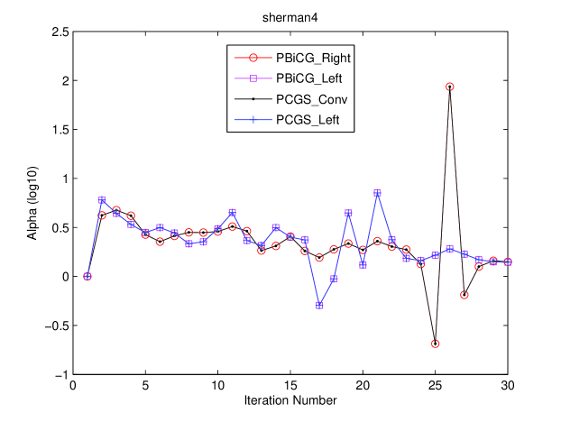
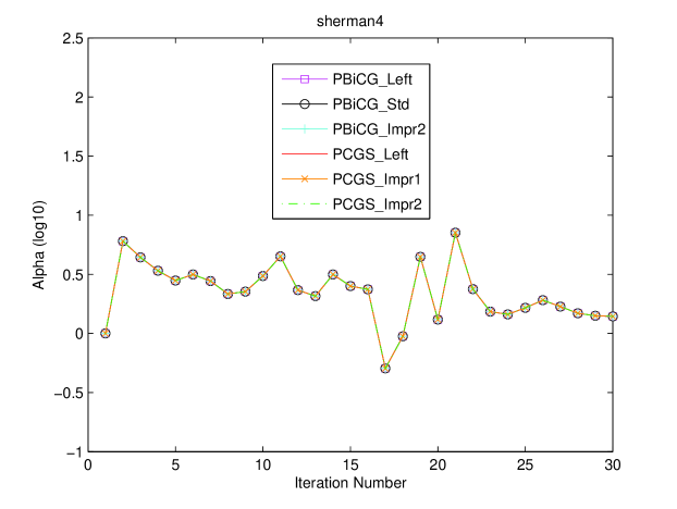
Figure 3: Values of $\alpha_{k}$ for the right- and left-PBiCG, and those of the corresponding PCGS methods (sherman4).

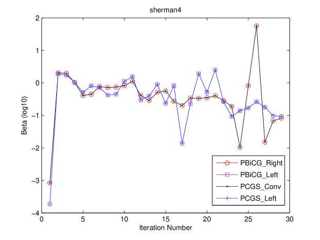
Figure 4: Value of $\alpha_{k}$ for the left- and standard PBiCG and the Improved2 PBiCG, and that of their corresponding PCGS methods (sherman4).

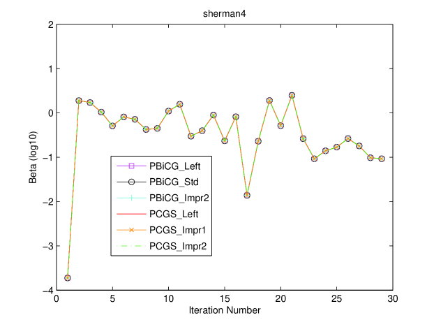
Figure 5: Value of $\beta_{k}$ for the right- and left-PBiCG, and that of the corresponding PCGS method (sherman4).

Figure 6: Value of $\beta_{k}$ for the left- and standard PBiCG and the Improved2 PBiCG, and that of the corresponding PCGS methods (sherman4).

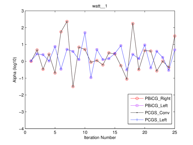
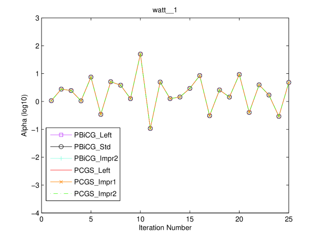
Figure 7: Value of $\alpha_{k}$ for the right- and left-PBiCG, and that of the corresponding PCGS method (watt 1).

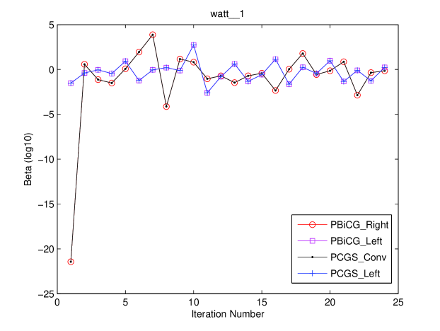
Figure 8: Value of $\alpha_{k}$ for the left- and standard PBiCG and the Improved2 PBiCG, and that of the corresponding PCGS method (watt 1).

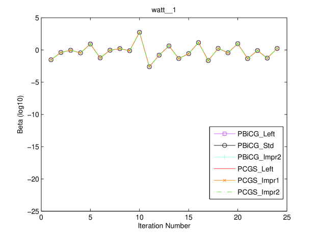
Figure 9: Value of $\beta_{k}$ for the right- and left-PBiCG, and that of the corresponding PCGS method (watt 1).

Figure 10: Value of $\beta_{k}$ for the left- and standard PBiCG and the Improved2 PBiCG, and that of the corresponding PCGS method (watt 1).

The labels in the graphs are as follows:

PBiCG Right (Algorithm 2.1) means the PBiCG corresponding to the conventional PCGS, that is, the right-preconditioned system.

PBiCG Left (Algorithm 2.2) means the PBiCG of the left-preconditioned system.

PBiCG Std (Algorithm 2.3) means the PBiCG of the standard preconditioned BiCG, that is, the PBiCG corresponding to Improved1.

PBiCG Impr2 (Algorithm 2.4) means the PBiCG corresponding to the Improved2 PCGS.

PCGS Conv means the PCGS of the conventional preconditioning conversion.

PCGS Left means the PCGS of the left-preconditioned system.

PCGS Impr1 means the PCGS of Improved1.

PCGS Impr2 means the PCGS of Improved2.

Figures  6 and 10 show the behavior of $\alpha_{k}$ for the right-PBiCG and the left-PBiCG and their corresponding PCGS algorithms. Figures 6 and 10 show the behavior of $\alpha_{k}$ for the left-PBiCG, the standard PBiCG, the Improved2 PBiCG (the PBiCG corresponding to the Improved2 PCGS), and the corresponding PCGS algorithms. From these results, we know that for each of the four PBiCGs, the value of $\alpha_{k}$ is the same as that in their respective PCGS, but the values for the right-PBiCG and for the conventional PCGS are different from the others. A comparison of these results on $\beta_{k}$ can be seen in Figures 6, 6, 10, and 10.

In these graphs, the behaviors of $\alpha_{k}$ and $\beta_{k}$ are the same for each PBiCG algorithm and its corresponding PCGS algorithm; that is, we numerically verified the correspondence between the PBiCG algorithms in Figure 2 in section 2 and the PCGS algorithms in Figure 1 (also see [6]). We also verified that the standard PBiCG (Algorithm 2.3) is coordinative to the left-PBiCG (Algorithm 2.2); that is, $\alpha_{k}$ and $\beta_{k}$ are equivalent, although the residual vector is not ($\mbox{\boldmath{$r$}}^{+}_{k}\equiv M^{-1}\mbox{\boldmath{$r$}}_{k}$, where $\mbox{\boldmath{$r$}}_{k}$ is the standard PBiCG, and $\mbox{\boldmath{$r$}}^{+}_{k}$ is the left-PBiCG). We also verified the difference between the right-preconditioned system and the left-preconditioned system, including the standard PBiCG, because the behavior of $\alpha_{k}$ and $\beta_{k}$ in the conventional PCGS and its corresponding PBiCG are different from the behaviors seen in the other algorithms.

4.2 Behavior of the left-, right-, and two-sided PBiCG and standard PBiCG when switched by the ISRV

For the experiments described in this subsection, the experimental environment was the same as that described in section 4.1, but the ISRVs of the PBiCG method were different.

We will verify Theorem 3 by using the BiCG for the preconditioned system (Algorithm 2) and the standard PBiCG (Algorithm 2.3) with three different ISRVs. Here, Algorithm 2 is based on Definition 1, and Algorithm 2 is used to construct the left-preconditioned system with $M_{L}=M$ and $M_{R}=I$ (PrecDirl-BiCG); it is used to construct the right-preconditioned system with $M_{L}=I$ and $M_{R}=M$ (PrecDirr-BiCG); and it is used to construct the two-sided preconditioned system (PrecDirw-BiCG), for the above algorithms; the ISRV was uniformly set to $\tilde{\mbox{\boldmath{$r$}}}^{\sharp}_{0}=\tilde{\mbox{\boldmath{$r$}}}_{0}$. The algorithm relative residual 2-norm was adjusted as following: $\|M\tilde{\mbox{\boldmath{$r$}}}_{k+1}\|_{2}/\|\mbox{\boldmath{$b$}}\|_{2}$ for the left system, $\|\tilde{\mbox{\boldmath{$r$}}}_{k+1}\|_{2}/\|\mbox{\boldmath{$b$}}\|_{2}$ for the right system, and $\|M_{L}\tilde{\mbox{\boldmath{$r$}}}_{k+1}\|_{2}/\|\mbox{\boldmath{$b$}}\|_{2}$ for the two-sided system. On the other hand, as shown in Theorem 3, Algorithm 2.3 was used to construct the left-preconditioned system with $\mbox{\boldmath{$r$}}^{\sharp}_{0}=M^{-1}\mbox{\boldmath{$r$}}_{0}$ (ISRV1-PBiCG), the right-preconditioned system with $\mbox{\boldmath{$r$}}^{\sharp}_{0}=M^{\rm T}\mbox{\boldmath{$r$}}_{0}$ (ISRV2-PBiCG), and the two-sided preconditioned system with $\mbox{\boldmath{$r$}}^{\sharp}_{0}=M^{\rm T}_{R}M^{-1}_{L}\mbox{\boldmath{$r$}}_{0}$ (ISRV3-PBiCG), these algorithm relative residual 2-norm were all $\|\mbox{\boldmath{$r$}}_{k+1}\|_{2}/\|\mbox{\boldmath{$b$}}\|_{2}$ .

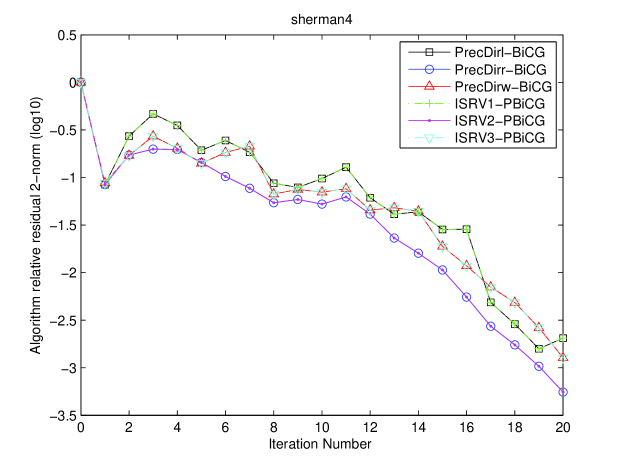
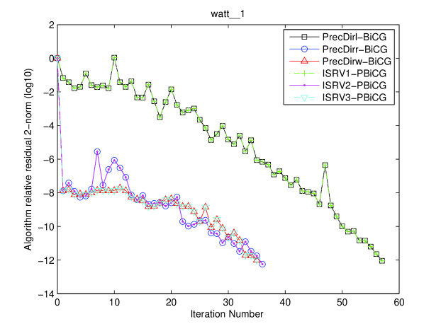
Figure 11: Behavior of the algorithm relative residual 2-norm for the left-, right-, and two-sided PBiCG and the standard PBiCG, with three different settings for the ISRV (sherman4).

Figure 12: Behavior of the algorithm relative residual 2-norm for the left-, right-, and two-sided PBiCG and the standard PBiCG, with three different settings for the ISRV (watt 1).

Figures 12 and 12 illustrate the equivalence of the direction of a preconditioned system obtained by Algorithm 2 based on Definition 1 and the direction switching due to the ISRV when using Algorithm 2.3; this occurs because the left-preconditioned system (PrecDirl-BiCG) has the same behavior as that of the standard PBiCG with ISRV1, the right-preconditioned system (PrecDirr-BiCG) has the same behavior as that of the standard PBiCG with ISRV2, and the two-sided preconditioned system (PrecDirw-BiCG) has the same behavior as that of the standard PBiCG with ISRV3.

5 Conclusions

In this paper, we analyzed four different preconditioned BiCG (PBiCG) algorithms, from the viewpoint of their polynomial structure. These PBiCG algorithms correspond to the four PCGS algorithms considered in [6].

We have shown the mechanism that determines the direction of such a preconditioned system; that is, the direction is determined by $\alpha_{k}$ and $\beta_{k}$, which are constructed by biorthogonal and biconjugate operations. However, the biorthogonal and biconjugate structures of the polynomials of the four PBiCG methods are all the same. Therefore, we have identified that the final factor that can switch the direction of such a preconditioned system is the construction and setting of the ISRV. In particular, we have shown that the direction of the preconditioned system has never been fixed without using the relation $\tilde{\mbox{\boldmath{$r$}}}^{\sharp}_{0}=\tilde{\mbox{\boldmath{$r$}}}_{0}$. Furthermore, we have shown an additional theorem regarding the definition of the direction of a preconditioned system for a BiCG method for solving linear equations. In other words, the construction and setting of the ISRV affect not only the shadow system, but also the linear system on the direction of the preconditioned system, due to the inner product of $\alpha_{k}$ and $\beta_{k}$.

These properties of PBiCG methods are commonly discussed in the literature of preconditioned bi-Lanczos-type algorithms, for example, preconditioned CGS (PCGS) and preconditioned BiCG stabilized (PBiCGStab) algorithms [12], and so on. Further, Theorem 3 presented by this paper is able to be extended to a variety of preconditioned bi-Lanczos-type algorithms. On the other hand, PCGS algorithms are congruent to the direction of the preconditioning conversion, and this has already been analyzed [6]; though, PBiCGStab algorithms are not congruent, and they will be analyzed as an area of future work.

Appendix A Stepwise analysis of the polynomials of the standard PBiCG

Here we present detailed examples of the polynomials of the standard PBiCG (Algorithm 2.3) when using ISRV3 ($\mbox{\boldmath{$r$}}^{\sharp}_{0}=M^{\rm T}_{R}M^{-1}_{L}\mbox{\boldmath{$r$}}_{0}$, Example 1) and the ISRV1 ($\mbox{\boldmath{$r$}}^{\sharp}_{0}=M^{-1}\mbox{\boldmath{$r$}}_{0}$, Example 2); we perform a stepwise analysis by using the recurrence relations (2.1) to (2.3) in section 2.

We will use the following notation: $\tilde{A}_{w}$ ( $=M^{-1}_{L}AM^{-1}_{R}$) means the two-sided preconditioning conversion, $\tilde{A}_{l}$ ( $=M^{-1}A$) means the left preconditioning conversion, and $\tilde{A}_{r}$ ( $=AM^{-1}$) means the right preconditioning conversion.

The initial values of the polynomials in the preconditioned system are as follows:

(A.1) $$P_{0}(\tilde{A}_{w})=P_{0}(\tilde{A}_{l})=P_{0}(\tilde{A}_{r})=I,$$

(A.2) $$R_{0}(\tilde{A}_{w})=R_{0}(\tilde{A}_{l})=R_{0}(\tilde{A}_{r})=I.$$

Example 1. Details of standard PBiCG algorithm with ISRV3:

$\mbox{\boldmath{$x$}}_{0}$ is an initial guess, $\;\mbox{\boldmath{$r$}}_{0}=\mbox{\boldmath{$b$}}-A\mbox{\boldmath{$x$}}_{0},\;\;$ set $\;\beta_{-1}=0$,
$\left(\tilde{\mbox{\boldmath{$r$}}}^{\sharp}_{0},\tilde{\mbox{\boldmath{$r$}}}_{0}\right)=\left(M^{-{\rm T}}_{R}\mbox{\boldmath{$r$}}^{\sharp}_{0},M^{-1}_{L}\mbox{\boldmath{$r$}}_{0}\right)\neq 0$, e.g., $\mbox{\boldmath{$r$}}^{\sharp}_{0}=M_{R}^{\rm T}M^{-1}_{L}\mbox{\boldmath{$r$}}_{0}$,

$$k=0\;:$$

(A.3) $$\mbox{\boldmath{$p$}}^{+}_{0} = M^{-1}\mbox{\boldmath{$r$}}_{0}=M^{-1}_{R}M^{-1}_{L}\mbox{\boldmath{$r$}}_{0},$$

(A.4) $$\mbox{\boldmath{$p$}}^{\flat}_{0} = M^{-{\rm T}}\mbox{\boldmath{$r$}}^{\sharp}_{0}=M^{-{\rm T}}(M_{R}^{\rm T}M^{-1}_{L})\mbox{\boldmath{$r$}}_{0}=M^{-{\rm T}}_{L}M^{-1}_{L}\mbox{\boldmath{$r$}}_{0},$$

$$\alpha_{0} = \frac{\left(\mbox{\boldmath{$r$}}^{\sharp}_{0},M^{-1}\mbox{\boldmath{$r$}}_{0}\right)}{\left(\mbox{\boldmath{$p$}}^{\flat}_{0},A\mbox{\boldmath{$p$}}^{+}_{0}\right)}=\frac{\left((M_{R}^{\rm T}M^{-1}_{L})\mbox{\boldmath{$r$}}_{0},M^{-1}\mbox{\boldmath{$r$}}_{0}\right)}{\left(M^{-{\rm T}}_{L}M^{-1}_{L}\mbox{\boldmath{$r$}}_{0},A(M^{-1}\mbox{\boldmath{$r$}}_{0})\right)}$$

$$= \frac{\left(M^{-1}_{L}\mbox{\boldmath{$r$}}_{0},M^{-1}_{L}\mbox{\boldmath{$r$}}_{0}\right)}{\left(M^{-1}_{L}\mbox{\boldmath{$r$}}_{0},(M^{-1}_{L}AM^{-1}_{R})M^{-1}_{L}\mbox{\boldmath{$r$}}_{0}\right)}\equiv\alpha^{\rm W}_{0},$$

(A.6) $$\mbox{\boldmath{$x$}}_{1} = \mbox{\boldmath{$x$}}_{0}+\alpha^{\rm W}_{0}\mbox{\boldmath{$p$}}^{+}_{0}=\mbox{\boldmath{$x$}}_{0}+\alpha^{\rm W}_{0}M^{-1}\mbox{\boldmath{$r$}}_{0}=\mbox{\boldmath{$x$}}_{0}+\alpha^{\rm W}_{0}M^{-1}_{R}M^{-1}_{L}\mbox{\boldmath{$r$}}_{0},$$

(A.7) $$\mbox{\boldmath{$r$}}_{1} = \mbox{\boldmath{$r$}}_{0}-\alpha^{\rm W}_{0}A\mbox{\boldmath{$p$}}^{+}_{0}$$

$$= M_{L}(I-\alpha^{\rm W}_{0}(M^{-1}_{L}AM^{-1}_{R}))M^{-1}_{L}\mbox{\boldmath{$r$}}_{0}\;\;\;\;\;\;\;\;\;\;\;\;\;=\underline{\underline{M_{L}R^{\rm W}_{1}(\tilde{A}_{w})M^{-1}_{L}\mbox{\boldmath{$r$}}_{0}}}$$

(A.8) $$= M(I-\alpha^{\rm W}_{0}(M^{-1}A))M^{-1}\mbox{\boldmath{$r$}}_{0}\;\;\;\;\;\;\;\;\;\;\;\;\;\;\;\;\;\;\;\;\;\;\;=\underline{\underline{MR^{\rm W}_{1}(\tilde{A}_{l})M^{-1}\mbox{\boldmath{$r$}}_{0}}}$$

(A.9) $$= \mbox{\boldmath{$r$}}_{0}-\alpha^{\rm W}_{0}AM^{-1}\mbox{\boldmath{$r$}}_{0}=(I-\alpha^{\rm W}_{0}(AM^{-1}))\mbox{\boldmath{$r$}}_{0}\;\;\;=\underline{\underline{R^{\rm W}_{1}(\tilde{A}_{r})\mbox{\boldmath{$r$}}_{0}}},$$

$$\mbox{\boldmath{$r$}}^{\sharp}_{1} = \mbox{\boldmath{$r$}}^{\sharp}_{0}-\alpha^{\rm W}_{0}A^{\rm T}\mbox{\boldmath{$p$}}^{\flat}_{0}=(M_{R}^{\rm T}M^{-1}_{L})\mbox{\boldmath{$r$}}_{0}-\alpha^{\rm W}_{0}A^{\rm T}(M^{-{\rm T}}_{L}M^{-1}_{L}\mbox{\boldmath{$r$}}_{0})$$

$$= M_{R}^{\rm T}(I-\alpha^{\rm W}_{0}(M^{-{\rm T}}_{R}A^{\rm T}M^{-{\rm T}}_{L}))M^{-1}_{L}\mbox{\boldmath{$r$}}_{0}\;\;\;\;\;\;\;\;\;\;=\underline{\underline{M_{R}^{\rm T}R^{\rm W}_{1}(\tilde{A}^{\rm T}_{w})M^{-1}_{L}\mbox{\boldmath{$r$}}_{0}}}$$

$$= (I-\alpha^{\rm W}_{0}(A^{\rm T}M^{-{\rm T}}))(M_{R}^{\rm T}M^{-1}_{L})\mbox{\boldmath{$r$}}_{0}$$

$$= R^{\rm W}_{1}(A^{\rm T}M^{-{\rm T}})(M_{R}^{\rm T}M^{-1}_{L})\mbox{\boldmath{$r$}}_{0}\;\;\;\;\;\;\;\;\;\;\;\;\;\;\;\;\;\;\;\;\;\;\;\;=\underline{\underline{M_{R}^{\rm T}R^{\rm W}_{1}(\tilde{A}^{\rm T}_{w})M^{-1}_{L}\mbox{\boldmath{$r$}}_{0}}}$$

$$= M^{\rm T}(I-\alpha^{\rm W}_{0}(M^{-{\rm T}}A^{\rm T}))M^{-{\rm T}}_{L}M^{-1}_{L}\mbox{\boldmath{$r$}}_{0}$$

(A.12) $$= M^{\rm T}R^{\rm W}_{1}(M^{-{\rm T}}A^{\rm T})M^{-{\rm T}}_{L}M^{-1}_{L}\mbox{\boldmath{$r$}}_{0}\;\;\;\;\;\;\;\;\;\;\;\;\;\;\;\;\;\;=\underline{\underline{M_{R}^{\rm T}R^{\rm W}_{1}(\tilde{A}^{\rm T}_{w})M^{-1}_{L}\mbox{\boldmath{$r$}}_{0}}},$$

$$\beta_{0} = \frac{\left(\mbox{\boldmath{$r$}}^{\sharp}_{1},M^{-1}\mbox{\boldmath{$r$}}_{1}\right)}{\left(\mbox{\boldmath{$r$}}^{\sharp}_{0},M^{-1}\mbox{\boldmath{$r$}}_{0}\right)}=\frac{\left(M_{R}^{\rm T}R^{\rm W}_{1}(\tilde{A}^{\rm T}_{w})M^{-1}_{L}\mbox{\boldmath{$r$}}_{0},M^{-1}M_{L}R^{\rm W}_{1}(\tilde{A}_{w})M^{-1}_{L}\mbox{\boldmath{$r$}}_{0}\right)}{\left(R_{0}(\tilde{A}^{\rm T}_{w})(M_{R}^{\rm T}M^{-1}_{L}\mbox{\boldmath{$r$}}_{0}),M^{-1}R_{0}(\tilde{A}_{w})\mbox{\boldmath{$r$}}_{0}\right)}$$

$$= \frac{\left(R^{\rm W}_{1}(\tilde{A}^{\rm T}_{w})M^{-1}_{L}\mbox{\boldmath{$r$}}_{0},R^{\rm W}_{1}(\tilde{A}_{w})M^{-1}_{L}\mbox{\boldmath{$r$}}_{0}\right)}{\left(R_{0}(\tilde{A}^{\rm T}_{w})M^{-1}_{L}\mbox{\boldmath{$r$}}_{0},R_{0}(\tilde{A}_{w})M^{-1}_{L}\mbox{\boldmath{$r$}}_{0}\right)}\equiv\beta^{\rm W}_{0}.$$

The double-underlined equations show the important polynomial structures. By way of contrast, neither (A.3) nor (A.4) is double underlined, and their polynomials are not displayed; this is because they are the identity matrix, as indicated in (A.1) and (A.2).

In the above description, we will focus on $M^{-1}_{L}\mbox{\boldmath{$r$}}_{0}$ in the final structure of each equation. Because $M^{-1}_{L}\mbox{\boldmath{$r$}}_{0}$ is the initial residual vector of the two-sided preconditioned system, details of its properties can be found in Theorem 3 and Remark 5 in section 3. However, at steps (A.3) and (A.4), the intrinsic structure of $\mbox{\boldmath{$p$}}^{+}_{0}$ and $\mbox{\boldmath{$p$}}^{\flat}_{0}$ does not play a role in determining the direction of the preconditioned system, because neither vector has parameter $\alpha_{0}$ or $\beta_{0}$.

The direction of preconditioned system is thus fixed as the two-sided system when $\alpha_{0}$ is calculated in (A). The approximate solution vector $\mbox{\boldmath{$x$}}_{1}$ is calculated for the two-sided system in (A.6), because (A.6) has $\alpha^{\rm W}_{0}$.

The intrinsic structure of the residual vector $\mbox{\boldmath{$r$}}_{1}$ may be that of (A.7) to (A.9), that is, two-sided, left, or right, respectively. However, the direction of the preconditioned system has been already fixed in (A), the operation on $\alpha_{0}$, therefore, the intrinsic structure of $\mbox{\boldmath{$r$}}_{1}$ is fixed as $\mbox{\boldmath{$r$}}_{1}=M_{L}(I-\alpha^{\rm W}_{0}(M^{-1}_{L}AM^{-1}_{R}))M^{-1}_{L}\mbox{\boldmath{$r$}}_{0}=M_{L}R^{\rm W}_{1}(\tilde{A}_{w})M^{-1}_{L}\mbox{\boldmath{$r$}}_{0}$. Furthermore, this initial residual vector part is $M^{-1}_{L}\mbox{\boldmath{$r$}}_{0}$.

On the other hand, the intrinsic structure of the residual vector $\mbox{\boldmath{$r$}}^{\sharp}_{1}$ may be created by (A) to (A.12), but these all reduce to the same structure,

$\mbox{\boldmath{$r$}}^{\sharp}_{1}=M_{R}^{\rm T}(I-\alpha^{\rm W}_{0}(M^{-{\rm T}}_{R}A^{\rm T}M^{-{\rm T}}_{L}))M^{-1}_{L}\mbox{\boldmath{$r$}}_{0}=M_{R}^{\rm T}R^{\rm W}_{1}(\tilde{A}^{\rm T}_{w})M^{-1}_{L}\mbox{\boldmath{$r$}}_{0}$. The reason for this is that the direction of the preconditioned system has been already fixed as $\alpha^{\rm W}_{0}$, the same as for $\mbox{\boldmath{$r$}}_{1}$. Furthermore, the part of $M^{-1}_{L}\mbox{\boldmath{$r$}}_{0}$ and the shadow system with the transpose matrices may not be compatible.

When $\beta_{0}$ operates in the denominator, $R_{0}(\tilde{A}^{\rm T}_{w})$ does not fix the direction of the preconditioned system because of (A.2).

The subsequent iterated operations are as follows:

For $\;k=1,2,3,\cdots,{\rm Do:}$

$$\mbox{\boldmath{$p$}}^{+}_{k} = M^{-1}\mbox{\boldmath{$r$}}_{k}+\beta^{\rm W}_{k-1}\mbox{\boldmath{$p$}}^{+}_{k-1}=\underline{\underline{M^{-1}_{R}P^{\rm W}_{k}(\tilde{A}_{w})M^{-1}_{L}\mbox{\boldmath{$r$}}_{0}}},$$

$$\mbox{\boldmath{$p$}}^{\flat}_{k} = M^{-{\rm T}}\mbox{\boldmath{$r$}}^{\sharp}_{k}+\beta^{\rm W}_{k-1}\mbox{\boldmath{$p$}}^{\flat}_{k-1}=\underline{\underline{M^{-{\rm T}}_{L}P^{\rm W}_{k}(\tilde{A}^{\rm T}_{w})M^{-1}_{L}\mbox{\boldmath{$r$}}_{0}}},$$

$$\alpha^{\rm W}_{k} = \frac{\left(\mbox{\boldmath{$r$}}^{\sharp}_{k},M^{-1}\mbox{\boldmath{$r$}}_{k}\right)}{\left(\mbox{\boldmath{$p$}}^{\flat}_{k},A\mbox{\boldmath{$p$}}^{+}_{k}\right)}=\frac{\left(R^{\rm W}_{k}(\tilde{A}^{\rm T}_{w})M^{-1}_{L}\mbox{\boldmath{$r$}}_{0},R^{\rm W}_{k}(\tilde{A}_{w})M^{-1}_{L}\mbox{\boldmath{$r$}}_{0}\right)}{\left(P^{\rm W}_{k}(\tilde{A}^{\rm T}_{w})M^{-1}_{L}\mbox{\boldmath{$r$}}_{0},(M^{-1}_{L}AM^{-1}_{R})P^{\rm W}_{k}(\tilde{A}_{w})M^{-1}_{L}\mbox{\boldmath{$r$}}_{0}\right)},$$

$$\mbox{\boldmath{$x$}}_{k+1} = \mbox{\boldmath{$x$}}_{k}+\alpha^{\rm W}_{k}\mbox{\boldmath{$p$}}^{+}_{k}=\mbox{\boldmath{$x$}}_{k}+\underline{\underline{\alpha^{\rm W}_{k}M^{-1}_{R}P^{\rm W}_{k}(\tilde{A}_{w})M^{-1}_{L}\mbox{\boldmath{$r$}}_{0}}},$$

$$\mbox{\boldmath{$r$}}_{k+1} = \mbox{\boldmath{$r$}}_{k}-\alpha^{\rm W}_{k}A\mbox{\boldmath{$p$}}^{+}_{k}=\underline{\underline{M_{L}R^{\rm W}_{k+1}(\tilde{A}_{w})M^{-1}_{L}\mbox{\boldmath{$r$}}_{0}}},$$

$$\mbox{\boldmath{$r$}}^{\sharp}_{k+1} = \mbox{\boldmath{$r$}}^{\sharp}_{k}-\alpha^{\rm W}_{k}A^{\rm T}\mbox{\boldmath{$p$}}^{\flat}_{k}=\underline{\underline{M_{R}^{\rm T}R^{\rm W}_{k+1}(\tilde{A}^{\rm T}_{w})M^{-1}_{L}\mbox{\boldmath{$r$}}_{0}}},$$

$$\beta^{\rm W}_{k} = \frac{\left(\mbox{\boldmath{$r$}}^{\sharp}_{k+1},M^{-1}\mbox{\boldmath{$r$}}_{k+1}\right)}{\left(\mbox{\boldmath{$r$}}^{\sharp}_{k},M^{-1}\mbox{\boldmath{$r$}}_{k}\right)}=\frac{\left(R^{\rm W}_{k+1}(\tilde{A}^{\rm T}_{w})M^{-1}_{L}\mbox{\boldmath{$r$}}_{0},R^{\rm W}_{k+1}(\tilde{A}_{w})M^{-1}_{L}\mbox{\boldmath{$r$}}_{0}\right)}{\left(R^{\rm W}_{k}(\tilde{A}^{\rm T}_{w})M^{-1}_{L}\mbox{\boldmath{$r$}}_{0},R^{\rm W}_{k}(\tilde{A}_{w})M^{-1}_{L}\mbox{\boldmath{$r$}}_{0}\right)},$$

End Do

Next, we will also briefly describe the polynomials of the standard PBiCG (Algorithm 2.3) with ISRV1 ($\mbox{\boldmath{$r$}}^{\sharp}_{0}=M^{-1}\mbox{\boldmath{$r$}}_{0}$). The initial values of the polynomials for the left-preconditioned system are $P^{\rm L}_{0}(\tilde{A}_{l})=R^{\rm L}_{0}(\tilde{A}_{l})=I$.

Refer to Example 1 for a detailed description.

Example 2. Polynomial description of the standard PBiCG algorithm with ISRV1:

$\mbox{\boldmath{$x$}}_{0}$ is an initial guess, $\;\mbox{\boldmath{$r$}}_{0}=\mbox{\boldmath{$b$}}-A\mbox{\boldmath{$x$}}_{0},\;\;$ set $\;\beta^{\rm L}_{-1}=0$,
$\left(\tilde{\mbox{\boldmath{$r$}}}^{\sharp}_{0},\tilde{\mbox{\boldmath{$r$}}}_{0}\right)=\left(M^{-{\rm T}}_{R}\mbox{\boldmath{$r$}}^{\sharp}_{0},M^{-1}_{L}\mbox{\boldmath{$r$}}_{0}\right)\neq 0$, e.g., $\mbox{\boldmath{$r$}}^{\sharp}_{0}=M^{-1}\mbox{\boldmath{$r$}}_{0}$,
For $\;k=0,1,2,3,\cdots,$ Do:

$$\mbox{\boldmath{$p$}}^{+}_{k} = M^{-1}\mbox{\boldmath{$r$}}_{k}+\beta^{\rm L}_{k-1}\mbox{\boldmath{$p$}}^{+}_{k-1}=\underline{\underline{P^{\rm L}_{k}(\tilde{A}_{l})M^{-1}\mbox{\boldmath{$r$}}_{0}}},$$

$$\mbox{\boldmath{$p$}}^{\flat}_{k} = M^{-{\rm T}}\mbox{\boldmath{$r$}}^{\sharp}_{k}+\beta^{\rm L}_{k-1}\mbox{\boldmath{$p$}}^{\flat}_{k-1}=\underline{\underline{M^{-{\rm T}}P^{\rm L}_{k}(\tilde{A}^{\rm T}_{l})M^{-1}\mbox{\boldmath{$r$}}_{0}}},$$

$$\alpha^{\rm L}_{k} = \frac{\left(\mbox{\boldmath{$r$}}^{\sharp}_{k},M^{-1}\mbox{\boldmath{$r$}}_{k}\right)}{\left(\mbox{\boldmath{$p$}}^{\flat}_{k},A\mbox{\boldmath{$p$}}^{+}_{k}\right)}=\frac{\left(R^{\rm L}_{k}(\tilde{A}^{\rm T}_{l})M^{-1}\mbox{\boldmath{$r$}}_{0},R^{\rm L}_{k}(\tilde{A}_{l})M^{-1}\mbox{\boldmath{$r$}}_{0}\right)}{\left(P^{\rm L}_{k}(\tilde{A}^{\rm T}_{l})M^{-1}\mbox{\boldmath{$r$}}_{0},(M^{-1}A)P^{\rm L}_{k}(\tilde{A}_{l})M^{-1}\mbox{\boldmath{$r$}}_{0}\right)},$$

$$\mbox{\boldmath{$x$}}_{k+1} = \mbox{\boldmath{$x$}}_{k}+\alpha^{\rm L}_{k}\mbox{\boldmath{$p$}}^{+}_{k}=\mbox{\boldmath{$x$}}_{k}+\underline{\underline{\alpha^{\rm L}_{k}P^{\rm L}_{k}(\tilde{A}_{l})M^{-1}\mbox{\boldmath{$r$}}_{0}}},$$

(A.14) $$\mbox{\boldmath{$r$}}_{k+1} = \mbox{\boldmath{$r$}}_{k}-\alpha^{\rm L}_{k}A\mbox{\boldmath{$p$}}^{+}_{k}=\underline{\underline{MR^{\rm L}_{k+1}(\tilde{A}_{l})M^{-1}\mbox{\boldmath{$r$}}_{0}}},$$

$$\mbox{\boldmath{$r$}}^{\sharp}_{k+1} = \mbox{\boldmath{$r$}}^{\sharp}_{k}-\alpha^{\rm L}_{k}A^{\rm T}\mbox{\boldmath{$p$}}^{\flat}_{k}=\underline{\underline{R^{\rm L}_{k+1}(\tilde{A}^{\rm T}_{l})M^{-1}\mbox{\boldmath{$r$}}_{0}}},$$

$$\beta^{\rm L}_{k} = \frac{\left(\mbox{\boldmath{$r$}}^{\sharp}_{k+1},M^{-1}\mbox{\boldmath{$r$}}_{k+1}\right)}{\left(\mbox{\boldmath{$r$}}^{\sharp}_{k},M^{-1}\mbox{\boldmath{$r$}}_{k}\right)}=\frac{\left(R^{\rm L}_{k+1}(\tilde{A}^{\rm T}_{l})M^{-1}\mbox{\boldmath{$r$}}_{0},R^{\rm L}_{k+1}(\tilde{A}_{l})M^{-1}\mbox{\boldmath{$r$}}_{0}\right)}{\left(R^{\rm L}_{k}(\tilde{A}^{\rm T}_{l})M^{-1}\mbox{\boldmath{$r$}}_{0},R^{\rm L}_{k}(\tilde{A}_{l})M^{-1}\mbox{\boldmath{$r$}}_{0}\right)},$$

End Do

For the polynomial structures of (A.14), refer to Remark 2 in section 2.3.

References

[1]
K. Abe, G. L. G. Sleijpen,
BiCR variants of the hybrid BiCG methods for solving linear systems
with nonsymmetric matrices,
J. Comput. Appl. Math.,
234 (2010), pp. 985–994.
[2]
K. Abe, T. Sogabe, S. Fujino, S.-L. Zhang,
A product-type Krylov subspace method based on conjugate residual method
for nonsymmetric coefficient matrices,
IPSJ Transactions on Advanced Computing Systems (ACS 18),
48 (2007), pp. 11–21 (in Japanese).
[3]
R. Fletcher,
Conjugate gradient methods for indefinite systems,
in Numerical Analysis: Proceedings of the Dundee Conference on Numerical Analysis, 1975,
G. Watson, ed.,
Lecture Notes in Math. 506,
Springer, New York, 1976, pp. 73–89.
[4]
M. R. Hestenes, E. Stiefel,
Methods of conjugate gradients for solving linear systems,
J. Res. Nat. Bur. Standards, 49 (1952), pp. 409–435.
[5]
S. Itoh, M. Sugihara,
Formulation of a preconditioned algorithm
for the conjugate gradient squared method
in accordance with its logical structure,
Appl. Math., 6 (2015), pp. 1389–1406.
[6]
—,
Structure of the preconditioned system
in various preconditioned conjugate gradient squared algorithms,
Results in Applied Mathematics, 3, 100008 (2019).
[7]
C. Lanczos,
Solution of systems of linear equations by minimized iterations,
J. Res. Nat. Bur. of Standards, 49 (1952), pp. 33–53.
[9]
T. Sogabe, M. Sugihara, S.-L. Zhang,
An extension of the conjugate residual method to nonsymmetric linear systems,
J. Comput. Appl. Math.,
226 (2009), pp. 103–113.
[10]
T. Sogabe, S.-L. Zhang,
Product-type method of Bi-CR,
RIMS Kokyuroku, Kyoto University,
Vol. 1362 (2004), pp. 22–30. (in Japanese)
[11]
P. Sonneveld,
CGS, A fast Lanczos-type solver for nonsymmetric linear systems,
SIAM J. Sci. Stat. Comput.,
10 (1989), pp. 36–52.
[12]
H. A. Van der Vorst,
Bi-CGSTAB: A fast and smoothly converging variant of Bi-CG
for the solution of nonsymmetric linear systems,
SIAM J. Sci. Stat. Comput.,
13 (1992), pp. 631–644.
[13]
S.-L. Zhang,
GPBi-CG: Generalized product-type methods based on Bi-CG
for solving nonsymmetric linear systems,
SIAM J. Sci. Comput.,
18 (1997), pp. 537–551.