Simulating Turbulence Using the Astrophysical Discontinuous Galerkin Code TENET

Abstract

In astrophysics, the two main methods traditionally in use for solving the Euler equations of ideal fluid dynamics are smoothed particle hydrodynamics and finite volume discretization on a stationary mesh. However, the goal to efficiently make use of future exascale machines with their ever higher degree of parallel concurrency motivates the search for more efficient and more accurate techniques for computing hydrodynamics. Discontinuous Galerkin (DG) methods represent a promising class of methods in this regard, as they can be straightforwardly extended to arbitrarily high order while requiring only small stencils. Especially for applications involving comparatively smooth problems, higher-order approaches promise significant gains in computational speed for reaching a desired target accuracy. Here, we introduce our new astrophysical DG code TENET designed for applications in cosmology, and discuss our first results for 3D simulations of subsonic turbulence. We show that our new DG implementation provides accurate results for subsonic turbulence, at considerably reduced computational cost compared with traditional finite volume methods. In particular, we find that DG needs about 1.8 times fewer degrees of freedom to achieve the same accuracy and at the same time is more than 1.5 times faster, confirming its substantial promise for astrophysical applications.

1 Introduction

Turbulent flows are ubiquitous in astrophysical systems. For example, supersonic turbulence in the interstellar medium is thought to play a key role in regulating star formation Klessen2000 ; MacLow2004 . In cosmic structure formation, turbulence occurs in accretion flows onto halos and contributes to the pressure support in clusters of galaxies Schuecker2004 and helps in distributing and mixing heavy elements into the primordial gas. Also, turbulence plays a crucial role in creating an effective viscosity and mediating angular momentum transport in gaseous accretion flows around supermassive black holes.

Numerical simulations of astrophysical turbulence require an accurate treatment of the Euler equations. Traditionally, finite volume schemes have been used in astrophysics for high accuracy simulations of hydrodynamics. They are mostly based on simple linear data reconstruction resulting in second-order accurate schemes. In principle, these finite volume schemes can also be extended to high order, with the next higher order method using parabolic data reconstruction, as implemented in piecewise parabolic schemes Colella1984 . While a linear reconstruction needs only the direct neighbours of each cell, a further layer is required for the parabolic reconstruction. In general, with the increase of the order of the finite volume scheme, the required stencil grows as well. Especially in a parallelized code, this affects the scalability, as the ghost region around the local domain has to grow as well for a deeper stencil, resulting in larger data exchanges among different MPI processes and higher memory overhead.

An interesting and still comparatively new alternative are so-called discontinuous Galerkin (DG) methods. They rely on a representation of the solution through an expansion into basis functions at the sub-cell level, removing the reconstruction necessary in high-order finite volume schemes. Such DG methods were first introduced by Reed1973 , and later extended to non-linear problems Cockburn1989a ; Cockburn1989b ; Cockburn1990 ; Cockburn1991 ; Cockburn1998 . Successful applications have so far been mostly reported for engineering problems Cockburn2011 ; Gallego-Valencia2014 , but they have very recently also been considered for astrophysical problems Mocz2014 ; Zanotti2015 . DG methods only need information about their direct neighbours, independent of the order of the scheme. Furthermore, the computational workload is not only spent on computing fluxes between cells, but has a significant internal contribution from each cell as well. The latter part is much easier to parallelize in a hybrid parallelization code. Additionally, DG provides a systematic and transparent framework to derive discretized equations up to an arbitrarily high convergence order. These features make DG methods a compelling approach for future exa-scale machines. Building higher order methods with a classical finite volume approach is rather contrived in comparison, which is an important factor in explaining why mostly second and third order finite volume methods are used in practice.

As shown in Bauer2012 , subsonic turbulence can pose a hard problem for some of the simulation methods used in computational astrophysics. Standard SPH in particular struggles to reproduce results as accurate as finite volume codes, and a far higher computational effort would be required to obtain an equally large inertial range as obtained with a finite volume method, a situation that has only been moderately improved by many enhancements proposed for SPH in recent years Wadsley2008 ; Price2008 ; Hess2010 ; Read2010 ; Abel2011 ; Hopkins2013 . In this work, we explore instead how well the DG methods implemented in our new astrophysical simulation code TENET Schaal2015 perform for simulations of subsonic turbulence. In this problem, the discontinuities between adjacent cells are expected to be small and the sub-cell representation within a cell can reach high accuracy. This makes subsonic turbulence a very interesting first application of our new DG implementation.

In the following, we outline the equations and main ideas behind DG and introduce our implementation. We will first describe how the solution is represented using a set of basis functions. Then, we explain how initial conditions can be derived and how they are evolved forward in time. Next, we examine how well our newly developed DG methods behave in simulating turbulent flows. In particular, we test whether an improvement in accuracy and computational efficiency compared with standard second-order finite volume methods is indeed realized.

2 Discontinuous Galerkin methods

Galerkin methods form a large class of methods for converting continuous differential equations into sets of discrete differential equations Galerkin1915 . Instead of describing the solution with averaged quantities $\vec{q}$ within each cell, in DG the solution is represented by an expansion into basis functions, which are often chosen as polynomials of degree $k$. This polynomial representation is continuous inside a cell, but discontinuous across cells, hence the name discontinuous Galerkin method. Inside a cell $K$, the state is described by a function $\vec{q}^{K}(\vec{x},t)$. This function is only defined on the volume of cell $K$. In the following, we will use $\vec{q}^{K}$ to refer to the polynomial representation of the state inside cell $K$.

The polynomials of degree $k$ form a vector space, and the state $\vec{q}^{K}$ within a cell can be represented using weights $\vec{w}_{l}^{K}$, where $l$ denotes the component of the weight vector. Each $\vec{w}_{l}$ contains an entry for each of the five conserved hydrodynamic quantities. Using a set of suitable orthogonal basis functions $\phi_{l}^{K}(\vec{x})$, the state in a cell can be expressed as

$$\vec{q}^{K}\left(\vec{x},t\right)=\sum\limits_{l=1}^{N(k)}\vec{w}_{l}^{K}(t)\phi_{l}^{K}(\vec{x}).$$ (1)

Note how the time and space dependence on the right hand side is split up into two functions. This will provide the key ingredient for discretizing the continuous partial differential equations into a set of coupled ordinary differential equations.

The vector space of all polynomials up to degree $k$ has the dimension $N(k)$. The $l$-th component of the vector can be obtained through a projection of the state $\vec{q}$ onto the $l$-th basis function:

$$\vec{w}_{l}^{K}(t)=\frac{1}{|K|}\int_{K}\!\vec{q}(\vec{x},t)\phi^{K}_{l}(\vec{x})\,\mathrm{d}V,$$ (2)

with $|K|$ being the volume of cell $K$ and $\vec{w}_{l}^{K}=(w_{\mathrm{\rho},l},\vec{w}_{\mathrm{p},l},w_{\mathrm{e},l})$ being the $l$-th component of the weight vector of the density, momentum density and total energy density. The integrals can be either solved analytically or numerically using Gauss quadrature rules. By $w_{i,l}$ we refer to a single component of the $l$-th weight vector, i.e. $w_{0,0}$ and $w_{0,1}$ are the zeroth and first weights of the density field, which correspond to the mean density and a quantity proportional to the gradient inside a cell, respectively. If polynomial basis functions of degree k are used, a numerical scheme with spatial order p=k+1 is achieved. However, near discontinuities such as shock waves, the convergence order breaks down to first order accuracy. A set of test problems demonstrating the claimed convergence properties of our implementation can be found in Schaal2015 .

2.1 Basis functions

We discretize the computational domain with a Cartesian grid and adopt a classical modal DG scheme, in which the solution is given as a linear combinations of orthonormal basis functions $\phi_{l}^{K}$. For the latter we use tensor products of Legendre polynomials. The cell extensions are rescaled such that they span the interval from $-1$ to $1$ in each dimension. The transformation is given by

$$\vec{\xi}=\frac{2}{\Delta x^{K}}\left(\vec{x}-\vec{x}^{K}\right),$$ (3)

with $\vec{x}^{K}$ being the centre of cell $K$.

The full set of basis functions can be written as

$$\left\{\phi_{l}(\vec{\xi})\right\}_{l=1}^{N(k)}=\left\{\tilde{P}_{u}(\xi_{1})\tilde{P}_{v}(\xi_{2})\tilde{P}_{w}(\xi_{3})|u,v,w\in\mathbb{N}_{0}\wedge u+v+w\leq k\right\},$$ (4)

where $\tilde{P}_{u}$ are scaled Legendre polynomials of degree $u$. The sum of the degrees of the individual basis functions has to be equal or smaller than the degree $k$ of the DG scheme. Thus, the vector space of all polynomials up to degree $k$ has the dimensionality

$$N(k)=\sum\limits_{u=0}^{k}\sum\limits_{v=0}^{k-u}\sum\limits_{w=0}^{k-u-v}1=\frac{1}{6}(k+1)(k+2)(k+3).$$ (5)

2.2 Initial conditions

To obtain the initial conditions, we have to find weight vectors $\vec{w}_{l}^{K}$ at $t=0$ corresponding to the initial conditions $\vec{q}(\vec{x},0)$. The polynomial representation of a scalar quantity described by the weight vector is

$$q_{i}^{K}\left(\vec{x},0\right)=\sum\limits_{l=1}^{N(k)}w_{i,l}^{K}(0)\phi_{l}^{K}(\vec{x}).$$ (6)

The difference between the prescribed actual initial condition and the polynomial representation should be minimal, which can be achieved by varying the weight vectors $\vec{w}^{K}_{l}$ in each cell for each hydrodynamical component $i$ individually:

$$\min_{\left\{w^{K}_{i,l}(0)\right\}_{l}}\int_{K}\!\left(q_{i}^{K}(\vec{x},0)-q_{i}(\vec{x},0)\right)^{2}\,\mathrm{d}V,$$ (7)

Thus, the $l$-th component of the initial weights $\vec{w}_{l}^{K}$ is given by

$$\vec{w}^{K}_{l}(0)=\frac{1}{|K|}\int_{K}\!\vec{q}(\vec{x},0)\phi^{K}_{l}(\vec{x})\,\mathrm{d}V.$$ (8)

Transformed into the $\xi$ coordinate system, the equation becomes

$$\vec{w}^{K}_{l}(0)=\frac{1}{8}\int_{[-1,1]^{3}}\!\vec{q}(\vec{\xi},0)\phi_{l}(\vec{\xi})\,\mathrm{d}\vec{\xi}.$$ (9)

In principle, the integral can be computed analytically for known analytical initial conditions. Alternatively, it can be computed numerically using a Gauss quadrature rule:

$$\vec{w}^{K}_{l}(0)\cong\frac{1}{8}\sum_{q=1}^{(k+1)^{3}}\vec{q}(\vec{x}_{q},0)\phi_{l}(\vec{\xi}_{q})\omega_{q},$$ (10)

using $(k+1)^{3}$ sampling points $\vec{x}_{q}$ and corresponding quadrature weights $\omega_{q}$. With $k+1$ integration points polynomials of degree $\leq 2k+1$ are integrated exactly by the Gauss quadrature rule. Therefore, the projection integral is exact for initial conditions in the form of polynomials of degree $\leq k$.

2.3 Time evolution equations

The solution is discretized using time-dependent weight vectors $\vec{w}_{l}^{K}(t)$. The time evolution equations for these weights can be derived from the Euler equation,

$$\frac{\partial\vec{q}}{\partial{t}}+\sum\limits_{\alpha=1}^{3}\frac{\partial\vec{F}_{\alpha}(\vec{q})}{\partial x_{\alpha}}=0.$$ (11)

To obtain an evolution equation for the $l$-th weight, the Euler equation is multiplied with $\phi_{l}$ and integrated over the the volume of cell $K$,

$$\frac{\mathrm{d}}{\mathrm{d}t}\int_{K}\!\vec{q}^{K}\phi_{l}^{K}\,\mathrm{d}V-\sum_{\alpha=1}^{3}\int_{K}\!\frac{\partial\vec{F}_{\alpha}(\vec{q})}{\partial x_{\alpha}}\phi_{l}^{K}\,\mathrm{d}V=0.$$ (12)

Integrating the second term by parts and applying Gauss’s theorem leads to a volume integral over the interior of the cell and a surface integral with surface normal vector $\vec{n}$:

$$\frac{\mathrm{d}}{\mathrm{d}t}\int_{K}\!\vec{q}^{K}\phi_{l}^{K}\,\mathrm{d}V-\sum_{\alpha=1}^{3}\int_{K}\!\vec{F}_{\alpha}\frac{\partial\phi_{l}^{K}}{\partial x_{\alpha}}\,\mathrm{d}V+\sum_{\alpha=1}^{3}\int_{\partial K}\vec{F}_{\alpha}\phi_{l}^{K}n_{\alpha}\,\mathrm{d}A=0.$$ (13)

We will now discuss the three terms in turn, starting with the first one. Inserting the definition of $\vec{q}^{K}$ and using the orthogonality relation of the basis functions simplifies this term to the time derivative of the $l$-th weight:

$$\frac{\mathrm{d}}{\mathrm{d}t}\int_{K}\!\vec{q}^{K}\phi_{l}^{K}\,\mathrm{d}V=|K|\frac{\mathrm{d}\vec{w}_{l}^{K}}{\mathrm{d}t}.$$ (14)

We transform the next term into the $\xi$-coordinate system. The term involves a volume integral, which is solved using a Gauss quadrature rule:

$$\sum_{\alpha=1}^{3}\int_{K}\!\vec{F}_{\alpha}\left(\vec{q}^{K}\left(\vec{x},t\right)\right)\frac{\partial\phi_{l}^{K}(\vec{x})}{\partial x_{\alpha}}\,\mathrm{d}V$$

$$= \frac{\left(\Delta x^{K}\right)^{2}}{4}\sum_{\alpha=1}^{3}\int_{[-1,1]^{3}}\!\vec{F}_{\alpha}\left(\vec{q}^{K}\left(\vec{\xi},t\right)\right)\frac{\partial\phi_{l}(\vec{\xi})}{\partial\xi_{\alpha}}\,\mathrm{d}\vec{\xi}$$

$$\cong \frac{\left(\Delta x^{K}\right)^{2}}{4}\sum_{\alpha=1}^{3}\sum_{q=1}^{(k+1)^{3}}\vec{F}_{\alpha}\left(\vec{q}^{K}\left(\vec{\xi}_{q},t\right)\right)\left.\frac{\partial\phi_{l}}{\partial\xi_{\alpha}}\right|_{\vec{\xi}_{q}}\omega_{q}.$$ (15)

The flux vector $\vec{F}_{\alpha}$ can be easily evaluated at the $(k+1)^{3}$ quadrature points $\vec{\xi}_{q}$ using the polynomial representation $\vec{q}^{K}(\vec{\xi}_{q},t)$. An analytical expression can be obtained for the derivatives of the basis functions.

Finally, the last term is a surface integral over the cell boundary. Again, we transform the equation into the $\xi$-coordinate system and apply a Gauss quadrature rule to compute the integral:

$$\sum_{\alpha=1}^{3}\int_{\partial K}\vec{F}_{\alpha}\phi_{l}^{K}(\vec{x})n_{\alpha}\,\mathrm{d}A$$

$$= \frac{\left(\Delta x^{K}\right)^{2}}{4}\int_{\partial[-1,1]^{3}}\mathcal{F}\left(\vec{q}_{L}^{K}(\vec{\xi},t),\vec{q}_{R}^{K}(\vec{\xi},t)\right)\phi_{l}(\vec{\xi})n_{\alpha}\,\mathrm{d}A^{\prime}$$

$$\cong \frac{\left(\Delta x^{K}\right)^{2}}{4}\sum_{a\in\partial[-1,1]^{3}}\sum_{q=1}^{(k+1)^{2}}\mathcal{F}\left(\vec{q}_{L}^{K}(\vec{\xi}_{a,q},t),\vec{q}_{R}^{K}(\vec{\xi}_{a,q},t)\right)\phi_{l}(\vec{\xi}_{q})\omega_{a,q}.$$ (16)

Each of the interface elements $a$ is sampled using $(k+1)^{2}$ quadrature points $\vec{\xi}_{a,q}$. The numerical flux $\mathcal{F}$ between the discontinuous states at both sides of the interface $\vec{q}_{L}^{K}$ and $\vec{q}_{R}^{K}$ is computed using an exact or approximative HLLC Riemann solver. Note that only this term couples the individual cells with each other.

Equations (15) and (16) can be combined into a function $\vec{R}_{l}^{K}\left(\vec{w}_{1},\ldots,\vec{w}_{N(k)}\right)$. Combining this with Eq. (14) gives the following system of coupled ordinary differential equations for the weight vectors $\vec{w}_{l}^{K}$:

$$\frac{\mathrm{d}\vec{w}_{l}^{K}}{\mathrm{d}t}+\vec{R}_{l}^{K}\left(\vec{w}_{1},\dots,\vec{w}_{N(k)}\right)=0.$$ (17)

We integrate Eq. (17) with an explicit strong stability preserving (SSP) Runge-Kutta scheme Gottlieb2001 . We define $\mathbf{y}=\left(\vec{w}_{1},\dots,\vec{w}_{N(k)}\right)$ and thus we have to solve

$$\frac{\mathrm{d}\mathbf{y}}{\mathrm{d}t}+R(\mathbf{y})=0.$$ (18)

A third order SSP Runge-Kutta scheme used in our implementation is given by

$$\mathbf{y}^{(0)} =\mathbf{y}^{n}$$ (19)

$$\mathbf{y}^{(1)} =\mathbf{y}^{(0)}-\Delta t^{n}R(\mathbf{y}^{(0)})$$ (20)

$$\mathbf{y}^{(2)} =\frac{3}{4}\mathbf{y}^{(0)}+\frac{1}{4}\left(\mathbf{y}^{(1)}-\Delta t^{n}R(\mathbf{y}^{(1)})\right)$$ (21)

$$\mathbf{y}^{(3)} =\frac{1}{3}\mathbf{y}^{(0)}+\frac{2}{3}\left(\mathbf{y}^{(2)}-\Delta t^{n}R(\mathbf{y}^{(2)})\right)$$ (22)

$$\mathbf{y}^{n+1} =\mathbf{y}^{(3)}.$$ (23)

with initial value $\mathbf{y}^{n}$, final value $\mathbf{y}^{n+1}$, intermediate states $\mathbf{y}^{(0)},\mathbf{y}^{(1)},\mathbf{y}^{(2)}$, and time step size $\Delta t^{n}$.

2.4 Time-step calculation

The time step has to fulfill the following Courant criterium Cockburn1989a :

$$\Delta t^{K}=\frac{\textrm{C}}{2k+1}\left(\frac{|v_{1}^{K}|+c^{K}}{\Delta x_{1}^{K}}+\frac{|v_{2}^{K}|+c^{K}}{\Delta x_{2}^{K}}+\frac{|v_{3}^{K}|+c^{K}}{\Delta x_{3}^{K}}\right)^{-1},$$ (24)

with Courant factor C, components of the mean velocity $v_{i}^{K}$ in cell $K$ and sound speed $c^{K}$. The minimum over all cells is determined and taken as the global maximum allowed time step. Note the $(2k+1)^{-1}$ dependence of the time step, which leads to a reduction of the timestep for high order schemes.

2.5 Positivity limiter

Higher order methods usually require some form of limiting to remain stable. However there is no universal solution to this problem and the optimum choice of such a limiter is in general problem dependent. For our set of turbulence simulations we have decided to limit the solution as little as possible and adopt only a positivity limiter. This choice may lead to some oscillations in the solution, however, it achieves the most accurate result in terms of error measurements. We explicitly verified this for the case of shock tube test problems. At all times, the density $\rho$, pressure $P$ and energy $e$ should remain positive throughout the entire computational domain. However, the higher order polynomial approximation could violate this physical constraint in some parts of the solution. This in turn can produce a numerical stability problem for the DG solver if the positivity is violated at a quadrature point inside the cell or an interface. To avoid this problem, we use a so-called positivity limiter Zhang2010 . By applying this limiter at the beginning of each Runge-Kutta stage, it is guaranteed that the density and pressure values entering the flux calculation are positive, as well as the mean cell values at the end of each RK stage. In addition, a strong stability preserving Runge-Kutta scheme and a positivity preserving Riemann solver is needed to guarantee positivity.

The set of points where positivity is enforced has to include the cell interfaces, because fluxes are computed there as well. A possible choice of integration points, which include the integration edges, are the Gauss-Lobatto-Legendre (GLL) points. In the following, we will be using tensorial products of GLL and Gauss points, where one coordinate is chosen from the set of GLL points and the remaining two are taken from the set of Gauss points:

$$S_{x}=\{(\hat{\xi}_{r},\xi_{s},\xi_{t}):1\leq r\leq m,1\leq s\leq k+1,1\leq t\leq k+1\}$$ (25)

$$S_{y}=\{(\xi_{r},\hat{\xi}_{s},\xi_{t}):1\leq r\leq k+1,1\leq s\leq m,1\leq t\leq k+1\}$$

$$S_{z}=\{(\xi_{r},\xi_{s},\hat{\xi}_{t}):1\leq r\leq k+1,1\leq s\leq k+1,1\leq t\leq m\}$$ (26)

The full set of integration points is $S=S_{x}\cup S_{y}\cup S_{z}$, which includes all points where fluxes are evaluated in the integration step.

First, the minimum density at all points in the set $S$ is computed:

$$\rho_{\text{min}}^{K}=\min_{\vec{\xi}\in S}\rho^{K}(\vec{\xi}).$$ (27)

We define a reduction factor $\theta_{1}^{K}$ as

$$\theta_{1}^{K}=\min\left\{\left|\frac{\bar{\rho}^{K}-\epsilon}{\bar{\rho}^{K}-\rho_{\text{min}}^{K}}\right|,1\right\},$$ (28)

with the mean density in the cell $\bar{\rho}^{K}$ (the 0-th density weight) and the minimum target density $\epsilon$. All high order weights of the density are reduced by this factor

$$w_{j,1}^{K}\leftarrow\theta_{1}^{K}w_{j,1}^{K},\quad j=2,...,N(k).$$ (29)

To guarantee a positive pressure $P$, a similar approach is taken:

$$\theta_{2}^{K}=\min_{\vec{\xi}\in S}\tau^{K}(\vec{\xi}),$$ (30)

with

$$\tau^{K}(\vec{\xi})=\begin{cases}1\quad&\text{if}\,\,\,P^{K}(\vec{\xi})\geq\epsilon\\ \tau_{\ast}\quad&\text{such that}\,\,\,P(\vec{q}^{K}(\vec{\xi})+\tau_{\ast}(\vec{q}^{K}(\vec{\xi})-\bar{\vec{q}}^{K}))=\epsilon.\end{cases}$$ (31)

The equation for $\tau$ can not be solved analytically and has to be solved numerically. To this end we employ a Newton-Raphson method. Now, the higher order weights of all quantities are reduced by $\theta_{2}$

$$w_{j,i}^{K}\leftarrow\theta_{2}^{K}w_{j,i}^{K},\quad j=2,...,N(k),\quad i=1,...,5.$$ (32)

Additionally the timestep has to be modified slightly to

$$\Delta t^{K}=\text{C}\,\min\left(\frac{1}{2k+1},\frac{\hat{w}_{1}}{2}\right)\left(\frac{|v_{1}^{K}|+c^{K}}{\Delta x_{1}^{K}}+\frac{|v_{2}^{K}|+c^{K}}{\Delta x_{2}^{K}}+\frac{|v_{3}^{K}|+c^{K}}{\Delta x_{3}^{K}}\right)^{-1},$$ (33)

with the first GLL weight $\hat{w}_{1}$. For a second order DG scheme the first weight is $\hat{w}_{1}=1$, and $\hat{w}_{1}=1/3$ for a third and fourth order method.

3 Turbulence simulations

We shall consider an effectively isothermal gas in which we drive subsonic turbulence through an external force field on large scales. The imposed isothermality prevents the buildup of internal energy and pressure through the turbulent cascade over time. Technically, we simulate an ideal gas but reset slight deviations from isothermality back to to the imposed temperature level after every timestep, allowing us to directly measure the dissipated internal energy.

We consider a 3D simulation domain of size $L=1$. In the following, we will compare runs with a finite volume scheme and runs using our new DG hydro solver on a fixed Cartesian mesh. In the case of DG simulations we vary the resolution as well as the convergence order of the code. A summary of all of our runs is given in Table 1.

Note that we always state the convergence order, i.e. $\mathcal{O}=k+1$ instead of $k$ for our DG runs. At a fixed convergence order of $3$, we vary the resolution from $32^{3}$ up to $256^{3}$, and at a fixed resolution of $128^{3}$ we change the convergence order from $1$ up to $4$. This allows us to asses the impact of both parameters against each other. The number of basis functions is $N(0)=1$ for a first order method, $N(1)=4$ for a second order method, $N(2)=10$ for a third order, and $N(3)=20$ for a fourth order method. In Table 1 we also state the approximate number of degrees of freedom per dimension to better compare the impact of increasing the order versus increasing the resolution level. We compare against a second order MUSCL type finite volume method, using an exact Riemann solver.

Overview over our turbulence simulations
Label	Numerical method	Conv. order $\mathcal{O}$	Resolution	$(\mathrm{d.o.f.}/\mathrm{cell})^{1/3}$
FV _X_1	finite volume	$1$	$32^{3}$ …$512^{3}$	$1$
FV _X_2	finite volume	$2$	$32^{3}$ …$512^{3}$	$1$
DG_X_1	discontinuous Galerkin	$1$	$128^{3}$	$1$
DG_X_2	discontinuous Galerkin	$2$	$128^{3}$	$1.59$
DG_X_3	discontinuous Galerkin	$3$	$32^{3}\dots 256^{3}$	$2.15$
DG_X_4	discontinuous Galerkin	$4$	$128^{3}$	$2.71$

Table 1: Summary of the turbulence simulations discussed in this article. The X in the name is a placeholder for the resolution level. As a reference solution we consider ordinary finite volume simulations with up to $512^{3}$ resolution elements. In case of DG, we vary the resolution from $32^{3}$ up to $256^{3}$ for the third order code, as well as the convergence order from $1$ up to $4$ at a resolution of $128^{3}$ cells. To better asses the impact of a higher order method, we state the number of degrees of freedom per cell per dimension. The number of degrees of freedom per cell are $1,4,10$ and $20$ (from $1$ order up to $4$ order) in the case of DG

3.1 Turbulence driving

We use the same driving method as in Bauer2012 , which is based on Schmidt2006 ; Federrath2008a ; Federrath2009 ; Federrath2010 and Price2010 . We generate a turbulent acceleration field in Fourier space containing power in a small range of modes between $k_{\mathrm{min}}=6.27$ and $k_{\mathrm{max}}=12.57$. The amplitude of the modes is described by a paraboloid centered around $(k_{\mathrm{min}}+k_{\mathrm{max}})/2$. The phases are drawn from an Ornstein–Uhlenbeck (OU) process. This random process is given by

$$\vec{\theta}_{t}=f\,\vec{\theta}_{t-\Delta t}+\sigma\sqrt{(1-f^{2})}\,\vec{z}_{n},$$ (34)

with random variable $\vec{z}_{n}$ and decay factor $f$, given by $f=\exp(-\Delta t/t_{s})$, with correlation length $t_{s}$. The phases are updated after a time interval of $\Delta t$. The variance of the process is set by $\sigma$. The expected mean value of the sequence is zero, $\left<\vec{\theta}_{t}\right>=0$, and the correlations between random numbers over time are $\left<\vec{\theta}_{t}\,\vec{\theta}_{t+\Delta t}\right>=\sigma^{2}f$. This guarantees a smooth, but frequent change of the turbulent driving field.

We want a purely solenoidal driving field, because we are interested in smooth subsonic turbulence in this study. A compressive part would only excite sound waves, which would eventually steepen to shocks if the driving is strong enough. These compressive modes are filtered out through a Helmholtz decomposition in Fourier space:

$$\vec{\hat{a}}(\vec{k})_{i}=\left(\delta_{ij}-\frac{k_{i}k_{j}}{|{k}|^{2}}\right)\vec{\hat{a}_{0}}(\vec{k})_{j}.$$ (35)

The acceleration field is incorporated as an external source term in the DG equations. The formalism is similar to adding an external gravitational field. We need to compute the following DG integrals for $\vec{a}_{l}^{K}$:

$$\vec{a}_{l}^{K}(t)= \int_{K}\!\vec{a}(\vec{x},t)\phi_{l}^{K}({\vec{x}})\,\mathrm{d}V$$

$$= \frac{|K|}{8}\int_{[-1,1]^{3}}\!\vec{a}(\vec{\xi},t)\phi_{l}(\vec{\xi})\,\mathrm{d}\vec{\xi}$$

$$\cong \frac{|K|}{8}\sum_{q=1}^{(k+1)^{3}}\!\vec{a}(\vec{\xi}_{q},t)\phi_{l}(\vec{\xi}_{q})\omega_{q},$$ (36)

thus we have to evaluate the driving field for $(k+1)^{3}$ inner quadrature points $\vec{\xi}$ for each Runge-Kutta stage. An additional evaluation at the cell centre is required to compute the allowed time step size. A corresponding term is used to update the energy equation as well. The evaluation is done with a discrete Fourier sum over the few non-zero modes of the driving field. If the update frequency of the driving field is smaller than the typical timestep size, storing the acceleration field for each inner quadrature point can speed up the computations. In case of the finite volume runs, we add the driving field through two half step kick operators at the beginning and end of a time step, like for ordinary gravity.

The overall amplitude of the acceleration field is rescaled such that a given Mach number is reached. Our target Mach number is $\mathcal{M}\sim 0.2$. The decay time scale is chosen as half the eddy turnover time scale, $t_{s}=\frac{1}{2}\frac{L}{{\mathcal{M}c}}=2.5$ in our case. The acceleration field is updated $10$ times per decay time scale, $\Delta t=0.1t_{s}=0.25$.

t]

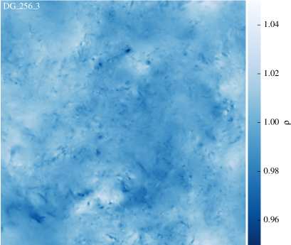
Figure 1: A thin slice through the middle of our best resolved DG simulation at third order showing the density field. The field uses the sub-cell information given by the high order DG weights. Every cell is sub-sampled four times

3.2 Dissipation measurement

We use an adiabatic index of $\gamma=1.01$ instead of the isothermal index $\gamma=1$. The slight deviation from $\gamma=1$ allows us to measure the dissipated energy while the dynamics of the fluid is essentially isothermal. After each timestep, the expected specific internal energy is computed as

$$\epsilon=\frac{c^{2}}{\gamma-1}\frac{\rho^{\gamma-1}}{\rho_{0}^{\gamma-1}},$$ (37)

with sound speed $c$ and reference density $\rho_{0}=1$. This specific internal energy is enforced at all quadrature points within a cell. Thus, the weights associated with the total energy density using the kinetic momentum and density field have to be adjusted:

$$w_{\mathrm{e},l}^{K}(t)= \int_{K}\!\left(\frac{1}{2}\frac{\vec{p}(\vec{x},t)^{2}}{\rho(\vec{x},t)}+\rho(\vec{x},t)\epsilon(\vec{x},t)\right)\phi_{l}^{K}({\vec{x}})\,\mathrm{d}V$$

$$= \frac{|K|}{8}\int_{[-1,1]^{3}}\!\left(\frac{1}{2}\frac{\vec{p}(\vec{\vec{\xi}},t)^{2}}{\rho(\vec{\xi},t)}+\rho(\vec{\xi},t)\epsilon(\vec{\xi},t)\right)\phi_{l}(\vec{\xi})\,\mathrm{d}\vec{\xi}$$

$$\cong \frac{|K|}{8}\sum_{q=1}^{(k+1)^{3}}\!\left(\frac{1}{2}\frac{\vec{p}(\vec{\vec{\xi}_{q}},t)^{2}}{\rho(\vec{\xi}_{q},t)}+\rho(\vec{\xi}_{q},t)\epsilon(\vec{\xi}_{q},t)\right)\phi_{l}(\vec{\xi}_{q})\omega_{q}.$$ (38)

Afterwards, the average internal energy density in the cell can be recomputed as

$$\rho\epsilon={w_{\mathrm{e},0}^{K}}-\frac{1}{2}\frac{{\vec{w}_{\mathrm{p},0}^{K}}^{2}}{w_{\mathrm{\rho},0}^{K}}.$$ (39)

The dissipated energy is given by the difference between the average internal energy before and after adjusting the weights of the total energy density. Afterwards the positivity limiter is applied to guarantee non-negative values in our DG simulations.

3.3 Power spectrum measurement

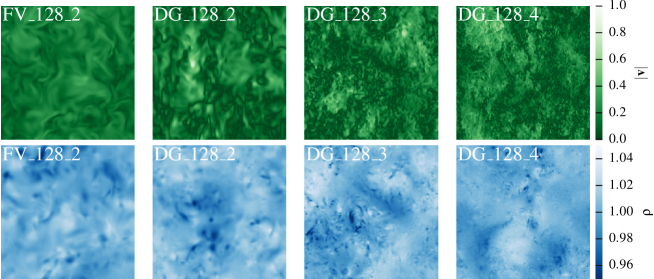
Figure 2: Thin slices through the density and velocity field at $t=30$. We compare the finite volume simulations against DG simulations of order 2 up to 4. Already 2nd order DG shows features which are finer than in the 2nd order finite volume run. The higher moments available in 3rd and 4th order DG allow a representation of finer features without increasing the spatial resolution. The thin lines of zero velocity are much more pronounced in case of DG than in the finite volume case

The power spectrum of a scalar or vector field $w(\vec{x})$ is proportional to the Fourier transformed of the two point correlation function:

$$C_{w}(\vec{l})=\langle w(\vec{x}+\vec{l})w(\vec{x})\rangle_{\vec{x}}.$$ (40)

Thus

$$E_{w}(\vec{k}) =(2\pi)^{3/2}\mathcal{F}(C_{w}(\vec{l}))=\int_{V}C_{w}(\vec{l})\exp(-i\vec{k}\vec{l})\,{\mathrm{d}}^{3}\vec{l}$$ (41)

$$=\left|\hat{w}({\vec{k}})\right|^{2},$$ (42)

where $\hat{w}$ is the Fourier transform of $w$. Here, we are only interested in the 1D power spectrum, thus we average $E_{w}({\vec{k}})$ over spherical shells:

$$E_{w}(k)=4\pi k^{2}\langle E_{w}({\vec{k}})\rangle,$$ (43)

where $k=\left|{\vec{k}}\right|$. The overall normalization of the Fourier transformation is chosen such that the integral over the power spectrum is equivalent to the total energy:

$$\sigma^{2}=\int w(x)\,{\mathrm{d}}\vec{x}=\int E_{w}(k)\,{\mathrm{d}}k=\frac{1}{(2\pi)^{3}N^{3}}\sum_{i,j,k=0}^{N-1}|\hat{w}_{ijk}|^{2},$$ (44)

with $\hat{w}_{ijk}$ being the discrete Fourier transformation of the discretized continuous field $w$. Usually we show $kE(k)$ instead of $E(k)$ directly in log-log plots. This means a horizontal line in a log-log plot represents equal energy per decade and makes interpreting the area under a curve easier.

4 Results

In Fig. 2 we show a first visual overview of our simulation results at a resolution of $128^{3}$ cells. The panels show the state at the final output time $t=30$ for the magnitude of the velocity and the density in a thin slice through the middle of the box. Each cell is subsampled four times for this plot using the full sub-cell information present for each DG or finite volume cell. In the case of the finite volume scheme, we used the estimated gradients in sub-sampling the cells.

The finite volume and DG results are similar at second order accuracy. However, already the second order DG run visually shows more small scale structure than the finite volume run. By increasing the order of accuracy and therefore allowing for more degrees of freedom within a cell, DG is able to represent considerably more structure at the same number of cells. Interestingly, the velocity field has regions of (almost) zero velocity. These thin stripes can be well represented in DG. The finite volume run shows the same features, but they are not as pronounced. Additionally, Fig. 1 shows a thin density slice for our highest resolution DG run DG_256_3. The high resolution and third order accuracy allows for more small scale details than in any other of our simulations.

4.1 Mach number evolution

t]

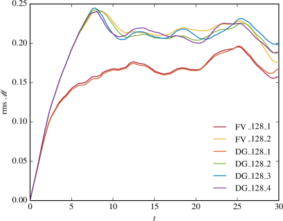
Figure 3: Time evolution of the root mean square Mach number $\mathcal{M}$. The runs with a higher than first order convergence order agree well with each other and establish a Mach number of about $\mathcal{M}\sim 0.2$ at $t=12$ in the quasi-stationary phase. However, the first order finite volume and DG runs do not manage to reach the same Mach number and fall substantially short of achieving a comparable kinetic energy throughout the entire run time

All of our runs with a convergence order larger or equal to second order reach an average Mach number of $\mathcal{M}\sim 0.21$ after $t=12$. The detailed history of the Mach number varies a bit from run to run. The differences between the different DG runs and finite volume runs are however insignificant. The same holds true for the other runs not shown in Fig. 3. Interestingly, both, the first order finite volume and DG runs fall substantially behind and can only reach a steady state Mach number of about $\mathcal{M}\sim 0.17$. The low numerical accuracy leads to a too high numerical dissipation rate in this case, preventing a fully established turbulent cascade. A similar problem was found in Bauer2012 for simulations with standard SPH even at comparatively high resolution, caused by a high numerical viscosity the noisy character of SPH.

4.2 Injected and dissipated energy

t]

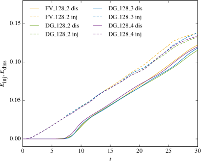
Figure 4: The dashed lines show the injected energy, while the solid lines give the dissipated energy over time. Dissipation becomes only relevant after an initial start-up phase. Thereafter, a quasi-stationary state is established

The globally injected and dissipated energy in our turbulence simulations is shown in Fig. 4 as a function of time. The rate of energy injection through the driving forces stays almost constant over time. At around $t=12$, the variations start to increase slightly. At this point the fluctuations between individual runs start to grow as well. Initially, the dissipation is negligible, but at around $t=8$ dissipation suddenly kicks in at a high rate, and then quickly transitions to a lower level at around $t=12$, where a quasi stationary state is reached that persists until the end of our runs. The difference between both curves – the kinetic energy – remains rather constant after $t=12$. Thus, in the following we only use outputs after $t=12$ for our analysis.

4.3 Velocity power spectra

t]

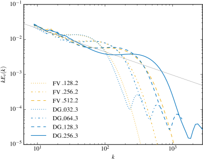
Figure 5: Comparison of the velocity power spectra of our second order finite volume runs against our third order DG runs. Interestingly, the spectra of the DG runs match with the ones obtained from the finite volume runs at a quarter of the resolution. Thus, DG obtains similar results using only about half as many degrees of freedom per dimension as finite volume schemes. For comparison, the grey line shows the $k^{-5/3}$ Kolmogorov scaling

In Fig. 5 and 6, we show velocity power spectra of our runs. First, we focus on a resolution study of our third order DG and second order finite volume simulations in Fig. 5. In case of the finite volume runs, we show the power spectra up to the Nyquist frequency $k_{n}=2\pi N/2L$, with $N$ being the number of cells per dimension. For our DG runs we show the full power spectrum instead, obtained from the grid used in the Fourier transformation up to $k_{g}=2\pi 4N/2L=4k_{n}$. The finite volume runs have a second peak not shown here at modes above $k_{n}$, induced by noise resulting from the discontinuities across cell boundaries. The third and higher order DG methods show a still declining power spectrum at $k_{n}$ and only at even higher modes close to $k_{g}$ start to show a noise induced rise. This is due to the available sub-cell information encoded in the DG weights.

All runs show an inertial range at scales smaller than the driving range on large scales. The inertial range is followed by a numerical dissipation bottleneck. This bottleneck is similar to the experimentally observed physical bottleneck effect, but appears to be somewhat stronger. The energy transfered to smaller scales can not be dissipated fast enough at the resolution scale and piles up there before it is eventually transformed to heat. The bottleneck feature moves to ever smaller scales as the numerical resolution is increased. Especially our highest resolution DG run $DG\_256\_3$ shows a quite large inertial range. However, the slope of the inertial range is measured slightly steeper than the expected $k^{-5/3}$ Kolmogorov scaling. We think a Mach number of $\mathcal{M}\sim 0.21$ and the associated density fluctuations are maybe already too high for a purely Kolmogorov-like turbulence cascade, which is only expected for incompressible gas.

Interestingly, the power spectra of our finite volume runs match those of our third order DG simulations, except that the finite volume scheme requires four times higher spatial resolution per dimension. Considering the $10$ degrees of freedom per cell for third order DG, the effective number of degrees of freedom is still lower by a factor of $6.4$ in the case of DG, which corresponds to a factor of $1.86$ per dimension. This underlines the power of higher order numerical methods, especially if comparatively smooth problems such as subsonic turbulence are studied.

t]

Figure 6: Velocity power spectrum for our DG runs at different convergence order at a resolution of $128^{3}$ cells. Already second order DG shows a large inertial range and a dissipation bottleneck at small scales. For comparison, the grey line shows the $k^{-5/3}$ Kolmogorov scaling

In Fig. 6 we compare the impact of the numerical convergence order on the power spectrum of our DG runs. As a comparison we include a second order finite volume run as well. All simulations have a numerical resolution of $128^{3}$. Already the second order DG method shows a more extended inertial range than the second order finite volume run. But the second order DG method already uses four degrees of freedom per cell. Increasing the convergence order alone improves the inertial range considerably. The change in going from second to third order is a bit larger than the change from third to fourth order.

4.4 Density PDFs

t]

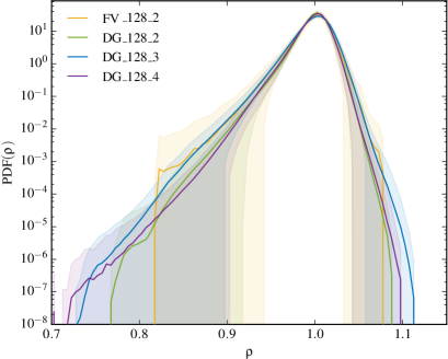
Figure 7: The density PDF for our runs at a resolution of $128^{3}$ cells. The PDF is obtained by subsampling each cell $4^{3}$ times. In the finite volume case, we take the estimated density gradients into account. For DG, we use the full polynomial information present in each cell. The shaded area represents the standard deviation over time. Interestingly, finite volume schemes show a sharp drop off at the low and high density ends which is absent in this form in the DG calculations

In Fig. 7, we show the probability density function (PDF) of the density field for some of our runs. The PDF is averaged from $t=12$ up to $t=30$ and sub-sampled $4^{3}$ times for each cell. We take the estimated density gradients into account for the finite volume runs. The finite volume run shows the smallest range of realized density values at the sampling points. Slightly more sampling points pile up at the extreme density values. This is due to the slope limited gradients used here, preventing more extreme density values. The DG runs show a more extended range of density values, with the range increasing with convergence order, because the higher order polynomial representations allow for a more detailed structure with more extrema within a cell. If only the mean values within the cells are considered, the PDFs are all rather similar to each other and not so different from the finite volume run shown.

5 Discussion

We presented the ideas and equations behind a new implementation of discontinues Galerkin hydrodynamics that we realized in the astrophysical simulation code TENET Schaal2015 . Unlike traditional finite volume schemes, DG uses subcell expansion into a set of basis functions, which leads to internal flux calculations in addition to surface integrals that are solved by a Riemann solver. Importantly, the reconstruction step needed in finite volume schemes is obsolete in DG. Instead, the coefficients of the expansion are evolved independently, and no information is ‘thrown away’ at the end of a timestep, unlike done by the implicit averaging in finite volume schemes at the end of every step. This offers the prospect of a higher computational efficiency, especially at higher order where correspondingly more information is retained from step to step. Such higher order can be relatively easily achieved in DG approaches. Furthermore, stencils only involve direct neighbours in DG, even for higher order, thereby making parallelization on distributed memory systems comparatively easy and efficient.

These advantages clearly make DG methods an interesting approach for discretizing the Euler equations. However, at shocks, the standard method may fall back to first order accuracy unless sophisticated limiters are used. If the problem at hand is dominated by shocks and discontinuities, this might be a drawback. Ultimately, only detailed application tests, like we have carried out here, can decide which method proves better in practice.

In this regard, an important question for comparing numerical methods is their computational efficiency for a given accuracy, or conversely, what is the best numerical accuracy which can be obtained for a given invested total runtime. Obtaining a fair comparison based on the run time of a code can be complicated in general. For example, for the runs analyzed in this study, different numbers of CPUs had to be used, as the memory requirements change by several orders of magnitude between our smallest and largest runs. The comparison may be further influenced by the fact that both hydro solver implementations investigated here are optimized to different degrees (with much more tuning already done for the finite volume method), which can distort simple comparisons of the run times. Nevertheless, we opted to give a straightforward comparison of the total CPU time used as a first rough indicator of the efficiency of our DG method compared to a corresponding finite volume scheme. We note however that our new DG code is less optimized thus far compared with the finite volume module, so we expect that there is certainly room for further improving the performance ratio in favor of DG.

We performed our simulations running in parallel on up to 4096 cores on SUPERMUC. In part thanks to the homogenous Cartesian mesh used in these calculations, our code showed excellent strong parallel scaling. We note that this is far harder to achieve when the adaptive mesh refinement (AMR) option present in TENET is activated.

We have generally found that the DG results for subsonic turbulence are as good as the finite volume ones, but only need slightly more than half as many degrees of freedom for comparable accuracy. Both the finite volume method at second order accuracy and the DG scheme at third order accuracy show very good weak scaling when increasing the resolution for the range of resolutions studied here. If we compare the run time for roughly equal turbulence power spectra, we find that the DG_032_3 run is about $1.14$ times faster than the corresponding FV_128_2 run. This performance ratio increases if we improve the resolutions: The DG_064_3 is already $1.34$ times faster than the FV_256_2 run. The DG_128_3 run is $1.53$ times faster than the FV_512_2 run, which comes close to the factor $1.86$ more degrees of freedom needed in the finite volume run to achieve the same accuracy. Thus, DG does not only need fewer degrees of freedom to obtain the same accuracy but also considerably less run time. This combination makes DG a very interesting method for solving the Euler equations.

Besides improving computational efficiency, DG has even more to offer. In particular, it can manifestly conserve angular momentum in smooth parts of the flow, unlike traditional finite volume methods. In addition, the ${\rm div}\vec{B}=0$ constraint of ideal magnetohydrodynamics (MHD) can be enforced at the level of the basis function expansion, opening up new possibilities to robustly implement MHD Mocz2014 . Combined with its computational speed, this reinforces the high potential of DG as an attractive approach for future exascale application codes in astrophysics, potentially replacing the traditional finite volume scheme that are still in widespread use today.

- (1) R.S. Klessen, F. Heitsch, M.M. Mac Low, ApJ 535, 887 (2000). DOI 10.1086/308891
- (2) M.M. Mac Low, R.S. Klessen, Reviews of Modern Physics 76, 125 (2004). DOI 10.1103/RevModPhys.76.125
- (3) P. Schuecker, A. Finoguenov, F. Miniati, H. Böhringer, U.G. Briel, A&A 426, 387 (2004). DOI 10.1051/0004-6361:20041039
- (4) P. Colella, P.R. Woodward, Journal of Computational Physics 54, 174 (1984). DOI 10.1016/0021-9991(84)90143-8
- (5) W.H. Reed, T. Hill, Los Alamos Report LA-UR-73-479 (1973)
- (6) B. Cockburn, C.W. Shu, Mathematics of Computation 52(186), 411 (1989)
- (7) B. Cockburn, S.Y. Lin, C.W. Shu, Journal of Computational Physics 84, 90 (1989). DOI 10.1016/0021-9991(89)90183-6
- (8) B. Cockburn, S. Hou, C.W. Shu, Mathematics of Computation 54, 545 (1990). DOI 10.1090/S0025-5718-1990-1010597-0
- (9) B. Cockburn, C.W. Shu, RAIRO-Modélisation mathématique et analyse numérique 25(3), 337 (1991)
- (10) B. Cockburn, C.W. Shu, Journal of Computational Physics 141, 199 (1998). DOI 10.1006/jcph.1998.5892
- (11) B. Cockburn, G. Karniadakis, C. Shu, Discontinuous Galerkin Methods: Theory, Computation and Applications. Lecture Notes in Computational Science and Engineering (Springer Berlin Heidelberg, 2011)
- (12) J.P. Gallego-Valencia, J. Löbbert, S. Müthing, P. Bastian, C. Klingenberg, Y. Xia, PAMM 14(1), 953 (2014). DOI 10.1002/pamm.201410457
- (13) P. Mocz, M. Vogelsberger, D. Sijacki, R. Pakmor, L. Hernquist, MNRAS 437, 397 (2014). DOI 10.1093/mnras/stt1890
- (14) O. Zanotti, F. Fambri, M. Dumbser, MNRAS 452, 3010 (2015). DOI 10.1093/mnras/stv1510
- (15) A. Bauer, V. Springel, MNRAS 423, 2558 (2012). DOI 10.1111/j.1365-2966.2012.21058.x
- (16) J.W. Wadsley, G. Veeravalli, H.M.P. Couchman, MNRAS 387, 427 (2008). DOI 10.1111/j.1365-2966.2008.13260.x
- (17) D.J. Price, Journal of Computational Physics 227, 10040 (2008). DOI 10.1016/j.jcp.2008.08.011
- (18) S. Heß, V. Springel, MNRAS 406, 2289 (2010). DOI 10.1111/j.1365-2966.2010.16892.x
- (19) J.I. Read, T. Hayfield, O. Agertz, MNRAS 405, 1513 (2010). DOI 10.1111/j.1365-2966.2010.16577.x
- (20) T. Abel, MNRAS 413, 271 (2011). DOI 10.1111/j.1365-2966.2010.18133.x
- (21) P.F. Hopkins, MNRAS 428, 2840 (2013). DOI 10.1093/mnras/sts210
- (22) K. Schaal, A. Bauer, P. Chandrashekar, R. Pakmor, C. Klingenberg, V. Springel, MNRAS 453, 4278 (2015). DOI 10.1093/mnras/stv1859
- (23) B.G. Galerkin, Vestnik Inzh. 19, 897 (1915)
- (24) S. Gottlieb, C.W. Shu, E. Tadmor, SIAM review 43(1), 89 (2001)
- (25) X. Zhang, C.W. Shu, Journal of Computational Physics 229, 8918 (2010). DOI 10.1016/j.jcp.2010.08.016
- (26) W. Schmidt, W. Hillebrandt, J.C. Niemeyer, Computers & Fluids 35(4), 353 (2006). DOI 10.1016/j.compfluid.2005.03.002
- (27) C. Federrath, R.S. Klessen, W. Schmidt, ApJ 688, L79 (2008). DOI 10.1086/595280
- (28) C. Federrath, R.S. Klessen, W. Schmidt, ApJ 692, 364 (2009). DOI 10.1088/0004-637X/692/1/364
- (29) C. Federrath, J. Roman-Duval, R.S. Klessen, W. Schmidt, M.M. Mac Low, A&A 512, A81 (2010). DOI 10.1051/0004-6361/200912437
- (30) D.J. Price, C. Federrath, MNRAS 406, 1659 (2010). DOI 10.1111/j.1365-2966.2010.16810.x