Pricing and Hedging GMWB in the Heston and in the Black-Scholes with Stochastic Interest Rate Models

Abstract

Valuing Guaranteed Minimum Withdrawal Benefit (GMWB) has attracted significant attention from both the academic field and real world financial markets. As remarked by Yang and Dai [17], the Black and Scholes framework seems to be inappropriate for such a long maturity products. Also Chen Vetzal and Forsyth in [10] showed that the price of these products is very sensitive to interest rate and volatility parameters. We propose here to use a stochastic volatility model (Heston model) and a Black Scholes model with stochastic interest rate (Hull White model). For this purpose we present four numerical methods for pricing GMWB variables annuities: a hybrid tree-finite difference method and a Hybrid Monte Carlo method, an ADI finite difference scheme, and a Standard Monte Carlo method. These methods are used to determine the no-arbitrage fee for the most popular versions of the GMWB contract, and to calculate the Greeks used in hedging. Both constant withdrawal, optimal surrender and optimal withdrawal strategies are considered. Numerical results are presented which demonstrate the sensitivity of the no-arbitrage fee to economic, contractual and longevity assumptions.

Keywords: Variable Annuities, stochastic volatility, stochastic interest rate, optimal withdrawal.

1 Introduction

Variable Annuities are investment contracts with insurance coverage. In recent years, they become a source of attraction for many investors, because of their specific features: they are tax-deferral products able to guarantee a minimum return for a long period, and to take advantage of favorable market movements. The models in the literature, present the analysis of these products in the Black and Scholes model, disregarding possible changes in the interest rate and the volatility of the underlying.

In 2008 following the subprime crisis, financial markets have suffered the upheavals that have affected the entire world economy. Since then, these markets were extremely volatile. After many failures, the gap between the different interest rates applied to different transmitters has become larger and larger, and a discussion on the identification of the risk-free rate is open. The ECB and the Fed’s interest rates gradually declined, while the rate on sovereign debt increased gradually.

In this article, we consider a Guaranteed Minimum Withdrawal Benefit (GMWB) annuity. We restrict our attention to a simplified form of a GMWB which is initiated by making a lump sum payment to an insurance company. This lump sum is then invested in risky assets, usually a mutual fund. The benefit base, or guarantee account balance, is initially set to the amount of the lump sum payment. The holder of the policy (hereinafter, we will abbreviate it with PH) is entitled to withdraw a fixed sum, even if the actual investment in the risky asset declines to zero. The withdrawal period may start immediately or later: in this case the benefit base and the account value may be reset to the maximum between their value and a fixed value. Finally, the PH may withdraw more than the contractually specified amount, including complete surrender of the contract, upon payment of a penalty. Complete surrender here means that the PH withdraws the entire amount remaining in the investment account, and the contract terminates. In most cases, this penalty for full or partial surrender declines to zero after five to seven years. During contract execution, a death benefit may come with the PH’s death: in this case, his (her) heirs receive the remaining amount in the risky asset account.

The hedging costs for this guarantee are offset by deducting a proportional fee from the risky asset account. From an insurance point of view, these products are treated as financial ones: the products are hedged as if they were pure financial products, and the mortality risk is hedged using the law of large numbers. Therefore, it’s very important for insurance companies to be able to price quickly these products. Moreover these products have long maturities that could last almost 25 years. The Black-Scholes model, with constant interest rate and volatility seems to be unsuitable for those products: that’s why we present our pricing methods in two frameworks, modeling stochastic volatility (Heston model [15]) and stochastic interest rate (Hull-White model [16]) .

There have been several recent articles on pricing GMWBs. In particular, we would remember Chen and Forsyth [9] and Chen, Vetzal and Forsyth [10]. In the first paper, the authors used an impulse stochastic control formulation for pricing variable annuities GMWB, assuming the PH to be allowed to withdraw funds continuously, or only at anniversaries. In the second one, the authors analyzed the impact of several product and model parameters using the same PDE approach. The use of PDEs proved to be very fast and accurate, and we used it as a reference for our work.

Another research work about GMWB is Yang and Dai’s one [17]: they used a flexible tree for evaluating GMWB contracts with various provisions. Yang-Dai’s product is slightly different from Chen-Forsyth’s one: that’s why we treat the two apart.

We have made reference also to Bacinello et al. [4]: variable annuities (including GMWBs) are priced using a Monte Carlo approach. The PH’s behavior is assumed to be semi-static, i.e. the holder withdraws at the contract rate or surrenders the contract.

In this paper, we price two types of GMWBs guarantees and we find the no-arbitrage fee in the Heston model and the Black-Scholes with stochastic interest rate model (BS HW model). First, we treat a static withdrawal strategy: the PH withdraws at the contract rate. Then, taking the point of view of the worst case for the hedger, we price the guarantees assuming that the PH follows a dynamic withdrawal strategy. We also used these methods to calculate the Greeks for hedging and risk management. For this purpose we present four numerical methods: a hybrid tree-finite difference method and a Hybrid Monte Carlo method (both introduced by Briani et al. [6]) an ADI finite difference scheme (Haentjens and Hout [14]), and a Standard Monte Carlo method with Longstaff-Schwartz least squares regression (Longstaff and Schwartz [18]). These methods have already been developed in the problem of “Guaranteed Lifelong Withdrawal Benefit” (GLWB) pricing as we did in [13], but in this case problem dimension may change. In fact, GLWB pricing problem has dimension equal to 2, while GMWB pricing problem may have dimension 2 or 3.

We use the term no-arbitrage fee in the sense that this is the fee which is required to maintain a replicating portfolio. A description of the replicating portfolio for these types of guarantees is given in Chen et al. [9] and Belanger et al. [5].

The main results of this paper are the following ones:

• We formulate the determination of the no-arbitrage fee (i.e. the cost of maintaining a replicating hedging portfolio) in the Heston model and in the BS HW model using different pricing methods;

• We present the effects of stochastic volatility and stochastic interest rate on pricing and Greeks calculation, and the sensitivity of the GMWB fee to various modeling parameters;

• We use different numerical methods to price the GMWB contracts;

• We present numerical examples which show the convergence of these methods.

The paper is organized as follows: in Section 2, we describe the main features of the contracts such as event times, withdrawals and penalties. In Section 3, we provide a brief review of the stochastic models used afterward. In Section 4, we present the numerical methods, and how to implement them to solve the GMWB contract pricing problem. In Section 5 we perform numerical tests in order to show their behavior and we study the sensitivity of the no-arbitrage fee to economic and contractual assumptions. Finally, in Section 6, we present the conclusions.

2 The GMWB Contracts

In the following, we will refer to the contracts described in the paper of Chen and Forsyth [9] and in the paper of Yang and Dai [17]. We are calling GMWB-CF the contract described in [9] and GMWB-YD the contract described in [17]. Now, we make a brief summary of the main features of the two contracts.

2.1 Mortality

Similar to the work of Chen and Forsyth [9], Milevsky and Salisbury [19] and Dai et al. [11], we will ignore mortality effects in the following. We plan to study the effects of mortality in a future work.

2.2 Contract State Parameters

At time $t=0$ the policy holder pays with lump sum the premium $P$ to the insurance company. The premium $P$ is invested in a fund whose price is denoted by the variable $S_{t}$.

For both the two contracts, we suppose that there is a set of discrete times $\left\{t_{i},i=1,\dots N\right\}$, which we term event times; at these times withdrawals may occur. We suppose $\Delta t_{i}=t_{i+1}-t_{i}$ to be constant, and denoted by $\Delta t$. We also consider $t_{0}=t_{1}-\Delta t$, and to be consistent with Yang Dai’s notation we will write $T_{1}$ instead of $t_{0}$ ($T_{1}=t_{0}$). Then, we write $T_{1}<T_{1}+\Delta t=t_{1}<t_{2}<\dots<t_{N}=T_{2}$; the time interval $\left[T_{1},T_{2}\right]$ is called payout phase. We remark that no withdrawals take place in $T_{1}$.

GMWB-CF

The state parameters of the contract are:

• Account value: $A_{t}$, $A_{0}=P$.

• Base benefit: $B_{t}$, $B_{0}=P$.

Both these two variables are initially set equal to the premium. We define $T_{1}=0$ the time of the contract beginning, and $T_{2}=t_{N}$ the time of the last possible withdrawal. Usually, the first withdrawal takes place in $t_{1}=1\ y$ or $t_{1}=0.5\,y$.

GMWB-YD

The state parameters of the contract are:

• Account value: $A_{t}$, $A_{0}=P$.

• Guaranteed minimum withdrawal: $G$.

The variable $A_{t}$ is initially set equal to the premium, while $G$ is not defined until the beginning of the withdrawal period at time $T_{1}$. For this type of contract we don’t need to define the Benefit Base variable because its value is deterministic until the PH decides to lapse.

For this product, there exist two time parameters, $T_{1}$ and $T_{2}$ that express the begin and the end of the payout phase. Yang and Dai used integers values for $T_{1}$ and $T_{2}$ and $\Delta t=1\,y$ in their numerical tests. No withdrawals happen during the deferred time, i.e. for $t\in\left[0,T_{1}\right[$: in that period the account value evolves as explained in the next subsection (see Formula (2.2)). At time $T_{1}$ also the account value is reset to

$$A_{T_{1}^{\left(+\right)}}=\max\left[C\left(T_{1}\right),A_{T_{1}^{\left(-\right)}}\right],$$

and the value of $G$ is fixed as

$$G=\frac{A_{T_{1}^{\left(+\right)}}}{m\left(T_{2}-T_{1}\right)},$$ (2.1)

where $m$ denotes the number of withdrawals per year (usually $m=1$), and $C\left(T_{1}\right)$ is a contract specified value that can be interpreted as the lower bound of the total guaranteed withdrawal. That value is specified as the return on the initial investment with a roll-up interest rate guaranteed interest rate $i$, as follows:

$$C\left(T_{1}\right)=P\left(1+i\right)^{T_{1}}.$$

If $T_{1}=0$, the reset is trivial: $A_{T_{1}^{\left(+\right)}}=A_{0}=P$.

2.3 Evolution of the Contracts in the Deferred Time and between Event Times.

We call deferred time the time between $0$ and the beginning of the payoff phase $T_{1}$: $0\leq t<T_{1}$. This time set is empty unless for deferred GMWB-YD products; the other products have $T_{1}=0$ so there is no deferred time. We first consider the evolution of the value of the guarantee excluding event times $t_{i}$. Let $t\in\left[0,T_{1}\right[\subseteq\left[0,T_{2}\right]$ or $t\in\left]t_{i},t_{i+1}\right[\subseteq\left[0,T_{2}\right]$. As we said before, $S_{t}$ denotes the underlying fund driving the account value. The dynamics of $S_{t}$ will be described in the next Section. The account value $A_{t}$ follows the same dynamics of $S_{t}$ with the exception of the fact that some fees may be subtracted continuously:

$$dA_{t}=\frac{A_{t}}{S_{t}}dS_{t}-\alpha_{tot}A_{t}dt.$$ (2.2)

We suppose that the total annual fees are charged to the PH and withdrawn continuously from the investment account $A_{t}$. These fees include the mutual fund management fees $\alpha_{m}$ and the fee charged to fund the guarantee (also known as the rider) $\alpha_{g}$, so that

$$\alpha_{tot}=\alpha_{m}+\alpha_{g}.$$

The only portion used by the insurance company to hedge the contract is that coming from $\alpha_{g}$: the other part of the fees has to be considered as an outgoing money flow as PH’s withdrawals are.

2.4 Event Times and Final Payoff

Let $G$ be the withdrawal guaranteed amount: for a CF product type, this parameter is a contract input, while for a YD type this value is determined at time $T_{1}$ according to formula 2.1.

We denote $W_{i}$ the withdrawal of the PH at time $t_{i}$. As in [9], we observe that $W_{i}$ is a control variable.

GMWB-CF

Usually the first event time takes place at time $t_{1}=\Delta t=1\,y$ or $t_{1}=\Delta t=0.5\,y$ ; moreover $t_{i}=i\cdot\Delta t$.

We denote with $\left(A_{t_{i}^{\left(-\right)}},B_{t_{i}^{\left(-\right)}},t_{i}\right)$ the state variables just before an event time that occurs at time $t_{i}$ and with $\left(A_{t_{i}^{\left(+\right)}},B_{t_{i}^{\left(+\right)}},t_{i}\right)$ the state variables just after it.

We distinguish two pricing frameworks: at each event time the PH can withdraw according to the contract rate $G$ (Static approach) or to a different rate (Dynamic approach). If $W_{i}\leq G$, then there is no penalty imposed; if $W_{i}>G$ there is a proportional penalty charge $\kappa\left(W_{i}-G\right)$. Anyway, the value of $W_{i}$ chosen by the PH cannot exceed the guaranteed withdrawal amount $B_{t_{i}^{\left(-\right)}}$: it must be $W_{i}\in\left[0,B_{t_{i}^{\left(-\right)}}\right]$.

As we said before, the PH may not receive all the money he (she) withdraws from the account value. Let $f_{i}\left(W\right):\left[0,B_{t_{i}^{\left(-\right)}}\right]\rightarrow\mathbb{R}$ be a function of $W_{i}$ denoting the rate of cash flow received by the PH due to the withdrawal at time $t_{i}$. Then,

$$f_{i}\left(W_{i}\right)=\begin{cases}W_{i}&\mbox{if }W_{i}\leq G\\ W_{i}-\kappa\left(W_{i}-G\right)&\mbox{if }W_{i}>G.\end{cases}$$

The new state variables are

$$\left(A_{t_{i}^{\left(+\right)}},B_{t_{i}^{\left(+\right)}},t_{i}\right)=\left(\max\left(A_{t_{i}^{\left(-\right)}}-W_{i},0\right),B_{t_{i}^{\left(-\right)}}-W_{i},t_{i}\right).$$ (2.3)

At time $t=T_{2}$ the last event time takes place: the PH withdraws as in the previous event times; then he (she) receives the final payoff which is worth

$$FP=\max\left(A_{T_{2}},\left(1-\kappa\right)B_{T_{2}}\right).$$

This final payoff is applied also in the static case.

It is possible to prove that the optimal withdrawal at time $T_{2}$ is $W_{N}=\min\left(G,B_{T_{2}^{\left(-\right)}}\right)$; in this case, the value of the contract before the withdrawal is

$$\mathcal{V}\left(A_{T_{2}^{\left(-\right)}},B_{T_{2}^{\left(-\right)}},T_{2}\right)=\max\left(A_{T_{2}^{\left(-\right)}},\left(1-\kappa\right)B_{T_{2}^{\left(-\right)}}+\kappa\min\left(G,B_{T_{2}^{\left(-\right)}}\right)\right).$$

Therefore, this remark simplifies the research of the optimal withdrawal in the Dynamic framework.

We notice that, if $A_{t_{i}^{\left(-\right)}}>B_{t_{i}^{\left(-\right)}}$ the contract can not be fully terminated in $t_{i}$: if the PH withdraws at the maximal rate, then $W_{i}=B_{t_{i}^{\left(-\right)}}$ and $\left(A_{t_{i}^{\left(+\right)}},B_{t_{i}^{\left(+\right)}},t_{i}\right)=\left(A_{t_{i}^{\left(-\right)}}-B_{t_{i}^{\left(-\right)}},0,t_{i}\right)$. In this case the PH won’t be able to make any withdrawal in following event times because of $B=0$, but he will receive the final payoff $FP=A_{T_{2}}$ at time $T_{2}$.

GMWB-YD

This kind of products can be deferred or not. If we set $\Delta t=\nicefrac{{\left(T_{2}-T_{1}\right)}}{{N}}$, then $t_{i}=T_{1}+\Delta t\cdot i$ for $i=1,\dots,N$. Usually $\Delta t=1\,y$.

We denote with $\left(A_{t_{i}^{\left(-\right)}},G^{\left(-\right)},t_{i}\right)$ the state variables just before an event time that occurs at time $t_{i}$ and with $\left(A_{t_{i}^{\left(+\right)}},G^{\left(+\right)},t_{i}\right)$ the state variables just after it.

According to [17], we distinguish two pricing frameworks: at each event time the PH can withdraw according to the contract rate $G$ (Static approach) or fully surrender (Dynamic approach). In the first case, he (she) receives $G$ at all event times after $T_{1}$ ($T_{2}-T_{1}$ payments) and the state change is given by

$$\left(A_{t_{i}^{\left(+\right)}},G^{\left(+\right)},t_{i}\right)=\left(\max\left(0,A_{t_{i}^{\left(+\right)}}-G^{\left(-\right)}\right),G^{\left(-\right)},t_{i}\right).$$ (2.4)

At time $t=T_{2}$, the PH receives $G$ plus the final payoff:

$$FP=A_{T_{2}^{\left(+\right)}}.$$

In the second case, the PH receives $G$ until the surrender event, and the equation (2.4) still holds. Let’s suppose that the PH decides to surrender at time the event time $t_{i^{*}}$; then

$$\left(A_{t_{i^{*}}^{\left(+\right)}},G,t_{i^{*}}\right)=\left(0,0,t_{i^{*}}\right).$$

The final payoff is paid out at time $t_{i^{*}}$, and the contract becomes valueless:

$$FP=G+\left(1-\kappa\right)\max\left(0,A_{t_{i^{*}}^{\left(-\right)}}-G\right).$$

2.5 Similarity Reduction

An important property of GMWB-YD contract is the fact that this contract behaves good under scaling transformations as also GLWB variable annuities do. If $\mathcal{V}\left(A,G,t\right)$ denotes the value of a contract, it is possible to prove that for any scalar $\eta>0$

$$\eta\mathcal{V}\left(A,G,t\right)=\mathcal{V}\left(\eta A,\eta G,t\right).$$ (2.5)

Then, we just have to treat the case $G=\hat{G}$ for a fixed value $\hat{G}$ (for example $\hat{G}=P/\left(T_{2}-T_{1}\right)$), and then, choosing $\eta=\nicefrac{{\hat{G}}}{{G}}$, we can obtain

$$\mathcal{V}\left(A,G,t\right)=\frac{G}{\hat{G}}\mathcal{V}\left(\frac{\hat{G}}{G}A,\hat{G},t\right),$$

which means that we can solve the pricing problem only for a single representative value of $G$. This effectively reduces the problem dimension.

The previous property can be applied at time $T_{1}$ when $A$ and $G$ are reset. Some simple calculations show that

$$\mathcal{V}\left(A_{T_{1}^{\left(+\right)}},G_{T_{1}}^{+},T_{1}\right)=\frac{A_{T_{1}^{\left(+\right)}}}{P}\mathcal{V}\left(P,\hat{G},T_{1}\right).$$

The similarity reduction (2.5) was also exploited from Shah et Bertsimas in [22]. We would remark that Yang and Dai didn’t use this technique for their product: therefore, their resolution of the problem of pricing is more complicated and computationally expensive.

According to GMWB-CF contracts, the similarity reduction can’t be applied directly. In fact, we can prove that

$$\eta\mathcal{V}\left(A,B,G,t\right)=\mathcal{V}\left(\eta A,\eta B,\eta G,t\right)$$ (2.6)

but in this case we have to scale also the guaranteed withdrawal amount $G$ and therefore it is not useful to reduce problem dimension.

3 The Stochastic Models of the Fund $S$

To understand the different impacts of stochastic volatility and stochastic interest rate over such a long maturity contract, we price the GMWB VA according to two models: the Heston model, which provides stochastic volatility, and the Black-Scholes Hull-White model, which provide stochastic interest rate. As we said before, the process $S$ represents the underlying fund driving the account value $A_{t}$ of the product.

3.1 The Heston Model

The Heston model [15] is one of the most known and used models in finance to describe the evolution of the volatility of an underlying asset and the underlying asset itself. In order to fix the notation, we report its dynamics:

$$\begin{cases}dS_{t}=rS_{t}dt+\sqrt{v_{t}}S_{t}dZ_{t}^{S}&S_{0}=\bar{S}_{0},\\ dv_{t}=k\left(\theta-v_{t}\right)dt+\omega\sqrt{v_{t}}dZ_{t}^{v}&v_{0}=\bar{v}_{0},\end{cases}$$ (3.1)

where $Z^{S}$ and $Z^{v}$ are Brownian motions, and $d\left\langle Z_{t}^{S},Z_{t}^{v}\right\rangle=\rho dt$.

3.2 The Black-Scholes Hull-White Model

The Hull-White model [16] is one of historically most important interest rate models, which is nowadays often used for risk-management purposes. The important advantage of the HW model is the existence of closed formulas to calculate the prices of bonds, caplets and swaptions. In order to fix the notation, we report the dynamics of the BS HW model:

$$\begin{cases}dS_{t}=r_{t}S_{t}dt+\sigma S_{t}dZ_{t}^{S}&S_{0}=\bar{S}_{0},\\ dr_{t}=k\left(\theta_{t}-r_{t}\right)dt+\omega dZ_{t}^{r}&r_{0}=\bar{r}_{0},\end{cases}$$

where $Z^{S}$ and $Z^{r}$ are Brownian motions, and $d\left\langle Z_{t}^{S},Z_{t}^{r}\right\rangle=\rho dt$.

The process $r$ is a generalized Ornstein-Uhlenbeck (hereafter OU) process: here $\theta_{t}$ is not constant but it is a deterministic function which is completely determined by the market values of the zero-coupon bonds (ZCBs) by calibration (see Brigo and Mercurio [8]): in this case the theoretical prices of the ZCBs match exactly the market prices.

Let $P^{M}\left(0,T\right)$ denote the market price of the ZCB at time $0$ for the maturity $T$. The market instantaneous forward interest rate is then defined by

$$f^{M}\left(0,T\right)=-\frac{\partial\ln P^{M}\left(0,T\right)}{\partial T}.$$

It is well known that the short rate process $r$ can be written as

$$r_{t}=\omega X_{t}+\beta\left(t\right),$$

where $X$ is a stochastic process given by

$$dX_{t}=-kX_{t}dt+dZ_{t}^{r},\ X_{0}=0,$$

and $\beta\left(t\right)$ is a function

$$\beta\left(t\right)=f^{M}\left(0,t\right)+\frac{\omega^{2}}{2k^{2}}\left(1-\exp\left(-kt\right)\right)^{2}.$$

Then, the BS HW model is described by

$$\begin{cases}dS_{t}=r_{t}S_{t}dt+\sigma S_{t}dZ_{t}^{S}&S_{0}=\bar{S}_{0},\\ dX_{t}=-kX_{t}dt+dZ_{t}^{r}&X_{0}=0,\\ r_{t}=\omega X_{t}+\beta\left(t\right).\end{cases}$$ (3.2)

A particular case is called flat curve. In this case, we assume $P^{M}\left(t,T\right)=e^{-\bar{r}_{0}\left(T-t\right)}$ and $f^{M}\left(0,T\right)=\bar{r}_{0}$. Then

$$\beta\left(t\right)=\bar{r}_{0}+\frac{\omega^{2}}{2k^{2}}\left(1-\exp\left(-kt\right)\right)^{2},$$

and

$$\theta_{t}=\bar{r}_{0}+\frac{\omega^{2}}{2k^{2}}\left(1-\exp\left(-2kt\right)\right).$$

4 Numerical Methods of Pricing

In this Section we describe the four pricing methods: a Hybrid Monte Carlo method, a Standard Monte Carlo method, a Hybrid PDE method, and an ADI PDE method.

We remember that our aim is to find the fair value for $\alpha_{g}$: it’s the charge that makes the initial value of the policy equal to the initial premium. To achieve this target, we price the policy (with one of the following procedures) and then we use the secant method to approach the correct value for $\alpha_{g}$. Therefore, the main goal is to be able to find the initial value for a given value of $\alpha_{g}$: $\mathcal{V}\left(A_{0},B_{0},0\right)\left(\alpha_{g}\right)$.

We remark that we want to calculate the value of the policy from the point of view of the insurance company: the management fees are treated as a outgoing cash flows, and if we assume that the policy holder follows a withdrawal strategy, we consider the worst one for the insurance company.

4.1 The Hybrid Monte Carlo Method

The value of a GMWB policy can be calculated through a Monte Carlo set of simulations. This procedure is based in two steps: generation of a scenario (a sampling of the underlying values along the life of the product), and projection of the product into the scenario. According to the way we obtain the scenarios, we distinguish two Monte Carlo models: Hybrid MC (HMC) and Standard MC (SMC).

The Hybrid MC method was introduced in Briani et al. [7]. It is a simple and efficient way to produce MC scenarios for different models. This method is called “hybrid” because it combines trees and MC methods. First, a simple tree needs to be built: this can be done according to Appolloni et al. [3] or, as we did for GLWB in [13]. Then, using a vector of Bernoulli random variables, we move from the root through the tree, describing the scenario for the volatility or the interest rate. The values of the underlying at each time step can be easily obtained using an Euler scheme.

4.1.1 Trees

In this Subsection, we present the main points useful to build a tree for volatility or interest rate: they’re simple quadrinomial trees, built to match the first 3 moments of the stochastic processes. Other trees can be built according to Appolloni et al. [3] or Nelson and Ramaswamy [20], but we preferred our quadrinomial trees because they give more guarantee of convergence to the exact price also for long maturities. An example of those trees is available in Figure 4.1.

We suppose to fix a time horizon $\left[0,T\right]$, a number $N>0$ and we define $h=\nicefrac{{T}}{{N}}$. We denote $\bar{G}_{\left(n,j\right)}$ the value of a node of tree level $n$ and position $j$.

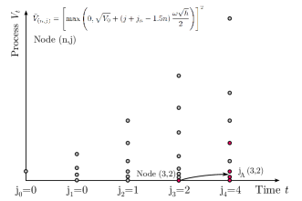
Figure 4.1: The trees for Heston and Hull-White models.

The Heston Model

The Heston process (3.1) for volatility has no constant variance and isn’t Gaussian. We consider the process obtained by the square root:

$$d\sqrt{v_{t}}=\frac{4k\left(\theta-\sqrt{v_{t}}^{2}\right)-\omega^{2}}{8\sqrt{v_{t}}}dt+\frac{\omega}{2}dZ_{t}.$$

We approximate it with a Gaussian process with variance $\frac{\omega^{2}}{4}dt$. This approximation is helpful to define the grid of states-space for the Markov chain: inspired by [20], we define

$$j_{n}=\max\left(0,\mbox{floor}\left(1.5n-\frac{2\sqrt{v_{0}}}{\omega\sqrt{h}}\right)\right),$$

and we set

$$\bar{v}_{\left(n,j\right)}=\left(\max\left(0,\sqrt{v_{0}}+\left(j+j_{n}-1.5n\right)\frac{\omega\sqrt{h}}{2}\right)\right)^{2}.$$

for $j=0,\dots,3n-j_{n}$. The shift due to $j_{n}$ helps to reject the many nodes with value equal to zero: if $j_{n}>0$, then $\bar{v}_{\left(n,0\right)}=0$ and $\bar{v}_{\left(n,1\right)}>0$ .

We would remark that the process $\bar{v}_{t}$ approximates $v_{t}$ and not $\sqrt{v_{t}}$: the moments matching is done according to the moments of the process $v_{t}$.

We fix now the values of $n$ and $j$. The discrete process $\bar{v}$ can jump from a node to another, as in a Markovian chain. We show now how to find the possible upcoming nodes.

The first three moments for the Heston process can be found in Alfonsi [1]:

$$\psi\left(h\right)=\nicefrac{{\left(1-e^{-kh}\right)}}{{k}},\ \ \ M_{1}=\mathbb{E}\left[v_{t+h}|v_{t}=v\right]=ve^{-kh}+\theta k\psi\left(h\right),$$

$$M_{2}=\mathbb{E}\left[\left(v_{t+h}\right)^{2}|v_{t}=v\right]=M_{1}^{2}+\omega^{2}\psi\left(h\right)\left[\theta k\psi\left(h\right)/2+ve^{-kh}\right],$$

$$M_{3}=\mathbb{E}\left[\left(v_{t+h}\right)^{3}|v_{t}=v\right]=M_{1}M_{2}+\omega^{2}\psi\left(h\right)\left[2v^{2}e^{-2kh}+\psi\left(h\right)\left(k\theta+\frac{\omega^{2}}{2}\right)\left(3ve^{-kh}+\theta k\psi\left(h\right)\right)\right].$$

Then, we can proceed as in the general case. Anyway, the grid we’re using is based on an approximation: so the probabilities obtained solving the linear system may not be positive. If we get a negative transition probability for a given node, we try another combination of out-coming nodes, replacing one (or two) of the nodes $A$, $B$, $C$, $D$ with one (or two) close to them. The nodes $A$ or $C$ may be replaced by a node $E$ defined as the first node bigger than $C$, and the nodes $B$ or $D$ may be replaced with a node $F$, defined as the smallest before node $D$. This gives rise to $9$ combinations to be tested. If the starting node is small and the node $D$ verifies $j_{D}=j_{n}$ we could not do this last change because there would be no $F$ node. In this case we allow the node $D$ to be replaced by the node $E$: see Figure 4.2.

Figure 4.2: The possible combinations used to get positive probabilities in the Heston model tree. The red points correspond to the used nodes.

If these attempts don’t give a positive result (negative probabilities), we give up trying to match the first three moments, and we are content to match an approximation of the first two as in [20], thus ensuring the weak convergence. In this case, we only use the nodes $A,B,C,D$: we define

$$p_{AB}=\frac{\mu-G_{n+1,j_{B}}}{G_{n+1,j_{A}}-G_{n+1,j_{B}}},\ \ p_{BA}=1-p_{AB},$$

$$p_{CD}=\frac{\mu-G_{n+1,j_{D}}}{G_{n+1,j_{C}}-G_{n+1,j_{D}}},\ \ p_{DC}=1-p_{CD},$$

and

$$p_{A}=\frac{5}{8}p_{AB},\ p_{B}=\frac{5}{8}p_{BA},\ p_{C}=\frac{3}{8}p_{CD},\ p_{D}=\frac{3}{8}p_{DC}.$$

It is possible to show that the first moment of this variable is equal to $M_{1}$, and as $h\rightarrow 0$ the second moment approaches to $M_{2}$, ensuring the convergence, as proved in [20].

In all our numerical tests, this last option (matching only two moments) has never been necessary: changing the nodes, all moments were matched with positive probabilities.

The Hull-White Model

The process $X$ in (3.2) is Gaussian, and this property simplifies the tree construction. As shown in Ostrovski [21] the variables $X_{t}$ and $\int_{s}^{t}X_{y}dy$ are bivariate normal distributed conditionally on $X_{s}$ with well known mean and variance. We define

$$X_{\left(n,j\right)}=\left(j-\frac{3n}{2}\right)\sqrt{\frac{1-\exp\left(-2kh\right)}{2k}},\ n=0,\dots,N\mbox{ and }j=0,\dots,3n.$$

Let’s fix a node $X_{\left(n,j\right)}$. We define

$$H=\exp\left(-kh\right),\ K=\sqrt{\frac{1-\exp\left(-2kh\right)}{2k}},\ M_{1}=X{}_{\left(n,j\right)}H,$$

$$j_{A}=\mbox{ceil}\left[\frac{M_{1}}{K}+\frac{3\left(n+1\right)}{2}\right],\ X_{A}=X_{\left(n+1,j_{A}\right)}.$$

The transition probabilities are given by

$$\begin{array}[]{cc}p_{A}=\frac{\left(X_{A}-M_{1}\right)}{2K^{3}}\left(K^{2}+\left(K+M_{1}-X_{A}\right)^{2}\right),&p_{B}=\frac{\left(K+M_{1}-X_{A}\right)}{2K^{3}}\left(K^{2}+\left(M_{1}-X_{A}\right)^{2}\right),\\ p_{C}=\frac{\left(K+M_{1}-X_{A}\right)}{6K^{3}}\left(2K^{2}+\left(K+M_{1}-X_{A}\right)^{2}\right),&p_{D}=\frac{\left(X_{A}-M_{1}\right)}{6K^{3}}\left(2K^{2}+\left(M_{1}-X_{A}\right)^{2}\right).\end{array}$$

4.1.2 Scenario Generation

The generations of the volatility process and of the interest rate process behaves in a similar way: we start from the node $\left(0,0\right)$ of the tree and according to a discrete random variable and to the node probabilities, we move to the next node and so on. Let $R$ be a discrete random variable that can assume value $A,B,C,D$ with probabilities $p_{A},p_{B},p_{C},p_{D}$: sampling such a variable at each node, we get the values of the process at each time step.

We distinguish two cases for the two models.

The Heston Model

We approximate the couple $\left(S_{t},v_{t}\right)$ in $\left[0,T\right]$ by a discrete process $\left(\bar{S}_{k\Delta t},\bar{v}_{k\Delta t}\right)_{k=0,\dots,T/\Delta t}$, with $\left(\bar{S}_{0},\bar{v}_{0}\right)=\left(S_{0},v_{0}\right)$. For each scenario, we generate the volatility.

Let $N\sim\mathcal{N}\left(0,1\right)$ and $B\sim\mathcal{B}\left(0.5\right)$. We deduce the value of $\bar{S}_{t+\Delta t}$ by

$$\bar{S}_{t+\Delta t}=\begin{cases}\bar{S}_{t}\exp\!\left[\!\left(r-\frac{\rho}{\sigma}k\theta\right)\!\Delta t\!+\!\left(\frac{\rho}{\sigma}k-\frac{1}{2}\right)\!\!\left(\!\frac{\bar{v}_{t+\Delta t}+\bar{v}_{t}}{2}\!\right)\!\Delta t\!+\!\frac{\rho}{\sigma}\!\left(\bar{v}_{t+\Delta t}-\bar{v}_{t}\right)\!+\!\sqrt{\!\left(1-\rho^{2}\right)\Delta t\bar{v}_{t}}N\!\right]&\mbox{if }B=0,\\ \bar{S}_{t}\exp\!\left[\!\left(r-\frac{\rho}{\sigma}k\theta\right)\!\Delta t\!+\!\left(\frac{\rho}{\sigma}k-\frac{1}{2}\right)\!\!\left(\!\frac{\bar{v}_{t+\Delta t}+\bar{v}_{t}}{2}\!\right)\!\Delta t\!+\!\frac{\rho}{\sigma}\!\left(\bar{v}_{t+\Delta t}-\bar{v}_{t}\right)\!+\!\sqrt{\!\left(1-\rho^{2}\right)\Delta t\bar{v}_{t+\Delta t}}N\!\right]&\mbox{if }B=1.\end{cases}$$

According to (3.1), we use the normal variable $N$ to generate the Gaussian increment of $S$, and the Bernoulli variable $B$ to split the operator associated to the Heston process. This scheme (without splitting) appears in Briani et al. [7] and the splitting method appears in Alfonsi [1].

The Black-Scholes Hull-White Model

We approximate the couple $\left(S_{t},X_{t}\right)$ in $\left[0,T\right]$ by a discrete process $\left(\bar{S}_{k\Delta t},\bar{X}_{k\Delta t}\right)_{k=0,\dots,T/\Delta t}$, with $\left(\bar{S}_{0},\bar{X}_{0}\right)=\left(S_{0},0\right)$, and we deduce the interest rate by $\bar{r}_{t}=\omega\bar{X}_{t}+\beta\left(t\right)$. Let $N\sim\mathcal{N}\left(0,1\right)$. We deduce the value of $\bar{S}_{t+\Delta t}$ by

$$\bar{S}_{t+\Delta t}=\bar{S}_{t}\exp\left[\left(\frac{\bar{r}_{t\Delta t}+\bar{r}_{t}}{2}-\frac{\sigma^{2}}{2}\right)\Delta t+\sigma\left(\left(\bar{X}_{t+\Delta t}+\bar{X}_{t}\left(k\Delta t-1\right)\right)\rho+\sqrt{\Delta t}\bar{\rho}N\right)\right].$$

4.1.3 Projection

Once we have generated the scenarios set $\mathcal{S}=\left\{s_{k},k=1,\dots,n_{s}\right\}$, we project the policy into all of it’s scenarios: this means we calculate the initial value $V_{s}$ of the contract as the sum of discounted cash flows determined according to each scenario $s\in\mathcal{S}$. Then, the initial value of the contract $\mathcal{V}$ can be approximates as the average of the initial values among all scenarios:

$$\mathcal{V}\approx\sum_{k=1}^{n_{s}}\frac{V_{s_{k}}}{n_{s}}.$$

This calculation depends on whether we take an optimized strategy or not.

Constant Withdrawal

In this case the strategy of the PH is fixed. We set

$$G=\frac{P}{m\left(T_{2}-T_{1}\right)}.$$

For a GMWB-CF product, the value of the base benefit $B_{t_{i}}$ is certain: $B_{t_{i}^{\left(-\right)}}=P-G\left(i-1\right)$ and $B_{t_{i}^{\left(+\right)}}=B_{t_{i}^{\left(-\right)}}-G$. We can just write $V_{s}=V_{s}\left(A,t\right)$ to denote the value of the GMWB having account value equal to $A$ at time $t$. This fact sets the problem dimension to 2. In this case, GMWB-CF and GMWB-YD collapse in the same product.

For each scenarios $s$, first we calculate the values $A_{t_{i}^{\left(+\right)}}$ for all $t_{i}$:

$$\begin{cases}A_{T_{1}}=P\\ A_{t_{i}^{\left(-\right)}}=A_{t_{i-1}^{\left(+\right)}}\frac{S_{t_{i}}}{S_{t_{i-1}}}e^{-\alpha_{tot}\Delta t}\\ A_{t_{i}^{\left(+\right)}}=\max\left(0,A_{t_{i}^{\left(-\right)}}-G\right).\end{cases}$$

Then we set

$$V_{s}\left(A_{T_{2}^{\left(+\right)}},T_{2}\right)=A_{T_{2}^{\left(+\right)}};$$

for all $T_{1}<t_{i}<T_{2}$ we have

$$V_{s}\left(A_{t_{i}^{\left(+\right)}},t_{i}\right)=e^{-\int_{t_{i}}^{t_{i+1}}r_{s}ds}\left[V_{s}\left(A_{t_{i+1}^{\left(+\right)}},t_{i+1}\right)+G\right],$$

and finally

$$V_{s}\left(A_{T_{1}},T_{1}\right)=e^{-\int_{T_{1}}^{t_{1}}r_{s}ds}\left[V_{s}\left(A_{t_{1}^{\left(+\right)}},t_{1}\right)+G\right].$$

If $T_{1}=0$, then this is the initial value of the policy according to the scenario $s$. Otherwise, if we’re price a deferred product, (i.e. $T_{1}>0$) we use similarity reduction to obtain

$$V_{s}\left(A_{0},0\right)=e^{-\int_{0}^{T_{1}}r_{s}ds}V_{s}\left(P,T_{1}\right)\cdot\frac{\max\left(P,S_{T_{1}}e^{-\alpha_{tot}T_{1}}\right)}{P}.$$

Optimal Withdrawal

The Optimal Withdrawal is a case of Dynamic Withdrawal and it applies only to GMWB-CF product. In their articles, Chen and Forsyth suppose the PH to be entitled to do optimal withdrawals, i.e. chose at each event time how much withdraw. In this case we suppose that at each event time $t_{i}$ the PH can withdraw a fraction of the regular amount. To price in this case, we suppose that the PH chooses the value of $W_{i}$ that causes the worst hedging case for the insurance company. In this case, we denote $\mathcal{V}\left(A,B,t\right)$ the expected value at time $t$ of a generic policy whose state parameters are $A,B$ :

$$\mathcal{V}\left(A,B,t\right)=\mathbb{E}\left[V_{s}\left(A,B,t\right)\right].$$

So, we suppose that the PH chooses $W_{i}$ such that

$$W_{i}=\underset{w_{i}\in\left[0,B_{t_{i}^{\left(-\right)}}\right]}{\mbox{argmax}}\ \mathcal{V}\left(\max\left(A_{t_{i}^{\left(-\right)}}-w_{i},0\right),B_{t_{i}^{\left(-\right)}}-w_{i},t_{i}\right)+f_{i}\left(w_{i}\right).$$

This expected value can be calculated with a Longstaff-Schwartz approach:

1. Simulate $N$ random scenarios and price the policies into these scenarios.

2. For $i=N$ to $i=0$ (from $t_{N}=T_{2}$ to $t_{0}=T_{1}=0$):

   1. For each scenario $s$ calculate $V_{s}\left(A_{t_{i}^{\left(+\right)}},B_{t_{i}^{\left(+\right)}},t_{i}\right)$ as sum of future discounted cash flows.

   2. Approximate the function $\mathcal{V}\left(A,B,t_{i}\right)$ using the least squares projection into a space of functions (usually polynomials) (if $t_{i}>0$).

   3. For each scenario $s$ find the optimal withdrawal $W_{i}$ (if $t_{i}>0$).

   4. Recalculate the upcoming state variables from $\tau=t_{i}$ to $\tau=T_{2}$ assuming that the PH chooses the best value for $W_{\tau}$ (if $t_{i}>0$).

3. Approximate $\mathcal{V}\left(P,P,0\right)$ with the average of the initial values $\left\{V_{s}\left(P,P,0\right),s\in\mathcal{S}\right\}$ .

The search for the optimal withdrawal for this type of product is a stiff purpose. The approximation of the function $\mathcal{V}\left(A,B,t\right)$ with polynomials is hard: this is due to the fact that this function is very curved when the account value $A_{t}$ is close to $B_{t}$, and is very straight otherwise. We developed the projection algorithm in two different ways, to improve the computational time or the convergence to the right value. We call the fast algorithm “Full Regression” and the accurate one “Regression by Lines”.

Full Regression

In this case, the regression at each event time $t_{i}$ is done using two polynomials with 3 variates: $Q_{t_{i}}^{up}\left(A,B,u\right)$ and $Q_{t_{i}}^{dw}\left(A,B,u\right)$ where $u$ is $r$ in the BS HW model and $v$ in the Heston model. Here the most important remarks

• Create a grid of constant points $\mathcal{G}=\mathcal{A}\times\mathcal{B}=\left\{\left(a_{k},b_{h}\right),0\leq k\leq K,0\leq h\leq H\right\}$ to be used as initial values to diffuse the couple $\left(A,B\right)$ using random scenarios. This grid lets us be sure that at each event time, the set of initial values is well distributed and useful for polynomial regression. In our tests we used $\mathcal{B}$ as a set of Chebychev nodes from $0$ to $P$, and $\mathcal{A}$ as a set of uniform nodes from $0$ to $3P$. See Figure 4.3.

• Separate the space in two regions $\mathcal{U}=\left\{\left(a,b\right)|a\geq b\right\}$ and $\mathcal{D}=\left\{\left(a,b\right)|a<b\right\}$ and perform regression using $Q_{t_{i}}^{up}\left(A_{t_{i}},B_{tt_{i}},u_{t_{i}}\right)$ for the first set, and $Q_{t_{i}}^{dw}\left(A_{t_{i}},B_{t_{i}},u_{t_{i}}\right)$ for the second.

• Use shift and scaling technique to improve regression.

• As remarked before, the optimal withdrawal at last event time $t_{i}=T_{2}$ is always equal to $\min\left(G,B_{T_{2}^{\left(-\right)}}\right)$.

• To find the best value for the withdrawal amount $W_{i}$, numerical tests proved that, if $G$ divides exactly $P$, then it’s enough to search among the multiples of $G$.

Here a pseudo code:

    1 Full_regression(){ 2 int ETs= T2*WD_rate; 3 Scenario_generation_step(); 4 Forward_initial_step();  5 for(int ti= ETs-1;ti>0;ti--){   6 Backward_step_GMWB(ti);    7 Least_Squares_step_GMWB(ti); 8 Forward_Dynamic_step_GMWB(ti); 9 } 10 Backward_step_GMWB(0); 11 }     

The functions that we used are the following ones:

• Scenario_generation_step(). Generate the scenarios: $S$ and $v$ or $r$ .

• Forward_initial_step(). For all the scenarios $s$, chose a node $\left(a,b\right)$ of the grid $\mathcal{G}$ (covering all the grid as $s$ changes), and set $\left(A_{t_{i}}^{s},B_{t_{i}}^{s}\right)=\left(a,b\right)$ for all $t_{i}$.

• Backward_step_GMWB(ti). For all the scenarios $s$, calculate the value of the policy $V_{t_{i}}^{s}$ at the event time $t_{i}$ as the sum of discounted future cash flows.

• Least_Squares_step_GMWB(ti). Perform polynomial regression. Calculate $Q_{t_{i}}^{up}\left(A,B,u\right)$ using the value $\left(A_{t_{i}},B_{t_{i}},u_{t_{i}},V_{t_{i}}\right)$ such that $A_{t_{i}}\geq B_{t_{i}}$. Calculate $Q_{t_{i}}^{dw}\left(A,B,u\right)$ using the value $\left(A_{t_{i}},B_{t_{i}},u_{t_{i}},V_{t_{i}}\right)$ such that $A_{t_{i}}\leq B_{t_{i}}$.

• Forward_Dynamic_step_GMWB(ti). Keeping fixed the value of $A_{t_{i}}$ and $B_{t_{i}}$ as stated by the Forward_initial_step function, calculate the state parameters of the policy at all the event times $t_{j}$ after $t_{i}$, using at each time the best withdrawal. As we are proceeding backward and $t_{j}\geq t_{i}$, we can find the best withdrawal using the polynomial $Q_{t_{j}}^{up}\left(A,B,u\right)$ and $Q_{t_{j}}^{dw}\left(A,B,u\right)$ calculated at the previous steps.

Regression by Lines

In this case, the regression at each event time $t_{i}$ is done using 3 polynomials with 2 variates for each value of base benefit $B$ and event time $t_{i}$: $Q_{t_{i},B}^{up}\left(A,u\right)$, $Q_{t_{i},B}^{md}\left(A,u\right)$ and $Q_{t_{i},B}^{dw}\left(A,u\right)$ where $u$ is $r$ in the BS HW model and $v$ in the Heston model. These polynomials are supposed to have all the same degree $d$. Here the most important remarks

• Create a grid of constant points $\mathcal{G}=\mathcal{A}\times\mathcal{B}=\left\{\left(a_{k},b_{l}\right),0\leq k\leq K,0\leq l\leq L\right\}$ to be used as initial values to diffuse the couple $\left(A,B\right)$ using random scenarios. This grid lets us be sure that at each event time, the set of initial values is well distributed and useful for polynomial regression. In our tests we used $\mathcal{B}$ as set of uniform nodes from $0$ to $P$ with $L=P/G$ : $\mathcal{B}=\left\{0,G,2G,\dots,P\right\}$. The set $\mathcal{A}$ is more complicated. It contains points from $A_{min}=0$ to $A_{max}=3P$; we also tried other values for $A_{max}$, and $3P$ gave the best results. For each level of $B\in\mathcal{B}$, we divide the interval $\left[0,3P\right]$ in 3 subsets: $DW_{B}=\left[0,\frac{1}{2}B\right]$, $MD_{B}=\left[\frac{1}{2}B,\frac{3}{2}B\right]$ and $UP_{B}=\left[\frac{3}{2}B,3P\right]$. In each of these subsets we define $d+1$ Chebychev nodes. These nodes defines the grid. See Figure 4.3.

• For each level $B$, the polynomials $Q_{t_{i},B}^{up}\left(A,u\right)$, $Q_{t_{i},B}^{md}\left(A,u\right)$ and $Q_{t_{i},B}^{dw}\left(A,u\right)$ are obtained by regression, diffusing the state parameters of the policy from the nodes in the sets $DW_{B}$, $MD_{B}$ and $UP_{B}$.

• Use shift and scaling technique to improve regression.

• As remarked before, the optimal withdrawal at last event time $t_{i}=T_{2}$, is always equal to $\min\left(G,B_{T_{2}}^{-}\right)$.

• To find the best value for the withdrawal amount $W_{t_{i}}$, numerical tests proved that, if $G$ divides exactly $P$, then it’s enough to search among the multiples of $G$. This means that when we search the best withdrawals, the possible value of $B$ are those of $\mathcal{B}$.

Here a pseudo code:

    1 Regression_by_lines(){ 2 int ETs= T2*WD_rate;int H=P/G; 3 Scenario_generation_step(); 4 for(int ti= ETs-1;ti>0;ti--){ 5 for(int l=0;l<L+1;l++){ 6 for(sector_l= DW_l, MD_l, UP_l){ 7 if(sector_l is not empty){ 8   Forward_Dynamic_step(ti,l,sector_l); 9   Backward_step_GMWB(ti); 10   Least_Squares_step(ti,l,sector_l); 11 }}}} 12 Last_Forward_Dynamic_step(); 13 Backward_step(0); 14 }     

The functions that we used are the following ones:

• Scenario_generation_step(). Generate the scenarios: $S$ and $v$ or $r$ .

• Forward_Dynamic_step(ti,l,DW). For all the scenarios, setting $B_{t_{i}}=b_{l}=l\cdot P/G$, and choosing $A_{t_{i}}$ in the node set $DW_{B_{t_{i}}}$, calculate the state parameters of the policy at all the event times $t_{j}$ after $t_{i}$, using at each time $t_{j}$ the best withdrawal. This functions does the same for the the sectors $MD_{B_{t_{i}}}$ and $UP_{B_{t_{i}}}$.

• Backward_step_GMWB(ti). For all the scenarios, calculate the value of the policy $V_{t_{i}}^{s}$ at the event time $t_{i}$ as the sum of discounted future cash flows.

• Least_Squares_step(ti,l,DW). Perform polynomial regression. Calculate $Q_{t_{i},B}^{dw}\left(A,u\right)$ using the value $\left(A_{t_{i}},B_{t_{i}},u_{t_{i}},V_{t_{i}}\right)$ diffused. This functions does the same for the the sectors $MD_{B_{t_{i}}}$ and $UP_{B_{t_{i}}}$.

• Last_Forward_Dynamic_step(). For all the scenarios, compute the state parameters of the policy, starting from $t=0$ and $A_{0}=B_{0}=P$.

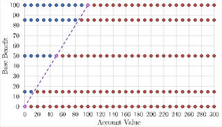
Figure 4.3: The grids used in the Full Regression method and in the Regression by Lines for a GMWB with $T_{2}=10$ and annual withdrawals. In the first picture, violet points are used in both the two regions. In the second picture, for each $B$ level, the gray points border the different sectors and they are shared. The degree of the polynomials for this last case is $4$.

Optimal surrender

This case concerns GMWB-YD products. In their articles, Yang and Dai suppose the PH to be entitled to surrender when optimal.

In this case we suppose that at each event time $t_{i}\in\left\{t_{1},\dots,t_{N}\right\}$ the PH can withdraw the contract amount, or fully surrender. As we did before, similarity reduction let us fix the value of $G$. We denote $\mathcal{V}\left(A,t\right)$ the expected value at time $t$ of a generic policy whose state parameter is $A$ (similarity reduction let us use only $A$ as variable) :

$$\mathcal{V}\left(A,t\right)=\mathbb{E}\left[V_{s}\left(A,t\right)\right].$$

So, we suppose that the PH surrenders at time $t_{i^{*}}$ if

$$\left(1-\kappa\right)\max\left(A_{t_{i^{*}}^{-}}-G,0\right)\geq\mathcal{V}\left(\max\left(A_{t_{i^{*}}^{-}}-G,0\right),t\right).$$

The expected value $\mathcal{V}$ can be calculated with a standard Longstaff-Schwartz approach:

1. Simulate $N$ random scenarios and price the policy into these scenarios assuming that the PH follows a static approach.

2. For $t_{i}=t_{N}$ to $t_{i}=t_{1}$:

   1. Approximate the function $\mathcal{V}\left(A,t_{i}\right)$ using the least squares projection into a space of functions (usually polynomials).

   2. For each scenario evaluate if $t_{i}$ is the good stopping time.

3. Use at time $T_{1}$ similarity reduction to include account value reset.

4. Calculate the average of the initial value $V_{s}\left(P,0\right)$ for all the scenarios to approximate $\mathcal{V}\left(P,0\right)$.

4.2 Standard Monte Carlo Method

The Monte Carlo method is very similar to the Hybrid Monte Carlo one. The only difference is the way we produce the random scenarios. The projection phase is the same as Hybrid Monte Carlo one.

4.2.1 Scenario generation

We distinguish two cases for the two models.

The Heston Model

The generation of the scenarios (underlying and volatility) in this case has been done using a third order scheme described in Alfonsi [1].

The Black-Scholes Hull-White Model

The generation of the scenarios (underlying and interest rate) in this case has been done using an exact scheme described in Ostrovski [21], with a few changes in order to incorporate the correlation between underlying and interest rate.

4.3 PDE Hybrid Method

The Hybrid PDE approach is different from the previous ones. In fact it’s a PDE pricing method and it’s based on Briani et al. [6], [7] both for Heston and Hull-White case. Using a tree to diffuse volatility or interest rate, we freeze these values between two tree-levels and we solve a Black Scholes PDE for each node of the tree, using as initial data a weighted mix of the data of the upcoming nodes.

We can resume the pricing methods in three features: model, algorithm structure and pricing.

We start describing the model between the event times.

4.3.1 The Heston Model

Starting from the model for the found $S_{t}$ in (3.1), we call $\bar{\rho}=\sqrt{1-\rho^{2}}$ and we write $Z_{t}^{A}=\rho Z_{t}^{v}+\bar{\rho}\bar{Z}_{t}^{A}$, where $\bar{Z}^{A}$ is a Brownian motion uncorrelated with $Z^{v}$. Then,

$$\begin{cases}dA_{t}=\left(r-\alpha_{tot}\right)A_{t}dt+\sqrt{v_{t}}A_{t}\left(\rho dZ_{t}^{v}+\bar{\rho}d\bar{Z}_{t}^{A}\right)&v_{0}=\bar{v}_{0},\\ dv_{t}=k\left(\theta-v_{t}\right)dt+\omega\sqrt{v_{t}}dZ_{t}^{V}&A_{0}=\bar{A}_{0},\end{cases}\ \ \ d\left\langle\bar{Z}_{t}^{A},Z_{t}^{v}\right\rangle=0,$$

covering the behavior of $A_{t}$ between two event times, we define the process

$$Y_{t}^{E}=\ln\left(A_{t}\right)-\frac{\rho}{\omega}v_{t},\ Y_{0}^{E}=\ln\left(A_{0}\right)-\frac{\rho}{\omega}v_{0}$$

Then,

$$A_{t}=\exp\left(Y_{t}^{E}+\frac{\rho}{\omega}v_{t}\right)$$ (4.1)

and

$$dY_{t}^{E}=\left(r-\alpha_{tot}-\frac{v_{t}}{2}-\frac{\rho}{\omega}k\left(\theta-v_{t}\right)\right)dt+\bar{\rho}\sqrt{v_{t}}d\bar{Z}_{t}^{A}.$$

This process $Y^{E}$ is important because it’s a process uncorrelated with the volatility process $v$, and we introduce it as in [6]. We are going to use it to define a PDE to be solved along the tree.

We define $\hat{\mathcal{V}}^{He}\left(t,Y_{t}^{E}\right)=\mathcal{V}\left(t,A_{t}\right)$.

If, in a small time lag $\left[\tau,\tau+\Delta\tau\right]$, we approximate the process $Y_{t}^{E}$ by the process $\bar{Y}_{t}^{E}$ whose dynamics is given by

$$d\bar{Y}_{t}^{E}=\left(r-\alpha_{tot}-\frac{v_{\tau}}{2}-\frac{\rho}{\omega}k\left(\theta-v_{\tau}\right)\right)dt+\bar{\rho}\sqrt{v_{\tau}}d\bar{Z}_{t}^{A}.$$

Then, $\hat{\mathcal{V}}^{He}\left(t,\bar{Y}_{t}^{E}\right)$ verifies the following PDE

$$\frac{\partial\hat{\mathcal{V}}^{He}}{\partial t}+\left(r-\alpha_{tot}-\frac{v_{\tau}}{2}-\frac{\rho}{\omega}k\left(\theta-v_{\tau}\right)\right)\frac{\partial\hat{\mathcal{V}}^{He}}{\partial\bar{Y}_{t}^{E}}+\frac{\bar{\rho}^{2}v_{\tau}}{2}\frac{\partial^{2}\hat{\mathcal{V}}^{He}}{\partial^{2}\bar{Y}_{t}^{E}}-r\hat{\mathcal{V}}^{He}=0.$$ (4.2)

4.3.2 The Black-Scholes Hull-White Model

Starting from the model for the found $S_{t}$ in (3.2), we call $\bar{\rho}=\sqrt{1-\rho^{2}}$ and we write $Z_{t}^{A}=\rho Z_{t}^{r}+\bar{\rho}\bar{Z}_{t}^{A}$, where $\bar{Z}^{A}$ is a Brownian motion uncorrelated with $Z^{r}$. Then,

$$\begin{cases}dA_{t}=A_{t}\left(r-\alpha_{tot}\right)dt+\sigma A_{t}\left(\rho dZ_{t}^{r}+\bar{\rho}d\bar{Z}_{t}^{A}\right)&A_{0}=\bar{A}_{0},\\ dX_{t}=-kX_{t}dt+dZ_{t}^{r}&X_{0}=0,\\ r_{t}=\omega X_{t}+\beta\left(t\right),\end{cases}\ \ \ d\left\langle\bar{Z}_{t}^{A},Z_{t}^{r}\right\rangle=0.$$

We define the process

$$Y_{t}^{U}=\ln\left(A_{t}\right)-\rho\sigma X_{t},\ Y_{0}^{U}=\ln\left(A_{0}\right)$$

Then,

$$A_{t}=\exp\left(Y_{t}+\rho\sigma X_{t}\right)$$ (4.3)

and

$$dY_{t}^{U}=\left(r_{t}-\alpha_{tot}-\frac{\sigma^{2}}{2}+\sigma\rho kX_{t}\right)dt+\sigma\bar{\rho}d\bar{Z}_{t}^{A}.$$

This process $Y^{U}$ is important because it’s a process uncorrelated with the mean-reverting process $X$, and we introduce it as in [6]. We are going to use it to define a PDE to be solved along the tree.

We define $\hat{\mathcal{V}}^{HW}\left(t,Y_{t}^{U}\right)=\mathcal{V}\left(t,A_{t}\right)$. If, in a small time lag $\left[\tau,\tau+\Delta\tau\right]$, we approximate the process $Y_{t}^{U}$ by the process $\bar{Y}_{t}^{U}$ whose dynamics is given by

$$d\bar{Y}_{t}^{U}=\left(r_{\tau}-\alpha_{tot}-\frac{\sigma^{2}}{2}+\sigma\rho kX_{\tau}\right)dt+\sigma\bar{\rho}dZ_{t},$$

and the interest rate process by $r_{\tau}$, then, $\hat{\mathcal{V}}^{HW}\left(t,\bar{Y}_{t}^{U}\right)$ verifies the following PDE

$$\frac{\partial\hat{\mathcal{V}}^{HW}}{\partial t}+\left(r_{\tau}-\alpha_{tot}-\frac{\sigma^{2}}{2}+\sigma\rho kX_{\tau}\right)\frac{\partial\hat{\mathcal{V}}^{HW}}{\partial\bar{Y}_{t}^{U}}+\frac{\bar{\rho}^{2}\sigma^{2}}{2}\frac{\partial^{2}\hat{\mathcal{V}}^{HW}}{\partial^{2}\bar{Y}_{t}^{U}}-r_{\tau}\hat{\mathcal{V}}^{HW}=0.$$ (4.4)

4.3.3 Algorithm structure

The structures for this algorithm consist in a tree and a PDE solver. As described in Briani et al. [6], [7], we use a tree to diffuse the volatility (or the interest rate) along the life of the product, and we solve backward a 1D PDE freezing at each node of the tree the volatility (or the interest rate). The tree is built according to Section 4.1.1 (quadrinomial tree, matching the first three moments of the process), and the PDE is solved with a finite difference approach. We have to solve the PDE between event times, and at each event time we apply the changes to the states to reproduce the effects of the events.

We remark that we solve the PDE doing a single time step that requires only a linear complexity because we have to solve a linear system with tridiagonal matrix. The computational cost is low as observed in [6] and [7]. We observe that $X_{t}$ and $V_{t}$ processes are mean reverting. Thanks to the way the trees are built, there are many nodes in the trees that cannot be visited by the approximating Markov chain. Therefore their probability $p_{n,j}$ to be visited is worth $0$ and they have no impact on the values at the root of the tree. There is no reason to do any operation for those nodes. So, to save time, we do the standard step (mix up the vectors according to the transition probabilities and solve backward a PDE) only for those nodes having $p_{n,j}>0$. This curtailing technique reduces the computational time, and the convergence of the method is preserved. A similar approach is used in [2].

4.3.4 Pricing

We distinguish 3 cases.

Static case

This case is common to both GMWB-CF and GMWB-YD products. The problem dimension is 2: about GMWB-CF, at each event time the value of the the base benefit $B_{t_{i}}$ is equal to $P-G\cdot i$ and thus it’s not a problem variable; about GMWB-YD similarity reduction reduce problem dimension to 2.

For each node of the tree we have to solve one PDE using the mixture of the the data of the upcoming nodes: the mixture is done according to transition probabilities. The PDE to be solved are those in (4.2) and (4.4) where $\left[\tau,\tau+\Delta\tau\right]$ denotes the time lag between two tree nodes.

The variables $\bar{r}$, $\bar{X}$ and $\bar{v}$ will denote the frozen values of $r_{t}$, $X_{t}$ and $v_{t}$ using the data of the actual node. We used a finite differences approach using equally spaced nodes for $Y_{t}$ processes. To reduce the run time, we do this only for most relevant nodes: this cutting technique dramatically reduced calculation times without compromising the quality of results. Then, using the inverse transformations (4.1) and (4.3), we apply the event times actions in (2.3) or equivalently (2.4).

Optimal Withdrawal

This case is about GMWB-CF products. This is the hardest to be treated because the problem dimension is 3. We solve the same PDE as in Static case, but this time we have to solve them for different values of $B_{t}$ and chose the best withdrawal $W_{t}$ at each event time. Numerical test showed that it’s enough to search the best withdrawal between multiples of $G$ equal or smaller than the base benefit. Then we decided to solve the problem for all $B_{t}$ values of which are multiples of $G$ and are smaller than the initial premium $P$: $B=0$, $B=G$, $B_{t}=2G$, $\dots$$B=nG=P$. Then, we solve $n$ 2-dimensional problems rather then one 3-dimensional problem. This approach is similar to “Regression by Lines” defined for MC methods.

Best withdrawal search is performed searching among permissible withdrawals which are multiples of $G$: $W=0,$ $W=G,$$\dots$$W=mG=B$. The estimate of $\mathcal{V}\left(A,B\right)$ for those values of $A$ that aren’t on the grid, is done using splines.

In Figure 4.4 we can see a scheme that represents what happens for a product with $G=20$: for example, a $5$ years maturity GM with annual withdrawal rate and $P=100$ ($G=20$). Nodes are exponentially distributed (uniformly for $Y$ process) and for each $B$ value, we add a node that represents $A=0$ (blue nodes). For each node, first we mix the data vectors of the upcoming nodes according to transition probabilities. Then we solve a PDE backward starting from the mixture of the data. Then we apply withdrawal step: for each node we consider admissible withdrawals of the type $W=kG$ and we chose the value that maximize PH’s benefit: cash flow plus policy value. This research is shown in the Figure (see yellow nodes that corresponds to possible withdrawals).

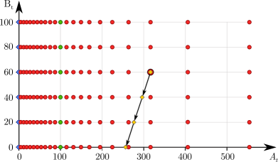
Figure 4.4: The scheme for PDE optimal withdrawal for a given node.

Optimal surrender

This case is about GMWB-YD products. It’s much more simpler than optimal withdrawal. In fact, the PH can only chose between withdrawal at the contract rate and fully surrender.

Withdrawal step at event time $t_{i}$ consists into replacing $\mathcal{V}\left(A,t_{i}\right)$ by

$$\max\left[G+\mathcal{V}\left(\max\left(A-G,0\right),t_{i}\right);G+\left(1-\kappa\right)\left(A-G\right)\right].$$

4.4 PDE ADI Method

We propose a PDE pricing method with alternative direction implicit scheme which has been already successfully used for European financial product (see [14]) and for an insurance GLWB product (see [13]). This method permits to treat the Heston model and the BS HW model. This method is fast and accurate. Moreover it is easy to take into account the similarity reduction and the optimal behavior. For this method, we followed the same principles of HPDE method about taking in account the event times.

The PDEs to be solved in the two models are

$$\mathcal{V}_{t}^{He}+\frac{VA^{2}}{2}\mathcal{V}_{AA}^{He}+\frac{\omega^{2}V}{2}\mathcal{V}_{VV}^{He}+\left(r-\alpha_{tot}\right)A\mathcal{V}_{A}^{He}+\rho\omega AV\mathcal{V}_{AV}^{He}+k\left(\theta-V\right)\mathcal{V}_{V}^{He}-r\mathcal{V}^{He}=0\$$

$$\mathcal{V}_{t}^{HW}+\frac{\sigma^{2}A^{2}}{2}\mathcal{V}_{AA}^{HW}+\frac{\omega^{2}}{2}\mathcal{V}_{rr}^{HW}+\left(r-\alpha_{tot}\right)A\mathcal{V}_{A}^{HW}+\rho\omega A\sigma\mathcal{V}_{Ar}^{HW}+k\left(\theta_{t}-r\right)\mathcal{V}_{r}^{HW}-r\mathcal{V}^{HW}=0\$$

There are multiple numerical parameters which have to be carefully chosen. We have to choose the grids for the benefit base, the account value, the rate in the BS HW model and the volatility in the Heston model. We have chosen to use the meshes described in [14] with the parameters

$$A_{left}=0.8S_{0}\quad A_{right}=1.2S_{0}\quad A_{max}=1000\cdot T2\cdot S_{0}\quad\text{ and }d_{1}=S_{0}/20,$$

for the mesh of variable $A$,

$$R_{\max}=0.8,\quad c=R_{0}\quad\text{ and }d_{2}=R_{\max}/400$$

for the mesh of variable $r$ in the BS HW model, and

$$V_{\max}=MIN(MAX(100V_{0},1),5)\quad\text{ and }d_{3}=V_{\max}/500.$$

for the mesh of variable $V$ in the Heston model. Some grid are uniform or based on hyperbolic transformation. Moreover the boundary conditions are completely unknown, and an asymptotic study would be necessary to chose them. We have chosen homogeneous Neumann boundary conditions, and we have chosen very large grids to avoid that this choice impacts the results. We have only used the Douglas scheme, but other schemes are possible to have better order of convergence in time. Thus many possibilities are possible to improve the ADI scheme, but the easier is already enough to obtain good results.

5 Numerical Results

In this Section we compare the numerical methods used in Section 4: Hybrid Monte Carlo (HMC), Standard Monte Carlo (SMC), Hybrid PDE (HPDE), and ADI PDE (APDE). In particular we compare pricing and Greeks computation in Static Case and Dynamic Case for both the two product types.

We chose the parameters of the methods according to 4 configurations (A, B, C, D), with an increasing number of steps and so that the calculation time for the various methods in each configuration were close. The 4 configurations are in Table 1 and in Table 2 with the notation (time steps per year $\times$ space steps $\times$ vol steps) for the ADI PDE method, (time steps per year $\times$ space steps ) for the Hybrid PDE method and (time steps per year $\times$ number of simulations) for the MC ones. In Monte Carlo for Dynamic case, we also add the degree of the approximating polynomial. These values have been chosen to achieve approximately these run times using an ordinary computer: $\left(A\right)$ 30 s, $\left(B\right)$ 120 s, $\left(C\right)$ 480 s, $\left(D\right)$ 1920 s. To reduce the run time we do the secant iterations using an increasing number of time steps for all the methods: the values in Table 1 and 2 are those used for the last 3 iterations.

We use the Standard MC both as a pricing method, both as a benchmark (BM). About the benchmark, in the Static case we used $10^{8}$ independent runs. In the Dynamic case we used $10^{6}$ independent runs; in each sub runs the expected value has been approximated by a $4^{th}$ degree polynomial.

The search for the fair $\alpha_{g}$ value has been driven by the secant method. The initial values for this method were $\alpha_{g}=0$ bp and $\alpha_{g}=200$ bp.

To achieve Delta calculation in Monte Carlo methods we used a $1\permil$ shock in Static case and $1\%$ in Dynamic case.

	BS HW Static				Heston Static
	HMC	SMC	HPDE	APDE	HMC	SMC	HPDE	APDE
A	$4\negthinspace\times\negthinspace 9.2\negthinspace\cdot\negthinspace 10^{5}$	$1\negthinspace\times\negthinspace 1.7\negthinspace\cdot\negthinspace 10^{6}$	$260\negthinspace\times\negthinspace 250$	$25\negthinspace\times\negthinspace 250\!\times 505$	$4\negthinspace\times\negthinspace 5.8\negthinspace\cdot\negthinspace 10^{5}$	$4\negthinspace\times\negthinspace 5.2\negthinspace\cdot\negthinspace 10^{5}$	$270\negthinspace\times\negthinspace 250$	$25\negthinspace\times\negthinspace 250\!\times 505$
B	$8\negthinspace\times\negthinspace 1.8\negthinspace\cdot\negthinspace 10^{6}$	$1\negthinspace\times\negthinspace 5.7\negthinspace\cdot\negthinspace 10^{6}$	$420\negthinspace\times\negthinspace 500$	$40\negthinspace\times\negthinspace 400\!\times 85$	$8\negthinspace\times\negthinspace 1.2\negthinspace\cdot\negthinspace 10^{6}$	$8\negthinspace\times\negthinspace 1.2\negthinspace\cdot\negthinspace 10^{6}$	$520\negthinspace\times\negthinspace 500$	$40\negthinspace\times\negthinspace 400\!\times 80$
C	$12\negthinspace\times\negthinspace 6.3\negthinspace\cdot\negthinspace 10^{6}$	$1\negthinspace\times\negthinspace 2.9\negthinspace\cdot\negthinspace 10^{7}$	$780\negthinspace\times\negthinspace 1000$	$60\negthinspace\times\negthinspace 620\!\times 125$	$12\negthinspace\times\negthinspace 3.9\negthinspace\cdot\negthinspace 10^{6}$	$12\negthinspace\times\negthinspace 3.4\negthinspace\cdot\negthinspace 10^{6}$	$850\negthinspace\times\negthinspace 1000$	$60\negthinspace\times\negthinspace 620\!\times 120$
D	$16\negthinspace\times\negthinspace 1.9\negthinspace\cdot\negthinspace 10^{7}$	$1\negthinspace\times\negthinspace 1.2\negthinspace\cdot\negthinspace 10^{8}$	$1200\negthinspace\times\negthinspace 2000$	$100\negthinspace\times\negthinspace 1000\!\times 215$	$16\negthinspace\times\negthinspace 1.2\negthinspace\cdot\negthinspace 10^{7}$	$16\negthinspace\times\negthinspace 1.1\negthinspace\cdot\negthinspace 10^{7}$	$1400\negthinspace\times\negthinspace 2000$	$100\negthinspace\times\negthinspace 1000\!\times 200$

	BS HW Dynamic				Heston Dynamic
	HMC	SMC	HPDE	APDE	HMC	SMC	HPDE	APDE
A	$4\negthinspace\times\negthinspace 6.0\!\cdot\!10^{4}\negthinspace\times\negthinspace 1$	$1\negthinspace\times\negthinspace 6.5\!\cdot\!10^{4}\negthinspace\times\negthinspace 1$	$70\negthinspace\times\negthinspace 250$	$8\negthinspace\times\negthinspace 95\!\times 30$	$4\negthinspace\times\negthinspace 5.1\!\cdot\!10^{4}\negthinspace\times\negthinspace 1$	$4\negthinspace\times\negthinspace 5.5\!\cdot\!10^{4}\negthinspace\times\negthinspace 1$	$88\negthinspace\times\negthinspace 250$	$10\negthinspace\times\negthinspace 125\!\times 25$
B	$8\negthinspace\times\negthinspace 8.7\!\cdot\!10^{4}\negthinspace\times\negthinspace 2$	$1\negthinspace\times\negthinspace 9.5\!\cdot\!10^{4}\negthinspace\times\negthinspace 2$	$160\negthinspace\times\negthinspace 500$	$14\negthinspace\times\negthinspace 150\!\times 48$	$8\negthinspace\times\negthinspace 1.2\!\cdot\!10^{4}\negthinspace\times\negthinspace 2$	$8\negthinspace\times\negthinspace 1.3\!\cdot\!10^{4}\negthinspace\times\negthinspace 2$	$160\negthinspace\times\negthinspace 500$	$15\negthinspace\times\negthinspace 200\!\times 40$
C	$12\negthinspace\times\negthinspace 1.8\!\cdot\!10^{5}\negthinspace\times\negthinspace 3$	$1\negthinspace\times\negthinspace 1.9\!\cdot\!10^{5}\negthinspace\times\negthinspace 3$	$270\negthinspace\times\negthinspace 1000$	$22\negthinspace\times\negthinspace 250\!\times 75$	$12\negthinspace\times\negthinspace 2.3\!\cdot\!10^{5}\negthinspace\times\negthinspace 3$	$12\negthinspace\times\negthinspace 2.5\!\cdot\!10^{5}\negthinspace\times\negthinspace 3$	$266\negthinspace\times\negthinspace 1000$	$25\negthinspace\times\negthinspace 320\!\times 60$
D	$16\negthinspace\times\negthinspace 3.5\!\cdot\!10^{5}\negthinspace\times\negthinspace 4$	$1\negthinspace\times\negthinspace 3.5\!\cdot\!10^{5}\negthinspace\times\negthinspace 4$	$360\negthinspace\times\negthinspace 2000$	$35\negthinspace\times\negthinspace 400\!\times 120$	$16\negthinspace\times\negthinspace 4.2\!\cdot\!10^{5}\negthinspace\times\negthinspace 4$	$16\negthinspace\times\negthinspace 5.0\!\cdot\!10^{5}\negthinspace\times\negthinspace 4$	$350\negthinspace\times\negthinspace 2000$	$40\negthinspace\times\negthinspace 500\!\times 90$

Table 1: Configuration parameters for the BS HW model and for the Heston model, Static and Dynamic for the GMWB-CF product with $T_{2}=10$ and $WF=1$.

	BS HW Static				Heston Static
	HMC	SMC	HPDE	APDE	HMC	SMC	HPDE	APDE
A	$4\negthinspace\times\negthinspace 3.2\negthinspace\cdot\negthinspace 10^{5}$	$1\negthinspace\times\negthinspace 6.0\negthinspace\cdot\negthinspace 10^{5}$	$130\negthinspace\times\negthinspace 250$	$10\negthinspace\times\negthinspace 245\!\times 50$	$4\negthinspace\times\negthinspace 2.3\negthinspace\cdot\negthinspace 10^{5}$	$4\negthinspace\times\negthinspace 2.0\negthinspace\cdot\negthinspace 10^{5}$	$120\negthinspace\times\negthinspace 250$	$10\negthinspace\times\negthinspace 250\!\times 50$
B	$8\negthinspace\times\negthinspace 6.4\negthinspace\cdot\negthinspace 10^{5}$	$1\negthinspace\times\negthinspace 2.3\negthinspace\cdot\negthinspace 10^{6}$	$215\negthinspace\times\negthinspace 500$	$15\negthinspace\times\negthinspace 375\!\times 80$	$8\negthinspace\times\negthinspace 4.6\negthinspace\cdot\negthinspace 10^{5}$	$8\negthinspace\times\negthinspace 3.8\negthinspace\cdot\negthinspace 10^{5}$	$220\negthinspace\times\negthinspace 500$	$15\negthinspace\times\negthinspace 380\!\times 80$
C	$12\negthinspace\times\negthinspace 2.2\negthinspace\cdot\negthinspace 10^{6}$	$1\negthinspace\times\negthinspace 1.2\negthinspace\cdot\negthinspace 10^{7}$	$415\negthinspace\times\negthinspace 1000$	$35\negthinspace\times\negthinspace 520\!\times 110$	$12\negthinspace\times\negthinspace 1.6\negthinspace\cdot\negthinspace 10^{6}$	$12\negthinspace\times\negthinspace 1.3\negthinspace\cdot\negthinspace 10^{6}$	$425\negthinspace\times\negthinspace 1000$	$36\negthinspace\times\negthinspace 530\!\times 110$
D	$16\negthinspace\times\negthinspace 6.8\negthinspace\cdot\negthinspace 10^{6}$	$1\negthinspace\times\negthinspace 4.5\negthinspace\cdot\negthinspace 10^{7}$	$480\negthinspace\times\negthinspace 2000$	$55\negthinspace\times\negthinspace 880\!\times 180$	$16\negthinspace\times\negthinspace 4.8\negthinspace\cdot\negthinspace 10^{6}$	$16\negthinspace\times\negthinspace 4.0\negthinspace\cdot\negthinspace 10^{6}$	$480\negthinspace\times\negthinspace 2000$	$55\negthinspace\times\negthinspace 890\!\times 180$

	BS HW Dynamic				Heston Dynamic
	HMC	SMC	HPDE	APDE	HMC	SMC	HPDE	APDE
A	$4\negthinspace\times\negthinspace 6.8\negthinspace\cdot\negthinspace 10^{4}\!\times 1$	$1\negthinspace\times\negthinspace 8.1\negthinspace\cdot\negthinspace 10^{4}\!\times 1$	$130\negthinspace\times\negthinspace 250$	$10\negthinspace\times\negthinspace 245\!\times 50$	$4\negthinspace\times\negthinspace 5.5\negthinspace\cdot\negthinspace 10^{4}\!\times 2$	$4\negthinspace\times\negthinspace 5.8\negthinspace\cdot\negthinspace 10^{4}\!\times 2$	$120\negthinspace\times\negthinspace 250$	$10\negthinspace\times\negthinspace 250\!\times 50$
B	$8\negthinspace\times\negthinspace 2.5\negthinspace\cdot\negthinspace 10^{5}\!\times 2$	$1\negthinspace\times\negthinspace 3.4\negthinspace\cdot\negthinspace 10^{5}\!\times 2$	$215\negthinspace\times\negthinspace 500$	$15\negthinspace\times\negthinspace 375\!\times 80$	$8\negthinspace\times\negthinspace 2.2\negthinspace\cdot\negthinspace 10^{5}\!\times 3$	$8\negthinspace\times\negthinspace 2.0\negthinspace\cdot\negthinspace 10^{5}\!\times 3$	$220\negthinspace\times\negthinspace 500$	$15\negthinspace\times\negthinspace 380\!\times 80$
C	$12\negthinspace\times\negthinspace 6.9\negthinspace\cdot\negthinspace 10^{5}\!\times 3$	$1\negthinspace\times\negthinspace 9.7\negthinspace\cdot\negthinspace 10^{5}\!\times 3$	$415\negthinspace\times\negthinspace 1000$	$35\negthinspace\times\negthinspace 520\!\times 110$	$12\negthinspace\times\negthinspace 5.9\negthinspace\cdot\negthinspace 10^{5}\!\times 4$	$12\negthinspace\times\negthinspace 5.6\negthinspace\cdot\negthinspace 10^{5}\!\times 4$	$425\negthinspace\times\negthinspace 1000$	$36\negthinspace\times\negthinspace 530\!\times 110$
D	$16\negthinspace\times\negthinspace 1.8\negthinspace\cdot\negthinspace 10^{6}\!\times 4$	$1\negthinspace\times\negthinspace 1.8\negthinspace\cdot\negthinspace 10^{6}\!\times 4$	$480\negthinspace\times\negthinspace 2000$	$55\negthinspace\times\negthinspace 880\!\times 180$	$16\negthinspace\times\negthinspace 1.5\negthinspace\cdot\negthinspace 10^{6}\!\times 5$	$16\negthinspace\times\negthinspace 1.5\negthinspace\cdot\negthinspace 10^{6}\!\times 5$	$480\negthinspace\times\negthinspace 2000$	$55\negthinspace\times\negthinspace 890\!\times 180$

Table 2: Configuration parameters for the BS HW model and for the Heston model, Static and Dynamic for the GMWB-YD product with $\left(T_{1},T_{2}\right)=\left(10,25\right)$

5.1 Static Withdrawal for GMWB-CF

In the Static Withdrawal case we suppose the PH to withdrawal exactly at the guaranteed rate.

The Static Tests 1 and 2 are inspired by [9]: in their article, Chen and Forsyth price a GMWB contract according to an optimal withdrawal framework, under the Black Scholes model. First we priced their product for different maturities and withdrawal rates, assuming Static withdrawals in Black and Scholes model to get a reference price in this model; we got the $\alpha$ value using both a standard Monte Carlo method and a standard PDE method. As we easily got the correct values for the simple Black-Scholes model, then we add stochastic interest rate and stochastic volatility. Model parameters are available in Table 4, and the values of $\alpha_{g}$ that we got in the Black-Scholes case are given in Table 4.

5.1.1 Test 1: Static GMWB-CF in the Black-Scholes Hull-White Model

In this test we want to price a GMWB-CF product according to BS HW model. We use the same corresponding parameters as in the Black Scholes model. Model parameters are shown in Table 6. Results are available in Table 6.

All the four methods behaved well and in the configuration D they gave results consistent with the benchmark. HPDE proved to be the best: all of its configurations gave results consistent with the benchmark. Then APDE and SMC, and HMC gave good results too. SMC performed a little better than HMC: the first method simulates the underlying value and the interest rate exactly and so it is enough to simulate the values at each event time. HMC matches the first three moments of the BS HW $r$ process, but it doesn’t reproduce exactly its law: therefore it is right to increase the number of steps per year. So, for a given run time, we can simulate less scenarios in HMC than SMC: effectively, the confidence interval of HMC is larger than SMC one. Moreover, SMC over performed the benchmark when using configuration D. The two PDE methods returned stable results, and they often converged in a monotone way.

With regard to the numerical results, we observe that the $\alpha_{g}$ values decrease with increasing maturity, just as in the Black-Scholes case, and increase a little, with increasing withdrawal frequency.

5.1.2 Test 2: Static GMWB-CF in the Heston Model

In this test we want to price a GMWB-CF product according to the Heston model. Model parameters are shown in the Table 8. Results are shown in Table 8.

In this Test, MC methods had more difficulties; all the values of PDE methods were close to the benchmark, while some values from MC methods were less accurate, but compatibles with the benchmark (the value of BM is inside the MC confidence interval). If we compare the two MC approaches, in this case they are equivalent: HMC proved to be faster than SMC when using few time steps (we could exploit $+11\%$ simulations in configuration A), while SMC proved to be slightly faster in high time steps simulations, because of more time needed to build the volatility tree ($-8\%$ simulations in configuration D). HPDE shows to be very stable (case $T_{2}=10$, $WF=2$, $\alpha_{g}$ didn’t change through configurations B-D), APDE behaved well to (often monotone convergence).

With regard to the numerical results, we observe that the $\alpha_{g}$ values decrease with increasing maturity, just as in the Black-Scholes case, and increase a little, with increasing withdrawal frequency.

5.1.3 Test 3: Hedging for Static GMWB-CF

To reduce financial risks, insurance companies have to hedge the sold VA: to accomplish this target they must calculate the Greeks of products.

In this test we want to show how the different methods can be used to calculate the main Greeks. This can be done through finite differences for small shocks on the variables. In general, the PDE methods are ahead w.r.t. MC methods: the price is computed through finite differences and so the price under shock is already computed. For MC methods this is quite harder because the pricing has to be repeated changing the inputs.

To start, we calculate the underlying greek Delta, for the products of Test 1 and Test 2. As in this case we don’t want to compute the fair fee $\alpha_{g}$, we fix it arbitrarily: see Table 10 and Table 12. The values chosen are such as to cover the costs of the insurer, and may be plausible on a real case. Results are available in Table 10 (all values in Table must be multiplied by $10^{-4}$).

In this Test, we got very accurate results with all method. Anyway, HPDE and APDE proved to be the best: they both gave stable and accurate results; in this Test, the two PDE methods were equivalent. We remark that despite fair fee changes a lot when changing the maturity of the policy, the value of Delta changes much less. Delta calculation proved to be slightly harder in the Heston model case than in the BS HW model case: see confidence intervals.

Expiry Time $T$	5, 10, 20 Years		GMW $G$	$100.0/(T\cdot WF)$
Withdrawal Frequency $WF$	1 or 2 per Year		Initial Premium	$100.0$
Initial account value $A_{0}$	$100.0$		$S_{0}$	$100.0$
Initial base b. value $B_{0}$	$100.0$		$r$	$0.05$
Withdrawal penalty $\kappa$	$0.10$		$\sigma$	$0.20$
Management fees $\alpha_{m}$	$0$

Table 3: Parameters used by Chen and Forsyth in [9].

$T_{2}$	$WF=1$		$WF=2$
	PDE	MC	PDE	MC
$5$	$235.24$	$235.11\pm 0.42$	$243.96$	$243.80\pm 0.42$
$10$	$92.41$	$92.28\pm 0.30$	$94.62$	$94.84\pm 0.30$
$20$	$27.64$	$27.79\pm 0.24$	$28.09$	$28.39\pm 0.24$

Table 4: Fair bp values of $\alpha_{g}$ in Black Scholes model, for Static GMWB-CF with the same parameters as in [9].

$S_{0}$	$r$	$curve$	$k$	$\omega$	$\rho$	$\sigma$
$100$	$0.05$	$flat$	$1.0$	$0.2$	$-0.5$	$0.20$

Table 5: The model parameters about Test 1

$T_{2}$ $WF=1$ $WF=2$ HMC SMC HPDE APDE BM HMC SMC HPDE APDE BM $5$ A $191.05\pm 0.83$ $190.81\pm 0.66$ $191.03$ $191.16$ $191.34$ $196.87\pm 0.88$ $196.79\pm 0.94$ $196.39$ $196.50$ $196.77$ B $191.79\pm 0.59$ $191.25\pm 0.33$ $191.18$ $191.58$ $196.88\pm 0.62$ $197.02\pm 0.47$ $196.55$ $196.60$ C $191.34\pm 0.32$ $191.26\pm 0.15$ $191.25$ $191.47$ $\pm 0.11$ $196.72\pm 0.34$ $196.64\pm 0.21$ $196.62$ $196.88$ $\pm 0.11$ D $191.20\pm 0.18$ $191.25\pm 0.07$ $191.27$ 191.38 $196.55\pm 0.19$ $196.67\pm 0.10$ $196.65$ $196.68$ $10$ A $79.71\pm 0.84$ $79.26\pm 0.66$ $79.41$ $79.33$ $79.44$ $81.38\pm 0.88$ $81.13\pm 0.94$ $80.98$ $81.32$ $80.97$ B $79.80\pm 0.60$ $79.43\pm 0.33$ $79.39$ $79.41$ $80.95\pm 0.63$ $81.42\pm 0.47$ $80.98$ $80.64$ C $79.61\pm 0.32$ $79.56\pm 0.15$ $79.39$ $79.41$ $\pm 0.08$ $81.12\pm 0.34$ $81.12\pm 0.21$ $80.98$ $81.01$ $\pm 0.08$ D $79.35\pm 0.18$ $79.44\pm 0.07$ $79.38$ $79.40$ $80.90\pm 0.19$ $80.98\pm 0.10$ $80.99$ $81.01$ $20$ A $26.33\pm 0.98$ $25.04\pm 0.77$ $24.90$ $24.90$ $24.81$ $25.04\pm 1.07$ $25.72\pm 1.06$ $25.27$ $25.20$ $25.16$ B $25.92\pm 0.69$ $25.23\pm 0.39$ $24.86$ $24.67$ $25.91\pm 0.75$ $25.59\pm 0.54$ $25.23$ $25.16$ C $25.16\pm 0.37$ $24.91\pm 0.17$ $24.84$ $24.81$ $\pm 0.07$ $25.16\pm 0.41$ $25.35\pm 0.24$ $25.21$ $25.18$ $\pm 0.07$ D $24.99\pm 0.21$ $24.81\pm 0.09$ $24.84$ $24.82$ $25.40\pm 0.23$ $25.13\pm 0.12$ $25.20$ $25.18$

HMC SMC HPDE APDE A $31$ s $30$ s $30$ s $30$ s B $121$ s $121$ s $120$ s $118$ s C $482$ s $484$ s $464$ s $481$ s D $1920$ s $1899$ s $1893$ s $1909$ s

Table 6: Test 1. In the first Table, the fair fee $\alpha_{g}$ in bps for the Black-Scholes Hull-White model, with annual or six-monthly withdrawal. In the second Table the run times for the case $WF=1$, $T_{2}=10$. Finally, the plot of relative error (w.r.t. BM value) for the four methods in the same case of run-times Table. The parameters used for this test are available in Table 4 and in Table 6.

$S_{0}$	$v_{0}$	$\theta$	$k$	$\omega$	$\rho$	$r$
$100$	$0.20^{2}$	$0.20^{2}$	$1.0$	$0.2$	$-0.5$	$0.05$

Table 7: The model parameters about Test 2.

$T_{2}$ $WF=1$ $WF=2$ HMC SMC HPDE APDE BM HMC SMC HPDE APDE BM $5$ A $232.30\pm 0.97$ $232.83\pm 1.03$ $231.20$ $231.62$ $231.38$ $239.82\pm 1.00$ $240.88\pm 1.05$ $239.34$ $239.51$ $239.54$ B $231.72\pm 0.68$ $231.73\pm 0.75$ $231.37$ $231.55$ $240.41\pm 0.71$ $239.76\pm 0.77$ $239.52$ $239.38$ C $231.39\pm 0.37$ $231.56\pm 0.41$ $231.43$ $231.48$ $\pm 0.10$ $239.84\pm 0.38$ $239.76\pm 0.41$ $239.59$ $239.72$ $\pm 0.11$ D $231.42\pm 0.21$ $231.56\pm 0.23$ $231.45$ $231.47$ $239.48\pm 0.20$ $239.71\pm 0.23$ $239.61$ $239.64$ $10$ A $97.13\pm 1.10$ $97.55\pm 1.07$ $95.86$ $95.91$ $95.81$ $98.29\pm 1.05$ $99.50\pm 1.10$ $97.99$ $98.25$ $97.98$ B $96.23\pm 0.73$ $97.07\pm 0.78$ $95.86$ $95.88$ $98.58\pm 0.74$ $98.62\pm 0.78$ $98.01$ $98.78$ C $95.65\pm 0.39$ $95.81\pm 0.42$ $95.87$ $95.89$ $\pm 0.08$ $98.12\pm 0.40$ $97.78\pm 0.43$ $98.01$ $98.01$ $\pm 0.09$ D $95.88\pm 0.23$ $95.84\pm 0.24$ $95.87$ $95.86$ $97.93\pm 0.23$ $97.95\pm 0.24$ $98.01$ $98.00$ $20$ A $31.84\pm 1.17$ $31.84\pm 1.23$ $30.71$ $30.68$ $30.57$ $31.39\pm 1.20$ $32.06\pm 1.27$ $31.18$ $31.26$ $31.05$ B $31.42\pm 0.84$ $31.78\pm 0.90$ $30.64$ $30.60$ $31.69\pm 0.85$ $31.12\pm 0.90$ $31.11$ $31.13$ C $30.53\pm 0.45$ $30.99\pm 0.47$ $30.63$ $30.63$ $\pm 0.06$ $31.02\pm 0.45$ $31.04\pm 0.50$ $31.10$ $31.09$ $\pm 0.07$ D $30.73\pm 0.26$ $30.61\pm 0.27$ $30.63$ $30.63$ $31.47\pm 0.26$ $31.10\pm 0.27$ $31.09$ $31.08$

HMC SMC HPDE APDE A $30$ s $30$ s $30$ s $31$ s B $122$ s $118$ s $121$ s $120$ s C $486$ s $477$ s $483$ s $479$ s D $1951$ s $1924$ s $1956$ s $1939$ s

Table 8: Test 2. In the first Table, the fair fee $\alpha_{g}$ in bps for the Heston model, with annual or six-monthly withdrawal. In the second Table the run times for the case $WF=1$, $T_{2}=10$. Finally, the plot of relative error (w.r.t. BM value) for the four methods in the same case of run-times Table. The parameters used for this test are available in Table 4 and in Table 8.

$T_{2}$	$WF=1$	$WF=2$
$5$	$200$	$200$
$10$	$100$	$100$
$20$	$50$	$50$

Table 9: The $\alpha_{g}$ values used for Delta calculation in the Static BS HW case (bps).

$T_{2}$		$WF=1$					$WF=2$
		HMC	SMC	HPDE	APDE	BM	HMC	SMC	HPDE	APDE	BM
$5$	A	$6212\pm\phantom{0}4$	$6214\pm\phantom{0}3$	$6213$	$6212$	$6213$	$6178\pm\phantom{0}4$	$6180\pm\phantom{0}4$	$6181$	$6180$	$6180$
	B	$6213\pm\phantom{0}3$	$6213\pm\phantom{0}1$	$6213$	$6213$		$6180\pm\phantom{0}3$	$6180\pm\phantom{0}2$	$6180$	$6180$
	C	$6211\pm\phantom{0}1$	$6213\pm\phantom{0}1$	$6213$	$6213$	$\pm 1$	$6179\pm\phantom{0}1$	$6180\pm\phantom{0}1$	$6180$	$6180$	$\pm 1$
	D	$6213\pm\phantom{0}0$	$6213\pm\phantom{0}1$	$6213$	$6213$		$6179\pm\phantom{0}1$	$6180\pm\phantom{0}1$	$6180$	$6180$
$10$	A	$7153\pm\phantom{0}7$	$7154\pm\phantom{0}6$	$7155$	$7153$	$7154$	$7138\pm\phantom{0}7$	$7129\pm\phantom{0}8$	$7133$	$7127$	$7132$
	B	$7155\pm\phantom{0}5$	$7152\pm\phantom{0}3$	$7154$	$7154$		$7134\pm\phantom{0}5$	$7132\pm\phantom{\phantom{0}}4$	$7132$	$7131$
	C	$7152\pm\phantom{0}3$	$7153\pm\phantom{0}1$	$7154$	$7154$	$\pm 1$	$7132\pm\phantom{0}3$	$7131\pm\phantom{0}2$	$7132$	$7131$	$\pm 1$
	D	$7157\pm\phantom{0}2$	$7154\pm\phantom{0}1$	$7154$	$7154$		$7133\pm\phantom{0}2$	$7131\pm\phantom{0}1$	$7132$	$7131$
$20$	A	$8018\pm 16$	$8010\pm 13$	$8017$	$8008$	$8016$	$8010\pm 20$	$8005\pm 20$	$8005$	$7995$	$8004$
	B	$8023\pm 11$	$8016\pm\phantom{0}7$	$8017$	$8014$		$8014\pm 14$	$8005\pm 10$	$8005$	$8002$
	C	$8025\pm\phantom{0}6$	$8013\pm\phantom{0}3$	$8016$	$8015$	$\pm 1$	$8013\pm\phantom{0}7$	$8002\pm\phantom{0}4$	$8004$	$8003$	$\pm 1$
	D	$8020\pm\phantom{0}3$	$8015\pm\phantom{0}1$	$8016$	$8015$		$8007\pm\phantom{0}4$	$8001\pm\phantom{0}2$	$8004$	$8003$

Table 10: Test 3. Delta calculation for the Static BS HW case. All results must be multiplied by $10^{-4}$. The parameters used for this test are available in Table 4, 8 and in Table 10 .

$T_{2}$	$WF=1$	$WF=2$
$5$	$250$	$250$
$10$	$100$	$100$
$20$	$50$	$50$

Table 11: The $\alpha_{g}$ values used for Delta calculation in the Static Heston case (bps).

$T_{2}$		$WF=1$					$WF=2$
		HMC	SMC	HPDE	APDE	BM	HMC	SMC	HPDE	APDE	BM
$5$	A	$6132\pm\phantom{0}4$	$6141\pm\phantom{0}5$	$6132$	$6131$	$6131$	$6101\pm\phantom{0}5$	$6107\pm\phantom{0}5$	$6099$	$6098$	$6098$
	B	$6134\pm\phantom{0}3$	$6136\pm\phantom{0}3$	$6131$	$6131$		$6101\pm\phantom{0}3$	$6104\pm\phantom{0}3$	$6098$	$6098$
	C	$6131\pm\phantom{0}2$	$6131\pm\phantom{0}2$	$6131$	$6131$	$\pm 1$	$6099\pm\phantom{0}2$	$6097\pm\phantom{0}2$	$6098$	$6098$	$\pm 1$
	D	$6131\pm\phantom{0}1$	$6131\pm\phantom{0}1$	$6131$	$6131$		$6098\pm\phantom{0}1$	$6098\pm\phantom{0}1$	$6098$	$6098$
$10$	A	$7287\pm\phantom{0}8$	$7297\pm\phantom{0}9$	$7286$	$7284$	$7285$	$7277\pm\phantom{0}9$	$7273\pm\phantom{0}9$	$7263$	$7261$	$7262$
	B	$7289\pm\phantom{0}6$	$7287\pm\phantom{0}6$	$7285$	$7284$		$7266\pm\phantom{0}6$	$7269\pm\phantom{0}6$	$7262$	$7263$
	C	$7287\pm\phantom{0}3$	$7287\pm\phantom{0}3$	$7284$	$7284$	$\pm 1$	$7264\pm\phantom{0}3$	$7262\pm\phantom{0}3$	$7262$	$7262$	$\pm 1$
	D	$7285\pm\phantom{0}2$	$7287\pm\phantom{0}2$	$7284$	$7284$		$7263\pm\phantom{0}2$	$7264\pm\phantom{0}2$	$7262$	$7262$
$20$	A	$8051\pm 19$	$8084\pm 19$	$8059$	$8058$	$8056$	$8048\pm 19$	$8053\pm 19$	$8048$	$8045$	$8047$
	B	$8067\pm 13$	$8074\pm 14$	$8058$	$8056$		$8055\pm 13$	$8072\pm 14$	$8047$	$8045$
	C	$8060\pm\phantom{0}7$	$8068\pm\phantom{0}7$	$8057$	$8056$	$\pm 1$	$8050\pm\phantom{0}7$	$8047\pm\phantom{0}8$	$8046$	$8045$	$\pm 1$
	D	$8060\pm\phantom{0}4$	$8063\pm\phantom{0}4$	$8057$	$8056$		$8051\pm\phantom{0}4$	$8048\pm\phantom{0}4$	$8046$	$8045$

Table 12: Test 3. Delta calculation for the Static Heston case. All results must be multiplied by $10^{-4}$. The parameters used for this test are available in Table 4, 8 and in Table 12 .

5.2 Dynamic Withdrawal for GMWB-CF

In the Dynamic withdrawal case we suppose the PH to chose at each event time how much withdraw, in order to maximize his (her) gain (optimal withdrawal).

The Static Tests 4 and 5 are inspired by [9]: in their article, Chen and Forsyth price a GMWB contract in a optimal withdrawal framework, under the Black Scholes model. First we priced their product for different maturities and withdrawal rates, assuming optimal withdrawals in Black and Scholes model to get a reference price in this model; we got the $\alpha$ value using both a Regression by Lines Monte Carlo method and a standard PDE method. As we got the good values for the simple Black-Scholes model, then we add stochastic interest rate and stochastic volatility. Model parameters are available in Table 4, and the values of $\alpha_{g}$ that we got are given in Table 13.

We remark that we used the Full Regression algorithm for the calculation of the MC prices (case A, B, C, D for SMC and HMC): this method is quite fast, however the results quality is low.

Conversely, we used the Regression by Lines algorithm to calculate the benchmarks (BM): this algorithm is much more time demanding than the Full Regression, but its results are higher, proving that the regression performs better and the PH, using this approach, can have a better payoff. Moreover, this method performed very well in the Black-Scholes model, and we used it to fill Table 13. We tried to use Regression by Lines algorithm also for cases A, B, C, D but we didn’t get good results, because of the short run time available (max 30 mins).

For benchmarks calculation, we used 4 degree polynomials with $10^{6}$ scenarios (doubled by the antithetic variables technique), excluding the case $T_{2}=20$, $WF=2$ where we used half scenarios: the time needed to perform these calculations (two secant steps around the value of case D of HPDE) varies from 30 minutes (case $T_{2}=5$ , $WF=1$) to 38 hours (case $T_{2}=20$, $WF=2$).

We would remark that, using PDE method for the Black Scholes model, we obtained the same values as in [9] (only two values are available in Chen and Forsyth’s paper), but MC method (Regression by Lines) had a few problems (lower values): the least squares regression doesn’t work very well and this problem is stiff for MC methods (see Table 13). We can therefore imagine that the MC methods will have difficulties also in the following tests, in which a dimension is added.

$T_{2}$	$WF=1$			$WF=2$
	PDE	MC	Ch.Fo.	PDE	MC	Ch.Fo.
$5$	$248.33$	$247.75\pm 1.39$	$n.c.$	$258.20$	$257.32\pm 1.42$	$n.c.$
$10$	$129.18$	$128.58\pm 1.08$	$129.10$	$133.60$	$133.09\pm 1.11$	$133.52$
$20$	$66.42$	$66.20\pm 0.89$	$n.c.$	$68.59$	$68.52\pm 1.29$	$n.c.$

Table 13: Fair bp values of $\alpha_{g}$ in Black Scholes model, for Dynamic GMWB-CF with the same parameters as in [9]. The values that aren’t available in [9] (not computed) are denoted by “n.c.” .

5.2.1 Test 4: Dynamic GMWB-CF in the Black-Scholes Hull-White Model

Test 4 is the Dynamic case of Test 1. Model parameters are shown in Table 6. Results are available in Table 14. In this test PDE methods proved to be much more efficient than MC ones. In fact MC methods use a least-squares regression approach to find the optimal withdrawal: this method needs a lot of scenarios to approximate through the regression the value of the policy for a given set of variable, and this is time demanding. Then, working at fixed time, we could perform fewer scenarios than the Static case. PDE methods felt another problem: the increase of problem dimension forced us to reduce the number of time steps wrt Static case. Using MC methods, we always got lower values with regard to PDE methods, and moreover MC values increased by several bps when moving from configuration A to D.

The two MC methods proved to be equivalent: the differences in scenarios generation run-time are negligible because most of the time is spent in finding the best withdrawal. The HPDE method gave good and stable results, while APDE had more troubles, with results floating around the good values. Then, the HPDE method proved to be the best one according to the results of this test.

The case $\left(T_{2},WF\right)=\left(20,2\right)$ proved to be very insidious: the long maturity and the large number of withdrawal dates (40 event times) made the problem hard also for PDE methods. In this case MC methods in configuration A also gave lower values than Static approach ($18.64$ vs $25.20$): due to the few scenarios considered, the least squares regression failed to increase PH’s gain.

5.2.2 Test 5: Dynamic GMWB-CF in the Heston Model

Test 5 is the Dynamic case of Test 2. Model parameters are shown in Table 8. Results are available in Table 15.

In this test things are similar to Test 4, but the optimization problem seemed to be easier than in Test 4: MC methods converged better, especially when using high level configurations. PDE methods behaved good as usual, and in this case they proved to be almost equivalent: they both gave good results except for the case $\left(T_{2},WF\right)=\left(20,2\right)$ where the initial results of APDE were too high. The two MC methods proved to be equivalent. We note that, in the Heston model case, Dynamic strategy increased the value of $\alpha_{g}$ less than in BS HW case: probably, playing on interest rate lets the PH gain more than playing on volatility.

The case $\left(T_{2},WF\right)=\left(20,2\right)$ is still the most insidious, but this time we didn’t get any value lower than the Static value of $\alpha_{g}$.

5.2.3 Test 6: Hedging for Dynamic GMWB-CF

Test 6 is the Dynamic case of Test 3. Results are available in Table 17.

In this test we got good results with PDE methods: values of HPDE are very regular despite the high dimension of the problem. Results from APDE are good, but a bit worse than HPDE especially in BS HW case (see for example case $\left(T_{2},WF\right)=\left(20,2\right)$). Monte Carlo methods suffered the few scenarios performed and sometimes the confidence interval is very large. In the case $\left(T_{2},WF\right)=\left(20,2\right)$ we also got some convergence problems in the BS HW model.

5.2.4 Optimal Withdrawal Strategy Plots for Dynamic GMWB-CF

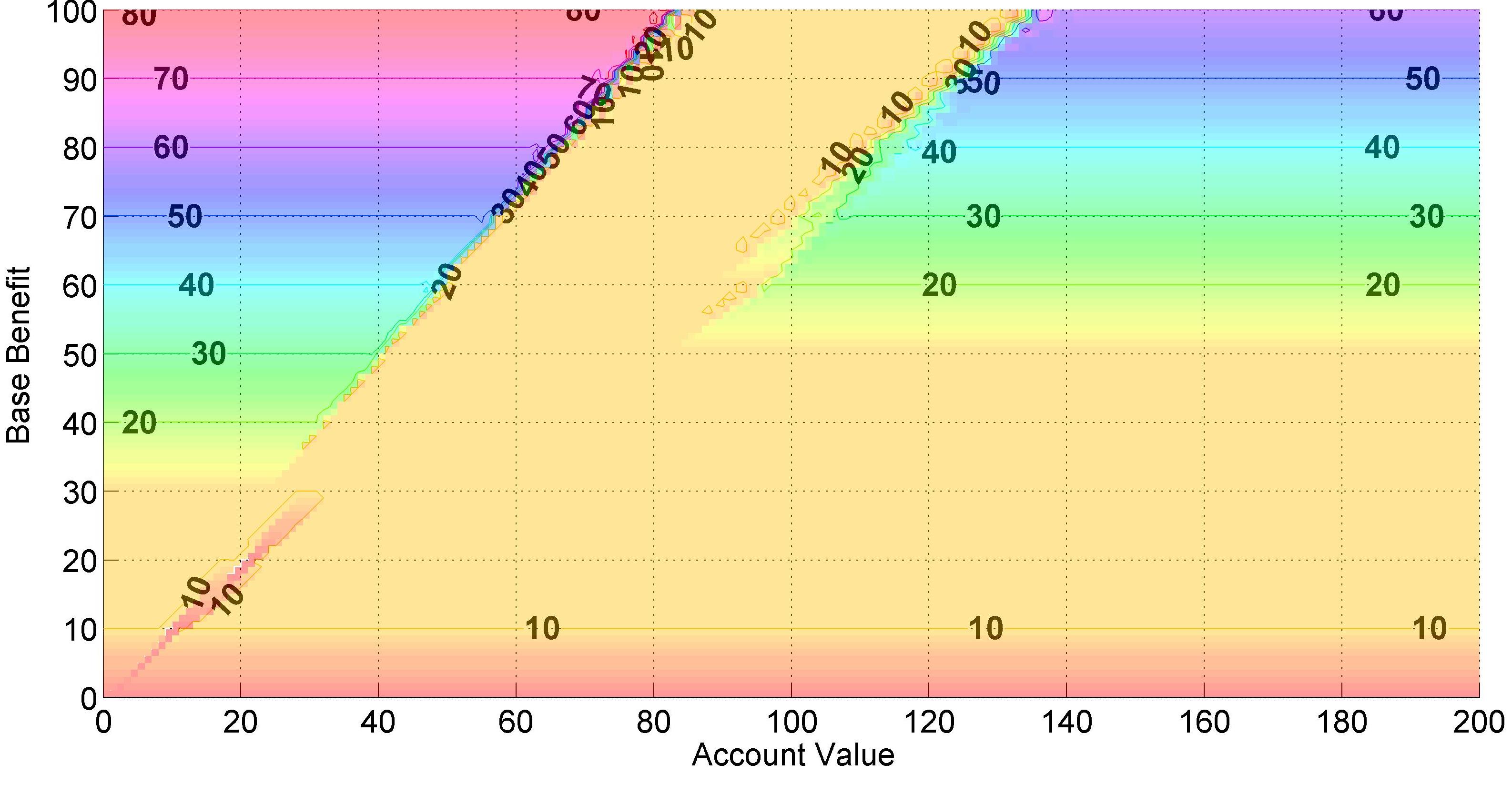
Figure 5.1: Plots of the optimal withdrawals at time $t=1$ for the BS HW model according to different values of $r_{1}$: from the top to the bottom $r_{1}=0.03$, $r_{1}=0.05$ and $r_{1}=0.07$. The parameters used to obtain these plots are the same as for Delta calculation for case $T_{2}=10$, $WDF=1$: see Tables 4, 6 and 17 .

In Figure 5.1 and 5.2 we calculated the optimal withdrawal for the GMWB-CF product with $\left(T_{2},WF\right)=\left(10,1\right)$ for both the BS HW model and Heston model. We used HPDE methods to obtain these plots: we chose three nodes of the tree around the initial value at time $t=1$ and we used the best withdrawals to get these plots.

We remark that these plots are very similar to those proposed in [9]: we note the same structure around the bisector and the wide region of regular withdrawal.

$T_{2}$ $WF=1$ $WF=2$ HMC SMC HPDE APDE BM HMC SMC HPDE APDE BM $5$ A $226.22\pm 3.04$ $223.88\pm 2.73$ $282.19$ $278.25$ $282.00$ $244.75\pm 5.85$ $242.09\pm 5.78$ $320.54$ $313.90$ $319.00$ B $255.42\pm 2.36$ $256.27\pm 2.25$ $282.24$ $276.29$ $277.53\pm 5.15$ $275.53\pm 5.12$ $320.44$ $320.59$ C $266.97\pm 1.71$ $265.12\pm 1.65$ $282.28$ $280.55$ $\pm 1.54$ $310.22\pm 3.58$ $308.76\pm 3.67$ $320.35$ $320.14$ $\pm 1.69$ D $275.83\pm 1.31$ $272.62\pm 1.23$ $282.32$ $282.63$ $312.12\pm 2.82$ $311.16\pm 2.72$ $320.33$ $320.73$ $10$ A $128.40\pm 4.58$ $130.58\pm 4.01$ $163.54$ $160.38$ $162.51$ $142.01\pm 11.5$ $141.73\pm 10.6$ $194.56$ $192.57$ $186.42$ B $144.12\pm 3.81$ $145.35\pm 3.71$ $163.03$ $157.76$ $146.20\pm 5.09$ $149.63\pm 4.95$ $190.76$ $190.90$ C $155.56\pm 2.72$ $155.54\pm 2.80$ $162.92$ $159.72$ $\pm 1.23$ $165.58\pm 3.97$ $169.64\pm 3.87$ $189.66$ $188.87$ $\pm 1.39$ D $156.97\pm 1.99$ $155.34\pm 2.02$ $162.86$ $157.37$ $182.37\pm 3.31$ $180.42\pm 3.16$ $189.47$ $188.24$ $20$ A $65.58\pm 4.45$ $65.77\pm 5.52$ $90.67$ 62.10 $84.01$ $92.16\pm 24.50$ $18.64\pm 21.96$ $109.26$ 13.72 $98.96$ B $65.50\pm 3.13$ $67.69\pm 3.57$ $86.92$ $87.53$ $80.34\pm 12.31$ $79.69\pm 19.48$ $106.77$ 31.67 C $75.87\pm 2.72$ $76.31\pm 2.67$ $86.11$ $86.42$ $\pm 1.03$ $84.79\pm 6.22$ $83.28\pm 5.10$ $106.04$ $71.80$ $\pm 1.64$ D $78.89\pm 2.14$ $81.15\pm 2.44$ $85.73$ $85.75$ $89.68\pm 4.30$ $92.43\pm 4.15$ $104.49$ $95.82$

HMC SMC HPDE APDE A $29$ s $31$ s $31$ s $30$ s B $121$ s $124$ s $121$ s $123$ s C $484$ s $484$ s $489$ s $474$ s D $1881$ s $1927$ s $1899$ s $1901$ s

Table 14: Test 4. In the first Table, the fair fee $\alpha_{g}$ in bps for the Black-Scholes Hull-White model, with annual or six-monthly withdrawal. In the second Table the run times for the case $WF=1$ , $T_{2}=10$. Finally, the plot of relative error (w.r.t. BM value) for the four methods in the same case of run-times Table. The parameters used for this test are available in Table 4 and in Table 6.

$T_{2}$ $WF=1$ $WF=2$ HMC SMC HPDE APDE BM HMC SMC HPDE APDE BM $5$ A $238.42\pm 2.36$ $238.87\pm 2.38$ $246.27$ $246.33$ $246.45$ $242.33\pm 4.37$ $245.93\pm 4.46$ $255.51$ $256.10$ $255.20$ B $237.80\pm 1.49$ $240.29\pm 1.50$ $246.58$ $246.44$ $244.68\pm 2.93$ $246.49\pm 2.96$ $256.62$ $256.43$ C $242.33\pm 1.09$ $242.95\pm 1.08$ $246.62$ $246.66$ $\pm 1.07$ $248.81\pm 2.21$ $250.94\pm 2.21$ $256.67$ $256.27$ $\pm 1.10$ D $243.42\pm 0.79$ $243.08\pm 0.77$ $246.64$ $246.68$ $253.06\pm 1.56$ $251.79\pm 1.58$ $256.70$ $256.31$ $10$ A $125.77\pm 4.03$ $123.42\pm 4.05$ $133.70$ $133.92$ $133.72$ $132.71\pm 12.0$ $119.84\pm 11.1$ $137.85$ $146.61$ $137.00$ B $126.16\pm 2.47$ $126.92\pm 2.51$ $133.89$ $133.91$ $118.80\pm 4.59$ $122.60\pm 4.57$ $138.12$ $139.39$ C $129.47\pm 1.76$ $130.41\pm 1.73$ $133.98$ $133.96$ $\pm 0.86$ $125.17\pm 3.07$ $124.11\pm 2.97$ $138.29$ $138.36$ $\pm 0.87$ D $132.89\pm 1.21$ $132.36\pm 1.22$ $134.02$ $133.99$ $130.63\pm 2.25$ $130.27\pm 2.32$ $138.41$ $138.35$ $20$ A $37.68\pm 11.94$ $37.46\pm 9.74$ $72.25$ $74.11$ $69.35$ $82.48\pm 26.34$ $61.22\pm 28.49$ $74.54$ $99.35$ $71.82$ B $64.51\pm 3.84$ $69.22\pm 2.44$ $71.05$ $72.30$ $70.71\pm 7.75$ $67.08\pm 8.48$ $73.00$ $86.01$ C $66.85\pm 3.19$ $66.13\pm 2.47$ $71.12$ $71.57$ $\pm 0.72$ $65.25\pm 3.40$ $66.50\pm 4.05$ $73.12$ $77.08$ $\pm 1.05$ D $64.18\pm 2.55$ $66.88\pm 2.18$ $71.15$ $71.69$ $61.27\pm 2.56$ $62.16\pm 2.77$ $73.24$ $74.60$

HMC SMC HPDE APDE A $32$ s $32$ s $29$ s $30$ s B $123$ s $124$ s $122$ s $118$ s C $483$ s $475$ s $474$ s $495$ s D $1903$ s $1882$ s $1923$ s $1947$ s

Table 15: Test 5. In the first Table, the fair fee $\alpha_{g}$ in bps for the Heston model, with annual or six-monthly withdrawal. In the second Table the run times for the case $WF=1$ , $T_{2}=10$. Finally, the plot of relative error (w.r.t. BM value) for the four methods in the same case of run-times Table. The parameters used for this test are available in Table 4 and in Table 8.

$T_{2}$	$WF=1$	$WF=2$
$5$	$350$	$350$
$10$	$200$	$200$
$20$	$150$	$150$

Table 16: The $\alpha_{g}$ values used for Delta calculation in the Dynamic BS HW case (bps).

$T_{2}$		$WF=1$					$WF=2$
		HMC	SMC	HPDE	APDE	BM	HMC	SMC	HPDE	APDE	BM
$5$	A	$4986\pm 311$	$4790\pm 310$	$4474$	$4465$	$4514$	$4753\pm 537$	$4117\pm 429$	$4191$	$4187$	$4181$
	B	$4455\pm 171$	$4443\pm 179$	$4477$	$4469$		$4220\pm 182$	$4362\pm 222$	$4196$	$4191$
	C	$4385\pm 130$	$4420\pm 122$	$4478$	$4473$	$\pm 62$	$4057\pm 196$	$3987\pm 170$	$4198$	$4195$	$\pm 68$
	D	$4319\pm 103$	$4432\pm\phantom{0}94$	$4478$	$4476$		$4158\pm 167$	$4235\pm 170$	$4198$	$4198$
$10$	A	$4734\pm 656$	$5152\pm 543$	$4630$	$4625$	$4593$	$4612\pm 946$	$3881\pm 817$	$4270$	$4325$	$4291$
	B	$4577\pm 320$	$4367\pm 307$	$4636$	$4616$		$4628\pm 460$	$3846\pm 362$	$4296$	$4316$
	C	$4665\pm 259$	$4548\pm 240$	$4639$	$4631$	$\pm 112$	$3898\pm 310$	$4122\pm 303$	$4304$	$4300$	$\pm 123$
	D	$4517\pm 178$	$4537\pm 175$	$4639$	$4635$		$4492\pm 329$	$4201\pm 276$	$4306$	$4304$
$20$	A	$4053\pm 302$	$4223\pm 112$	$4129$	$4149$	$4083$	$4152\pm 150$	$4037\pm 144$	$3639$	$4062$	$3857$
	B	$4370\pm 105$	$4253\pm 108$	$4153$	$4118$		$4095\pm\phantom{0}74$	$4039\pm\phantom{0}68$	$3752$	$3924$
	C	$4046\pm 332$	$4011\pm 326$	$4157$	$4150$	$\pm 143$	$4078\pm\phantom{0}72$	$4049\pm\phantom{0}60$	$3766$	$3803$	$\pm 211$
	D	$3980\pm 268$	$3857\pm 242$	$4157$	$4145$		$3434\pm 294$	$3659\pm 332$	$3780$	$3798$

Table 17: Test 6. Delta calculation for the Dynamic BS HW case. All results must be multiplied by $10^{-4}$. The parameters used for this test are available in Table 4, 17 and in Table 8.

$T_{2}$	$WF=1$	$WF=2$
$5$	$300$	$300$
$10$	$150$	$150$
$20$	$100$	$100$

Table 18: The $\alpha_{g}$ values used for Delta calculation in the Dynamic Heston case (bps).

$T_{2}$		$WF=1$					$WF=2$
		HMC	SMC	HPDE	APDE	BM	HMC	SMC	HPDE	APDE	BM
$5$	A	$5732\pm\phantom{0}40$	$5727\pm\phantom{0}26$	$5629$	$5631$	$5637$	$5878\pm\phantom{0}97$	$5803\pm\phantom{0}62$	$5571$	$5577$	$5599$
	B	$5715\pm\phantom{0}28$	$5699\pm\phantom{0}27$	$5628$	$5630$		$5678\pm\phantom{0}88$	$5603\pm\phantom{0}78$	$5570$	$5572$
	C	$5614\pm\phantom{0}49$	$5668\pm\phantom{0}66$	$5628$	$5629$	$\pm 26$	$5674\pm 122$	$5635\pm\phantom{0}78$	$5570$	$5570$	$\pm 25$
	D	$5607\pm\phantom{0}44$	$5653\pm\phantom{0}55$	$5628$	$5628$		$5695\pm 103$	$5618\pm\phantom{0}63$	$5569$	$5570$
$10$	A	$6082\pm 179$	$6103\pm 157$	$6007$	$6009$	$5983$	$6918\pm 712$	$6083\pm 392$	$5938$	$5915$	$5914$
	B	$5949\pm 133$	$5886\pm 125$	$6006$	$6007$		$6225\pm 263$	$6058\pm 142$	$5936$	$5942$
	C	$5909\pm 117$	$6062\pm 136$	$6005$	$6006$	$\pm 58$	$5779\pm 151$	$6026\pm 116$	$5936$	$5939$	$\pm 55$
	D	$6008\pm 113$	$6059\pm\phantom{0}97$	$6004$	$6005$		$5980\pm 121$	$5840\pm 114$	$5936$	$5937$
$20$	A	$5604\pm 480$	$5658\pm 383$	$5636$	$5644$	$5635$	$4162\pm 987$	$5886\pm 831$	$5540$	$5122$	$5343$
	B	$5428\pm 405$	$5855\pm 433$	$5635$	$5642$		$5056\pm 362$	$5543\pm 437$	$5540$	$5382$
	C	$5410\pm 297$	$5571\pm 206$	$5635$	$5640$	$\pm 126$	$5421\pm 306$	$5297\pm 369$	$5542$	$5543$	$\pm 174$
	D	$5734\pm 213$	$5571\pm 199$	$5635$	$5638$		$5379\pm 226$	$5416\pm 198$	$5543$	$5550$

Table 19: Test 6. Delta calculation for the Dynamic Heston case. All results must be multiplied by $10^{-4}$. The parameters used for this test are available in Table 4, 19 and in Table 8.

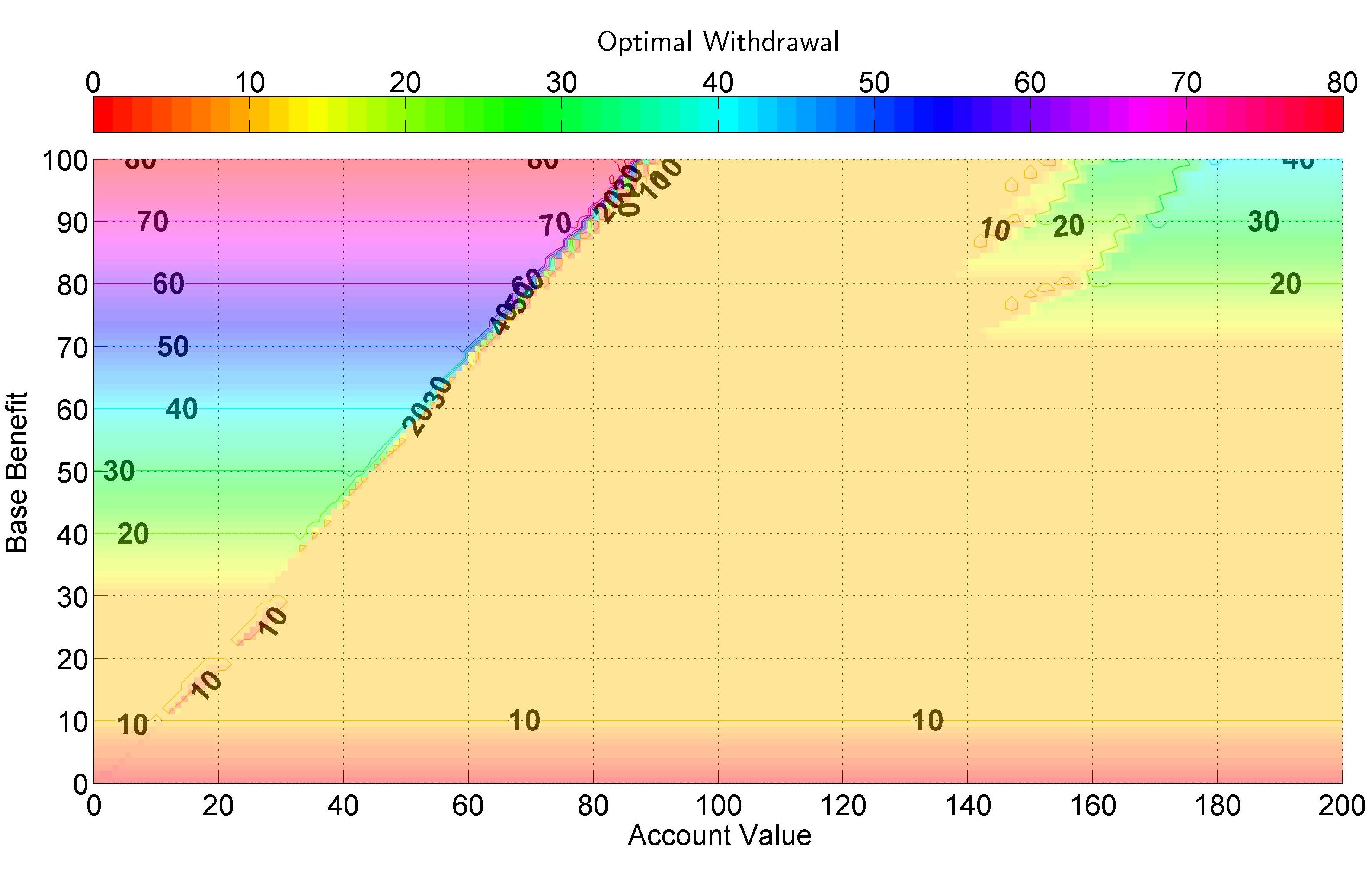
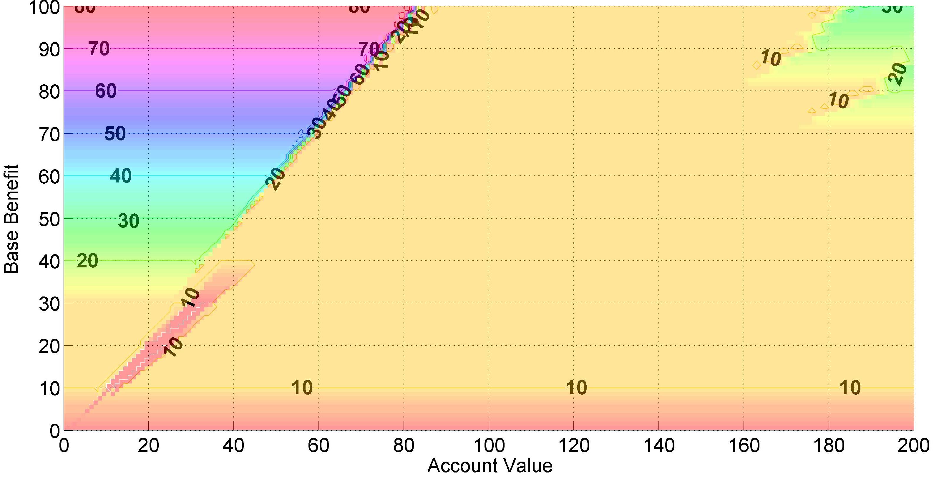
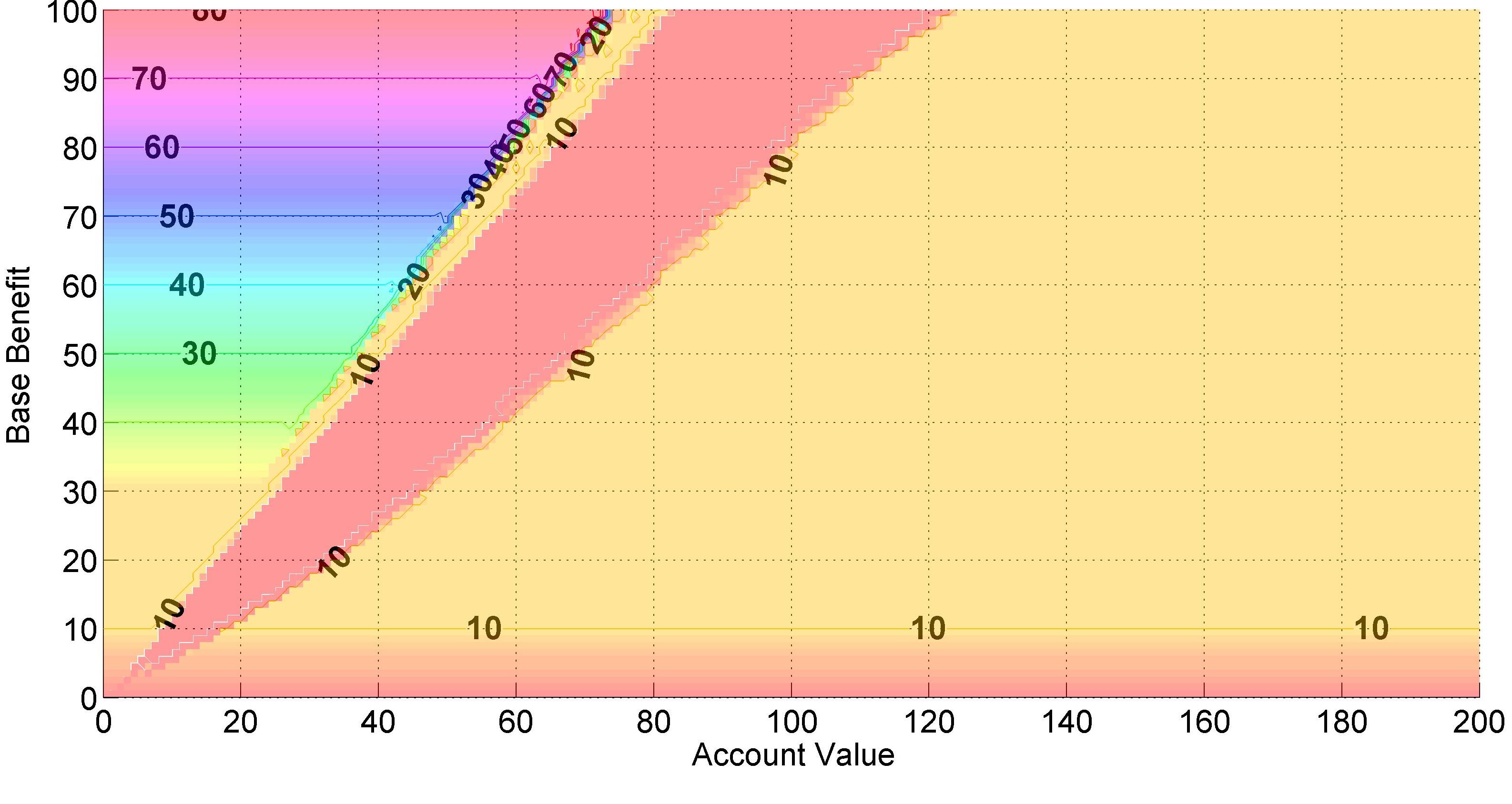
Figure 5.2: Plots of the optimal withdrawals at time $t=1$ for the Heston model according to different values of the volatility $v_{1}$: from the top to the bottom $v_{1}=0$, $v_{1}=0.04$ and $v_{1}=0.16$. The parameters used to obtain these plots are the same as for Delta calculation for case $T_{2}=10$, $WDF=1$: see Tables 4, 8 and 19.

5.3 Static Withdrawal and Optimal Surrender for GMWB-YD

In the Static Withdrawal case we suppose the PH to withdrawal exactly at the guaranteed rate, while in Optimal surrender case, the PH can stop the contract at each event time.

The Tests 7 and 8 are inspired by [17]: in their article, Yang and Dai price a GMWB contract both in Static and Dynamic (optimal surrender) framework, under the Black Scholes model. First we priced their products for different maturities and withdrawal rates, in Black and Scholes model to get a reference price in this model and to compare our results with the author’s ones. We used a standard Monte Carlo method and a standard PDE method for the Black Scholes model. Then, we add stochastic volatility and stochastic interest rate. Model parameters are available in Table 21, and the values of $\alpha_{g}$ that we got are given in Table 21.

We dealt with four numerical cases: deferred or not and Static behavior or Surrendering.

We note that using different methods (a simple Monte Carlo approach, and a PDE method for the Black-Scholes model) we didn’t obtain the same results of Yang and Dai in the case $\left(T_{1},T_{2}\right)=\left(10,25\right)$. Probably we misunderstood some contract specifications about the deferred case. We priced those products both using similarity reduction (see Section 2.5) and without, obtaining the same results. We would remark that Yang and Dai didn’t use this technique for their product.

Contract times $\left(T_{1},T_{2}\right)$	$\left(0,25\right)$ or $\left(10,25\right)$		GMW $G$	$\frac{\max\left[P,W_{T_{1}}\right]}{T_{2}-T_{1}}$
Withdrawal Frequency $WF$	1 Year		$m$	$1.0$
Initial account value $A_{0}$	$100.0$		$S_{0}$	$100.0$
Initial Premium	$100.0$		$r$	$0.0325$
Withdrawal penalty $\kappa$	$0.10$		$\sigma$	$0.30$
PH’s behavior	Static or Surrendering		Mortality	OFF

Table 20: Parameters used by Yang and Dai in [17].

$\left(T_{1},T_{2}\right)$	Static			surrendering
	PDE	MC	YD	PDE	MC	YD
$\left(0,25\right)$	$102.02$	$101.95\pm 0.21$	$102$	$158.28$	$157.33\pm 0.41$	$158$
$\left(10,25\right)$	$254.01$	$253.99\pm 0.16$	$170$	$305.35$	$305.26\pm 0.50$	$248$

Table 21: Fair bp values of $\alpha_{g}$ in Black Scholes model, for GMWB-YD with the same parameters as in [9].

5.3.1 Test 7: GMWB-YD in the Black-Scholes Hull-White Model

In the conclusion of their paper [17], Yang and Dai proposed themselves to evaluate their contract including stochastic interest rate. That’s what we do in our paper, and in Test 7 we present some numerical results about GMWB-YD pricing. Contract specifications are shown in Table 21, model parameters in Table 23 and the fair values of $\alpha_{g}$ in Table 23.

All four numerical methods behaved well in the Static case, but PDE methods outperformed the others. Thing are different in the surrendering case: the Longstaff Schwartz method showed its limits: in the BS HW model the underlying and thus the account value can diffuse so much in $25$ years and the regression over such a wide set of values is stiff. PDE methods proved to be reliable and stable, especially in case $\left(T_{1},T_{2}\right)=\left(0,25\right)$ where $25$ regressions are required.

5.3.2 Test 8: GMWB-YD in the Heston Model

After pricing the GMWB-CF product in the BS and BS HW model, then we did it in the Heston model. Contract specifications are shown in Table 21, model parameters in Table 25 and the fair values of $\alpha_{g}$ in Table 25.

Like the previous test, all four numerical methods behaved well in the Static case; HPDE and APDE outperformed the others and proved to be equivalent in that framework. In this test, numerical results of MC methods for the surrendering case are good: probably, the least square regression is easier in the Heston case. Moreover, results in the $\left(T_{1},T_{2}\right)=\left(10,25\right)$ case are very good: in this case, the Longstaff-Schwartz algorithm requires only $15$ numerical regressions and we can simulate more scenarios than in the other case.

$S_{0}$	$r$	$curve$	$k$	$\omega$	$\rho$	$\sigma$
$100$	$0.0325$	$flat$	$1.0$	$0.2$	$-0.5$	$0.30$

Table 22: The model parameters about Test 7.

Static surrendering HMC SMC HPDE APDE BM HMC SMC HPDE APDE BM $\left(T_{1},T_{2}\right)=\left(0,25\right)$ A $83.11\pm 3.55$ $81.30\pm 2.70$ $80.79$ $80.62$ $80.65$ $94.94\pm 5.28$ $89.98\pm 4.34$ $96.04$ $95.98$ $92.95$ B $83.06\pm 2.48$ $80.05\pm 1.28$ $80.71$ $80.71$ $89.12\pm 2.20$ $91.75\pm 1.84$ $95.50$ $96.04$ C $82.49\pm 1.69$ $80.62\pm 0.57$ $80.71$ $80.72$ $\pm 0.20$ $89.55\pm 1.45$ $91.79\pm 1.34$ $95.52$ $96.08$ $\pm 0.78$ D $81.48\pm 0.75$ $80.80\pm 0.28$ $80.70$ $80.72$ $89.60\pm 1.10$ $90.22\pm 1.11$ $95.53$ $96.09$ $\left(T_{1},T_{2}\right)=\left(10,25\right)$ A $213.24\pm 3.05$ $210.58\pm 2.28$ $210.40$ $210.91$ $210.76$ $242.15\pm 6.44$ $233.16\pm 5.58$ $242.38$ $242.86$ $241.41$ B $212.68\pm 2.13$ $210.47\pm 1.11$ $210.67$ $210.99$ $244.06\pm 3.38$ $239.25\pm 2.86$ $242.83$ $243.12$ C $212.45\pm 1.44$ $210.72\pm 0.49$ $210.74$ $210.89$ $\pm 0.17$ $238.66\pm 2.02$ $239.37\pm 1.67$ $242.94$ $243.07$ $\pm 0.93$ D $211.49\pm 0.66$ $210.73\pm 0.25$ $210.75$ $210.84$ $241.61\pm 1.29$ $239.75\pm 1.27$ $242.97$ $243.04$

Table 23: Test 7. The fair fee $\alpha_{g}$ in bps for the BS HW model, with Static withdrawal or Surrendering option. The parameters used for this test are available in Table 21 and in Table 23.

$S_{0}$	$v_{0}$	$\theta$	$k$	$\omega$	$\rho$	$r$
$100$	$0.30^{2}$	$0.30^{2}$	$1.0$	$0.2$	$-0.5$	$0.0325$

Table 24: The model parameters about Test 8.

Static surrendering HMC SMC HPDE APDE BM HMC SMC HPDE APDE BM $\left(T_{1},T_{2}\right)=\left(0,25\right)$ A $104.19\pm 3.43$ $104.49\pm 3.64$ $101.17$ $101.10$ $100.71$ $142.75\pm 4.67$ $140.41\pm 4.60$ $145.58$ $145.86$ $143.71$ B $101.04\pm 2.36$ $102.43\pm 2.62$ $101.07$ $101.07$ $139.92\pm 2.97$ $138.92\pm 2.82$ $145.48$ $145.80$ C $101.49\pm 1.30$ $102.19\pm 1.42$ $101.07$ $101.08$ $\pm 0.52$ $141.57\pm 1.55$ $140.22\pm 1.61$ $145.61$ $145.78$ $\pm 0.57$ D $101.45\pm 0.75$ $101.05\pm 0.80$ $101.07$ $101.08$ $142.04\pm 1.05$ $142.41\pm 1.08$ $145.62$ $145.77$ $\left(T_{1},T_{2}\right)=\left(10,25\right)$ A $246.57\pm 2.70$ $248.46\pm 2.90$ $244.67$ $244.45$ $244.52$ $280.93\pm 5.33$ $286.79\pm 5.31$ $286.20$ $286.11$ $286.39$ B $245.51\pm 1.90$ $248.04\pm 2.11$ $244.76$ $244.68$ $285.72\pm 2.73$ $286.46\pm 2.88$ $286.46$ $286.42$ C $245.31\pm 1.03$ $245.75\pm 1.14$ $244.80$ $244.78$ $\pm 0.41$ $286.67\pm 1.70$ $285.03\pm 1.72$ $286.56$ $286.52$ $\pm 0.65$ D $245.42\pm 0.60$ $245.18\pm 0.65$ $244.81$ $244.80$ $286.54\pm 1.01$ $286.41\pm 1.01$ $286.57$ $286.60$

Table 25: Test 8. The fair fee $\alpha_{g}$ in bps for the Heston model, with Static withdrawal or Surrendering option. The parameters used for this test are available in Table 21 and in Table 25.

6 Conclusions

In this article we have developed four numerical methods to price two versions of GMWB contracts under different conditions. Regarding the stochastic model, both stochastic interest rate and stochastic volatility effects have been considered. Regarding the policy holder’s behavior, both static and dynamic strategy have been considered.

Since GMWB variable annuities are such a long maturity products, the effects of stochastic interest rate and stochastic volatility cannot be overlook. In particular, the impact of stochastic interest rate seems to be more relevant.

All four methods gave compatible results both for pricing and delta calculation. The fair hedging fee (i.e. the cost of maintaining the replicating portfolio) is determined using a sequence of parameters refinements. The PDE methods proved to be not very expensive, while MC methods proved to be more expensive. The Hybrid PDE seemed to be the more performing than the others for its convergence speed and stability of results. Also ADI PDE behaved very well but the implementation was a little harder than Hybrid PDE one; moreover the choice of the good parameters for ADI PDE was a source of troubles. In the BS HW model case, Standard MC, thanks to its exact simulation, outperformed the hybrid method while, in the Heston model case, the MC methods proved to be roughly equivalent, even if the Hybrid MC was easier to be implemented.

As we said before, PDE methods proved to be much more efficient than MC methods, especially in Dynamic case where it’s much more simple to implement the optimal withdrawal choice. In the GMWB-YD case, similarity reduction reduces the dimension of the problem to 2 and therefore PDE methods perform very well. In the GMWB-CF case similarity reduction cannot be applied and therefore pricing is an harder task, especially in the case of six-monthly withdrawal and $20$ years maturity. Anyway, we have to remark that MC methods offer a confidence interval for results, they are useful in risk measures calculation (for example VAR or ES), and they are preferred by insurance companies because of their attachment to the idea of scenario.

The use of special numerical techniques (splines, improved LS convergence) allowed to ensure the convergence containing the computational time.

A future development that could be treated is to combine stochastic interest rate and stochastic volatility: the combined model could be an element of greater realism.

We conclude by pointing out that our methods are quite flexible in that they can accommodate a wide variety of policy holder withdrawal strategies such as ones derived from utility-based models.

References

- [1] A. Alfonsi (2010). High order discretization schemes for the CIR process: application to Affine Term Structure and Heston models. Mathematics of Computation, Vol. 79, No. 269, pp. 209-237.
- [2] A. D. Andricopoulos, M. Widdicks, P. W. Duck, D. P. Newton (2004). Curtailing the Range for Lattice and Grid Methods. The Journal of Derivatives Vol. 11 Issue 4, Pag 55-61.
- [3] E. Appolloni, L. Caramellino A. Zanette (2015). A robust tree method for pricing American options with the Cox-Ingersoll-Ross interest rate model. IMA Journal of Management Mathematics Vol.26, Issue No. 4, 377-401.
- [4] A. R. Bacinello, P. Millossovich, A. Olivieri, E. Pitacco (2011). Variable annuities: A unifying valuation approach. Insurance: Mathematics and Economics 49, pp. 285-297.
- [5] A. Belanger, P. Forsyth, G. Labahn (2009). Valuing the guaranteed minimum death benefit clause with partial withdrawals. Applied Mathematical Finance 16, pp. 451-496.
- [6] M. Briani, L. Caramellino, A. Zanette (2015). A hybrid approach for the implementation of the Heston model. First published online in IMA Journal of Management Mathematics, DOI 10.1093/imaman/dpv032
- [7] M. Briani, L. Caramellino, A. Zanette (2015). Numerical approximations for Heston-Hull-White type models. Preprint, arXiv:1503.03705 .
- [8] D. Brigo, F. Mercurio (2006). Interest rate models-Theory and practice. Springer, Berlin.
- [9] Z. Chen, P. A. Forsyth (2007). A Numerical Scheme for the Impulse Control Formulation for Pricing Variable Annuities with a Guaranteed Minimum Withdrawal Benefit (GMWB). Numerische Mathematik, Vol. 109, pp. 535-569.
- [10] Z. Chen, K. Vetzal, P. Forsyth (2008). The effect of modelling parameters on the value of GMWB guarantees. Insurance: Mathematics and Economics 43, pp. 165-173.
- [11] M. Dai, Y. K. Kwok, and J. Zong (2007). Guaranteed minimum withdrawal benefit in variable annuities. Mathematical Finance, forthcoming.
- [12] P. Gaillardetz, J. Lakhmiri (2011). A new premium principle for equity indexed annuities. Journal of Risk and Insurance 78, 245-265.
- [13] L. Goudenege, A. Molent, A. Zanette (2015). Pricing and Hedging GLWB in the Heston and in the Black-Scholes with Stochastic Interest Rate Models, Working paper, http://arxiv.org/abs/1509.02686.
- [14] T. Haentjens, K. J. In ’t Hout (2012): Alternating direction implicit finite difference schemes for the Heston-Hull-White partial differential equation. The Journal of Computation Finance (83-110), Vol. 16, No. 1, Fall 2012.
- [15] S. Heston (1993): A closed-form solution for options with stochastic volatility with applications to bond and currency options. The Review of Financial Studies, Vol. 6, No. 2, pp. 327-343.
- [16] J. Hull, A. White (1994). Numerical procedures for implementing term structure models I: single factor models. The Journal of Derivatives Fall, 716.
- [17] S. S. Yang, T. S. Dai (2013). A flexible tree for evaluating guaranteed minimum withdrawal benefits under deferred life annuity contracts with various provisions. Insurance: Mathematics and Economics, Vol. 52, pp. 231-242.
- [18] F. A. Longstaff, E. S. Schwartz (2001). Valuing american options by simulation: a simple least-squares approach. The Review of Financial Studies Spring 2001, Vol. 14, No. 1, pp. 113-147.
- [19] M. A. Milevsky, T. S. Salisbury (2006). Financial valuation of guaranteed minimum withdrawal benefits. Insurance: Mathematics and Economics 38, pp. 21-38.
- [20] D. B. Nelson, K. Ramaswamy (1990). Simple binomial processes as diffusion approximations in financial models. The Review of Financial Studies, Vol. 3, No. 3, pp. 393-430.
- [21] V. Ostrovski (2013). Efficient and exact simulation of the Hull-White model. Available at SSRN: http://ssrn.com/abstract=2304848 or http://dx.doi.org/10.2139/ssrn.2304848.
- [22] P. Shah, D. Bertsimas (2008). An analysis of the guaranteed withdrawal benefits for life option. Working paper, Sloan School of Management, MIT.
- [23]