Number-resolved master equation approach to quantum measurement
and quantum transport

Abstract

In addition to the well-known Landauer-Büttiker scattering theory and the nonequilibrium Green’s function technique for mesoscopic transports, an alternative (and very useful) scheme is quantum master equation approach. In this article, we review the particle-number ($n$)-resolved master equation ($n$-ME) approach and its systematic applications in quantum measurement and quantum transport problems. The $n$-ME contains rich dynamical information, allowing efficient study of topics such as shot noise and full counting statistics analysis. Moreover, we also review a newly developed master equation approach (and its $n$-resolved version) under self-consistent Born approximation. The application potential of this new approach is critically examined via its ability to recover the exact results for noninteracting systems under arbitrary voltage and in presence of strong quantum interference, and the challenging non-equilibrium Kondo effect.

I Introduction

Quantum master equation

is typically applied for the reduced state evolution of an open quantum system, e.g., in quantum optics and quantum dissipation studies Car93 ; Walls94 . This formalism is also particularly appropriate for studying quantum measurements, where the measured subsystem is the system of interest, and the apparatus is an environment. In this context, in most cases, some internal degrees of freedom of the apparatus should be retained, which may result in certain back-action effects. Moreover, for quantum measurement, extra issues should be taken into account, such as the readout characteristics of the measurement and the stochastic evolution of the measured state conditioned on the stochastic results of measurement WM09 .

An interesting solid-state application of quantum measurement is to measure charge qubits using a mesoscopic detector, which can be either a quantum-point-contact (QPC) detector Gur97 ; Win97 ; Moz02 ; Gur03 or a single electron transistor (SET) Dev00 ; Sch98 ; Sch01 ; Ston02 . For realistic applications of such measurement, the non-trivial correlation between the detector and qubit has been the focus of extensive studies Gur97 ; Gur03 ; Kor01a ; Goa01a . For instance, for the qubit-QPC setup, if the energy transfer between the detector and qubit is ignored, the qubit may relax to invalid statistical mixture Shn02 ; Sta03 ; Ave04 ; Li04 .

Moreover, for this type of measurement, we can construct a particle-number($n$)-resolved master equation ($n$-ME) scheme. That is, by properly clarifying the subspace of the apparatus states in association with the number of electrons transmitted, one can obtain Li05 ; Li05b

$$\dot{\rho}^{(n)}(t)= -i\mathcal{L}\rho^{(n)}(t)-\sum_{j=0,\pm 1}\mathcal{R}_{j}\,\rho^{(n+j)}(t).$$ (1)

Here, $\rho^{(n)}$ is the (reduced) qubit state conditioned on the number of electrons “$n$” transmitted in the detector. The Liouvillian $\mathcal{L}$ is the well-known commutator defined by the system Hamiltonian $H_{S}$. The superoperators $\mathcal{R}_{j}$ are associated with the tunneling processes in the transport detector, which have explicit forms, as given in Li05 . With the knowledge of $\rho^{(n)}(t)$, one is able to carry out the various readout characteristics of the measurement, by noting that the distribution function of the transmitted electrons is related with the $n$-conditioned density matrix as $P(n,t)=\mbox{Tr}[\rho^{(n)}(t)]$, where the trace is over the system states.

For the quantum measurement discussed above, the detector itself is a transport device. Hence, the $n$-ME approach, Eq. (1), is a natural tool for studying quantum transport through various mesoscopic (nano-scale) devices. In this context, however, the quantum coherence and/or many-body interaction effects may more significantly affect the transport properties and device functionalities. Simply, the master equation approach is appropriate for quantum transport mainly because we can regard the central device as the system of interest, and the transport leads (reservoirs) as the generalized environment.

Compared to the well-known Landauer-Büttiker theory Dat95 and the nonequilibrium Green’s function formalism Jau96 , the master equation approach (especially the $n$-ME formulation Gur96b ; Gur96a ) has been very useful for studying quantum noise in transport rev0003 ; Lev9396 ; Naz01 ; But02 ; Sam05 ; Sch0506 ; Bel05 ; Bk00 ; Bel04 ; Bla04 ; Jau04 ; Jau05 ; Bee06 ; Li07 ; Ens06 . One may note that, beyond the usual (average) current, current fluctuations in mesoscopic transport can provide useful information for the relevant mechanisms. Moreover, a fascinating approach, known as full counting statistics (FCS) analysis Lev9396 , can conveniently yield all the statistical cumulants of the number of transferred charges Naz01 ; But02 ; Sam05 ; Sch0506 ; Bel05 ; Bk00 ; Bel04 ; Bla04 ; Jau04 ; Jau05 ; Bee06 ; Li07 . The FCS has been demonstrated experimentally for transport through quantum dots Ens06 .

In essence, the $n$-ME provides an important distribution function via $P(n,t)=\mbox{Tr}[\rho^{(n)}(t)]$, which contains rich information and allows for convenient calculation of not only the transport current, but also the noise spectrum and counting statistics. For instance, for the latter, all orders of the cumulants of the transmitted electrons can be calculated by using $e^{-{\cal F}(\chi,t)}=\sum_{n}P(n,t)e^{in\chi}$, where $\chi$ is the counting field and ${\cal F}(\chi,t)$ is the cumulant generating function (CGF).

In this article, we briefly review the $n$-ME approach and its applications in quantum measurement and quantum transport problems. In Sec. II, for the qubit-QPC setup and general quantum transport system, we first review the key idea and main procedures for constructing the $n$-ME formalism, and then outline the methods of calculating the measurement/transport current and noise spectrum (using MacDonald’s formula). Particular attention will be given to decomposition of the $n$-dependent subspaces of the reservoir states and the consequences of the closed circuit nature, which would significantly affect the reservoir state averages. In Sec. III, we discuss the application of the $n$-ME to two measurement setups in detail, i.e., a qubit measured by QPC and SET detectors. In Sec. IV, we further discuss the application of the $n$-ME to quantum transport by using the double-dot Aharonov-Bohm (DDAB) interferometer and Majorana fermion (MF) probe as examples. In Sec. V, we review the newly proposed self-consistent Born approximation based master equation (SCBA-ME) approach to quantum transport; the SCBA-ME scheme goes beyond the usual master equation approach under the standard Born approximation which, for instance, can recover the exact results of quantum transport through noninteracting systems and predict the challenging non-equilibrium Kondo effect for transport through Anderson impurity (interacting dots). Finally, in Sec. VI we present our concluding remarks.

II General Formalism

In this section,

we review the construction of the $n$-ME formalism, and outline the methods of applying it to calculate the measurement/transport current and noise spectrum.

II.1 Number($n$)-Resolved Master Equation

II.1.1 Set-up (I): Qubit measurement using QPC detector

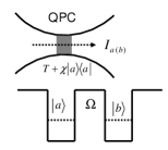
Figure 1: Schematic for a qubit (coupled quantum dots) measured by quantum point contact detector.

For the sake of generality,

we formally consider an arbitrary quantum system measured using a QPC detector. The whole setup can be described by the Hamiltonian as follows Li05 :

$$H = H_{0}+H^{\prime},$$ (2a)

$$H_{0} = H_{s}+\sum_{k}(\epsilon^{L}_{k}c^{\dagger}_{k}c_{k}+\epsilon^{R}_{k}d^{\dagger}_{k}d_{k}),$$ (2b)

$$H^{\prime} = \sum_{k,q}[T_{qk}\{|\psi_{s}\rangle\langle\psi_{s}|\}d^{\dagger}_{q}c_{k}+\mbox{H.c.}].$$ (2c)

In this decomposition, the free part of the total Hamiltonian $H_{0}$ contains the Hamiltonians of the measured system $H_{s}$ and the QPC reservoirs (the last two terms). The Hamiltonian $H^{\prime}$ describes electron tunneling through the QPC, e.g., from state $|k\rangle$ in the left reservoir to state $|q\rangle$ in the right one, with a tunneling amplitude of $T_{qk}\{|\psi_{s}\rangle\langle\psi_{s}|\}$ which may depend on the state $|\psi_{s}\rangle$ of the observable.

Regarding the tunneling Hamiltonian $H^{\prime}$ as a perturbation, on the basis of the second-order Born expansion, we can derive a formal equation for the reduced density matrix as Yan98

$$\dot{\rho}(t)=-i{\cal L}\rho(t)-\int^{t}_{0}d\tau\langle{\cal L}^{\prime}(t){\cal G}(t,\tau){\cal L}^{\prime}(\tau){\cal G}^{\dagger}(t,\tau)\rangle\rho(t).$$ (3)

Here, the Liouvillian superoperators are defined as ${\cal L}(\cdots)\equiv[H_{s},(\cdots)]$, ${\cal L^{\prime}}(\cdots)\equiv[H^{\prime},(\cdots)]$, and ${\cal G}(t,\tau)(\cdots)\equiv G(t,\tau)(\cdots)G^{\dagger}(t,\tau)$ with $G(t,\tau)$ the usual propagator (Green’s function) associated with $H_{s}$. The reduced density matrix is $\rho(t)=\mbox{Tr}_{D}[\rho_{T}(t)]$, resulting from tracing all the detector degrees of freedom from the entire density matrix. However, for quantum measurement where specific readout information is to be recorded, the average should be taken over the unique class of states of the detector that is being kept track of.

The Hilbert space of the detector can be classified as follows. First, define the subspace in the absence of electron tunneling through the detector as ${\cal D}^{(0)}$, which is spanned by the product of the many-particle states of the two isolated reservoirs, formally denoted as ${\cal D}^{(0)}\equiv\mbox{span}\{|\Psi_{L}\rangle\otimes|\Psi_{R}\rangle\}$. Then, introduce the tunneling operator $f^{\dagger}\sim f^{\dagger}_{qk}=d_{q}^{\dagger}c_{k}$, and denote the Hilbert subspace corresponding to $n$-electrons tunneled from the left to the right reservoirs as ${\cal D}^{(n)}=(f^{\dagger})^{n}{\cal D}^{(0)}$, where $n=1,2,\cdots$. The entire Hilbert space of the detector is ${\cal D}=\oplus_{n}{\cal D}^{(n)}$.

With the above classification of the detector states, the average over states in ${\cal D}$ in Eq. (3) is replaced with states in the subspace ${\cal D}^{(n)}$, leading to a conditional master equation Li05

$$\dot{\rho}^{(n)}(t) = -i{\cal L}\rho^{(n)}(t)-\int^{t}_{0}d\tau\mbox{Tr}_{D^{(n)}}[{\cal L}^{\prime}(t){\cal G}(t,\tau)$$ (4)

$$\times{\cal L}^{\prime}(\tau){\cal G}^{\dagger}(t,\tau)\rho_{T}(t)].$$

Here, $\rho^{(n)}(t)=\mbox{Tr}_{D^{(n)}}[\rho_{T}(t)]$, which is the reduced density matrix of the measured system conditioned on the number of electrons tunnelled through the detector until time $t$. Now, we transform the Liouvillian product in Eq. (4) to the conventional form:

$${\cal L}^{\prime}(t){\cal G}(t,\tau){\cal L}^{\prime}(\tau){\cal G}^{\dagger}(t,\tau)\rho_{T}(t)$$ (5)

$$= [H^{\prime}(t)G(t,\tau)H^{\prime}(\tau)G^{\dagger}(t,\tau)\rho_{T}(t)$$

$$-G(t,\tau)H^{\prime}(\tau)G^{\dagger}(t,\tau)\rho_{T}(t)H^{\prime}(t)]+\mbox{H.c.}$$

$$\equiv [I-II]+\mbox{H.c.}$$

For simplicity, we rewrite the interaction Hamiltonian as $H^{\prime}(t)=QF(t)$. Here, we have assumed the tunneling amplitude $T_{kq}$ to be real and independent of the reservoir-state “$kq$”, and denoted it by $Q$ which depends on the state of the measured system. The detector fluctuation is described by $F(t)\equiv f(t)+f^{\dagger}(t)$, with $f\equiv\sum_{kq}c^{\dagger}_{k}d_{q}$ and $f^{\dagger}\equiv\sum_{kq}d^{\dagger}_{q}c_{k}$. Two physical considerations are further made, as follows: (i) Instead of the conventional Born approximation for the entire density matrix $\rho_{T}(t)\simeq\rho(t)\otimes\rho_{D}$, we propose the ansatz $\rho_{T}(t)\simeq\sum_{n}\rho^{(n)}(t)\otimes\rho_{D}^{(n)}$, where $\rho_{D}^{(n)}$ is the density operator of the detector reservoirs with $n$-electrons tunnelled through the detector. With the ansatz of the density operator, tracing over the subspace ${\cal D}^{(n)}$ yields

$$\mbox{Tr}_{D^{(n)}}[I] = \mbox{Tr}_{D}[F(t)F(\tau)\rho_{D}^{(n)}]$$ (6a)

$$\times[QG(t,\tau)QG^{\dagger}(t,\tau)\rho^{(n)}]$$

$$\mbox{Tr}_{D^{(n)}}[II] = \mbox{Tr}_{D}[f^{\dagger}(\tau)\rho_{D}^{(n-1)}f(t)]$$ (6b)

$$\times[G(t,\tau)QG^{\dagger}(t,\tau)\rho^{(n-1)}Q]$$

$$+\mbox{Tr}_{D}[f(\tau)\rho_{D}^{(n+1)}f^{\dagger}(t)]$$

$$\times[G(t,\tau)QG^{\dagger}(t,\tau)\rho^{(n+1)}Q].$$

Here, we have utilized the orthogonality between states in different subspaces, which leads to term selection from the entire density operator $\rho_{T}$. (ii) Due to the closed nature of the detector circuit, the extra electrons tunneled into the right reservoir will flow back into the left reservoir via the external circuit. In addition, the rapid relaxation processes in the reservoirs will quickly bring the reservoirs to the local thermal equilibrium state determined by the chemical potentials. As a consequence, after the procedure (i.e., the state selection) as expressed by Eq. (6), the detector density matrices $\rho_{D}^{(n)}$ and $\rho_{D}^{(n\pm 1)}$ in Eq. (6) can be well approximated by $\rho_{D}^{(0)}$, i.e., the local thermal equilibrium reservoir state. Under this consideration, the correlation functions become, $\langle f^{\dagger}(t)f(\tau)\rangle=C^{(+)}(t-\tau)$, $\langle f(t)f^{\dagger}(\tau)\rangle=C^{(-)}(t-\tau)$, and $\langle F(t)F(\tau)\rangle=C(t-\tau)=C^{(+)}(t-\tau)+C^{(-)}(t-\tau)$. Here, $\langle\cdots\rangle$ stands for $\mbox{Tr}_{D}[(\cdots)\rho_{D}^{(0)}]$.

Under the Markovian approximation, the time integral in Eq. (4) is replaced by $\frac{1}{2}\int^{\infty}_{-\infty}$. Substituting Eqs. (5) and (6) into Eq. (4), we obtain Li05

$$\dot{\rho}^{(n)} = -i{\cal L}\rho^{(n)}-\frac{1}{2}\left\{[Q\tilde{Q}\rho^{(n)}+\mbox{H.c.}]\right.$$ (7)

$$-[\tilde{Q}^{(-)}\rho^{(n-1)}Q+\mbox{H.c.}]$$

$$\left.-[\tilde{Q}^{(+)}\rho^{(n+1)}Q+\mbox{H.c.}]\right\}.$$

Here, $\tilde{Q}^{(\pm)}=\tilde{C}^{(\pm)}({\cal L})Q$, $\tilde{C}^{(\pm)}({\cal L})=\int^{\infty}_{-\infty}dtC^{(\pm)}(t)e^{-i{\cal L}t}$, and $\tilde{Q}=\tilde{Q}^{(+)}+\tilde{Q}^{(-)}$. Under the wide-band approximation for the detector reservoirs, the spectral function $\tilde{C}^{(\pm)}({\cal L})$ can be explicitly expressed as Li04 : $\tilde{C}^{(\pm)}({\cal L})=\eta\left[x/(1-e^{-x/T})\right]_{x=-{\cal L}\mp V}$, where $\eta=2\pi g_{L}g_{R}$, and $T$ is the temperature. (Here, and in the following, we use the unit system of $\hbar=e=k_{B}=1$). In Eq. (7), the terms in $\{\cdots\}$ describe the effect of fluctuation of forward and backward electron tunneling through the detector on the measured system. In particular, the Liouvillian operator “${\cal L}$” in $\tilde{C}^{(\pm)}({\cal L})$ contains the information of energy transfer between the detector and the measured system, which correlates the energy (spontaneous) relaxation of the measured system with the inelastic electron tunneling in the detector. At high-voltage limit, formally $V\gg{\cal L}$, the spectral function $\tilde{C}^{(\pm)}({\cal L})\simeq\tilde{C}^{(\pm)}(0)$, and Eq. (7) reduce to the result derived by Gurvitz et al Gur97 ; Moz02 ; Gur03 ; Goa01a .

II.1.2 Set-up (II): Quantum transport

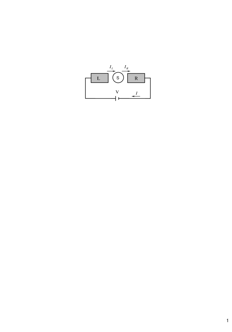
Figure 2: Schematic setup for quantum transport through a mesoscopic system.

In general,

quantum transport, schematically shown in Fig. 2, can be described by the following Hamiltonian:

$$H = H_{S}(a_{\mu}^{\dagger},a_{\mu})+\sum_{\alpha=L,R}\sum_{\mu k}\epsilon_{\alpha\mu k}d^{\dagger}_{\alpha\mu k}d_{\alpha\mu k}$$ (8)

$$+\sum_{\alpha=L,R}\sum_{\mu k}(t_{\alpha\mu k}a^{\dagger}_{\mu}d_{\alpha\mu k}+\rm{H.c.}).$$

Here, $H_{S}$ is the central system (device) Hamiltonian, which can be quite general (e.g., includes many-body interactions). $a^{\dagger}_{\mu}$ ($a_{\mu}$) is the creation (annihilation) operator of electrons in state $|\mu\rangle$, which indicates both the orbital and spin degrees of freedom. The second and third terms describe, respectively, the two (left and right) leads (reservoirs) and the tunneling between them and the central system. The lead electrons are also attached here by index “$\mu$” to characterize their possible correlation with the system states. For instance, this will be the typical situation for spin-dependent transport.

If we introduce $F_{\mu}=\sum_{\alpha k}t_{\alpha\mu k}d_{\alpha\mu k}\equiv f_{L\mu}+f_{R\mu}$ and express the tunneling Hamiltonian as

$$H^{\prime} = \sum_{\mu}\left(a^{\dagger}_{\mu}F_{\mu}+\rm{H.c.}\right),$$ (9)

then, by considering this tunneling Hamiltonian as a perturbation, the second-order Born expansion results in an unconditional master equation for the reduced density matrix of the same form of Eq. (3).

To construct a conditional (i.e. particle-number-resolved) master equation, one should keep track of the number of electrons that arrive at the collector. Let us classify the Hilbert space of the electrodes as follows. First, we define the subspace in the absence of electrons at the collector as “$B^{(0)}$”, which is spanned by the product of all many-particle states of the two isolated reservoirs, formally denoted as $B^{(0)}\equiv\mbox{span}\{|\Psi_{L}\rangle\otimes|\Psi_{R}\rangle\}$. Then, we introduce the Hilbert subspace “$B^{(n)}$” ( $n=1,2,\cdots$), corresponding to $n$-electrons at the collector. The entire Hilbert space of the two electrodes is $B=\oplus_{n}B^{(n)}$.

With this type of classification for the reservoir states, the average over states in the entire Hilbert space “$B$” is replaced with states in the subspace “$B^{(n)}$”, leading to a conditional master equation Li05b

$$\dot{\rho}^{(n)}(t) = -i{\cal L}\rho^{(n)}(t)-\int^{t}_{0}d\tau\mbox{Tr}_{B^{(n)}}[{\cal L}^{\prime}(t){\cal G}(t,\tau)$$ (10)

$$\times{\cal L}^{\prime}(\tau){\cal G}^{\dagger}(t,\tau)\rho_{T}(t)].$$

Here, $\rho^{(n)}(t)=\mbox{Tr}_{B^{(n)}}[\rho_{T}(t)]$, where $\rho_{T}(t)$ is the state of the whole system. $\rho^{(n)}(t)$ is the reduced density matrix of the central system conditioned on the number of electrons arriving at the collector until time $t$.

As for the qubit-QPC problem, two important considerations are made, as follows: (i) Instead of the conventional Born approximation for the entire density matrix $\rho_{T}(t)\simeq\rho(t)\otimes\rho_{B}$, we propose the ansatz $\rho_{T}(t)\simeq\sum_{n}\rho^{(n)}(t)\otimes\rho_{B}^{(n)}$, where $\rho_{B}^{(n)}$ is the density operator of the electron reservoirs associated with $n$-electrons arrived at the collector. (ii) Due to the closed nature of the transport circuit, the extra electrons arriving at the collector will flow back into the emitter (left reservoir) via the external circuit. In addition, the rapid relaxation processes in the reservoirs will quickly bring the reservoirs to the local thermal equilibrium state determined by the chemical potentials.

Then, under the Markovian approximation, from Eq. (10), we obtain Li05b

$$\dot{\rho}^{(n)} = -i{\cal L}\rho^{(n)}-\frac{1}{2}\sum_{\mu}\left\{[a_{\mu}^{\dagger}A_{\mu}^{(-)}\rho^{(n)}+\rho^{(n)}A_{\mu}^{(+)}a_{\mu}^{\dagger}\right.$$ (11)

$$-A_{L\mu}^{(-)}\rho^{(n)}a_{\mu}^{\dagger}-a_{\mu}^{\dagger}\rho^{(n)}A_{L\mu}^{(+)}$$

$$\left.-A_{R\mu}^{(-)}\rho^{(n-1)}a_{\mu}^{\dagger}-a_{\mu}^{\dagger}\rho^{(n+1)}A_{R\mu}^{(+)}]+{\rm H.c.}\right\}.$$

Here, $A_{\alpha\mu}^{(\pm)}=\sum_{\nu}C_{\alpha\mu\nu}^{(\pm)}(\pm{\cal L})a_{\nu}$ and $A_{\mu}^{(\pm)}=\sum_{\alpha=L,R}A_{\alpha\mu}^{(\pm)}$. The spectral functions $C_{\alpha\mu\nu}^{(\pm)}(\pm{\cal L})$ are defined in terms of the Fourier transform of the reservoir correlation functions, i.e., $C_{\alpha\mu\nu}^{(\pm)}(\pm{\cal L})=\int^{\infty}_{-\infty}dtC_{\alpha\mu\nu}^{(\pm)}(t)e^{\pm i{\cal L}t}$, where $\langle f^{\dagger}_{\alpha\nu}(\tau)f_{\alpha\mu}(t)\rangle=C_{\alpha\mu\nu}^{(+)}(t-\tau)$ and $\langle f_{\alpha\mu}(t)f^{\dagger}_{\alpha\nu}(\tau)\rangle=C_{\alpha\mu\nu}^{(-)}(t-\tau)$.

The “$n$”-dependence of Eq. (11) is somehow similar to the usual rate equation, despite its operator feature. Each term in Eq. (11) can be interpreted similarly using the conventional c-number rate equation. Unlike in the Bloch equation derived by Gurvitz et al Gur96b , in Eq. (11), $\rho^{(n)}$ is also coupled to $\rho^{(n+1)}$, which is not present in Ref. Gur96b, . This difference originates from the fact that Eq. (11) is valid for non-zero temperatures.

II.2 Current and Noise Spectrum

II.2.1 Qubit measurement by QPC

With the knowledge of

$\rho^{(n)}(t)$, one can carry out the various readout characteristics of the measurement. In particular, for a qubit with $\Omega\neq 0$ and $\Omega^{-1}$ comparable to or smaller than the measurement time Sch98 , the qubit oscillation cannot be read out using the conventional single shot measurement. In this regime, continuous weak measurement is an alternative scheme to record the qubit oscillations, e.g., in the power spectrum of the output current.

First, for the ensemble-average current, simple expression is related to the unconditional density matrix $\rho(t)=\sum_{n}\rho^{(n)}(t)$. The derivation is from the fact that the current is associated with the probability distribution $P(n,t)\equiv\rm{Tr}[\rho^{(n)}(t)]$, via $I(t)=ed\bar{N}(t)/dt$, where $\bar{N}(t)=\sum_{n}nP(n,t)$. By considering the Summation over “$n$” and making use of the cyclic property under trace, we obtain Li05

$$I(t)=\sum_{n}n\mbox{Tr}[\dot{\rho}^{(n)}(t)]=\frac{1}{2}\mbox{Tr}[\bar{Q}\rho(t)Q+\mbox{H.c.}],$$ (12)

where $\bar{Q}=\tilde{Q}^{(-)}-\tilde{Q}^{(+)}$.

Second, the power spectrum of the output current can be conveniently calculated using the MacDonald’s formula Gur03 ; Li05

$$S(\omega)=2\omega\int^{\infty}_{0}dt\sin\omega t\frac{d}{dt}\left[\langle n^{2}(t)\rangle-(\bar{I}t)^{2}\right],$$ (13)

where $\bar{I}$ is the average current over time and $\langle n^{2}(t)\rangle=\sum_{n}n^{2}P(n,t)$. It can be proved that Li05

$$\frac{d}{dt}\langle n^{2}(t)\rangle=\mbox{Tr}\left[\bar{Q}\hat{N}(t)Q+\frac{1}{2}\tilde{Q}\rho(t)Q+\mbox{H.c.}\right],$$ (14)

where $\hat{N}(t)\equiv\sum_{n}n\rho^{(n)}(t)$, which can be calculated via its equation of motion Li05

$$\frac{d\hat{N}}{dt}=-i{\cal L}\hat{N}-\frac{1}{2}\left[Q,\tilde{Q}\hat{N}-\hat{N}\tilde{Q}^{\dagger}\right]+\frac{1}{2}(\bar{Q}\rho Q+\mbox{H.c.})\,.$$

Combining the above three equations, the noise spectrum $S(\omega)$ can be easily obtained via Laplace transform in terms of simple algebraic manipulations.

II.2.2 Quantum transport

For quantum transport

, based on the $n$-ME (11), a method similar to that outlined above leads to Li05b

$$I(t)=e\sum_{n}n\rm{Tr}\left[\dot{\rho}^{(n)}(t)\right]$$

$$=\frac{e}{2}\sum_{\mu}\rm{Tr}\left[\left(a^{\dagger}_{\mu}A^{(-)}_{R\mu}-A^{(+)}_{R\mu}a^{\dagger}_{\mu}\right)\rho(t)+\rm{H.c.}\right].$$ (16)

Here, the unconditional density matrix $\rho=\sum_{n}\rho^{(n)}$ satisfies the usual master equation (which can be obtained by summing up Eq. (11) over “$n$”)

$$\dot{\rho}=-i{\cal L}\rho-\frac{1}{2}\sum_{\mu}\left\{[a_{\mu}^{\dagger},A_{\mu}^{(-)}\rho-\rho A_{\mu}^{(+)}]+\rm{H.c.}\right\}.$$ (17)

Eqs. (II.2.2) and (17) can serve as a convenient starting point to compute the transport current. In practice, one can first diagonalize the central system Hamiltonian, then perform the Liouvillian operations in the eigen-state representation.

For transport, the current noise spectrum can provide additional dynamic information beyond the current itself. We know that, for time-dependent transport, the currents across the left and right junctions (between the central system and the two leads) are not necessarily equal to each other. This requires a definition for the power spectrum using the “average” current $I(t)=\alpha I_{L}(t)+\beta I_{R}(t)$, where $\alpha$ and $\beta$ are two coefficients determined by the junction capacitances Li053 , which satisfy $\alpha+\beta=1$. This leads to the noise spectrum of the current consisting of three parts Li053 : $S(\omega)=\alpha S_{L}(\omega)+\beta S_{R}(\omega)-\alpha\beta\omega^{2}S_{N}(\omega)$, where $S_{L/R}(\omega)$ is the noise spectrum of the left (right) junction current $I_{L/R}(t)$ and $S_{N}(\omega)$ is the fluctuation spectrum of the electron number $N(t)$ on the central device.

For $S_{\lambda}(\omega)$ ($\lambda=L,R$), we use the MacDonald’s formula

$$S_{\lambda}(\omega)=2\,\omega\!\int_{0}^{\infty}\!\!dt\sin(\omega t)\frac{d}{dt}[\langle n_{\lambda}^{2}(t)\rangle-(\bar{I}t)^{2}]\,,$$ (18)

where $\bar{I}$ is the stationary current and $\langle n_{\lambda}^{2}(t)\rangle=\sum_{n_{\lambda}}n_{\lambda}^{2}[\mbox{Tr}\rho^{(n_{\lambda})}(t)]=\sum_{n_{\lambda}}n_{\lambda}^{2}P(n_{\lambda},t)$. Using Eq. (11), we obtain Li053

$$\frac{d}{dt}\langle n_{\lambda}^{2}(t)\rangle=\mbox{Tr}\big{[}2\mathcal{T}^{(-)}_{\lambda}N^{\lambda}(t)+\mathcal{T}^{(+)}_{\lambda}\rho^{\rm st}\big{]},$$ (19)

where $N^{\lambda}(t)\equiv\sum_{n_{\lambda}}n_{\lambda}\rho^{(n_{\lambda})}(t)$ denotes the “number” matrix and $\rho^{\rm st}$ is the stationary state. Here, we also introduce

$$\mathcal{T}^{(\pm)}_{\lambda}(\cdots)=\frac{1}{2}\sum_{\mu}\big{[}A_{\lambda\mu}^{(-)}(\cdots)a_{\mu}^{\dagger}\pm a_{\mu}^{\dagger}(\cdots)A_{\lambda\mu}^{(+)}\big{]}\!+\!\mbox{H.c.}.$$ (20)

The final expression for $S_{\rm L/R}(\omega)$ is Li053

$$S_{\lambda}(\omega)\! = \!4\,\omega\,{\rm Im}\big{\{}{\rm Tr}\big{[}{\cal T}^{(-)}_{\lambda}\widetilde{N}^{\lambda}(\omega)\big{]}\}$$ (21)

$$+\,2\,{\rm Tr}\big{[}{\cal T}^{(+)}_{\lambda}\rho^{\rm st}\big{]}-8\,\pi\,\bar{I}^{2}\,\delta(\omega),$$

where $\widetilde{N}^{\lambda}(\omega)=\int_{0}^{\infty}dtN^{\lambda}(t)e^{i\omega t}$. The last term originates from the second term in the MacDonald’s formula in Eq. (18). $\widetilde{N}^{\lambda}(\omega)$ can be easily obtained by solving the following equation of motion in the frequency domain Li053 :

$$\frac{d}{dt}N^{\lambda}(t)=-i{\cal L}N^{\lambda}(t)-{\cal R}N^{\lambda}(t)+{\cal T}^{(-)}_{\lambda}\rho^{\rm st},$$ (22)

which gives

$$\!\!\!\!-i\omega\widetilde{N}^{\lambda}(\omega)\!\!\! = \!\!-i{\cal L}\widetilde{N}^{\lambda}(\omega)\!-\!{\cal R}\widetilde{N}^{\lambda}(\omega)\!+\!{\cal T}^{(-)}_{\lambda}\widetilde{\rho}(\omega),$$ (23)

where $\widetilde{\rho}(\omega)=i\rho^{\rm st}/\omega$.

For the charge fluctuations on the central system, the symmetrized noise spectrum can be expressed using Li053

$$S_{N}(\omega)=\omega^{2}\!\int_{-\infty}^{\infty}\!d\tau\langle\hat{N}(\tau)\hat{N}+\hat{N}\hat{N}(\tau)\rangle e^{i\omega\tau},$$ (24)

where $\langle\hat{N}(\tau)\hat{N}\rangle=\mbox{Tr}\mbox{Tr}_{\rm B}[U^{{\dagger}}(\tau)\hat{N}U(\tau)\hat{N}\rho^{\rm st}\rho_{\rm B}]$, where $U(\tau)=e^{-iH\tau}$ and $\hat{N}$ is the electron-number operator of the central system. Using the cyclic property under trace, we have $\langle\hat{N}(\tau)\hat{N}\rangle=\mbox{Tr}[\hat{N}\sigma(\tau)]$, where $\sigma(\tau)=\mbox{Tr}_{\rm B}[U(\tau)\hat{N}\rho^{\rm st}\rho_{\rm B}U^{{\dagger}}(\tau)]$. Desirably, $\sigma(\tau)$ satisfies the equation of the usual reduced density matrix. Its Fourier transform $\widetilde{\sigma}(\omega)$ can be easily solved using Li053

$$i(\omega-{\cal L})\widetilde{\sigma}(\omega)={\cal R}\widetilde{\sigma}(\omega)-\hat{N}\rho^{\rm st}.$$ (25)

Then, we have Li053

$$S_{N}(\omega)=2\omega^{2}\mbox{Re}\{{\rm Tr}\{\hat{N}[\widetilde{\sigma}(\omega)+\widetilde{\sigma}(-\omega)]\}.$$ (26)

II.3 Counting Statistics and Large-Deviation Analysis

In order to get

information in addition to the average current and current fluctuation spectrum, with the knowledge of $\rho^{(n)}(t)$ (and thus $P(n,t)$), one can perform FCS Lev9396 and large-deviation (LD) analysis LD9809 ; SM8792 ; Gar10 . For FCS analysis, the current CGF can be constructed using FCS07

$$e^{-\tilde{\cal F}(\chi,t)}=\sum_{n}P(n,t)e^{in\chi},$$ (27)

where $\chi$ is the so-called counting field. Based on the CGF, $\tilde{\cal F}(\chi,t)$, the $k_{\rm th}$ cumulant can be readily carried out via $C_{k}=-(-i\partial_{\chi})^{k}\tilde{\cal F}(\chi,t)|_{\chi=0}$. As a result, one can easily confirm that the first two cumulants, $C_{1}=\bar{n}$ and $C_{2}=\overline{n^{2}}-\bar{n}^{2}$, give rise to the mean value and the variance of the transmitted electrons, while the third one (skewness), $C_{3}=\overline{(n-\bar{n})^{3}}$, characterizes the asymmetry of the distribution. Here, $\overline{(\cdots)}=\sum_{n}(\cdots)P(n,t)$. Moreover, one can relate the cumulants to measurable quantities, e.g., the average current by $I=eC_{1}/t$, and the zero-frequency shot noise by $S=2e^{2}C_{2}/t$. In addition, the important Fano factor is simply given by $F=C_{2}/C_{1}$, which characterizes the extent of current fluctuations: $F>1$ indicates a super-Poisson fluctuating behavior, while $F<1$ indicates a sub-Poisson process.

For the LD analysis, instead of using the discrete Fourier transform in Eq. (27), one may consider $e^{i\chi n}\Rightarrow e^{-xn}$. That is, introduce the dual-function of $P(n,t)$ LD11 :

$$P(x,t)=\sum_{n}e^{-xn}P(n,t)=e^{-{\cal F}(x,t)}.$$ (28)

The real nature of the transform factor $e^{-xn}$, in contrast to the complex one, $e^{i\chi n}$, makes the resultant $P(x,t)$ somewhat resemble the partition function in statistical mechanics. Using analogous terms in statistical mechanics, in Eq. (28), the trajectories are categorized by a dynamical order parameter “$n$” or its conjugate field “$x$”. This is realized by an exponential weight similar to the Boltzmann factor, with the dynamical order parameter representing the energy or magnetization and the conjugate field representing the temperature or magnetic field.

$P(x,t)$ is called LD function in LD analysis. In statistical mechanics, the partition function measures the number of microscopic configurations accessible to the system under given conditions. For the mesoscopic transport under consideration, if we are interested in the dynamical aspects of the transport electrons, the above insight can be used for LD analysis in the time domain. That is, the LD function is a measure of the number of trajectories accessible to the “counter”, which favorably characterizes the trajectory space from multiple angles according to the effect of the conjugate field. In particular, it allows one to inspect the rare fluctuations or extreme events by tuning the conjugate field “$x$”.

We emphasize that, if one performs the conventional FCS analysis only, using either a complex transform factor $e^{i\chi n}$ or a real one $e^{-xn}$ would make no difference since the limit $\chi(x)\rightarrow 0$ will be considered at the end. However, for the LD study, we must use the real factor $e^{-xn}$, which plays a role in categorizing (selecting) the trajectories. This type of selection would enables us to perform statistical analysis for the fluctuations of sub-ensembles of trajectories. For instance, $x>0$ implies mainly selecting the inactive trajectories (with small $n$), while $x<0$ prefers the active trajectories (with large $n$). In particular, by varying $x$, the $x$-dependent statistics can reveal interesting dynamical behaviors in the time-domain. In other words, based on the distribution function $P(n,t)$, which contains complete information of all the trajectories, the LD approach, beyond the conventional FCS analysis, captures more information from $P(n,t)$ via the $x$-dependent cumulants.

From the technical point of view, similar to transforming $P(n,t)$ to $P(x,t)$, we introduce $\rho(x,t)=\sum_{n}e^{-xn}\rho^{(n)}(t)$. Then, from Eq. (1), we formally have LD11

$$\dot{\rho}(x,t)=\left[-i{\cal L}-{\cal R}_{0}-e^{x}{\cal R}_{1}-e^{-x}{\cal R}_{-1}\right]\rho(x,t).$$ (29)

This equation allows us to carry out the LD function $P(x,t)$ via $P(x,t)={\rm Tr}[\rho(x,t)]$, where the trace is over the central system states. Accordingly, we obtain the generating function ${\cal F}(x,t)=-\ln P(x,t)$ for arbitrary counting time $t$. Further, we can prove LD11

$${\cal F}_{1}(x,t) \equiv\partial_{x}{\cal F}(x,t)=\frac{1}{P(x,t)}\sum_{n}ne^{-xn}P(n,t)\equiv\langle n\rangle_{x},$$ (30a)

$${\cal F}_{2}(x,t) \equiv\partial^{2}_{x}{\cal F}(x,t)=-\langle(n-\bar{n}_{x})^{2}\rangle_{x},$$ (30b)

and more generally,

$${\cal F}_{k}(x,t)\equiv\partial^{k}_{x}{\cal F}(x,t)=(-)^{(k+1)}\langle(n-\bar{n}_{x})^{k}\rangle_{x}.$$ (30c)

Here, for brevity, we used the notation $\bar{n}_{x}$ for $\langle n\rangle_{x}$. Using these cumulants, we can define a finite-counting-time average current $I(x,t)=e{\cal F}_{1}(x,t)/t$ and the shot noise $S(x,t)=2e^{2}{\cal F}_{2}(x,t)/t$. In addition, the generalized Fano factor, $F(x,t)={\cal F}_{2}(x,t)/{\cal F}_{1}(x,t)$, will be of interest to characterize the fluctuation properties.

We notice that, in order to obtain ${\cal F}_{k}(x,t)$, we only need to determine the various $k$-th order derivatives of $P(x,t)$, $P_{k}(x,t)=\partial^{k}_{x}P(x,t)$. This is an efficient method to compute the $x$-dependent cumulants for finite counting time. That is, by performing the derivatives $\partial^{k}_{x}$ on Eq. (29) and defining $\rho_{k}(x,t)=\partial^{k}_{x}\rho(x,t)$, we obtain a set of coupled equations for $\rho_{k}(x,t)$, whose solution then gives $P_{k}(x,t)={\rm Tr}[\rho_{k}(x,t)]$.

In long counting time limit, it can be proved that ${\cal F}(x,t)\simeq t\lambda(x)$. Desirably, the asymptotic form, $P(x,t)\simeq e^{-t\lambda(x)}$, allows one to identify the LD function $\lambda(x)$ for the smallest eigenvalue of the counting matrix, i.e., the r.h.s of Eq. (29).

III Application to Quantum Measurement

In this section,

we illustrate the application of the $n$-ME to two examples of quantum measurement, i.e., for a charge qubit measured respectively by QPC and SET detectors.

III.1 Qubit Measured by QPC

Let us specify

the charge qubit as a pair of coupled quantum dots, described by the Hamiltonian $H_{\rm qu}=\epsilon_{a}|a\rangle\langle a|+\epsilon_{b}|b\rangle\langle b|+\Omega(|b\rangle\langle a|+|a\rangle\langle b|)$. We then introduce $\epsilon=(\epsilon_{a}-\epsilon_{b})/2$ and set $(\epsilon_{a}+\epsilon_{b})/2$ as the reference energy. The qubit eigen-energies are obtained as $E_{1}=\sqrt{\epsilon^{2}+\Omega^{2}}\equiv\Delta/2$ and $E_{0}=-\sqrt{\epsilon^{2}+\Omega^{2}}=-\Delta/2$. Correspondingly, the eigenstates are $|1\rangle=\cos\frac{\theta}{2}|a\rangle+\sin\frac{\theta}{2}|b\rangle$ for the excited state and $|0\rangle=\sin\frac{\theta}{2}|a\rangle-\cos\frac{\theta}{2}|b\rangle$ for the ground state, where $\theta$ is introduced using $\cos\theta=2\epsilon/\Delta$ and $\sin\theta=2\Omega/\Delta$. The coupling between the qubit and detector is characterized by $H^{\prime}=QF$, where $Q={\cal T}+\chi|a\rangle\langle a|$ and $F=\sum_{k,q}(c^{\dagger}_{k}d_{q}+\mbox{H.c.})$.

By applying Eq. (12), we obtain the stationary current for a symmetric qubit ($\epsilon=0$) as Li05

$$I_{s}=g_{0}V+g_{1}V\left[1-2\frac{G^{(-)}}{V}+\frac{\Delta}{V}\frac{G^{(-)}}{G^{(+)}}\right].$$ (31)

Here, $g_{0}=\eta({\cal T}+\chi/2)^{2}$, $g_{1}=\eta(\chi/2)^{2}$, and $G^{(\pm)}=\frac{1}{2}\left[F^{(+)}(\Delta,V)\pm F^{(-)}(\Delta,V)\right]$, with $F^{(\pm)}(\Delta,V)\equiv(\Delta\pm V)\coth(\frac{\Delta\pm V}{2T})$. At zero temperature, Eq. (31) can be further simplified. Compared with previous results Shn02 ; Sta03 , we find that under low voltage ($V<\Delta$), Eq. (31) is reduced to the same result given by Shnirman et al. Shn02 , but under $V>\Delta$ it differs from the results in Refs. Shn02, and Sta03, .

The output power spectrum $S(\omega)$ can be calculated using the MacDonald’s formula via Eqs. (13)-(II.2.1). For a symmetric qubit and denoting $S(\omega)=S_{0}+S_{1}(\omega)+S_{2}(\omega)$, we obtain Li05

$$S_{0} = 2I_{0}\coth\frac{V}{2T}+\frac{\chi^{2}\eta}{2}$$ (32a)

$$\times\left[G^{(+)}-\frac{\Delta^{2}}{G^{(+)}}-V\coth\frac{V}{2T}\right],$$

$$S_{1}(\omega) = \left[1-\frac{\Delta}{2V}\frac{G^{(-)}}{G^{(+)}}\right]\frac{I^{2}_{d}\Gamma_{d}\Delta^{2}}{(\omega^{2}-\Delta^{2})^{2}+\Gamma_{d}^{2}\omega^{2}},$$ (32b)

$$S_{2}(\omega) = \chi^{2}\eta\left[\Gamma_{d}D_{z}+\gamma\bar{I}\right]\frac{G^{(-)}}{\omega^{2}+\Gamma_{d}^{2}}.$$ (32c)

Here, three currents are defined as $I_{0}=(I_{a}+I_{b})/2$, $I_{d}=I_{a}-I_{b}$, and $\bar{I}=I_{0}-\frac{1}{4}\eta\chi^{2}\Delta G^{(-)}/G^{(+)}$, with $I_{a}=\eta({\cal T}+\chi)^{2}V$ and $I_{b}=\eta{\cal T}^{2}V$ being the detector currents corresponding to qubit states $|a\rangle$ and $|b\rangle$, respectively. The other quantities in Eq. (32) are $\Gamma_{d}=\frac{\eta\chi^{2}}{2}G^{(+)}$, $\gamma=\frac{\eta\chi^{2}}{2}\Delta$ and $D_{z}=-\Delta\sqrt{I_{a}I_{b}}/G^{(+)}-\eta\chi^{2}G^{(-)}/4$. The three noise spectrum components are, respectively, (i) the zero-frequency noise $S_{0}$, (ii) the Lorentzian spectral function $S_{1}(\omega)$ with a peak around the qubit Rabi frequency $\omega=\Delta$, and (iii) $S_{2}(\omega)$, originating from the qubit-relaxation-induced inelastic tunnelling effect in the detector. In addition to $S_{2}(\omega)$, the qubit relaxation effect is also manifested in $S_{0}$ and $S_{1}(\omega)$, i.e., giving rise to the second term of $S_{0}$ and reducing the pre-factor in $S_{1}(\omega)$ from unity. If the qubit-relaxation-induced inelastic effect is neglected or at the limit of the high bias voltage $V\gg\Delta$, Eq. (32) returns to the result obtained in previous work Kor01a ; Goa01a .

Figure 3: (a) Noise spectrum in the presence (solid curves) and absence (dashed curves) of qubit relaxation. (b) Voltage effect on the noise spectrum, particularly on the peak-to-pedestal ratio (inset, where the solid and dashed curves correspond to the presence and absence of qubit relaxation). The results in (a) and (b) are obtained, respectively, by altering $\chi$ (for a fixed voltage $V=2\Delta$ ) and the voltage $V$ (for a fixed $\chi=0.1\Delta$). Other parameters: $g_{L}=g_{R}=2.5/\Delta$, and $T=\Delta$.

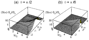
Figure 4: 3D-plot of the noise spectra for (a) the symmetric and (b) the asymmetric qubit. Parameters: $g_{L}=g_{R}=2.5/\Delta$, $\chi=0.1\Delta$, and $T=\Delta$.

The measurement-induced relaxation effects of the qubit are shown in Fig. 3. The major effect of the qubit relaxation shown in Fig. 3(a) is the lowering of the entire noise spectrum in qualitative consistence with the findings of Gurvitz et al Gur03 , where an external thermal bath is introduced to cause qubit relaxation. However, the spontaneous relaxation discussed here does not diminish the telegraph noise peak near zero frequency in the incoherent case, which implies the presence of the Zeno effect, in contrast to the major conclusion of Ref. Gur03, . In addition, the transition behavior from the coherent to the incoherent regime is different. Figure 3(b) shows the voltage effect where the coherent peak around $\omega=\Delta$ reduces as the measurement voltage decreases. Interestingly, this effect alters the fundamental bound of 4 for the signal-to-noise ratio, $[S(\Delta)-S_{0}]/S_{0}$, which was determined by Korotkov et al. at the high voltage limit (see the inset) Kor01a .

The voltage effect is further shown in Fig. 4 by the 3D plot of the scaled spectra for different qubit symmetries. In contrast to the present result, we notice that in Ref. Sta03, , no spectral structure was found, i.e., $S(\omega)-S(\infty)=0$ in the range of $V<10\Delta$ for the symmetric qubit ($\theta=\pi/2$). However, Shnirman et al showed the existence of the coherent peaks at $\omega=\pm\Delta$ for voltage greater than $\Delta$ Shn02 . For an asymmetric qubit, as shown in Fig. 4(b), the coherent peaks at $\omega=\pm\Delta$ are destroyed and a peak around $\omega=0$ is formed. This transition originates from the breakdown of the resonant condition, which replaces the Rabi oscillation of the qubit with incoherent jumping.

III.2 Qubit Measured by SET

As second example of quantum measurement

, we consider a charge qubit measured by an SET Dev00 ; Sch98 ; Sch01 , as schematically shown in Fig. 5. The SET is a sensitive charge-state detector, which is suitable for fast qubit read-out in solid-state quantum computation. For single-shot measurement, i.e., where the qubit state is unambiguously determined in one run, an important figure of merit is the detector’s efficiency, defined as the ratio of information gained time and the measurement-induced dephasing time Sch98 ; Sch01 . In the weakly responding regime, it was found that the SET has a rather poor quantum efficiency Sch01 ; Kor01 ; Moz04 . However, later study showed that, for a strong-response SET, the quantum limit of an ideal detector can be reached, resulting in an almost pure conditioned state Wis06 .

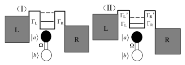
Figure 5: Schematics for a solid-state qubit measurement by SET. Model (I): the SET level is within the bias window for qubit state $|b\rangle$, but outside for state $|a\rangle$. Model (II): the SET level is between the Fermi levels for either $|b\rangle$ or $|a\rangle$, but with different couplings to the leads, i.e., $\Gamma_{L/R}$ for $|b\rangle$, and $\Gamma^{\prime}_{L/R}$ for $|a\rangle$.

As mentioned earlier for the QPC detector, a more implementable approach is continuous weak measurement rather than single-shot measurement. This type of measurement allows one to determine the ensemble average of detector and qubit states, and the qubit coherent oscillation is read out from the spectral density of the detector. In continuous weak measurement, an interesting generic result is the so-called Korotkov-Averin (K-A) bound, i.e., the signal-to-noise ratio (SNR) bounded by a fundamental limit of “4” K-A01 , which can be broken only in cases such as when performing quantum nondemolition (QND) measurement Ave02 , adding quantum feedback control Wang07 , or using two detectors But06 . We consider continuous weak measurement of qubits using strongly responding SETs Wis06 ; Gur05 and show that, for both models in Refs. Wis06, and Gur05, , the SNR can violate the universal Korotkov-Averin bound AK .

The entire method of the qubit-SET measurement is described by the following Hamiltonian Wis06 ; Gur05 ; AK

$$H =H_{0}+H^{\prime}$$ (33a)

$$H_{0} =H_{S}+\sum_{\lambda=L,R}\epsilon_{\lambda k}d_{\lambda k}^{\dagger}d_{\lambda k}$$ (33b)

$$H_{S} =\sum_{j=a,b}E_{j}|j\rangle\langle j|+\Omega(|a\rangle\langle b|+|b\rangle\langle a|)+E_{c}a_{c}^{\dagger}a_{c}+Un_{a}n_{c}$$ (33c)

$$H^{\prime} =\sum_{\lambda=L,R;k}(\Omega_{\lambda k}a_{c}^{\dagger}d_{\lambda k}+{\rm H.c.})\equiv~{}a_{c}^{\dagger}(f_{cL}+f_{cR})+{\rm H.c.}$$ (33d)

For simplicity, we assumed spinless electrons. The system Hamiltonian, $H_{S}$, contains a qubit, SET central dot, and their Coulomb interaction (the $U$-term). For the qubit, we assumed that each dot has only one bound state, i.e., the logic states $|a\rangle$ and $|b\rangle$ with energies $E_{a}$ and $E_{b}$ and a coupling amplitude $\Omega$. $n_{a}$ is the number operator of qubit state $|a\rangle$, which is 1 for $|a\rangle$ being occupied and 0 otherwise. For the SET, $a_{c}^{\dagger}(a_{c})$ and $d_{\alpha k}^{\dagger}(d_{\alpha k})$ are the electron creation (annihilation) operators of the central dot and reservoirs, respectively. $n_{c}\equiv a_{c}^{\dagger}a_{c}$ is introduced as the number operator of the SET dot. Similar to previous work, we assumed that the SET works in the strong Coulomb-blockade regime, with only a single level $E_{c}$ involved in the measurement process. Finally, $H^{\prime}$ describes the tunnel coupling of the SET dot to the leads, with amplitude $\Omega_{\lambda k}$.

We consider the two models schematically shown in Fig. 5. In model (I), which was studied in Ref. Gur05, , the SET dot level is within the bias voltage if the qubit is in state $|b\rangle$, but is above the Fermi level when the qubit state is switched to $|a\rangle$. For state $|b\rangle$, a nonzero current $I_{b}$ flows through the SET; however, for state $|a\rangle$, the SET current $I_{a}$ is zero. Then, the qubit state can be discriminated from these different currents. In this model, the signal current $\Delta I\equiv|I_{b}-I_{a}|$ is twice the average current $\bar{I}\equiv(I_{b}+I_{a})/2$. Hence, it is not a weak response detector. In model (II), which illustrates the crossover from weak to strong responses, the SET dot level is always between the Fermi levels of the two leads for qubits either in state $|b\rangle$ or state $|a\rangle$, but with different coupling strengths to the leads, i.e., $\Gamma_{L(R)}$ and $\Gamma^{\prime}_{L(R)}$. We further parameterize the tunnel couplings as $\Gamma_{L}(\Gamma_{L}^{\prime})=(1\pm\xi)\bar{\Gamma}_{L}$, $\Gamma_{R}(\Gamma_{R}^{\prime})=(1\pm\zeta)\bar{\Gamma}_{R}$, and $\gamma=\bar{\Gamma}_{R}/\bar{\Gamma}_{L}$. Here, $\bar{\Gamma}_{L(R)}=(\Gamma_{L(R)}+\Gamma^{\prime}_{L(R)})/2$ denotes the average couplings, while $\xi$ and $\zeta$ characterize the response strength of the detector to qubits. In this context, we would like to mention that, usually, the analysis is restricted in the weak-response regime by assuming that $\xi\ll 1$ and $\zeta\ll 1$, except in Ref. Wis06, , where the quantum efficiency was investigated in the strong response regime using this model.

For the both models in Fig. 5, the states involved are $|1\rangle=|0a\rangle$, $|2\rangle=|0b\rangle$, $|3\rangle=|1a\rangle$, and $|4\rangle=|1b\rangle$. In this notation $|0(1)a(b)\rangle$ means that the SET dot is empty (occupied) and the qubit is in state $|a(b)\rangle$. Applying Eq. (11) to model (I) yields AK

$$\dot{\rho}^{(n_{R})}_{11}= i\Omega[\rho^{(n_{R})}_{12}-\rho^{(n_{R})}_{21}]+\Gamma_{L}\rho^{(n_{R})}_{33}+\Gamma_{R}\rho^{(n_{R}-1)}_{33}$$ (34a)

$$\dot{\rho}^{(n_{R})}_{22}= i\Omega[\rho^{(n_{R})}_{21}-\rho^{(n_{R})}_{12}]-\Gamma_{L}\rho^{(n_{R})}_{22}+\Gamma_{R}\rho^{(n_{R}-1)}_{44}$$ (34b)

$$\dot{\rho}^{(n_{R})}_{12}= -i\epsilon\rho^{(n_{R})}_{12}+i\Omega[\rho^{(n_{R})}_{11}-\rho^{(n_{R})}_{22}]-\frac{\Gamma_{L}}{2}\rho^{(n_{R})}_{12}$$

$$+\frac{\Gamma_{L}}{2}\rho^{(n_{R})}_{34}+\Gamma_{R}\rho^{(n_{R}-1)}_{34}$$ (34c)

$$\dot{\rho}^{(n_{R})}_{33}= i\Omega[\rho^{(n_{R})}_{34}-\rho^{(n_{R})}_{43}]-(\Gamma_{R}+\Gamma_{L})\rho^{(n_{R})}_{33}$$ (34d)

$$\dot{\rho}^{(n_{R})}_{44}= i\Omega[\rho^{(n_{R})}_{43}-\rho^{(n_{R})}_{34}]+\Gamma_{L}\rho^{(n_{R})}_{22}-\Gamma_{R}\rho^{(n_{R})}_{44}$$ (34e)

$$\dot{\rho}^{(n_{R})}_{34}= -i(\epsilon+U)\rho^{(n_{R})}_{34}+i\Omega[\rho^{(n_{R})}_{33}-\rho^{(n_{R})}_{44}]$$

$$+\frac{\Gamma_{L}}{2}\rho^{(n_{R})}_{12}-(\Gamma_{R}+\frac{\Gamma_{L}}{2})\rho^{(n_{R})}_{34}$$ (34f)

Here, $\epsilon=E_{a}-E_{b}$ and $\Gamma_{L/R}=2\pi|\Omega_{L/R}|^{2}g_{L/R}$, where $g_{L/R}$ is the density of states of the SET leads. For simplicity, the assumption of the wide-band limit implies $\Omega_{L/R}\equiv\Omega_{L/Rk}$, and makes $\Gamma_{L/R}$ energy independent. In addition, low temperature conditions and $U\gg\Omega$ were assumed to further simplify the equations. Similarly, for model (II), we have AK

$$\dot{\rho}^{(n_{R})}_{11}= i\Omega[\rho^{(n_{R})}_{12}-\rho^{(n_{R})}_{21}]-\Gamma_{L}^{\prime}\rho^{(n_{R})}_{11}+\Gamma_{R}^{\prime}\rho^{(n_{R}-1)}_{33}$$ (35a)

$$\dot{\rho}^{(n_{R})}_{22}= i\Omega[\rho^{(n_{R})}_{21}-\rho^{(n_{R})}_{12}]-\Gamma_{L}\rho^{(n_{R})}_{22}+\Gamma_{R}\rho^{(n_{R}-1)}_{44}$$ (35b)

$$\dot{\rho}^{(n_{R})}_{12}= -i\epsilon\rho^{(n_{R})}_{12}+i\Omega[\rho^{(n_{R})}_{11}-\rho^{(n_{R})}_{22}]$$

$$-\frac{\Gamma_{L}+\Gamma_{L}^{\prime}}{2}\rho^{(n_{R})}_{12}+\frac{\Gamma_{R}+\Gamma_{R}^{\prime}}{2}\rho^{(n_{R}-1)}_{34}$$ (35c)

$$\dot{\rho}^{(n_{R})}_{33}= i\Omega[\rho^{(n_{R})}_{34}-\rho^{(n_{R})}_{43}]+\Gamma_{L}^{\prime}\rho^{(n_{R})}_{11}-\Gamma_{R}^{\prime}\rho^{(n_{R})}_{33}$$ (35d)

$$\dot{\rho}^{(n_{R})}_{44}= i\Omega[\rho^{(n_{R})}_{43}-\rho^{(n_{R})}_{34}]+\Gamma_{L}\rho^{(n_{R})}_{22}-\Gamma_{R}\rho^{(n_{R})}_{44}$$ (35e)

$$\dot{\rho}^{(n_{R})}_{34}= -i(\epsilon+U)\rho^{(n_{R})}_{34}+i\Omega[\rho^{(n_{R})}_{33}-\rho^{(n_{R})}_{44}]$$

$$+\frac{\Gamma_{L}+\Gamma_{L}^{\prime}}{2}\rho^{(n_{R})}_{12}-\frac{\Gamma_{R}+\Gamma_{R}^{\prime}}{2}\rho^{(n_{R})}_{34}$$ (35f)

Except for the specific conditions of model (II), the other parameters are the same as those for model (I) (as mentioned above).

By applying the $n$-ME formulation in Eqs. (18)-(26), we can straightforwardly calculate the output power spectrum for both set-ups considered here. As for qubit measurement using a QPC detector, the signal of the qubit oscillations is manifested as a peak in the noise spectrum at frequency $2\Omega$, while the measurement effectiveness is characterized by the SNR, i.e., the peak-to-pedestal ratio. We denote the noise pedestal by $S_{p}$, and obtain it from $S(\omega\rightarrow\infty)$. In Fig. 6, we show the dependence of the SNR on the detector’s configuration symmetries.

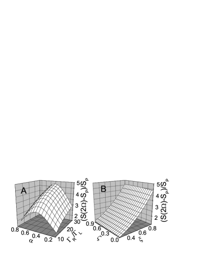
Figure 6: Signal-to-noise ratio: (A) for model (I), and (B) for model (II). For model (I), we take $\Gamma_{L}=\Gamma$ as energy unit and assume that $\mu_{L(R)}=\pm 50\Gamma$, $\Omega=2\Gamma$ and $U=80\Gamma$. For model (II), we take $\bar{\Gamma}_{L}=\bar{\Gamma}$ as energy unit and assume that $\Omega=\bar{\Gamma}$, $U=50\bar{\Gamma}$, $\bar{\Gamma}_{R}=30\bar{\Gamma}$, and $\alpha=\beta=1/2$. Zero temperature and $E_{a}=E_{b}$ are assumed.

Figure 7: Signal-to-noise ratio versus tunnel-coupling asymmetry, $\Gamma_{R}/\Gamma_{L}$ for model (I), and $\bar{\Gamma}_{R}/\bar{\Gamma}_{L}$ for model (II). In (A) the solid and dashed lines are the result in the presence of cross correlation, while the dotted and dot-dashed lines are the result after removing it. In (B) the mere cross correlation is plotted. $S_{p}$ is the pedestal noise of the entire circuit current. $\xi=\zeta=0.9$, other parameters are the same as in Fig. 6.

Figure 8: Spectral density of the cross-correlation scaled by its own pedestal, which is defined here at twice the Rabi frequency of the qubit oscillations. Parameters for model (I) in (A): $\Gamma_{L}=0.05\Gamma$, $\Gamma_{R}=0.5\Gamma$, and $\Omega=5\Gamma$. Parameters for model (II) in (B): $\bar{\Gamma}_{L}=0.05\Gamma$, $\bar{\Gamma}_{R}=0.5\Gamma$, $\Omega=5\Gamma$, and $\xi=\zeta=0.9$. In this plot we take $\Gamma$ as the energy unit. Other conventions are the same as in Fig. 6.

The result of model (I) is shown in Fig. 6(A), where we see that both the tunnel- and capacitive-coupling symmetries crucially affect the measurement effectiveness. The tunnel coupling asymmetry effect $\Gamma_{R}/\Gamma_{L}$ is due to the fact that with the increase of $\Gamma_{R}/\Gamma_{L}$, the interaction time between the detector electron and the qubit is decreased. Thus, the detector’s back-action is reduced and the SNR is enhanced Gur05 . For the effect of capacitive coupling, its degree of asymmetry affects the contribution weight of the cross-correlation between $I_{L}(t)$ and $I_{R}(t)$ to the entire circuit noise. Specifically, the cross-correlation has a more important contribution for more symmetric coupling, as shown in Fig. 6(A) by the $\alpha$-dependence. This is because, as we shall demonstrate below, the cross-correlation has a much higher peak-to-pedestal ratio than the auto-correlation.

An unexpected feature observed in Fig. 6(A) is that under proper conditions, i.e., for symmetric capacitive coupling and strongly asymmetric tunnel coupling, the SNR can exceed “4”, which is the upper bound quantum mechanically limited on any linear response detectors K-A01 . However, whether this upper bound is applicable to nonlinear response detector is unclear in priori, since, in this case, the linear response relation between the current and qubit state breaks down. Hence, the subsequent Cauchy-Schwartz-inequality-based argument leading to the upper bound of “4” is not valid But06 .

To support the above theory, we further study model (II). The result is presented in Fig. 6(B). As explained in the model description, the parameters $\xi$ and $\zeta$ characterize, respectively, the left and right tunnel-coupling responses to the qubit states. Fig. 6(B) shows an asymmetric tunnel coupling detector, with $\gamma\equiv\bar{\Gamma}_{R}/\bar{\Gamma}_{L}=30$, which can lead to higher SNR, because of the weaker back-action from the detector, similar to that for model (I). Here, we find that the SNR is insensitive to the right junction response $\zeta$, but sensitive to the left one $\xi$. Again, in this model, we observe that the SNR can violate the K-A bound “4” in the strong response regime.

We present further explanation of the violation of the K-A bound. Since $I(t)=\alpha I_{L}(t)+\beta I_{R}(t)$, the current correlator $\langle I(t)I(0)\rangle$ contains the component $S_{LR}(t)\equiv\langle I_{L}(t)I_{R}(0)+I_{R}(t)I_{L}(0)\rangle$, i.e., the cross-correlation. In addition, in the previous results, we see that for more symmetric capacitive coupling, the SNR is larger, and reaches a maximum at $\alpha=\beta=1/2$. This feature indicates that the cross-correlation can enhance the SNR. Indeed, for the SET detector, both the left and right junction currents ($I_{L}$ and $I_{R}$) contain information of the qubit state; hence, their “signal” parts are correlated. This leads to a heuristic opinion that views the two junctions as two detectors, like in the scheme of qubit measurement using two point contacts proposed recently by Jordan and Büttiker But06 , where they found that the SNR of the cross-correlation can strongly violate the K-A bound, because of the negligibly small pedestal of the cross noise. In our case, since $I_{L}(t)$ and $I_{R}(t)$ are subject to a constraint from charge conservation, the cross noise background of $I_{L}(t)$ and $I_{R}(t)$ does not vanish in principle, unlike for the two independent QPC detectors But06 . Nevertheless, the pedestal of the cross noise of the SET is much smaller than that of the auto-correlation, which leads to an enhanced SNR in the spectral density of the total circuit current and to the violation of the K-A bound, as clearly shown in Fig. 7(A). For comparative purposes, in Fig. 7(B), we plot the SNR of the cross-correlation, scaled by the noise pedestal $S_{p}$ of the circuit current.

In Fig. 8, the spectral density of the cross-correlation, scaled by its own noise pedestal, is shown representatively. As mentioned above, since the cross noise pedestal is negligibly small at a high frequency limit, we artificially (but more physically in some sense) define the pedestal at a finite frequency, e.g., twice the qubit oscillation frequency. Obviously, the large SNR of the cross-correlation drastically violates the K-A bound. This result indicates that for qubit measurement using an SET, one can explore the cross-correlation, rather than the auto-correlation, as a probe of coherent oscillations. In practice, such scheme is simpler than the technique of QND measurement Ave02 , and holds the most advantages of SET over QPC.

IV Application to Quantum Transport

We illustrate

the application of the $n$-ME approach to quantum transport by first using a single-level quantum dot to show the simple results of the $n$-resolved master equation and then considering two more interesting examples.

IV.1 Single-Level Quantum Dot

For transport through

a single-level ($E_{0}$) quantum dot, under wide-band approximation, the reservoir correlation functions can be expressed as $C_{\alpha}^{(\pm)}(t-\tau)=|t_{\alpha}|^{2}\sum_{k}e^{\pm i\epsilon_{k}(t-\tau)}n^{(\pm)}_{\alpha}(\epsilon_{k})$, where $n^{(+)}_{\alpha}(\epsilon_{k})=n_{\alpha}(\epsilon_{k})$ is the Fermi distribution function and $n^{(-)}_{\alpha}(\epsilon_{k})=1-n_{\alpha}(\epsilon_{k})$. Then, the spectral functions are obtained as

$$A_{\alpha}^{(\pm)}=C_{\alpha}^{(\pm)}(\pm{\cal L})a=\Gamma_{\alpha}n^{(\pm)}_{\alpha}(E_{0})a\,.$$ (36)

Here, $\Gamma_{\alpha}=2\pi g_{\alpha}|t_{\alpha}|^{2}$, where $g_{\alpha}$ is the density of states of the “$\alpha$” lead. In the special case of zero temperature and a large bias voltage $\mu_{L}\gg E_{0}\gg\mu_{R}$, we have $A^{(+)}_{L}=\Gamma_{L}a$, $A^{(-)}_{L}=0$  , $A^{(-)}_{R}=\Gamma_{R}a$, and $A^{(+)}_{R}=0$  . Substituting these into Eq. (11) yields

$$\dot{\rho}^{(n)} = -i{\cal L}\rho^{(n)}-\frac{1}{2}\left\{[\Gamma_{R}a^{\dagger}a\rho^{(n)}+\Gamma_{L}\rho^{(n)}aa^{\dagger}\right.$$ (37)

$$\left.-\Gamma_{L}a^{\dagger}\rho^{(n)}a-\Gamma_{R}a\rho^{(n-1)}a^{\dagger}]+{\rm H.c.}\right\}\,.$$

Choosing the empty state $|0\rangle$ and the occupied one $|1\rangle$, we obtain

$$\dot{\rho}^{(n)}_{00} = -\Gamma_{L}\rho^{(n)}_{00}+\Gamma_{R}\rho^{(n-1)}_{11}\,,$$

$$\dot{\rho}^{(n)}_{11} = -\Gamma_{R}\rho^{(n)}_{11}+\Gamma_{L}\rho^{(n)}_{00}\,.$$ (38)

This is the result derived by Gurvitz et al under the limits mentioned above Gur96b . Applying the above $n$-ME, one can easily perform all the transport studies outlined in Sec. II.

IV.2 Parallel Double Dots

The system of two quantum dots

coupled in parallel to two reservoirs has attracted a great deal of attention as a realization of a mesoscopic Aharonov–Bohm interferometer holl ; chen ; sigr . Indeed, such a system pierced by an external magnetic field, as shown in Fig. 9, is an interference device whose transmission can be tuned by varying the magnetic field. In the absence of the interdot electron–electron interaction, the interference effects in the resonant current through this system are quite transparent. This is not the case, however, for interacting electrons gefen ; neder .

We consider a strong interdot electron-electron repulsion—a Coulomb blockade. While the two dots may be occupied simultaneously in the noninteracting model, the Coulomb blockade prevents this. At first, one might not expect that this repulsion could dramatically modify the resonant current’s dependence on the magnetic field. We find, however, that the resonant current is completely blocked for any value of the magnetic flux except for integer multiples of the flux quantum ($\Phi_{0}=h/e$) DD-1 . This striking effect goes far beyond our simple expectations.

Consider a double dot (DD) connected in parallel to two reservoirs, as shown in Fig. 9. For simplicity, we consider spinless electrons. We also assume that each of the dots contains only one level, $E_{1}$ and $E_{2}$. In the presence of a magnetic field, the system can be described by the following tunneling Hamiltonian DD-1 ,

$$H=H_{0}+H_{T}+\sum_{\mu=1,2}E_{\mu}d_{\mu}^{\dagger}d_{\mu}+Ud_{1}^{\dagger}d_{1}d_{2}^{\dagger}d_{2}\,.$$ (39)

Here, the first term, $H_{0}=\sum_{k}[E_{kL}a_{kL}^{\dagger}a_{kL}+E_{kR}a_{kR}^{\dagger}a_{kR}]$, describes the reservoirs and $H_{T}$ describes their coupling to the dots,

$$H_{T}=\sum_{\mu,k}\Big{(}t_{\mu L}d_{\mu}^{\dagger}a_{kL}+t_{\mu R}a_{kR}^{\dagger}d_{\mu}\Big{)}+{\rm H.c.}\,,$$ (40)

where $\mu=1,2$ and $a_{kL}^{\dagger}$ and $a_{kR}^{\dagger}$ are the creation operators for the electrons in the reservoirs while $d_{1,2}^{\dagger}$ is the creation operator for the DD. The last term in Eq. (39) describes the interdot repulsion. We assume that there is no direct transmission between the dots and that the couplings of the dots to the leads, $t_{\mu L(R)}$, are independent of energy. In the absence of a magnetic field, one can always choose the gauge in such a way that all couplings are real. In the presence of a magnetic flux $\Phi$, however, the tunneling amplitudes between the dots and the reservoirs are generally complex. We obtain $t_{\mu L(R)}={\bar{t}}_{\mu L(R)}e^{i\phi_{\mu L(R)}}$, where $\bar{t}_{\mu L(R)}$ is the coupling without the magnetic field. The phases around the closed circle are constrained to satisfy $\phi_{1L}+\phi_{1R}-\phi_{2L}-\phi_{2R}=\phi$, where $\phi\equiv 2\pi\Phi/\Phi_{0}$.

Figure 9: Resonant tunneling through two parallel dots pierced by the magnetic flux $\Phi$.

Let the initial state of the system correspond to filling the left and right reservoirs at zero temperature with electrons up to the Fermi energies $\mu_{L}$ and $\mu_{R}$, respectively. In the case of large bias, $|\mu_{L,R}-E_{1,2}|\gg\Gamma$, applying either an exact single-particle wavefunction method or the ME approach for non-interacting case, we find a simple expression for the total current DD-1

$$I(\phi)=I_{0}{\Delta^{2}+\Gamma_{L}\Gamma_{R}\sin^{2}\phi\over\Delta^{2}+\Gamma_{L}\Gamma_{R}\sin^{2}{\displaystyle\phi\over\displaystyle 2}\,}\,,$$ (41)

where $\Delta=E_{1}-E_{2}$ is the offset of the dot levels, and $I_{0}=2\Gamma_{L}\Gamma_{R}/\Gamma$ is the current for non-interacting electrons in the absence of the magnetic filed, with $\Gamma_{L(R)}=2\pi D_{L(R)}|\bar{t}_{L(R)}|^{2}$ and $D_{L(R)}$ is the density of states of the leads. The $\phi$-dependence in Eq.(41) is an example of the Aharonov–Bohm effect.

Next, we detail the study for interacting dots in the Coulomb blockade case, $E_{1,2}+U\gg\mu_{L}$, which excludes the states corresponding to a simultaneous occupation of the two dots. In this case, the Hilbert space of the DD state is reduced to $|0\rangle\equiv|00\rangle$, $|1\rangle\equiv|10\rangle$, and $|2\rangle\equiv|01\rangle$, where $|10\rangle$ means the upper dot occupied and the lower dot unoccupied, and other states have similar interpretations. Applying Eq. (11), we obtain DD-2

$$\dot{\rho}^{(n)}_{00}=-2\Gamma_{L}\rho_{00}^{(n)}+\Gamma_{R}\rho_{11}^{(n-1)}+\Gamma_{R}\rho_{22}^{(n-1)}+e^{i\left(\phi_{\text{R1}}-\phi_{\text{R2}}\right)}\Gamma_{R}\rho_{12}^{(n-1)}+e^{i\left(\phi_{\text{R2}}-\phi_{\text{R1}}\right)}\Gamma_{R}\rho_{21}^{(n-1)}$$ (42a)

$$\dot{\rho}_{11}^{(n)}=\Gamma_{L}\rho_{00}^{(n)}-\Gamma_{R}\rho_{11}^{(n)}-\frac{1}{2}e^{i\left(\phi_{\text{R1}}-\phi_{\text{R2}}\right)}\Gamma_{R}\rho_{12}^{(n)}-\frac{1}{2}e^{i\left(\phi_{\text{R2}}-\phi_{\text{R1}}\right)}\Gamma_{R}\rho_{21}^{(n)}$$ (42b)

$$\dot{\rho}_{22}^{(n)}=\Gamma_{L}\rho_{00}^{(n)}-\Gamma_{R}\rho_{22}^{(n)}-\frac{1}{2}e^{i\left(\phi_{\text{R1}}-\phi_{\text{R2}}\right)}\Gamma_{R}\rho_{12}^{(n)}-\frac{1}{2}e^{i\left(\phi_{\text{R2}}-\phi_{\text{R1}}\right)}\Gamma_{R}\rho_{21}^{(n)}$$ (42c)

$$\dot{\rho}_{12}^{(n)}=e^{i\left(\phi_{\text{L1}}-\phi_{\text{L2}}\right)}\Gamma_{L}\rho_{00}^{(n)}-\frac{1}{2}e^{i\left(\phi_{\text{R2}}-\phi_{\text{R1}}\right)}\Gamma_{R}\rho_{11}^{(n)}-\frac{1}{2}e^{i\left(\phi_{\text{R2}}-\phi_{\text{R1}}\right)}\Gamma_{R}\rho_{22}^{(n)}-(\Gamma_{R}+i\Delta)\rho_{12}^{(n)}$$ (42d)

$$\dot{\rho}_{21}^{(n)}=e^{i\left(\phi_{\text{L2}}-\phi_{\text{L1}}\right)}\Gamma_{L}\rho_{00}^{(n)}-\frac{1}{2}e^{i\left(\phi_{\text{R1}}-\phi_{\text{R2}}\right)}\Gamma_{R}\rho_{11}^{(n)}-\frac{1}{2}e^{i\left(\phi_{\text{R1}}-\phi_{\text{R2}}\right)}\Gamma_{R}\rho_{22}^{(n)}-(\Gamma_{R}-i\Delta)\rho_{21}^{(n)}$$ (42e)

Owing to the neglected spin degrees of freedom in constructing the Hilbert space, as a compensation, here we have replaced $\Gamma_{L}$ with $2\Gamma_{L}$ to equivalently restore its effect.

Applying the $n$-ME approach, we obtain the total current in the steady-state limit DD-1 ; DD-2

$$I(\phi)=I_{C}{\Delta^{2}\over\Delta^{2}+I_{C}\left(2\Gamma_{R}\sin^{2}{\displaystyle\phi\over\displaystyle 2}-\Delta\sin\phi\right)}\,,$$ (43)

where $I_{C}=2\Gamma_{L}\Gamma_{R}/(2\Gamma_{L}+\Gamma_{R})$ is the total current (with the Coulomb blockade) in the absence of the magnetic field. Let us compare Eq. (43) with Eq. (41) for the noninteracting case. We find that for $\Delta\not=0$ both currents display the Aharonov–Bohm oscillations. However, their behavior is drastically different when $\Delta\to 0$. The resonant current for the noninteracting electrons keeps oscillating with the magnetic field, while in the case of the Coulomb blockade, the current becomes non-analytic in $\phi$. From Eq. (43), we can easily obtain that $I=I_{C}$ for $\phi=2\pi n$, where $n=\Phi/\Phi_{0}$ is an integer, but $I=0$ for any other value of $\Phi$. Such an unexpected “switching” behavior of the electron current in the magnetic field represents a non-trivial interplay of the Coulomb blockade and quantum interference.

For understanding the switching phenomenon, it is desirable to disentangle these two effects via a state basis transformation, by defining new basis DD states, $d^{\dagger}_{\mu}|0\rangle\to\tilde{d}^{\dagger}_{\mu}|0\rangle$, chosen such that $\tilde{d}^{\dagger}_{2}|0\rangle$ is not coupled to the right reservoir, i.e., $t_{2R}\to\tilde{t}_{2R}=0$, then the current would flow only through the state $\tilde{d}_{1}^{\dagger}|0\rangle$. This can be realized using the unitary transformation DD-1 ; DD-2

$$\left(\begin{array}[]{c}\widetilde{d}_{1}\\ \widetilde{d}_{2}\end{array}\right)={1\over{\cal N}}\left(\begin{array}[]{cc}t_{1R}&t_{2R}\\ -t^{*}_{2R}&t^{*}_{1R}\end{array}\right)\left(\begin{array}[]{c}d_{1}\\ d_{2}\end{array}\right),$$ (50)

where ${\cal N}=(\bar{t}_{1R}^{2}+\bar{t}_{2R}^{2})^{1/2}$, which indeed results in $\widetilde{t}_{2R}=0$. In addition, the coupling of $\widetilde{d}^{\dagger}_{2}|0\rangle$ to the left lead reads

$$\widetilde{t}_{2L}(\phi)=-e^{i(\phi_{2L}-\phi_{1R})}(\bar{t}_{1L}\bar{t}_{2R}\,e^{i\phi}-\bar{t}_{2L}\bar{t}_{1R})/{\cal N}.$$ (51)

It follows from this expression that $\widetilde{t}_{2L}=0$ for $\phi=2n\pi$ provided that $\bar{t}_{1L}/\bar{t}_{2L}=\bar{t}_{1R}/\bar{t}_{2R}$, or for $\phi=(2n+1)\pi$ if $\bar{t}_{1L}/\bar{t}_{2L}=-\bar{t}_{1R}/\bar{t}_{2R}$. Obviously, for noninteracting DD, $\widetilde{d}^{\dagger}_{2}|0\rangle$ has no contribution to current, while $\widetilde{d}^{\dagger}_{1}|0\rangle$ carries a magnetic-flux modulated current. In the case of inter-dot Coulomb blockade, however, the coupling of $\widetilde{d}^{\dagger}_{2}|0\rangle$ to the left lead is zero, which is of crucial importance. If $\widetilde{t}_{2L}\neq 0$, then the state $\widetilde{d}_{1}^{\dagger}|0\rangle$, carrying the current, will be blocked by the inter-dot Coulomb repulsion. As a result, the total current vanishes. However, if the state $\widetilde{d}_{2}^{\dagger}|0\rangle$ is decoupled from both leads, it remains unoccupied, so that the current can flow through the state $\widetilde{d}_{1}^{\dagger}|0\rangle$. As shown above, this takes place precisely for $\bar{t}_{1L}/\bar{t}_{2L}=\pm\,\bar{t}_{1R}/\bar{t}_{2R}$. If this condition is not fulfilled, the current is always zero, even for $\phi=2\pi n$.

Below we consider further the current fluctuations. The shot-noise spectrum can be conveniently calculated using the $n$-ME and the MacDonald’s formula. Noticeably, for the present Coulomb blockade DD interferometer, we find that the zero-frequency shot noise can be highly super-Poissonian, and can even become divergent as $\Delta\rightarrow 0$. For the coherent DD interferometer, analytical result of the frequency-dependent noise can be obtained as DD-2

$$S(\omega)=\frac{8\Gamma_{L}\Gamma_{R}[2\Gamma_{L}\Gamma_{R}\Delta^{2}-\Delta^{4}+3\Delta^{2}\omega^{2}-2\omega^{2}(\Gamma^{2}_{R}+\omega^{2})]\bar{I}}{[(2\Gamma_{L}+\Gamma_{R})\Delta^{2}-(2\Gamma_{L}+3\Gamma_{R})\omega^{2}]^{2}+\omega^{2}(2\Gamma_{L}\Gamma_{R}+2\Gamma^{2}_{R}+\Delta^{2}-\omega^{2})^{2}}+2\bar{I}~{}.$$ (52)

Here, we have assumed $\phi=2\pi n$. At zero frequency limit, the Fano factor can be given as

$$F\equiv\frac{S(0)}{2\bar{I}}=\frac{8\Gamma^{2}_{L}\Gamma^{2}_{R}+(4\Gamma^{2}_{L}+\Gamma^{2}_{R})\Delta^{2}}{(2\Gamma_{L}+\Gamma_{R})^{2}\Delta^{2}}.$$ (53)

Noticeably, as $\Delta\rightarrow 0$, it becomes divergent! Note that this divergence is not caused by the average current $\bar{I}$, but by the zero-frequency noise itself. In addition, from Eq. (52), we find that the limiting order of $\Delta\rightarrow 0$ and $\omega\rightarrow 0$, would lead to different results i.e., if $\Delta\rightarrow 0$, then $\omega\rightarrow 0$, the result can be given as

$$F=\frac{\Gamma^{2}_{L}+\Gamma^{2}_{R}}{(\Gamma_{L}+\Gamma_{R})^{2}},$$ (54)

which is finite and coincides with the Fano factor of the single-level transport Li053 . The limiting order leading to Eq. (54), which implies that we are considering the noise for aligned DD levels. In this case, as constructed above, see Eq. (50) and Fig. 10(a), the two transformed dot-states are decoupled to each other, and one of them is also decoupled to both leads if $\phi=2\pi n$. As a result, equivalently, the transport is through a single channel, leading to the Fano factor Eq. (54).

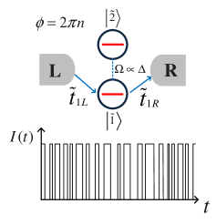
Figure 10: Schematic interpretation for the noise divergence. Upper panel: Effective coupling of the DD to the leads and between the dots, in the representation of transformed DD states, i.e., $|\tilde{1}\rangle\equiv\tilde{d}^{\dagger}_{1}|0\rangle$ and $|\tilde{2}\rangle\equiv\tilde{d}^{\dagger}_{2}|0\rangle$. Lower panel: Coarse-grained temporal current, with a telegraphic noise nature which causes divergence of the zero-frequency noise when $\Delta\rightarrow 0$ .

However, for $\Delta\rightarrow 0$ but $\neq 0$, the situation is subtly different. In this case, the two transformed states are weakly coupled, with a strength $\propto\Delta$. Thus, the transporting electron on state $\tilde{d}_{1}^{\dagger}|0\rangle$ can occasionally tunnel to $\tilde{d}_{2}^{\dagger}|0\rangle$, which is disconnected to both leads, and its occupation will block the current until the electron tunnels back to $\tilde{d}_{1}^{\dagger}|0\rangle$ and arrives at the right lead. Typically, this strong bunching behavior, induced by the interplay of Coulomb interaction and quantum interference, is well characterized by a profound super-Poissonian statistics. In Fig. 10(b), the coarse-grained temporal current with a telegraphic noise nature is plotted schematically. We observe that, as $\Delta\rightarrow 0$, the current switching would become extremely slow, leading to very long time ($\sim 1/\Delta$) correlation between the transport electrons. This long-time-scale fluctuation, or equivalently, the low frequency component filtered out from the current, which causes divergence of the shot noise as $\Delta\rightarrow 0$. This is similar, in a certain sense, to the well known $1/f$ noise, which goes to divergence as $f\rightarrow 0$.

IV.3 Probe of Majorana Fermion

In this subsection, we apply the $n$-ME approach

to analysis for a possible probe of the Majorana fermions MF-1 ; MF-2 ; MF-3 . The Majorana fermions, proposed in 1937 by Majorana MF37 , are exotic particles since each Majorana fermion is its own antiparticle Wil0910 . The search for Majorana fermions in solid states, as emerged quasiparticles (elementary excitations), has been attracting a great deal of attention Kit01 ; Fu08 ; Ore10 ; Sau10 ; Lut10 ; Ali10 ; Sau12 . As a real example, an effective $p$-wave superconductor can be realized using a semiconductor nanowire with Rashba spin-orbit interaction and Zeeman splitting, and in proximity to an $s$-wave superconductor Ore10 ; Sau10 ; Sau12 . Of crucial importance is then a full experimental demonstration of the Majorana fermion in solid states Kou12 .

Therefore, let us consider the system in Fig. 11. The setup describes transport through a semiconductor quantum dot (QD), while the QD is tunnel-coupled to a semiconductor nanowire on an $s$-wave superconductor Kou12 . It was found in Ref. Liu11 that the Majorana bound state (MBS), emerged at the end of the nanowire, will dramatically influence the zero-bias linear-response conductance through the quantum dot, as a result of the modified static spectral property (the effective density-of-states) of the QD level. In the following section, going beyond linear response, we consider transport through the quantum dot under finite bias voltage and pay particular attention to the Majorana’s dynamic aspect MF-1 ; MF-2 ; MF-3 . While a subtraction of the source and drain currents can expose certain features of the Majorana fermion MF-1 , below we show that the more unique properties can be identified from the shot noise MF-1 ; MF-2 , via a spectral dip together with a pronounced zero-frequency noise enhancement effect.

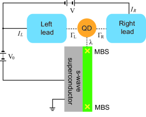
Figure 11: Schematic setup for detecting Majorana fermion by transport through a semiconductor quantum dot (QD), while the QD is coupled to a semiconductor nanowire which is in contact with an $s$-wave superconductor. Under appropriate conditions a pair of Majorana bound states (MBS) is anticipated to emerge at the ends of the nanowire.

Combining a strong Rashba spin-orbit interaction and the Zeeman splitting, it was shown that the proximity-effect-induced $s$-wave superconductivity in the nanowire can support electron-hole quasiparticle excitations of Majorana bound states (MBS) at the ends of the nanowire Ore10 ; Sau10 ; Sau12 . Since the Zeeman splitting should be large enough in order to drive the wire into a topological superconducting phase, we can assume it much larger than the transport bias voltage, the dot-wire coupling energy, and the dot tunneling rates with the leads. In this case, we can model the QD by a single resonant level and treat the electron as spinless particle. Accordingly, the entire system can be modeled using $H=H_{\rm Leads}+H_{\rm sys}+H_{T}$. $H_{\rm Leads}=\sum_{\alpha=L,R}\sum_{k}\varepsilon_{\alpha k}c^{\dagger}_{\alpha k}c_{\alpha k}$ describes the normal metallic leads; $H_{T}=\sum_{\alpha=L,R}\sum_{k}t_{\alpha k}dc^{\dagger}_{\alpha k}+{\rm H.c.}$ is for the tunneling between the leads and the dot; and the low-energy effective Hamiltonian for the central system is given as MF-1 ; MF-2

$$H_{\rm sys}=\epsilon_{D}d^{\dagger}d+\frac{i}{2}\epsilon_{M}\gamma_{1}\gamma_{2}+(\lambda d-\lambda^{*}d^{\dagger})\gamma_{1}.$$ (55)

Here, $c^{\dagger}_{\alpha k}(c_{\alpha k})$ and $d^{\dagger}(d)$ are the electron creation (annihilation) operators of the leads and the dot, respectively, with corresponding energies of $\varepsilon_{\alpha k}$ and $\epsilon_{D}$. Particularly, in Eq. (55), the second term describes the paired MBSs generated at the ends of the nanowire and coupled to each other by an energy $\epsilon_{M}\sim e^{-l/\xi}$, where $l$ is the wire length and $\xi$ is the superconducting coherent length. The last term in Eq. (55) describes the tunnel coupling between the dot and the left MBS. For spinless dot level, we can choose a real constant $\lambda$, while in general $\lambda$ has a phase factor associated with the spin direction.

To solve the transport problem associated with the Hamiltonian Eq. (55), it is convenient to switch from the Majorana representation to the regular fermion representation, through the exact transformation $\gamma_{1}=f^{\dagger}+f$ and $\gamma_{2}=i(f^{\dagger}-f)$. $f$ is the regular fermion operator, satisfying the anti-commutative relation $\{f,f^{\dagger}\}=1$. Accordingly, we rewrite $H_{\rm sys}$ as MF-1 ; MF-2

$$H_{\rm sys}=\epsilon_{D}d^{\dagger}d+\epsilon_{M}\left(f^{\dagger}f-\frac{1}{2}\right)+\lambda(d-d^{\dagger})(f^{\dagger}+f).$$ (56)

For the convenience of the latter discussion, we rearrange the tunnel coupling term in Eq. (56) as $H_{1}=(\lambda f^{\dagger}d+\lambda_{1}f^{\dagger}d^{\dagger})+{\rm H.c.}$, where $\lambda_{1}=\lambda$ or $0$ corresponds to the dot coupling to the MBS or to a regular fermion bound state. In the transformed representation, the basis states of the central system are given by ${\left|n_{d}n_{f}\right\rangle}$, where $n_{d}$ and $n_{f}$ can take the value of 0 or 1, so that we have four basis states $\{{\left|00\right\rangle},{\left|10\right\rangle},{\left|01\right\rangle},{\left|11\right\rangle}\}$.

Rather than the linear response Liu11 , we consider transport through the quantum dot under finite bias voltage. Associated with the voltage setup in Fig. 11, the chemical potentials of the two leads are, $\mu_{L}=eV_{0}$ and $\mu_{R}=e(V_{0}-V)$. The so-called large bias limit indicates that $|\mu_{L(R)}-\epsilon_{D}|$ is much larger than the dot-level’s broadening. In this case, the dot level is deeply embedded into the voltage window and the temperature effect is negligible in calculating the transport currents. Moreover, this bias regime allows us to apply the Born-Markov ME. Its particle-number-resolved version is given as MF-1

$$\dot{\rho}^{(n)} \!\!=\!\! -i{\cal L}\rho^{(n)}\!-\!\frac{\Gamma_{L}}{2}\left(dd^{\dagger}\rho^{(n)}+\rho^{(n)}dd^{\dagger}-2d^{\dagger}\rho^{(n)}d\right)$$ (57)

$$-\frac{\Gamma_{R}}{2}\left(d^{\dagger}d\rho^{(n)}+\rho^{(n)}d^{\dagger}d-2d\rho^{(n-1)}d^{\dagger}\right),$$

where “$n$” represents the electron number transferred through the central system, and $\rho^{(n)}$ satisfies the condition $\sum_{n=0}^{\infty}\rho^{(n)}(t)=\rho(t)$. Here, we introduced the Liouvillian superoperator as ${\cal L}\rho\equiv[H_{\rm sys},\rho]$, and the tunneling rate as $\Gamma_{\alpha}=2\pi g_{\alpha}|t_{\alpha}|^{2}$, where $g_{\alpha}$ is the density-of-states of the lead $\alpha$ ($L$ or $R$). Corresponding to Eq. (57), the unconditional Lindblad ME is given as $\dot{\rho}=-i{\cal L}\rho+\Gamma_{L}{\cal D}[d^{\dagger}]\rho+\Gamma_{R}{\cal D}[d]\rho$, where ${\cal D}[A]\rho\equiv A\rho A^{\dagger}-\frac{1}{2}\{A^{\dagger}A,\rho\}$.

Shot Noise.— Below we focus our interest on the shot noise spectrum, which beyond the steady-state current, reflects the dynamic aspect of the central system. Specifically, we consider the current correlator $S_{\alpha}(t)=\frac{1}{2}\langle\{\delta I_{\alpha}(t),\delta I_{\alpha}(0)\}\rangle$, where $\alpha=L$ and $R$ and $\delta I_{\alpha}(t)=I_{\alpha}(t)-I^{s}_{\alpha}$. Here, $I^{s}_{\alpha}$ is the steady-state current in the $\alpha$-th lead, and the (quantum statistical) average of defining the correlator is over the steady state. The shot noise spectrum $S_{\alpha}(\omega)$, i.e., the Fourier transform of $S_{\alpha}(t)$, can be calculated most conveniently within the $n$-ME formalism using the McDonald’s formula.

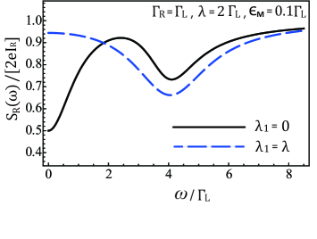
Figure 12: Shot noise which reveals a spectral dip and zero-frequency enhancement effect. The former behavior reflects existence of coherent oscillations which indicates the formation of a bound state coupled to the quantum dot, and the latter originates from the nature of Majorana excitation. “$\lambda_{1}=\lambda$” corresponds to the Majorana bound state and “$\lambda_{1}=0$” to a regular one. As in Fig. 11, we set $\epsilon_{D}=0$ in this plot.

Figure 12 displays the representative result for the shot noise spectrum. First, we notice that a spectral dip appears at the frequency $\omega_{c}\simeq 2\lambda$ (for $\epsilon_{D}=0$ and small $\epsilon_{M}$), which reflects an existence of coherent oscillations in the central system, where is $\omega_{c}$ the characteristic frequency. This is an important signature, since it indicates the emergence of bound states at the ends of the wire with discrete energy, gapped from other higher energy continuum. Here, we should note that the quantum dot is coupled to a nanowire, and hence, in the usual case, the wire states are extended and have continuous energies, which cannot support coherent oscillations as indicated by the spectral “dip” in Fig. 12. As a comparison, in Fig. 12, we also plot the result of the same quantum dot coupling to a regular bound state with the same strength ($\lambda$). While an “oscillation dip” appears similarly at the same frequency, nevertheless, the zero (and low) frequency noise differs remarkably from the Majorana case.

To characterize the zero frequency noise, we use the well-known Fano Factor, $F_{\alpha}=S_{\alpha}(0)/2eI_{\alpha}^{s}$. For symmetric rates $\Gamma_{R}=\Gamma_{L}=\Gamma_{0}$, we find $F_{L}=F_{R}$ and denote the Fano factor simply by $F$. Analytically, we obtain MF-1

$$F-F^{\rm(R)}\!=\frac{2\lambda^{2}\lambda_{1}^{2}}{(\Gamma_{0}^{2}+\epsilon_{M}^{2})(\lambda^{2}+\lambda_{1}^{2})+4\lambda^{2}\lambda_{1}^{2}}.$$ (58)

Here, $F^{\rm(R)}$ is the Fano factor of coupling to a regular (R) bound state. Moreover, in this result, we distinguish the coupling amplitudes $\lambda$ and $\lambda_{1}$ (introduced in the coupling Hamiltonian). We notice that $\lambda$ and $\lambda_{1}$ play identical (symmetric) roles and the difference, Eq. (58), vanishes if any of the amplitudes disappears. We then understand that the zero-frequency noise enhancement is arising from the peculiar nature of the Majorana excitation. Therefore, the noise enhancement effect in Fig. 12 is another useful signature for Majorana excitation at the ends of the nanowire. In addition, Eq. (58) can be used to obtain the important parameters of the Majorana’s mutual interaction ($\epsilon_{M}$) and its coupling to the quantum dot ($\lambda$). In particular, based on Eq. (58), after setting $\lambda_{1}=\lambda$ for the Majorana fermion, an even simpler result can be obtained in the limit $\epsilon_{M}\rightarrow 0$ i.e., $F=1-\frac{1}{2}[1+2(\lambda/\Gamma_{0})^{2}]^{-1}$. This result provides a very simple relation between the Fano factor and the scaled coupling amplitude ($\lambda/\Gamma_{0}$).

Now, we consider $\Gamma_{L}\neq\Gamma_{R}$. Taking the limit $\epsilon_{M}\rightarrow 0$ and setting $\epsilon_{D}=0$, we obtain MF-1

$$F_{R}=\frac{\Gamma_{L}^{2}+\Gamma_{R}^{2}}{\Gamma^{2}}+\frac{8\Gamma_{R}\Gamma_{L}\lambda^{2}\left[(5-3y)\Gamma^{2}+16\lambda^{2}\right]}{\Gamma^{2}(\Gamma^{2}+8\lambda^{2})^{2}},$$ (59a)

$$F_{L}=\frac{\Gamma_{L}^{2}+\Gamma_{R}^{2}}{\Gamma^{2}}+\frac{8\Gamma_{R}\Gamma_{L}\lambda^{2}\left[(5-3/y)\Gamma^{2}+16\lambda^{2}\right]}{\Gamma^{2}(\Gamma^{2}+8\lambda^{2})^{2}},$$ (59b)

We notice that the first term in $F_{L(R)}$ is the Fano factor corresponding to transport through an isolated single-level quantum dot Li053 ; ChT91 , while the second term arises from coupling to the Majorana fermion. If $\Gamma_{L}\neq\Gamma_{R}$, we find that $F_{R}-F_{L}=24(\Gamma_{L}-\Gamma_{R})\Gamma\lambda^{2}/(\Gamma^{2}+8\lambda^{2})^{2}\neq 0$. (This difference vanishes when $\Gamma_{L}=\Gamma_{R}$.) Finally, we mention that the steady-state current through the quantum dot cannot reveal the Majorana information in the symmetric case ($\Gamma_{L}=\Gamma_{R}$) MF-1 . However, the Fano factor given above carries such information, since the second term in $F_{L(R)}$ does not vanish when $y=1$. Note also that, if the quantum dot couples to a regular bound state (another dot), the zero frequency noise (Fano factor) is the same as the first term of the above $F_{L(R)}$, being unaffected by the side coupling.

V Master Equation under Self-consistent Born Approximation

In this section,

we review our recent work on improving the ME beyond the second-order Born approximation SCBA-1 ; SCBA-2 ; SCBA-3 . The basic idea is to base the formulation on the self-consistent Born approximation. That is, we replace the free Green’s function in the tunneling self-energy diagram by an effective reduced propagator under the Born approximation SCBA-1 . Remarkably, we will see that this modification can greatly improve the results.

In some cases (such as in quantum optics), the second-order ME works perfectly well. However, for quantum transport, the second-order expansion of the tunneling Hamiltonian only corresponds to sequential transport, which does not incorporate the level broadening effect Li05b , implying thus a validity condition of large bias voltage. Moreover, for interacting systems, although the second-order ME can predict the Coulomb staircase behavior, it cannot deal with the cotunneling and Kondo effects. To overcome this limitation, higher-order expansions of the tunneling Hamiltonian are required Sch94 ; Sch96 ; Sch06 ; Yan080911 ; Yan2012 ; Wac05+10 ; CS11 ; Leeu09 ; Galp09 ; Galp10 ; KG13 .

The second-order ME is obtained from the well-known Born approximation through perturbative expansion of the tunneling Hamiltonian Li05b . The resultant dissipation term, in analogy to the quantum dissipative system, corresponds to a self-energy process of tunneling. On the other hand, it is well known that in the Green’s function theory, an efficient scheme of higher-order correction is the use of renormalized self-energy diagram under the self-consistent Born approximation (SCBA), which is actually a type of self-consistent renormalization to the bare propagator with a dressed one Mat . From this insight, for quantum transport we may replace the free (system-Hamiltonian only) Green’s function in the second-order self-energy diagram, with an effective propagator defined by the second-order ME SCBA-1 . We will see that the effect of this improvement is remarkable: it recovers not only the exact result of noninteracting transport under arbitrary voltages but also the cotunneling and nonequilibrium Kondo features for interacting systems.

V.1 Formulation of the SCBA-ME

V.1.1 Master equation under Born approximation

In a more compact form

, we reexpress the ME (11) (under the second-order Born approximation) as SCBA-1 ; SCBA-2 ; SCBA-3

$$\dot{\rho}(t) =-i{\cal L}\rho(t)-\sum_{\mu\sigma}\Big{\{}\big{[}a^{\bar{\sigma}}_{\mu},A^{(\sigma)}_{\mu\rho}(t)\big{]}+{\rm H.c.}\Big{\}}.$$ (60)

Here, we introduced: $\sigma=+$ and $-$, $\bar{\sigma}=-\sigma$; $a^{+}_{\mu}=a^{\dagger}_{\mu}$, and $a^{-}_{\mu}=a_{\mu}$. The superoperators can be expressed as ${\cal L}\rho=[H_{S},\rho]$, and $A^{(\sigma)}_{\mu\rho}(t)=\sum_{\alpha=L,R}A^{(\sigma)}_{\alpha\mu\rho}(t)$ while $A^{(\sigma)}_{\alpha\mu\rho}(t)=\sum_{\nu}\int^{t}_{0}d\tau C^{(\sigma)}_{\alpha\mu\nu}(t-\tau)\left\{{\cal G}(t,\tau)[a^{\sigma}_{\nu}\rho(\tau)]\right\}$. ${\cal G}(t,\tau)$ is the free propagator, determined by the system Hamiltonian as ${\cal G}(t,\tau)=e^{-i{\cal L}(t-\tau)}$.

Now we present a specific characterization for $C^{(\sigma)}_{\alpha\mu\nu}(t-\tau)$ in terms of its Fourier transform:

$$C^{(\pm)}_{\alpha\mu\nu}(t-\tau)=\int^{\infty}_{-\infty}\frac{d\omega}{2\pi}e^{\pm i\omega(t-\tau)}\Gamma^{(\pm)}_{\alpha\mu\nu}(\omega).$$ (61)

Accordingly, we have $\Gamma^{(+)}_{\alpha\mu\nu}(\omega)=\Gamma_{\alpha\nu\mu}(\omega)n^{(+)}_{\alpha}(\omega)$ and $\Gamma^{(-)}_{\alpha\mu\nu}(\omega)=\Gamma_{\alpha\mu\nu}(\omega)n^{(-)}_{\alpha}(\omega)$, where $\Gamma_{\alpha\mu\nu}(\omega)=2\pi\sum_{k}t_{\alpha\mu k}t^{\ast}_{\alpha\nu k}\delta(\omega-\epsilon_{k})$ is the spectral density function of the reservoir ($\alpha$), $n^{(+)}_{\alpha}(\omega)$ denotes the Fermi function $n_{\alpha}(\omega)$, and $n^{(-)}_{\alpha}(\omega)=1-n_{\alpha}(\omega)$ is introduced for brevity. Alternatively, we may introduce the Laplace transform of $C^{(\sigma)}_{\alpha\mu\nu}(t-\tau)$, denoted by $C^{(\sigma)}_{\alpha\mu\nu}(\omega)$, which is related to $\Gamma^{(\pm)}_{\alpha\mu\nu}(\omega)$ through the well known dispersive relation:

$$C^{(\pm)}_{\alpha\mu\nu}(\omega) =\int^{\infty}_{-\infty}\frac{d\omega^{\prime}}{2\pi}\frac{i}{\omega\pm\omega^{\prime}+i0^{+}}\Gamma^{(\pm)}_{\alpha\mu\nu}(\omega^{\prime}).$$ (62)

For the reservoir spectral density function, we assume a Lorentzian form as

$$\Gamma_{\alpha\mu\nu}(\omega)=\frac{\Gamma_{\alpha\mu\nu}W^{2}_{\alpha}}{(\omega-\mu_{\alpha})^{2}+W^{2}_{\alpha}}.$$ (63)

Here, we use the constant $\Gamma_{\alpha\mu\nu}$ (without the argument $\omega$) to denote the height of the Lorentzian spectrum, and $W_{\alpha}$ to characterize its bandwidth. The form of Eq. (63) also corresponds to a half-occupied band for each lead, which peaks the Lorentzian center at the chemical potential $\mu_{\alpha}$ of the lead. Obviously, the usual constant spectral density function is obtained from Eq. (63) in the limit $W_{\alpha}\rightarrow\infty$, yielding $\Gamma_{\alpha\mu\nu}(\omega)=\Gamma_{\alpha\mu\nu}$. Corresponding to the Lorentzian spectral density function, straightforwardly, we obtain

$$C^{(\pm)}_{\alpha\mu\nu}(\omega) =\frac{1}{2}\left[\Gamma^{(\pm)}_{\alpha\mu\nu}(\mp\omega)+i\Lambda^{(\pm)}_{\alpha\mu\nu}(\mp\omega)\right].$$ (64)

The imaginary part, through the dispersive relation, is associated with the real part as

$$\Lambda^{(\pm)}_{\alpha\mu\nu}(\omega)={\cal P}\int^{\infty}_{-\infty}\frac{d\omega^{\prime}}{2\pi}\frac{1}{\omega\pm\omega^{\prime}}\Gamma^{(\pm)}_{\alpha\mu\nu}(\omega)$$

$$=\frac{\Gamma_{\alpha\mu\nu}}{\pi}\Bigg{\{}{\rm Re}\left[\Psi\left(\frac{1}{2}+i\frac{\beta(\omega-\mu_{\alpha})}{2\pi}\right)\right]$$

$$\quad-\Psi\left(\frac{1}{2}+\frac{\beta W_{\alpha}}{2\pi}\right)\mp\pi\frac{\omega-\mu_{\alpha}}{W_{\alpha}}\Bigg{\}},$$ (65)

where ${\cal P}$ represents the principle value, $\Psi(x)$ is the digamma function, and $\beta=1/k_{B}T$ denotes the inverse temperature.

The second-order ME can be applied only to transport under large bias voltage i.e., the Fermi levels of the leads should be considerably away from the system levels, by at least several times of the level’s broadening.

V.1.2 Master equation under self-consistent Born approximation

The basic idea

to improve the second-order ME can follow what is typically done in the Green’s function theory, i.e., correcting the self-energy diagram from the Born to a self-consistent Born approximation. In our case, the SCBA scheme can be implemented by replacing the free propagator in the second-order ME, ${\cal G}(t,\tau)=e^{-i{\cal L}(t-\tau)}$, by an effective one, ${\cal U}(t,\tau)$, which propagates a state with the precision of the second-order Born approximation, given by Eq. (60). From this consideration, the generalized SCBA-ME follows Eq. (60) directly as SCBA-1

$$\dot{\rho}(t) =-i{\cal L}\rho(t)-\sum_{\mu\sigma}\Big{\{}\big{[}a^{\bar{\sigma}}_{\mu},{\cal A}^{(\sigma)}_{\mu\rho}(t)\big{]}+{\rm H.c.}\Big{\}}.$$ (66)

Here, ${\cal A}^{(\sigma)}_{\mu\rho}(t)=\sum_{\alpha=L,R}{\cal A}^{(\sigma)}_{\alpha\mu\rho}(t)$, and ${\cal A}^{(\sigma)}_{\alpha\mu\rho}(t)=\sum_{\nu}\int^{t}_{0}d\tau C^{(\sigma)}_{\alpha\mu\nu}(t-\tau)\left\{{\cal U}(t,\tau)[a^{\sigma}_{\nu}\rho(\tau)]\right\}$. To close this ME, let us define $\tilde{\rho}_{j}(t)\equiv{\cal U}(t,\tau)[a^{\sigma}_{\nu}\rho(\tau)]$ (here and in the following equation we use “$j$” to denote the double indices $(\nu,\sigma)$ for the sake of brevity). Then, the equation-of-motion (EOM) of this auxiliary object is given as SCBA-1

$$\dot{\tilde{\rho}}_{j}(t)=-i{\cal L}\tilde{\rho}_{j}(t)-\int^{t}_{\tau}dt^{\prime}\Sigma^{(A)}_{2}(t-t^{\prime})\tilde{\rho}_{j}(t^{\prime}).$$ (67)

In this equation, we introduce a notation $\Sigma^{(A)}_{2}$ for the second-order self-energy superoperator, where the superscript “$(A)$” indicates an essential difference from the usual one because it involves anticommutators, rather than the commutators in the second-order ME. More explicitly, we have SCBA-1

$$\int^{t}_{\tau}dt^{\prime}\Sigma^{(A)}_{2}(t-t^{\prime}) \tilde{\rho}_{j}(t^{\prime})=\sum_{\mu}\Big{[}\big{\{}a_{\mu},A^{(+)}_{\mu\tilde{\rho}_{j}}\big{\}}+\big{\{}a^{\dagger}_{\mu},A^{(-)}_{\mu\tilde{\rho}_{j}}\big{\}}$$

$$+\big{\{}a^{\dagger}_{\mu},A^{(+)\dagger}_{\mu\tilde{\rho}_{j}}\big{\}}+\big{\{}a_{\mu},A^{(-)\dagger}_{\mu\tilde{\rho}_{j}}\big{\}}\Big{]},$$ (68)

where $A^{(\pm)}_{\mu\tilde{\rho}_{j}}$ is defined as $A^{(\sigma^{\prime})}_{\mu\tilde{\rho}_{j}}=\sum_{\alpha=L,R}\sum_{\nu^{\prime}}\int^{t}_{\tau}dt^{\prime}C^{(\sigma^{\prime})}_{\alpha\mu\nu^{\prime}}(t-t^{\prime})\left\{e^{-i{\cal L}(t-t^{\prime})}[a^{\sigma^{\prime}}_{\nu^{\prime}}\tilde{\rho}_{j}(t^{\prime})]\right\}$. Because of the anticommutative brackets that appearing in Eq. (V.1.2), we stress that the propagation of $\tilde{\rho}_{j}(t)$ is not governed by the usual second-order ME. This, in certain sense, violates the celebrated quantum regression theorem. We notice that the second-order reduced propagator ${\cal U}$ was introduced from $\rho(t)={\cal U}(t,t_{0})\rho(t_{0})$, and in Eq. (67), the quantity being propagated is $a^{\sigma}_{\nu}\rho(t_{0})$, which differs from the former only by an initial condition. Then, from experience, we may expect that the propagator must be independent of the initial condition, in the present context, which is the object to be propagated. In most cases, this statement is true. However, our analysis shows that this general rule (the celebrated quantum regression theorem), quite unexpectedly, is not followed in the present case. The basic reason is that the object being propagated, $a^{\sigma}_{\nu}\rho$, contains an extra electron operator. Owing to the Pauli principle (or Fermi-Dirac statistics), extra negative signs appear in two of the four self-energy terms in its equation-of-motion. This changes the commutators in the usual master equation to the anti-commutators in Eq. (V.1.2). We find that this subtle issue is extremely important – otherwise we cannot obtain the correct results such as the illustrative examples in this work.

V.1.3 Steady state current

Within the framework of SCBA-ME

, similar to its second-order counterpart, the current through the $\alpha$th lead is given as SCBA-1

$$I_{\alpha}(t)=2\sum_{\mu}{\rm Re}\left\{{\rm Tr}\big{[}{\cal A}^{(+)}_{\alpha\mu\rho}(t)a_{\mu}-{\cal A}^{(-)}_{\alpha\mu\rho}(t)a^{\dagger}_{\mu}\big{]}\right\}.$$ (69)

Here, ${\rm Re}\{\cdots\}$ indicates the real part of $\{\cdots\}$ and ${\rm Tr}[\cdots]$ is the trace of $[\cdots]$ over the system only states. For steady state, consider the integral $\int^{t}_{0}d\tau[\cdots]\rho(\tau)$ in ${\cal A}^{(\pm)}_{\alpha\mu\rho}(t)$. Since physically, the correlation function $C^{(\pm)}_{\alpha\mu\nu}(t-\tau)$ in the integrand is nonzero only on finite timescale, we can replace $\rho(\tau)$ in the integrand by the steady state $\bar{\rho}$, in the long time limit ($t\rightarrow\infty$). After this replacement, we obtain

$${\cal A}^{(\pm)}_{\alpha\mu\bar{\rho}}=\sum_{\nu}\int^{\infty}_{-\infty}\frac{d\omega}{2\pi}\,\Gamma^{(\pm)}_{\alpha\mu\nu}(\omega){\cal U}(\pm\omega)[a^{\pm}_{\nu}\bar{\rho}].$$ (70)

Then, substituting this result into Eq. (66), we can directly solve for $\bar{\rho}$, and calculate the steady state current.

Based on $\bar{\rho}$, in order to further obtain the current, we first introduce $\varphi_{1\mu\nu}(\omega)={\rm Tr}\big{[}a_{\mu}\tilde{\rho}_{1\nu}(\omega)\big{]}$ and $\varphi_{2\mu\nu}(\omega)={\rm Tr}\big{[}a_{\mu}\tilde{\rho}_{2\nu}(\omega)\big{]}$, where $\tilde{\rho}_{1\nu}(\omega)$ and $\tilde{\rho}_{2\nu}(\omega)$ are calculated using Eq. (67), with an initial condition of $\tilde{\rho}_{1\nu}(0)=\bar{\rho}a^{\dagger}_{\nu}$ and $\tilde{\rho}_{2\nu}(0)=a^{\dagger}_{\nu}\bar{\rho}$. To simplify the notations, we denote the various matrices expanded in the system state basis $\{|\mu\rangle,|\nu\rangle\}$ in terms of a boldface form: $\bm{\varphi}_{1}(\omega)$, $\bm{\varphi}_{2}(\omega)$, and $\bm{\Gamma}_{L(R)}$. If $\bm{\Gamma}_{L}$ is proportional to $\bm{\Gamma}_{R}$ by a constant, the steady state current can be recast to the Landauer-Büttiker type SCBA-1

$$\bar{I}=2~{}{\rm Re}\int^{\infty}_{-\infty}\frac{d\omega}{2\pi}\left[n_{L}(\omega)-n_{R}(\omega)\right]{\cal T}(\omega),$$ (71)

where the tunneling coefficient, very compactly, is given by

$${\cal T}(\omega)={\rm Tr}\{\bm{\Gamma}_{L}\bm{\Gamma}_{R}(\bm{\Gamma}_{L}+\bm{\Gamma}_{R})^{-1}{\rm Re}\big{[}\bm{\varphi}(\omega)\big{]}\}.$$ (72)

Here, $\bm{\varphi}(\omega)=\bm{\varphi}_{1}(\omega)+\bm{\varphi}_{2}(\omega)$.

Now, we demonstrate that for a noninteracting system, the above stationary current coincides precisely with the nonequilibrium Green’s function approach, both giving the exact result under a arbitrary bias voltage. In general, a noninteracting system can be described by $H_{S}=\sum_{\mu\nu}h_{\mu\nu}a^{\dagger}_{\mu}a_{\nu}$. We directly obtain the EOM of $\bm{\varphi}_{i}$ as follows:

$$-i\omega\bm{\varphi}_{i}(\omega)-\bm{\varphi}_{i}(0)=-i\bm{h}\bm{\varphi}_{i}(\omega)-i\bm{\Sigma}_{0}(\omega)\bm{\varphi}_{i}(\omega).$$ (73)

$\bm{\varphi}_{i}(0)$ denotes the initial conditions for $\varphi_{1\mu\nu}(0)={\rm Tr}\big{[}a_{\mu}\bar{\rho}a^{\dagger}_{\nu}\big{]}$ and $\varphi_{2\mu\nu}(0)={\rm Tr}\big{[}a_{\mu}a^{\dagger}_{\nu}\bar{\rho}\big{]}$. The tunnel-coupling self-energy $\bm{\Sigma}_{0}$ is given by $\Sigma_{0\mu\nu}(\omega)=-i\sum_{\alpha}\big{[}C^{(-)}_{\alpha\mu\nu}(\omega)+C^{(+)\ast}_{\alpha\mu\nu}(-\omega)\big{]}$, or

$$\Sigma_{0\mu\nu}(\omega) =\int^{\infty}_{-\infty}\frac{d\omega^{\prime}}{2\pi}\frac{\Gamma_{\mu\nu}(\omega^{\prime})}{\omega-\omega^{\prime}+i0^{+}}.$$ (74)

Then, based on Eq. (73), summing up $\bm{\varphi}_{1}(\omega)$ and $\bm{\varphi}_{2}(\omega)$ we obtain

$$\bm{\varphi}(\omega)=i\big{[}\omega-\bm{h}-\bm{\Sigma}_{0}(\omega)\big{]}^{-1}$$ (75)

For deriving this result, the cyclic property under trace and the anti-commutator, $\{a_{\mu},a^{\dagger}_{\nu}\}=\delta_{\mu\nu}$, have been used. Eq. (75) is nothing but the exact Green’s function for transport through a noninteracting system, thus giving the exact stationary current after inserting it into the above current formula.

V.1.4 Interacting case

To show the application of the proposed SCBA-ME

in interacting systems, as an illustrative example, we consider the transport through an interacting quantum dot described as:

$$H_{S}=\sum_{\mu}\left(\epsilon_{\mu}a_{\mu}^{\dagger}a_{\mu}+\frac{U}{2}n_{\mu}n_{\bar{\mu}}\right).$$ (76)

Here, the index $\mu$ labels the spin up (“$\uparrow$”) and spin down (“$\downarrow$”) states, and $\bar{\mu}$ represents the opposite spin orientation. $\epsilon_{\mu}$ denotes the spin-dependent energy level, which may account for the Zeeman splitting in the presence of a magnetic field ($B$), $\epsilon_{\uparrow,\downarrow}=\epsilon_{0}\pm g\mu_{B}B$. Here, $\epsilon_{0}$ is the degenerate dot level in the absence of a magnetic field; $g$ and $\mu_{B}$ are the Lande-$g$ factor and the Bohr’s magneton, respectively. In the interaction part, $Un_{\uparrow}n_{\downarrow}$ is the Hubbard term, $n_{\mu}=a^{\dagger}_{\mu}a_{\mu}$ is the number operator, and $U$ represents the interacting strength.

First, we notice that $C^{(\pm)}_{\alpha\mu\nu}$ is diagonal with respect to the spin states, i.e., $C^{(\pm)}_{\alpha\mu\nu}(t)=\delta_{\mu\nu}C^{(\pm)}_{\alpha\mu}(t)$ and $\Gamma^{(\pm)}_{\alpha\mu\nu}=\delta_{\mu\nu}\Gamma^{(\pm)}_{\alpha\mu}$. Here, $\delta_{\mu\nu}$ is the usual $\delta$-function with discrete indices, and in $C^{(\pm)}_{\alpha\mu}$ and $\Gamma^{(\pm)}_{\alpha\mu}$, there is only a single state index ($\mu$) for brevity. Then, we specify the states involved in the transport as $|0\rangle$, $|\uparrow\rangle$, $|\downarrow\rangle$, and $|d\rangle$, corresponding to the empty, spin-up, spin-down, and double occupancy states, respectively, Using this basis, we reexpress the electron operator in terms of projection operator, $a^{\dagger}_{\mu}=|\mu\rangle\langle 0|+(-1)^{\mu}|d\rangle\langle\bar{\mu}|$, where the conventions $(-1)^{\uparrow}=1$ and $(-1)^{\downarrow}=-1$ are implied. For a solution of the steady state, we have SCBA-1

$${\cal A}^{(\pm)}_{\alpha\mu\bar{\rho}} =\int^{\infty}_{-\infty}\frac{d\omega}{2\pi}\,\Gamma^{(\pm)}_{\alpha\mu}(\omega){\cal U}(\pm\omega)[a^{\pm}_{\mu}\bar{\rho}].$$ (77)

Thus, after some calculations, ${\cal U}(\pm\omega)[a^{\pm}_{\mu}\bar{\rho}]$ can be expressed as

$${\cal U}(\omega)[a^{\dagger}_{\mu}\bar{\rho}] =\left[\lambda^{+}_{\mu}(\omega)|\mu\rangle\langle 0|+\kappa^{+}_{\mu}(\omega)(-1)^{\mu}|d\rangle\langle\bar{\mu}|\right],$$

$${\cal U}(-\omega)[a_{\mu}\bar{\rho}] =\left[\lambda^{-}_{\mu}(\omega)|0\rangle\langle\mu|+\kappa^{-}_{\mu}(\omega)(-1)^{\mu}|\bar{\mu}\rangle\langle d|\right],$$ (78)

where

$$\lambda^{+}_{\mu}(\omega) =i\frac{\Pi^{-1}_{1\mu}(\omega)\bar{\rho}_{00}-\Sigma^{-}_{\bar{\mu}}(\omega)\bar{\rho}_{\bar{\mu}\bar{\mu}}}{\Pi^{-1}_{\mu}(\omega)\Pi^{-1}_{1\mu}(\omega)},$$

$$\lambda^{-}_{\mu}(\omega) =i\frac{\Pi^{-1}_{1\mu}(\omega)\bar{\rho}_{\mu\mu}-\Sigma^{-}_{\bar{\mu}}(\omega)\bar{\rho}_{dd}}{\Pi^{-1}_{\mu}(\omega)\Pi^{-1}_{1\mu}(\omega)},$$

$$\kappa^{+}_{\mu}(\omega) =i\frac{-\Sigma^{+}_{\bar{\mu}}(\omega)\bar{\rho}_{00}+\Pi^{-1}_{\mu}(\omega)\bar{\rho}_{\bar{\mu}\bar{\mu}}}{\Pi^{-1}_{\mu}(\omega)\Pi^{-1}_{1\mu}(\omega)},$$

$$\kappa^{-}_{\mu}(\omega) =i\frac{-\Sigma^{+}_{\bar{\mu}}(\omega)\bar{\rho}_{\mu\mu}+\Pi^{-1}_{\mu}(\omega)\bar{\rho}_{dd}}{\Pi^{-1}_{\mu}(\omega)\Pi^{-1}_{1\mu}(\omega)}.$$

Here, we introduced $\Pi^{-1}_{\mu}(\omega)=\omega-\epsilon_{\mu}-\Sigma_{0\mu}(\omega)-\Sigma^{+}_{\bar{\mu}}(\omega)$, and $\Pi^{-1}_{1\mu}(\omega)=\omega-\epsilon_{\mu}-U-\Sigma_{0\mu}(\omega)-\Sigma^{-}_{\bar{\mu}}(\omega)$. The self-energies $\Sigma_{0\mu}(\omega)$ and $\Sigma^{\pm}_{\mu}(\omega)$ are given by

$$\Sigma_{0\mu}(\omega) =\int^{\infty}_{-\infty}\frac{d\omega^{\prime}}{2\pi}\frac{\Gamma_{\mu}(\omega^{\prime})}{\omega-\omega^{\prime}+i0^{+}},$$

$$\Sigma^{\pm}_{\mu}(\omega) =\int^{\infty}_{-\infty}\frac{d\omega^{\prime}}{2\pi}\frac{\Gamma^{(\pm)}_{\mu}(\omega^{\prime})}{\omega-\epsilon_{\bar{\mu}}+\epsilon_{\mu}-\omega^{\prime}+i0^{+}}$$

$$+\int^{\infty}_{-\infty}\frac{d\omega^{\prime}}{2\pi}\frac{\Gamma^{(\pm)}_{\mu}(\omega^{\prime})}{\omega-E_{d}+\omega^{\prime}+i0^{+}}.$$ (79)

Then, we find the solution of $\bm{\varphi}(\omega)$ as

$$\bm{\varphi}(\omega)=\frac{i(1-n_{\bar{\mu}})}{\omega-\epsilon_{\mu}-\Sigma_{0\mu}+U\Sigma^{+}_{\bar{\mu}}(\omega-\epsilon_{\mu}-U-\Sigma_{0\mu}-\Sigma_{\bar{\mu}})^{-1}}$$

$$~{}+\frac{in_{\bar{\mu}}}{\omega-\epsilon_{\mu}-U-\Sigma_{0\mu}-U\Sigma^{-}_{\bar{\mu}}(\omega-\epsilon_{\mu}-\Sigma_{0\mu}-\Sigma_{\bar{\mu}})^{-1}},$$ (80)

where $n_{\mu}=\rho_{\mu\mu}+\rho_{dd}$, and $1-n_{\mu}=\rho_{\bar{\mu}\bar{\mu}}+\rho_{00}$. This result coincides precisely with the one from the EOM technique of the nonequilibrium Green’s function Jau96 , which contains the remarkable nonequilibrium Kondo effect.

At high temperatures, Eq. (V.1.4) reduces to

$$\bm{\varphi}_{HF}(\omega)=\frac{i(1-n_{\bar{\mu}})}{\omega-\epsilon_{\mu}-\Sigma_{0\mu}}+\frac{in_{\bar{\mu}}}{\omega-\epsilon_{\mu}-U-\Sigma_{0\mu}}.$$ (81)

Here, we use $\bm{\varphi}_{HF}$ to indicate the result at the level of a mean-field Hatree-Fock approximation. Eq. (81) can also be derived from the EOM technique at a lower-order cutoff Jau96 . As a result, even the simple broadening effect contained in Eq. (81) goes beyond the scope of the second-order ME. In Fig. 13, we plot the current-voltage relation based on Eq. (V.1.4) against that from Eq. (81).

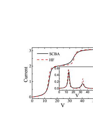
Figure 13: Coulomb staircase in the current-voltage curve. Inset: the corresponding differential conductance. The result based on Eq. (V.1.4) is plotted against the Hatree-Fock (HF) solution Eq. (81). Parameters: $\Gamma_{L}=\Gamma_{R}=\Gamma/2$, $\epsilon_{0}=7\Gamma$, $U=10\Gamma$, and $k_{B}T=0.1\Gamma$. The bias voltage is set as $\mu_{L}=-\mu_{R}=eV/2$ by taking the zero-bias Fermi level as energy reference.

V.2 Formulation of the $n$-SCBA-ME

Let us turn to the construction of the $n$-resolved SCBA-ME ($n$-SCBA-ME), along the same line of constructing the $n$-resolved second-order ME SCBA-2 ; SCBA-3 . The basic idea is to split the Hilbert space of the reservoirs into a set of subspaces, each labeled by $n$. Then, the average (trace) over each subspace is calculated, and the corresponding conditional reduced density matrix is defined as $\rho^{(n)}(t)$. To be specific, consider the $\rho^{(n)}(t)$ conditioned on the electron number arrived to the right lead, which obeys the following equation SCBA-2 ; SCBA-3

$$\dot{\rho}^{(n)} =-i{\cal L}\rho^{(n)}-\sum_{\mu}\Big{\{}\big{[}a_{\mu}^{\dagger}{\cal A}_{\mu\tilde{\rho}^{(n)}}^{(-)}+a_{\mu}{\cal A}_{\mu\tilde{\rho}^{(n)}}^{(+)}-{\cal A}_{L\mu\tilde{\rho}^{(n)}}^{(-)}a_{\mu}^{\dagger}$$

$$-{\cal A}_{L\mu\tilde{\rho}^{(n)}}^{(+)}a_{\mu}-{\cal A}_{R\mu\tilde{\rho}^{(n-1)}}^{(-)}a_{\mu}^{\dagger}-{\cal A}_{R\mu\tilde{\rho}^{(n+1)}}^{(+)}a_{\mu}\big{]}+{\rm H.c.}\Big{\}}.$$ (82)

Here, ${\cal A}^{(\sigma)}_{\alpha\mu\tilde{\rho}^{(n)}}(t)=\sum_{\nu}\int^{t}_{0}d\tau C^{(\sigma)}_{\alpha\mu\nu}(t-\tau)[\tilde{\rho}_{j}^{(n)}(t,\tau)]$, while the summation over $\nu$ is appropriate in regard to the abbreviation $j=\{\nu,\sigma\}$. In Eq. (V.2), the appearance of $\tilde{\rho}^{(n\pm 1)}_{j}(t,\tau)$ is owing to a more tunneling event (forward/backword) involved in the process of the corresponding terms. In particular, $\tilde{\rho}_{j}^{(n)}(t,\tau)$ is the $n$-dependent version of the quantity $\tilde{\rho}_{j}(t,\tau)={\cal U}(t,\tau)[a^{\sigma}_{\nu}\rho(\tau)]$, satisfying the EOM according to Eq. (67):

$$\dot{\tilde{\rho}}^{(n)}_{j} =-i{\cal L}\tilde{\rho}^{(n)}_{j}-\sum_{\mu}\Big{\{}\big{[}a_{\mu}^{\dagger}A_{\mu\tilde{\rho}^{(n)}_{j}}^{(-)}+a_{\mu}A_{\mu\tilde{\rho}^{(n)}_{j}}^{(+)}+A_{L\mu\tilde{\rho}^{(n)}_{j}}^{(-)}a_{\mu}^{\dagger}$$

$$+A_{L\mu\tilde{\rho}^{(n)}_{j}}^{(+)}a_{\mu}+A_{R\mu\tilde{\rho}^{(n-1)}_{j}}^{(-)}a_{\mu}^{\dagger}+A_{R\mu\tilde{\rho}^{(n+1)}_{j}}^{(+)}a_{\mu}\big{]}+{\rm H.c.}\Big{\}}.$$ (83)

In this equation, we introduced $A^{(\sigma^{\prime})}_{\alpha\mu\tilde{\rho}^{(n)}_{j}}(t)=\sum_{\nu^{\prime}}\int^{t}_{\tau}dt^{\prime}C^{(\sigma^{\prime})}_{\alpha\mu\nu^{\prime}}(t-t^{\prime})\left\{e^{-i{\cal L}(t-t^{\prime})}[a^{\sigma^{\prime}}_{\nu^{\prime}}\tilde{\rho}_{j}^{(n)}(t^{\prime})]\right\}$.

The $n$-resolved ME contains important information and can be used in a wide variety of applications. Next, we focus on calculating the shot noise spectrum $S(\omega)$, using the MacDonald’s formula $S(\omega)=2\omega\int^{\infty}_{0}dt\sin(\omega t)\frac{d}{dt}\langle n^{2}(t)\rangle$, where $\langle n^{2}(t)\rangle=\sum_{n}n^{2}P(n,t)={\rm Tr}\sum_{n}n^{2}\rho^{(n)}(t)$, and the $n$-counting starts with the steady state ($\bar{\rho}$). Based on Eq. (V.2), one can express $\frac{d}{dt}\langle n^{2}(t)\rangle$ in terms of ${\cal A}^{(\sigma)}_{R\mu\bar{\rho}}(t)$ and ${\cal A}^{(\sigma)}_{R\mu\tilde{N}}(t)$. The former has been introduced in Eq. (66), needing only to replace $\rho(\tau)$ by $\bar{\rho}$. The latter reads ${\cal A}^{(\sigma)}_{R\mu\tilde{N}}(t)=\sum_{\nu}\int^{t}_{0}d\tau C^{(\sigma)}_{R\mu\nu}(t-\tau)[\tilde{N}_{j}(t,\tau)]$, where $\tilde{N}_{j}(t,\tau)=\sum_{n}n\tilde{\rho}_{j}^{(n)}(t,\tau)$, noting also the abbreviation $j=\{\nu,\sigma\}$ which makes the summation over $\nu$ reasonable. Then, the MacDonald’s formula becomes:

$$S(\omega) =2\omega{\rm Im}\sum_{\mu}{\rm Tr}\Big{\{}2\big{[}{\cal A}_{R\mu\tilde{N}}^{(-)}(\omega)a_{\mu}^{\dagger}-{\cal A}_{R\mu\tilde{N}}^{(+)}(\omega)a_{\mu}\big{]}$$

$$\qquad\qquad+\big{[}{\cal A}_{R\mu\bar{\rho}}^{(-)}(\omega)a_{\mu}^{\dagger}+{\cal A}_{R\mu\bar{\rho}}^{(+)}(\omega)a_{\mu}\big{]}\Big{\}}.$$ (84)

This result is obtained after Laplace transforming ${\cal A}^{(\sigma)}_{R\mu\bar{\rho}}(t)$ and ${\cal A}^{(\sigma)}_{R\mu\tilde{N}}(t)$. More explicitly,

$${\cal A}^{(\sigma)}_{R\mu\bar{\rho}}(\omega)=\sum_{\nu}\int^{\infty}_{-\infty}\frac{d\omega^{\prime}}{2\pi}\Gamma^{(\sigma)}_{R\mu\nu}(\omega^{\prime}){\cal U}(\omega+\sigma\omega^{\prime})[a^{\sigma}_{\nu}\bar{\rho}(\omega)],$$

where the Laplace transformation of the steady state is given as $\bar{\rho}(\omega)=i\bar{\rho}/\omega$, and the propagator ${\cal U}$ in frequency domain is defined through Eq. (67). Another quantity, ${\cal A}^{(\sigma)}_{R\mu\tilde{N}}(\omega)$ is given as

$${\cal A}^{(\sigma)}_{R\mu\tilde{N}}(\omega)=\sum_{\nu}\int^{\infty}_{-\infty}\frac{d\omega^{\prime}}{2\pi}\Gamma^{(\sigma)}_{R\mu\nu}(\omega^{\prime})\tilde{\cal U}(\omega+\sigma\omega^{\prime})[a^{\sigma}_{\nu}N(\omega)].$$

In deriving this result, we introduced an additional propagator through $\tilde{N}_{j}(t,\tau)=\tilde{\cal U}(t-\tau)\tilde{N}_{j}(\tau)$, where $\tilde{N}_{j}(\tau)=a^{\sigma}_{\nu}N(\tau)$ as the initial condition which is defined by $N(\tau)=\sum_{n}n\rho^{(n)}(\tau)$. $\tilde{\cal U}(\omega)$ and $N(\omega)$ can be obtained via Laplace transforming the following EOMs. (i) For $N(\omega)$, based on the $n$-SCBA-ME we obtain:

$$\dot{N}(t) =-i{\cal L}N(t)-\sum_{\mu\sigma}\Big{\{}\big{[}a^{\bar{\sigma}}_{\mu},{\cal A}^{(\sigma)}_{\mu N}(t)\big{]}+{\rm H.c.}\Big{\}}$$

$$~{}~{}+\sum_{\mu}\Big{\{}\big{[}{\cal A}_{R\mu\bar{\rho}}^{(-)}a_{\mu}^{\dagger}-{\cal A}_{R\mu\bar{\rho}}^{(+)}a_{\mu}\big{]}+{\rm H.c.}\Big{\}}.$$ (85)

(ii) For $\tilde{\cal U}(\omega)$, from Eq. (V.2) we have

$$\dot{\tilde{N}}_{j}(t)=-i{\cal L}\tilde{N}_{j}(t)-\int^{t}_{\tau}dt^{\prime}{\Sigma}^{(A)}_{2}(t-t^{\prime})\tilde{N}_{j}(t^{\prime})$$

$$~{}-\sum_{\mu}\Big{\{}\big{[}A_{R\mu\tilde{\rho}_{j}}^{(-)}(t)a_{\mu}^{\dagger}-A_{R\mu\tilde{\rho}_{j}}^{(+)}(t)a_{\mu}\big{]}+{\rm H.c.}\Big{\}}.$$ (86)

The self-energy superoperator ${\Sigma}^{(A)}_{2}(t-t^{\prime})$ is referred to Eq. (V.1.2) for the definition and interepation/discussion. Similarly, as introduced in Eq. (V.2), we defined here $A^{(\sigma^{\prime})}_{R\mu\tilde{\rho}_{j}}(t)=\sum_{\nu^{\prime}}\int^{t}_{\tau}dt^{\prime}C^{(\sigma^{\prime})}_{R\mu\nu^{\prime}}(t-t^{\prime})\left\{e^{-i{\cal L}(t-t^{\prime})}[a^{\sigma^{\prime}}_{\nu^{\prime}}\tilde{\rho}_{j}(t^{\prime})]\right\}$.

For the convenience of applications, we summarize the solving procedures in a simpler way as follows. First, solve ${\cal U}(\omega)$ from Eq. (67) and obtain $\rho(\omega)$ from Eq. (66); then, extract $\tilde{\cal U}(\omega)$ from Eq. (V.2) and $N(\omega)$ from Eq. (V.2). Using $\tilde{\cal U}(\omega)$ and $N(\omega)$, we can directly calculate the noise spectrum of Eq. (V.2).

V.3 Noise Spectrum: Illustrative Examples

V.3.1 Noninteracting quantum dot

Let us first consider the simplest setup of transport through a single-level quantum dot. In the absence of the magnetic field and Coulomb interaction, the spin degree of freedom is irrelevant. Then, the system Hamiltonian is given as $H_{S}=\epsilon_{0}a^{\dagger}a$, and the states involved in the transport are $|0\rangle$ and $|1\rangle$, corresponding to the empty and occupied dot states. Applying the solving protocol outlined above, the shot noise spectrum can be directly obtained, as shown in Fig. 14 by the solid curve. As a comparison, in Fig. 14, we plot also the results from the second-order non-Markovian (nMKV) and Markovian (MKV) ME, respectively, by the dashed and dotted curves. The former is based on Ref. Jin2011 , while the later is from the following analytic result Li053

$$S(\omega)=2\bar{I}\left(\frac{\Gamma^{2}_{L}+\Gamma^{2}_{R}+\omega^{2}}{\Gamma^{2}+\omega^{2}}\right),$$ (87)

where $\Gamma=\Gamma_{L}+\Gamma_{R}$ is assumed. $\bar{I}$ is the steady state current, in large bias limit which is given as $\bar{I}=\Gamma_{L}\Gamma_{R}/\Gamma$, while here we account for the finite bias effect based on the SCBA-ME approach.

We observe that, quantitatively, the result from the $n$-SCBA-ME modifies that from the second-order nMKV-ME, while qualitatively both revealing a staircase behavior at frequency around $\omega_{\alpha 0}=|\mu_{\alpha}-\epsilon_{0}|$. Mathematically, the origin of the staircase is from the time-nonlocal memory effect. Physically, this behavior is owing to the detection-energy ($\omega$) assisted transmission resonance between the dot and leads, which experiences a sharp change when crossing the Fermi levels. In high frequency regime, the noise spectrum from the $n$-SCBA-ME coincides with that from the second-order nMKV-ME, while the latter is given in Ref. Jin2011 by the high frequency limit as $S(\omega\rightarrow\infty)=\Gamma_{R}$. This directly leads to a Fano factor as $F=S/2\bar{I}=(1+\Gamma_{R}/\Gamma_{L})/2$. Therefore, it can be Poissonian, sub-Poissonian, and super-Poissonian, depending on the symmetry factor $\Gamma_{R}/\Gamma_{L}$. In contrast, the second-order nMKV-ME predicts a Poissonian result, $F(\omega\rightarrow\infty)=1$.

We would like to point out that the second-order MKV-ME is only applicable in the low frequency regime of $\omega<\omega_{\alpha 0}=|\mu_{\alpha}-\epsilon_{0}|$. This is in consistency with the fact that the high frequency regime corresponds to a short timescale where the non-Markovian effect is strong, while the low frequency regime corresponds to a long timescale where the non-Markovian effect diminishes.

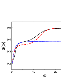
Figure 14: Shot noise spectrum through a single-level noninteracting quantum dot, from the SCBA-ME (solid curve), the 2nd-nMKV-ME (dashed curve) and the 2nd-MKV-ME (dotted curve), respectively. Parameters: $\Gamma_{L}=\Gamma_{R}=0.5$, $\mu_{L}=-\mu_{R}=7.5$, $\epsilon_{0}=5$, $k_{B}T=2$ and $W=100$.

V.3.2 Coulomb-Blockade quantum dot

This is the system described by Eq. (76). Here we first consider the noise spectrum in the Coulomb-Blockade (CB) regime, and leave the Kondo regime to next subsection. The CB regime of single occupation is characterized by $\epsilon_{0}+U>\mu_{L}>\epsilon_{0}>\mu_{R}$. For the purpose of comparison, we quote the result from the second-order MKV-ME Li053

$$S(\omega)=2\bar{I}\left[\frac{4\Gamma^{2}_{L}+\Gamma^{2}_{R}+\omega^{2}}{(2\Gamma_{L}+\Gamma_{R})^{2}+\omega^{2}}\right].$$ (88)

In large bias limit, i.e., the Fermi levels far from $\epsilon_{0}$ and $\epsilon_{0}+U$, the steady state current is given as $\bar{I}=2\Gamma_{L}\Gamma_{R}/(2\Gamma_{L}+\Gamma_{R})$. However, in numerical simulation, we account for the finite bias effect by inserting the steady state current from the SCBA-ME approach into Eq. (88). For obtaining Eq. (88), the double occupancy of the dot is excluded because the energy is out of the bias window. In the $n$-SCBA-ME treatment, however, all the four basis states should be included.

In Fig. 15, we display the main result of the noise spectrum in the CB regime, where a couple of non-Markovian resonance steps are revealed at frequencies around $\omega_{\alpha 0}=|\mu_{\alpha}-\epsilon_{0}|$ and $\omega_{\alpha 1}=\epsilon_{0}+U-\mu_{\alpha}$. We find that the resonance steps in high frequency regime are enhanced by the Coulomb interaction, while the low frequency spectrum has remarkable “renormalization” effect compared to Eq. (88). In addition to the result under the wide band limit (WBL), in Fig. 15, we also show the bandwidth effect by two more curves. We see that, for finite-bandwidth leads, the noise spectrum diminishes at the high frequency limit. This is because the energy ($\omega$) absorption/emission of detection restricts the channels for electron transfer between the dots and leads.

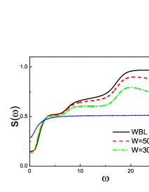
Figure 15: Shot noise spectrum through an interacting quantum dot in a Coulomb blockade regime defined as $\epsilon_{0}+U>\mu_{L}>\epsilon_{0}>\mu_{R}$. Results in the wide band limit (WBL) and for the finite bandwidths are shown in comparison with the one from the 2nd-MKV-ME (dotted line). Parameters: $\Gamma_{L}=\Gamma_{R}=0.5$, $\mu_{L}=-\mu_{R}=5$, $\epsilon_{\uparrow}=\epsilon_{\downarrow}=\epsilon_{0}=2$, $U=10$, and $k_{B}T=2$. We find staircases appearing at $\omega=\epsilon_{0}-\mu_{R}=7$ and $\epsilon_{0}+U-\mu_{R}=17$.

V.3.3 Nonequilibrium Kondo dot

The nonequilibroum Kondo system, with the Anderson impurity model realized by transport through a small quantum dot, has attracted intensive attentions Gor98 ; Kou98 ; Gla04 ; Ng88 ; Her91 ; MW92 ; MW9193 ; Ra94 ; Mar06 ; Gor08 ; Yan12 . Compared to the equilibrium Kondo effect, the nonequilibrium is characterized by a finite chemical potential difference of the two leads. As a result, the peak of the density of states (spectral function) splits into two peaks pinned at each chemical potential. The two peak structure is difficult to probe directly, by the usual dc measurements. Nevertheless, the shot noise might be a promising quantity to reveal the nonequilibrium Kondo effect, although much less is known about it. Despite the low-frequency noise measurements De09 ; Hei08 , so far there are no reports on the finite-frequency (FF) noise measurements. However, several theoretical studies Ng97 ; Her98 ; Kon07 ; Moc11 revealed diverse signatures (Kondo anomalies) in the FF noise spectra, such as an “upturn” Ng97 or a spectral “dip” Moc11 appeared at frequencies $\pm eV/\hbar$ ($V$ is the bias voltage), as well as the Kondo singularity (discontinuous slope) at frequencies $\pm 2eV/\hbar$ in Ref. Her98 , or at $\pm eV/2\hbar$ in Ref. Moc11 . In addition, it was noted in Ref. Her98 that the minimum (dip) developed at $\pm eV/\hbar$ is not relevant to the Kondo effect, since in the noninteracting case the noise has a similar discontinuous slope at $\pm eV/\hbar$ as well Her98 .

The system Hamiltonian is the same as Eq. (76). Following the solving protocol outlined above, we obtain the noise spectrum in the Kondo regime, as shown in Fig. 16. Remarkably, we observe a profound “dip” behavior (Kondo signature) in the noise spectrum at frequencies $\omega=\pm V/2$, as particularly demonstrated by a couple of voltages. We attribute this behavior to the emergence of the Kondo resonance levels (KRLs) at the Fermi surfaces, i.e., at $\mu_{L}=V/2$ and $\mu_{R}=-V/2$. In steady state transport, it is well known that the KRLs are clearly reflected in the spectral function. In the ME, the KRLs structure is hidden in the self-energy terms, which characterize the tunneling process and define the transport current. Similarly, the noise spectrum is affected, particularly in the Kondo regime, by the self-energy process in frequency domain based on the same ME. This explains the emergence of the spectral dip appearing at the same KRLs (i.e., at $\omega=\pm V/2$).

Alternatively, as a heuristic picture, one may imagine to include the KRLs as basis states in propagating $\rho(t)$, which is implied in the current correlation function. In a usual case, when the level spacing is larger than the broadening, the diagonal elements of the density matrix decouple to the evolution of the off-diagonal elements. However, in the Kondo system, the diagonal and off-diagonal elements are coupled to each other, through the complicated self-energy processes. This feature would bring the coherence evolution described by the off-diagonal elements, with characteristic energies of the KRLs and their difference, into the diagonal elements which contribute directly to the the second current measurement in the correlation function $\langle I(t)I(0)\rangle$. Then, one may expect three coherence energies, $\pm V/2$ and $V$, to participate in the noise spectrum. Indeed, the dip emerged in Fig. 16 reveals the coherence-induced oscillation at the frequencies $\pm V/2$, while the other one at the higher frequency $V$ (observed in by Moca et al.Moc11 in the case of infinite $U$) is smeared in our finite $U$ system by the rising noise with frequency.

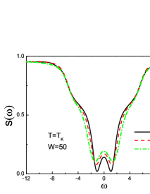
Figure 16: Shot noise spectrum in the Kondo regime, for several bias voltages ($\mu_{L}=-\mu_{R}=V/2$). Parameters: $\Gamma_{L}=\Gamma_{R}=\Gamma_{0}=0.5$, $\epsilon_{\uparrow}=\epsilon_{\downarrow}=\epsilon_{0}=-2$, and $U=6$. The Kondo temperature is determined by $T_{K}=\frac{U}{2\pi}\sqrt{\frac{-2U\Gamma_{0}}{\epsilon_{0}(U+\epsilon_{0})}}\exp[\frac{\pi\epsilon_{0}(U+\epsilon_{0})}{2U\Gamma_{0}}]$, from which we obtain $T_{K}=0.144$.

VI Concluding Remarks

In summary

, we have reviewed the formulation of particle-number($n$)-resolved master equation ($n$-ME) approach, and its application to quantum measurement and quantum transport in mesoscopic devices. The formalism under the (standard) second-order Born approximation is particularly simple and can be reliably applied to many practical problems. Importantly, the $n$-ME version is extremely appropriate for studying the shot noise and counting statistics (including also the large-deviation analysis), which encode additional dynamic information beyond the stationary current. The convenient application of the $n$-ME approach was illustrated by a couple of examples.

However, the second-order Born approximation does not fully capture the tunneling induced level-broadening and other multiple forward-backward-process induced correlation effects. Therefore, the first limitation is that the second-order ME to quantum transport is valid only for large bias voltage. On the other hand, for interacting systems (e.g., quantum dot or Anderson impurity), the second-order ME cannot describe the cotunneling and the nonequilibrium Kondo effect owing to the same reason. To overcome these limitations, higher-order expansions of the tunneling Hamiltonian are required, as performed by a variety of cases in literature Sch94 ; Sch96 ; Sch06 ; Yan080911 ; Yan2012 ; Wac05+10 ; CS11 ; Leeu09 ; Galp09 ; Galp10 ; KG13 .

We have therefore reviewed a newly proposed ME approach (and its $n$-resolved version) termed as SCBA-ME (under the self-consistent Born approximation when expanding the tunneling Hamiltonian). The basic idea is replacing the free (system only) Green’s function in the second-order self-energy operator by an effective propagator defined by the second-order ME. We found that the effect of this simple improvement is remarkable: it can recover not only the exact result of (any) noninteracting transport under arbitrary bias voltage but also describe the cotunneling and nonequilibrium Kondo effect in Coulomb interacting systems.

Finally, we mention that a similar idea of modifying the free propagator in the tunneling self-energy diagram by a dressed one was implemented also in a couple of recent studies Galp09 ; Galp10 ; KG13 . In Ref. KG13 , the specific Anderson impurity model was solved heavily based on a diagrammatic technique, but lacking a general formulation of basis-free master equation. In Refs. Galp09 ; Galp10 , owing to inappropriately treating the dressed propagator as a Markovian-Redfield generator, problems occurred as mentioned in the concluding remarks in Ref. Galp10 : “ $\cdots$ However, note that many important effects due to strong correlation between the molecule and contacts observed at low temperatures (e.g., Kondo) cannot be reproduced within our scheme. We find that our scheme becomes unreliable in the region of the parameters where coherences in the system eigenbasis (i.e., coherences introduced through nondiagonal elements of molecule-contact coupling matrix $\Gamma$) are bigger than the inter-level separation and on the order of the diagonal elements of the molecule-contact coupling matrix $\Gamma$”. Remarkably, the SCBA-ME approach reviewed in this work overcomes all these drawbacks.

Acknowledgments.

— The author is grateful to many former students and collaborators whose invaluable contributions constitute the main elements of this review article. Some of them are: Jinshuang Jin, Junyan Luo, Shikuan Wang, Hujun Jiao, Yonggang Yang, Jun Li, Feng Li, Yu Liu, Jing Ping, Ping Cui, Wenkai Zhang, Jiushu Shao, YiJing Yan, and Shmuel Gurvitz. This work was supported by the NNSF of China under No. 91321106 and the State “973” Project under Nos. 2011CB808502 & 2012CB932704.

References

- (1) H. Carmichael, An Open Systems Approach to Quantum Optics (Springer-Verlag, Berlin, 1993).
- (2) D. F. Walls and G. J. Milburn, Quantum Optics (Springer-Verlag, Berlin, 1994).
- (3) H. M. Wiseman and G. J. Milburn, Quantum Measurement and Control (Cambridge Univ. Press, Cambridge, 2009).
- (4) S.A. Gurvitz, Phys. Rev. B 56, 15215 (1997).
- (5) I.L. Aleiner, N.S. Wingreen, and Y. Meir, Phys. Rev. Lett. 79, 3740 (1997); Y. Levinson, Europhys. Lett. 39, 299 (1997); L. Stodolsky, Phys. Lett. B 459, 193 (1999); E. Buks, R. Schuster, M. Heiblum, D. Mahalu, and V. Umansky, Nature 391, 871 (1998); S. Pilgram and M. Büttiker, Phys. Rev. Lett. 89, 200401 (2002).
- (6) D. Mozyrsky and I. Martin, Phys. Rev. Lett. 89, 018301 (2002).
- (7) S.A. Gurvitz, L. Fedichkin, D. Mozyrsky, and G.P. Berman, Phys. Rev. Lett. 91, 066801 (2003).
- (8) M. H. Devoret and R. J. Schoelkopf, Nature (London) 406, 1039 (2000).
- (9) A. Shnirman and G. Schön, Phys. Rev. B 57, 15400 (1998).
- (10) Y. Makhlin, G. Schön, and A. Shnirman, Rev. Mod. Phys. 73, 357 (2001).
- (11) A. A. Clerk, S. M. Girvin, A. K. Nguyen, and A. D. Stone Phys. Rev. Lett. 89, 176804 (2002).
- (12) A.N. Korotkov, Phys. Rev. B 63, 085312 (2001); A.N. Korotkov and D.V. Averin, Phys. Rev. B 64, 165310 (2001); R. Ruskov and A.N. Korotkov, e-print cond-mat/0202303.
- (13) H.S. Goan, G.J. Milburn, H.M. Wiseman, and H.B. Sun, Phys. Rev. B 63, 125326 (2001); H.S. Goan and G.J. Milburn, Phys. Rev. B 64, 235307 (2001).
- (14) X.Q. Li, W.K. Zhang, P. Cui, J.S. Shao, Z.S. Ma, and Y.J. Yan, Phys. Rev. B 69, 085315 (2004) (LANL e-print cond-mat/0309574).
- (15) A. Shnirman, D. Mozyrsky, and I. Martin, e-print cond-mat/0211618.
- (16) T.M. Stace and S.D. Barrett, Phys. Rev. Lett. 92, 136802 (2004); e-print cond-mat/0309610.
- (17) D.V. Averin and A.N. Korotkov, e-print cond-mat/0404549; T.M. Stace and S.D. Barrett, e-print cond-mat/0406751.
- (18) X. Q. Li, P. Cui, and Y. J. Yan, Phys. Rev. Lett. 94, 066803 (2005).
- (19) X. Q. Li, J. Luo, Y. G. Yang, P. Cui, and Y. J. Yan, Phys. Rev. B 71, 205304 (2005).
- (20) S. Datta, Electronic Transport in Mesoscopic Systems (Cambridge University Press, New York, 1995).
- (21) H. Haug and A.-P. Jauho, Quantum Kinetics in Transport and Optics of Semiconductors (Springer-Verlag, Berlin, 1996).
- (22) Gurvitz S A, Prager Ya S. Microscopic derivation of rate equations for quantum transport. Phys Rev B, 1996, 53: 15932
- (23) S. A. Gurvitz, H. J. Lipkin, and Ya. S. Prager, Phys. Lett. A 212, 91 (1996).
- (24) Ya. M. Blanter and M. Büttiker, Phys. Rep. 336, 1 (2000); Quantum Noise in Mesoscopic Physics, edited by Yu. V. Nazarov (Kluwer, Dordrecht, 2003).
- (25) L. S. Levitov and G. B. Lesovik, JETP Lett. 58, 230 (1993); L. S. Levitov, H. W. Lee, and G. B. Lesovik, J. Math. Phys. 37, 4845 (1996).
- (26) W. Belzig and Yu. V. Nazarov, Phys. Rev. Lett. 87, 067006 (2001); W. Belzig and Yu. V. Nazarov, Phys. Rev. Lett. 87, 197006 (2001).
- (27) P. Samuelsson and M. Büttiker, Phys. Rev. Lett. 89, 046601 (2002); Phys. Rev. B 66, 201306 (2002).
- (28) S. Pilgram and P. Samuelsson, Phys. Rev. Lett. 94, 086806 (2005).
- (29) A. Thielmann, M. H. Hettler, J. König, and G. Schön, Phys. Rev. B 71, 045341 (2005); J. Aghassi, A. Thielmann, M. H. Hettler, and G. Schön, ibid. 73, 195323 (2006); A. Thielmann, M. H. Hettler, J. König, and G. Schön, Phys. Rev. Lett. 95, 146806 (2005).
- (30) W. Belzig, Phys. Rev. B 71, 161301(R) (2005).
- (31) B. R. Bulka, Phys. Rev. B 62, 1186 (2000).
- (32) A. Cottet, W. Belzig, and C. Bruder, Phys. Rev. Lett. 92, 206801 (2004).
- (33) Ya. M. Blanter, O. Usmani, and Yu. V. Nazarov, Phys. Rev. Lett. 93, 136802 (2004).
- (34) T. Novotny, A. Donarini, C. Flindt, and A.-P. Jauho, Phys. Rev. Lett. 92, 248302 (2004).
- (35) C. Flindt, T. Novotny, and A. P. Jauho, Europhys. Lett. 69, 475 (2005).
- (36) C. W. Groth, B. Michaelis, and C. W. J. Beenakker, Phys. Rev. B 74, 125315 (2006).
- (37) S. K. Wang, H. J. Jiao, F. Li, X. Q. Li, and Y. J. Yan, Phys. Rev. B 76, 125416 (2007).
- (38) S. Gustavsson, R. Leturcq, B. Simovič, R. Schleser, T. Ihn, P. Studerus, K. Ensslin, D. C. Driscoll, and A. C. Gossard, Phys. Rev. Lett. 96, 076605 (2006). T. Fujisawa, T. Hayashi, R. Tomita, and Y. Hirayama, Science 312, 1634 (2006).
- (39) Y. J. Yan, Phys. Rev. A 58, 2721 (1998).
- (40) J. Y. Luo, X. Q. Li, and Y. J. Yan, Phys. Rev. B 76, 085325 (2007).
- (41) J.-P. Eckmann and D. Ruelle, Rev. Mod. Phys. 57, 617 (1985); P. Gaspard, Chaos, Scattering and Statistical Mechanics (Cambridge University Press, Cambridge, England, 1998); H. Touchette, Phys. Rep. 478, 1 (2009).
- (42) D. Chandler, Introduction to Modern Statistical Mechanics (Oxford University Press, Oxford, 1987); N. Goldenfeld, Lectures on Phase Transitions and the Renormalization Group (Westview Press, Boulder, 1992).
- (43) J. P. Garrahan and I. Lesanovsky, Phys. Rev. Lett. 104, 160601 (2010).
- (44) S. K. Wang, H. J. Jiao, F. Li, X. Q. Li, and Y. J. Yan, Phys. Rev. B 76, 125416 (2007).
- (45) J. Li, Y. Liu, J. Ping, S. S. Li, X. Q. Li, and Y. J. Yan, Phys. Rev. B 84, 115319 (2011).
- (46) A. N. Korotkov, Phys. Rev. B 63, 085312 (2001); ibid 63, 115403(2001).
- (47) D. Mozyrsky, I. Martin, and M. B. Hastings, Phys. Rev. Lett. 92, 018303 (2004).
- (48) N. P. Oxtoby, H. M. Wiseman, and H. B. Sun, Phys. Rev. B 74, 045328 (2006).
- (49) S. A. Gurvitz and G.P. Berman, Phys. Rev. B 72, 073303 (2005).
- (50) A. N. Korotkov and D. V. Averin, Phys. Rev. B 64, 165310 (2001).
- (51) D. V. Averin, Phys. Rev. Lett. 88, 207901 (2002); A. N. Jordan and M. Büttiker, Phys. Rev. B 71, 125333 (2005).
- (52) S. K. Wang, J. S. Jin, and X. Q. Li, Phys. Rev. B 75, 155304(2007)
- (53) A. N. Jordan and M. Büttiker, Phys. Rev. Lett. 95, 220401 (2005).
- (54) H. J. Jiao, F. Li, S. K. Wang, and X. Q. Li, Phys. Rev. B 79, 075320 (2009).
- (55) A.W. Holleitner, et al, Phys. Rev. Lett. 87, 256802 (2001); A.W. Holleitner, et al, Science 297, 70 (2002).
- (56) J.C. Chen, A.M. Chang and M.R. Melloch, Phys. Rev. Lett. 92, 176801 (2004).
- (57) M. Sigrist, et al, Phys. Rev. Lett. 96, 036804 (2001).
- (58) J. König and Y. Gefen, Phys. Rev. Lett. 86, 3855 (2001); ibid, Phys. Rev. B 65, 045316 (2002).
- (59) I. Neder and E. Ginossar, Phys. Rev. Lett. 100, 196806 (2008).
- (60) F. Li, X. Q. Li, W. M. Zhang, and S. Gurvitz, Europhys. Lett. 88, 37001 (2009).
- (61) F. Li, H. J. Jiao, J. Y. Luo, X. Q. Li, and S. A. Gurvitz, Physica E 41, 1707 (2009).
- (62) Y. Cao, P. Wang, G. Xiong, M. Gong, and X. Q. Li, Phys. Rev. B 86, 115311 (2012).
- (63) P. Wang, Y. Cao, M. Gong, G. Xiong, and X. Q. Li, Europhys. Lett. 103, 57016 (2013).
- (64) P. Wang, Y. Cao, M. Gong, S. S. Li, and Xin-Qi Li, Phys. Lett. A 378, 937 (2014).
- (65) E. Majorana, Nuovo Cimento 14, 171 (1937).
- (66) F. Wilczek, Nat. Phys. 5, 614 (2009); M. Franz, Physics 3, 24 (2010).
- (67) A. Y. Kitaev, Physics-Uspekhi 44, 131 (2001).
- (68) R. M. Lutchyn, J. D. Sau, and S. Das Sarma, Phys. Rev. Lett. 105, 077001 (2010).
- (69) Y. Oreg, G. Refael, and F. von Oppen, Phys. Rev. Lett. 105, 177002 (2010).
- (70) J. D. Sau, R. M. Lutchyn, S. Tewari, and S. Das Sarma, Phys. Rev. Lett. 104, 040502 (2010).
- (71) J. D. Sau, S. Tewari, and S. Das Sarma, Phys. Rev. B 85, 064512 (2012).
- (72) L. Fu and C. L. Kane, Phys. Rev. Lett. 100, 096407 (2008).
- (73) J. Alicea, Phys. Rev. B 81, 125318 (2010).
- (74) V. Mourik, K. Zuo, S. M. Frolov, S. R. Plissard, E. P. A. M. Bakkers, L. P. Kouwenhoven, Science 1222360 (12 April 2012).
- (75) D. E. Liu and H. U. Baranger, Phys. Rev. B 84,201308 (2011).
- (76) C.J. Bolech and E. Demler, Phys. Rev. Lett. 98, 237002 (2007).
- (77) K. T. Law, P. A. Lee, and T. K. Ng, Phys. Rev. Lett. 103, 237001 (2009).
- (78) S. Tewari, C. Zhang, S. Das Sarma, C. Nayak, and D. H. Lee, Phys. Rev. Lett. 100, 027001 (2008).
- (79) L. Y. Chen and C. S. Ting, Phys. Rev. B 43, 4534 (1991).
- (80) J. S. Jin, J. Li, Y. Liu, X. Q. Li and Y. J. Yan, J. Chem. Phys. 140, 244111 (2014).
- (81) Y. Liu, J. S. Jin, J. Li, X. Q. Li and Y. J. Yan, Commun. Theor. Phys. 60, 503 (2013).
- (82) Y. Liu, J. S. Jin, J. Li, X. Q. Li, and Y. J. Yan, SCIENCE CHINA Physics, Mechanics& Astronomy 56, 1866 (2013).
- (83) H. Schoeller and G. Schön, Phys. Rev. B 50, 18436 (1994).
- (84) J. König, H. Schoeller, and G. Schön, Phys. Rev. Lett. 76, 1715 (1996); J. König, J. Schmid, H. Schoeller, and G. Schön, Phys. Rev. B 54, 16820 (1996).
- (85) A. Thielmann, M. H. Hettler, J. König, and G. Schön, Phys. Rev. Lett. 95, 146806 (2005).
- (86) J. S. Jin, X. Zheng, and Y. J. Yan, J. Chem. Phys. 128, 234703 (2008); X. Zheng, J. S. Jin, and Y. J. Yan, New J. Phys. 10, 093016 (2008); X. Zheng, J. S. Jin, S. Welack, M. Luo, and Y. J. Yan, J. Chem. Phys. 130, 164708 (2009).
- (87) Z. H. Li, N. H. Tong, X. Zheng, D. Hou, J. H. Wei, J. Hu, and Y. J. Yan, Phys. Rev. Lett. 109, 266403 (2012).
- (88) J. N. Pedersen and A. Wacker, Phys. Rev. B 72, 195330 (2005); Physica E 42, 595 (2010).
- (89) A. Croy and U. Saalmann, New J. Phys. 13, 043015 (2011).
- (90) P. Myöhänen, A. Stan, G. Stefanucci, and R. van Leeuwen, Phys. Rev. B 80, 115107 (2009).
- (91) M. Esposito and M. Galperin, Phys. Rev. B 79, 205303 (2009).
- (92) M. Esposito and M. Galperin, J. Phys. Chem. C 114, 20362 (2010).
- (93) J. Kern and M. Grifoni, Eur. Phys. J. B 86, 384 (2013).
- (94) R. D. Mattuck, A guide to Feynman diagrams in the many-body problem (Dover publications, New York, 1974).
- (95) D. C. Ralph and R. A. Buhrman, Phys. Rev. Lett. 72, 3401 (1994).
- (96) J. S. Jin, X. Q. Li, M. Luo, and Y. J. Yan, J. Appl. Phys. 109, 053704 (2011).
- (97) D. Goldhaber-Gordon, H. Shtrikman, D. Mahalu, D. Abusch-Magder, U. Meirav, and M. A. Kastner, Nature 391, 156 (1998).
- (98) S. M. Cronenwett, T. H. Oosterkamp, and L. P. Kouwenhoven, Science 24, 540 (1998). Cronenwett S M, Oosterkamp T H, Kouwenhoven L P. A Tunable Kondo Effect in Quantum Dots. Science, 1998, 24: 540
- (99) L. I. Glazman and M. Pustilnik, in Lectures notes of the Les Houches Summer School 2004 in “Nanophysics: Coherence and Transport”, edited by H. Bouchiat et al. (Elsevier, 2005), pp. 427-478.
- (100) T. K. Ng and P. A. Lee, Phys. Rev. Lett. 61, 1768 (1988).
- (101) S. Hershfield, J. H. Davies, and J. W. Wilkins, Phys. Rev. Lett. 67, 3720 (1991).
- (102) Y. Meir and N. S. Wingreen, Phys. Rev. Lett. 68, 2512 (1992).
- (103) Y. Meir, N. S. Wingreen, and P. A. Lee, Phys. Rev. Lett. 70, 2601 (1993).
- (104) D. C. Ralph and R. A. Buhrman, Phys. Rev. Lett. 72, 3401 (1994).
- (105) J. Paaske, A. Rosch, P. Wölfle, N. Mason, C. M. Marcus, and J. Nygard, Nature Phys. 2, 460 (2006).
- (106) M. Grobis, I. G. Rau, R. M. Potok, H. Shtrikman, and D.Goldhaber-Gordon, Phys. Rev. Lett. 100, 246601 (2008).
- (107) Z. H. Li, N. H. Tong, X. Zheng, D. Hou, J. H. Wei, J. Hu, and Y. J. Yan, Phys. Rev. Lett. 109, 266403 (2012).
- (108) T. Delattre et al, Nature Phys. 5, 208 (2009).
- (109) O. Zarchin, M. Zaffalon, M. Heiblum, D. Mahalu, and V. Umansky, Phys. Rev. B 77, 241303 (2008).
- (110) G. H. Ding and T. K. Ng, Phys. Rev. B 56, 15521(R) (1997).
- (111) A. Schiller and S. Hershfield, Phys. Rev. B 58, 14978 (1998).
- (112) T. Korb, F. Reininghaus, H. Schoeller, and J. König, Phys. Rev. B 76, 165316 (2007).
- (113) C. P. Moca, P. Simon, C. H. Chung, and G. Zarand, Phys. Rev. B 83, 201303(R) (2011).