THE INTERMEDIATE-MASS STAR FORMING REGION LYNDS 1340.
AN OPTICAL VIEW

Abstract

We have performed an optical spectroscopic and photometric search for young stellar objects associated with the molecular cloud Lynds 1340, and examined the structure of the cloud by constructing an extinction map, based on SDSS data. The new extinction map suggests a shallow, strongly fragmented cloud, having a mass of some 3700 M_☉. Longslit spectroscopic observations of the brightest stars over the area of L1340 revealed that the most massive star associated with L1340 is a B4 type, $\sim 5$ M_☉ star. The new spectroscopic and photometric data of the intermediate mass members led to a revised distance of $825^{+110}_{-80}$ pc, and revealed seven members of the young stellar population with $M\gtrsim 2$ M_☉. Our search for H$\alpha$ emission line stars, conducted with the Wide Field Grism Spectrograph $2$ on the $2.2$-meter telescope of the University of Hawaii and covering a $30\arcmin\times 40\arcmin$ area, resulted in the detection of 75 candidate low-mass pre-main sequence stars, 58 of which are new. We constructed spectral energy distributions of our target stars, based on SDSS, 2MASS, Spitzer, and WISE photometric data, derived their spectral types, extinctions, and luminosities from BVRIJ fluxes, estimated masses by means of pre-main sequence evolutionary models, and examined the disk properties utilizing the 2–24 µm interval of the spectral energy distribution. We measured the equivalent width of the H$\alpha$ lines and derived accretion rates. The optically selected sample of pre-main sequence stars has a median effective temperature of 3970 K, stellar mass 0.7 M_☉, and accretion rate of 7.6$\times 10^{-9}$ M_☉ yr^-1.

1 INTRODUCTION

Lynds 1340 is an isolated dark cloud at (l,b) = (130.1°,11.5°) (Kun, 2008), near the top of the Galactic molecular disk (see e.g. the wide-field 12 $\mu$m WISE Sky Survey Atlas (WSSA) image in Meisner & Finkbeiner, 2014). According to the first large-scale study of the region (Kun et al., 1994, hereinafter Paper I) L1340 is located at 600 pc from the Sun, and the blue reflection nebulosity DG 9 (Dorschner & Gürtler, 1968), illuminated by a few mid-B and early A-type stars (Paper I), suggest that it belongs to the class of the intermediate-mass star-forming regions (IM SFRs, Arvidsson et al., 2010; Lundquist et al., 2014) whose origin, evolution, and role in the Galactic star-forming history are not well studied. IM SFRs are not associated with H II zones, but illuminate blue reflection nebulae and excite the polycyclic aromatic hydrocarbon molecules of the environment, resulting in strong mid-infrared diffuse background. The ¹³CO observations of L1340 revealed a total mass of 1100 M_☉, some two orders of magnitude smaller than that of a typical giant molecular cloud. Three dense C¹⁸O clumps, L1340 A, L1340 B and L1340 C comprise some 85% of the total molecular mass. Three red and nebulous objects, RNO 7, RNO 8, and RNO 9 (Cohen, 1980), containing small groups of faint stars, are associated with the three clumps, respectively. Ten dense cores were identified in L1340 through a large-scale NH₃ survey by Kun, Wouterloot, & Tóth (2003, hereinafter Paper II), with masses and kinetic temperatures halfway between the values obtained for the ammonia cores in Taurus and Orion (Jijina et al., 1999). Thirteen H$\alpha$ emission objects ([KOS94] HA 1–[KOS94] HA 13) were found by Kun et al. (1994), and 14 ones (RNO 7 HA 1–14), concentrated in the small nebulous cluster RNO 7 by Magakian, Movsessian, & Nikogossian (2003). Herbig–Haro objects HH 487, HH 488, HH 489, HH 671, and their driving sources are reported in Kumar, Anandarao, & Yu (2003) and Magakian et al. (2003).

To explore the nature of interstellar processes, leading to star formation in such an environment, and the role of feedback from young intermediate-mass stars on their natal cloud, the structure of the cloud and the census of the young stellar object (YSO) population have to be assessed. The low sensitivity of the photographic H$\alpha$ survey presented in Paper I, and the small angular coverage of the more sensitive H$\alpha$ survey by Magakian et al. (2003) suggest that most of the classical T Tauri stars associated with L1340 are still undiscovered. In order to identify the YSO population of L1340 we performed a wide-field slitless grism survey for H$\alpha$ emission stars, and low-resolution, optical longslit spectroscopic observations of the bright stars of the region, illuminating reflection nebulae. To derive the luminosities of the target stars and examine their spectral energy distributions (SEDs) we supplemented our observations with optical photometric data available in the SDSS data base, as well as with 2MASS, Spitzer, and WISE infrared photometric data. To study the cloud structure we constructed a new extinction map using SDSS data. The results complement our recent infrared search for the YSO population of the cloud, based on our own observations and public data bases (Kun et al., 2016, hereinafter Paper III). Our data and analysis are described in Sect. 2 and 3, respectively. The results are presented in Sect. 4, and discussed in Sect. 5. A brief summary is given in Sect. 6.

2 DATA

2.1 Longslit Spectroscopy

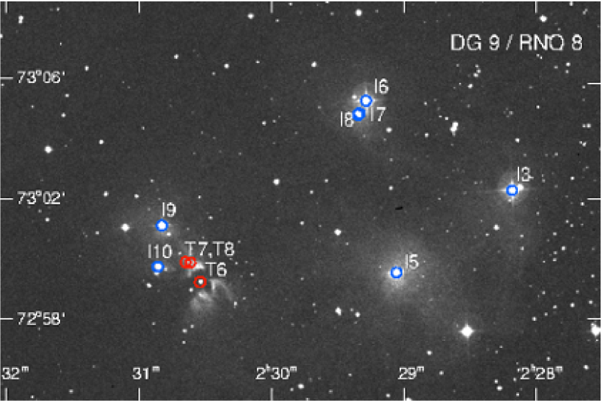
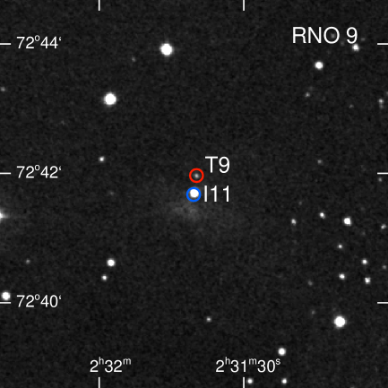
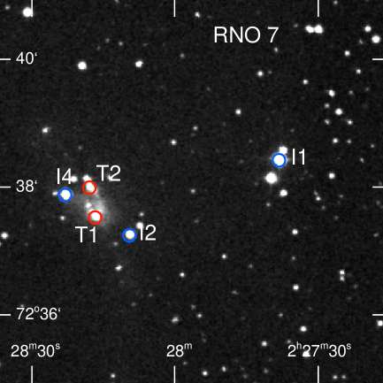
Figure 1: Targets of our spectroscopic observations, marked on the DSS2 blue images. Top: Nebulous stars associated with DG 9 and RNO 8; Bottom right: Blue and nebulous stars observed in the RNO 7 region; Bottom left: the stars in the RNO 9 region. Numbering of the stars are same as in Table 1. Blue and red circles indicate blue and red objects, respectively.

To identify and classify the most luminous optically visible young stars associated with L1340 we obtained low and intermediate resolution optical spectra of seven stars, associated with the extended reflection nebulosity DG 9 (Dorschner & Gürtler, 1968), three stars in the region of the nebulous cluster RNO 7, three stars belonging to the small, red nebulosity RNO 8, and two stars in the RNO 9 region (Cohen, 1980), as well as of six further [KOS94] HA stars. Furthermore, we included in the target list two stars projected on the RNO 7 cluster and much brighter and bluer than typical cluster stars. The target stars whose association with the cloud is evidenced by reflection nebulae are shown in Fig. 1. The star No. 1, located east of RNO 7 (lower right panel of Fig. 1, 2MASS 02273807+7238267) was selected due to its associated 8-$\mu$m nebulosity (Paper III).

We observed the optical spectra of 23 stars utilizing several instruments, namely CAFOS with the G–100 grism, installed on the 2.2-m telescope of the Calar Alto Observatory, FAST on the 1.5-m telescope of the Fred Lawrence Whipple Observatory (Fabricant et al., 1998), ALFOSC with grism 8 on the Nordic Optical Telescope in the Observatorio del Roque de los Muchachos in La Palma, and the low-resolution slit spectrograph operated on the 1-m RCC telescope of the Konkoly Observatory. The log of the spectroscopic observations is shown in Table 1. We reduced the data following the standard IRAF procedures (see further details in Kun et al., 2009).

2.2 Slitless Grism Spectroscopic Observations

We observed L1340 with the Wide Field Grism Spectrograph 2 (WFGS2), installed on the University of Hawaii 2.2-meter telescope, on 2011 January 1, October 15, 16, and 18, and 2012 August 10. We used a 300 line mm^-1 grism, blazed at 6500 Å, and providing a dispersion of 3.8 Å pixel^-1 and a resolving power of 820. The narrow band H$\alpha$ filter had a 500 Å  passband centered near 6515 Å. The detector for WFGS2 is a Tektronix $2048\times 2048$ CCD, whose pixel size of 24 $\mu$m  corresponds to 0.34 arcsec on the sky. The field of view is $11.5\arcmin\times 11.5\arcmin$. We covered an area of $30\times 40$ arcmin, centered on RA(2000)$=2^{\mathrm{h}}30^{\mathrm{m}}$ and Dec(2000)$=72\arcdeg 48\arcmin$, with a mosaic of 12 overlapping fields. For each field, we took a short, 60 s exposure in order to detect the H$\alpha$ line in bright stars, and three frames of 300 s exposure.

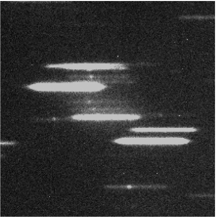
Figure 2: Part of the WFGS2 image showing the H$\alpha$ emission stars of the RNO 7 cluster.

Bias subtraction and flat-field correction of the images were done in IRAF. Then we used the FITSH, a software package for astronomical image processing (Pál, 2012) to remove cosmic rays, coadding the long-exposure images, identify the stars on the images, and transform the pixel coordinates into equatorial coordinate system. As an example of the reduced and coadded images, the central part of the RNO 7 cluster can be seen in Fig. 2.

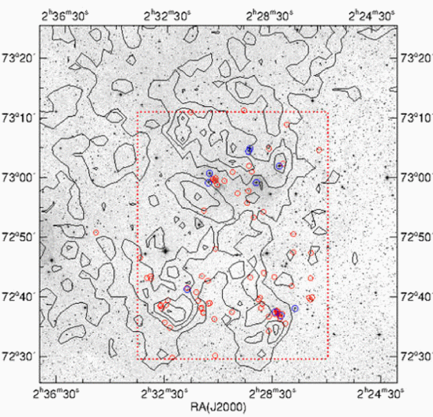
Figure 3: Positions of the H$\alpha$ emission stars (red circles) and stars earlier than F5 (blue circles) on the DSS2 red image of the 1 square degree region centered on RA(J2000.0)=$2^{\mathrm{h}}30^{\mathrm{m}}30^{\mathrm{s}}$, Dec(J2000.0)=$+72\arcdeg 56\arcmin$. Extinction contours of $A_{\mathrm{V}}=1,2,3\ldots$ are overplotted. The dotted rectangle outlines the area covered by the WFGS2 observations.

We found 75 stars with H$\alpha$ emission by examining the images visually. We determined their equatorial coordinates by matching our images with the 2MASS (Cutri et al., 2003) image of the field. We could associate all but two emission sources with 2MASS point-sources unambiguously within $1\arcsec$. Therefore we use 2MASS designations of the stars for equatorial coordinates. For the two stars missing from the 2MASS All Sky Catalogue we use their SDSS DR9 identifiers. One of these stars, SDSS9 J022856.42+724019.2, situated at some 2″ from another, brighter H$\alpha$ emission star, 2MASS 02285635+7240171 (SDSS9 J022856.34+724017.1), has no counterpart in any of the 2MASS, WISE, and Spitzer data. The other one, SDSS9 J022932.32+725503.3, although too faint for the 2MASS, can be identified in the AllWISE data base and Spitzer images. We detected H$\alpha$ emission from 18 stars, previously identified as H$\alpha$ emission objects by Kun et al. (1994) and Magakian et al. (2003), and from the hypothetical exciting source of the Herbig–Haro object HH 488 (HH 488 S, Kumar et al., 2003). The equivalent width of the H$\alpha$ emission line EW(H$\alpha$) and its uncertainty were computed in the manner described by Szegedi-Elek et al. (2013). Due to the faint continuum or overlapping spectra we could not measure EW(H$\alpha$) in the spectra of six stars. Table 2 lists the 2MASS designations, measured EW(H$\alpha$), and cross-identifiers of the H$\alpha$ emission stars of L1340, consisting of the 75 stars identified in the WFGS2 images and the two ones identified during the longslit observations but outside of the field of view of the WFGS2 observations. Figure 3 shows the positions of the H$\alpha$ emission stars, overplotted on the DSS2 red image of the region.

2.3 Photometric Data

Spitzer

L1340 was observed by the Spitzer Space Telescope using Spitzer’s Infrared Array Camera (IRAC; Fazio et al., 2004) on 2009 March 16 and by the Multiband Imaging Photometer for Spitzer (MIPS; Rieke et al., 2004) on 2008 November 26 (Prog. ID: 50691, PI: G. Fazio). The IRAC observations covered $\sim 1$ deg² in all four bands. The centers of the 3.6 and 5.8 $\mu$m images are slightly displaced from those of the 4.5 and 8 $\mu$m images, therefore part of the clump L1340 C is outside of the 4.5 and 8 $\mu$m images. Moreover, the 24 and 70 $\mu$m images do not cover the southern half of L1340 A. A small part of the cloud, centered on RNO 7, was observed in the four IRAC bands on 2006 September 24 (Prog. ID: 30734, PI: D. Figer). Each of our longslit spectroscopic target stars are located within the field of view of the Spitzer observations. All but two of the 75 H$\alpha$ emission stars detected by the WFGS2 are within the field of view of the 3.6 and 5.8-$\mu$m  images, albeit 14 of them are outside of the 4.5 and 8-$\mu$m images. We performed IRAC and MIPS photometry of the target stars by the procedure described in Kun et al. (2014).

AllWISE

All but eight of the H$\alpha$ sources have counterparts in the AllWISE Source Catalog (Wright et al., 2010). The WISE  images of L1340 reveal bright diffuse background at 12 and 22 µm (see Paper III). Point source fluxes in the W3 and W4 bands may therefore be contaminated by the diffuse radiation, originating from the environment. We applied the criteria, set by Koenig & Leisawitz (2014), to discriminate real point source fluxes and fake sources, resulting from background-contaminated data in the W3 and W4 bands. We found reliable WISE 22-$\mu$m fluxes for five H$\alpha$ emission stars, not observed or not detected by MIPS at 24-$\mu$m, allowing us to classify the SEDs of these stars.

SDSS

L1340 is situated within Stripe 1260 of the SEGUE survey (Yanny et al., 2009). Each of our target stars has a counterpart in the SDSS Data Release 9 (Ahn et al., 2012) within 1″ of the 2MASS position. We include the optical data points into the SEDs of the stars, and use them for estimating their extinctions and spectral types. To compare the color indices with those of the spectral sequence of pre-main sequence stars, published by Pecaut & Mamajek (2013), we transformed the ugriz magnitudes into the Johnson–Cousins UBVR_CI_C system, using the equations given in Ivezić et al. (2007, for BVR_CI_C) and Jordi et al. (2006, for U). Furthermore, we use SDSS data for constructing an extinction map of the cloud.

Photometric data of the target stars are presented in Tables A1 and A2 of Appendix A. Table A1 lists the UBVR_CI_C and 2MASS JHK_s magnitudes, and Table A2 contains the Spitzer [3.6], [4.5], [5.8], [8.0], [24], and [70.0] magnitudes, and AllWISE [3.4], [4.6], [12], and [22] magnitudes for the optically selected candidate young stars associated with L1340.

3 ANALYSIS

3.1 Spectral Classification

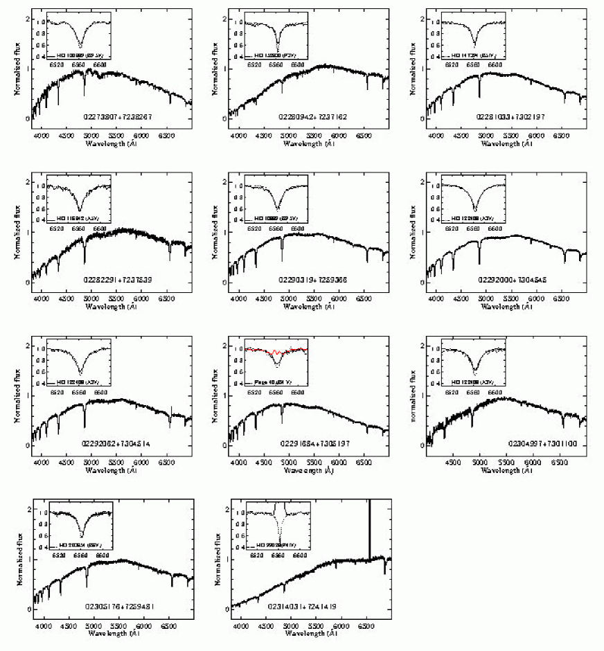
Figure 4: Spectra of the observed stars earlier than F5. In the inset the region of the H$\alpha$ line is magnified. The red line in the inset of the star 02291684+7305197 shows the H$\alpha$ line observed on 1999 August 7, and the black line shows the spectrum detected on 2004 November 6. For comparison the H$\alpha$ line of a standard star of the same type is drawn with a dotted line.

We analysed our longslit spectra using the ‘splot’ task of IRAF. The spectral types of the stars were determined by comparing the absorption features with those in a number of standard star spectra found in the spectrum library of Jacoby, Hunter, & Christian (1984), and following the criteria described in Hernández et al. (2004) and Gray & Corbally (2009). Spectra of the stars earlier than F5 are shown in Fig. 4, and their spectral types are listed in Table 3. We examined the H$\alpha$ lines in these spectra for the presence of a possible emission component, overlying the photospheric H$\alpha$ absorption line. The inset in each panel shows the H$\alpha$ line of the target star together with that of a standard star of the same spectral type. We estimate the accuracy of the spectral types of these stars as $\pm 1$ subclass. Spectra of the observed H$\alpha$ emission stars are displayed in Fig. 5. The classification of these stars is less accurate due to their low brightness and non-photospheric line and continuum emission. The spectral types of these stars are listed in Table 4. We adopt a two-subclass uncertainty, which is supported by the comparison of the results with those obtained from the SEDs (see Sect. 3.2).

3.2 Spectral Energy Distributions

The available SDSS, 2MASS, Spitzer, and WISE photometric data allowed us to plot the SEDs of the observed stars over the 0.36–24 (70) µm wavelength region. Having the spectral types of the longslit target stars determined, we dereddened their observed SEDs according to the normal interstellar reddening law ($R_{\mathrm{V}}=3.1$) of Cardelli, Clayton, & Mathis (1989) to match the photospheric SED of the given spectral type, defined by the color indices tabulated by Pecaut & Mamajek (2013).

SEDs of the H$\alpha$ emission stars, detected by WFGS2, were also constructed using all photometric data. Akari IRC fluxes (Ishihara et al., 2010) at 9.0 and 18.0 $\mu$m are also included when available. We estimated the spectral type and the extinction of each target star by comparing visually the optical–near infrared SED (from the B to the J band) with those of a grid of reddened photospheres, using the reddening-free color indices of Pecaut & Mamajek (2013), the extinction law of Cardelli et al. (1989), and the $A_{\mathrm{V}}\geq 0.5$ mag restriction (Kun et al., 2003). We found the best fit of the photometry and photospheric colors using the reddening law $R_{\mathrm{V}}=3.1$ for $A_{\mathrm{V}}\lesssim 2.0$, and with $R_{\mathrm{V}}=5.5$ for $A_{\mathrm{V}}\gtrsim 2.0$. Similar dependence of the extinction law on the line-of-sight $A_{\mathrm{V}}$ was reported by Allen et al. (2014) for the Cepheus OB3 star-forming region. We estimate the accuracy of the resulting spectral types and extinction as $\pm 2$ subclass and $\pm 0.5$ mag, respectively.

We classified the infrared excesses of the H$\alpha$ emission stars based on their dereddened SED slopes, $\alpha=d\log(\lambda F(\lambda))/d\log\lambda$, over the 2–24 (22) $\mu$m interval (WISE data were used for classification when no Spitzer data were available). According to the canonical classification scheme (Lada, 1991; Greene et al., 1994) Class I protostars are characterized by $\alpha>0.3$, $-0.3\leq\alpha\leq 0.3$ indicates Flat SED sources, near the boundary between the protostellar and pre-main sequence evolutionary phases, whereas classical T Tauri stars have Class II slopes with $-0.3>\alpha\geq-1.6$. Class III young stars with $\alpha\leq-1.6$ are pre-main sequence stars with very weak or no infrared excess. Class II SEDs then can be further divided into the primordial (II P), pre-transitional/transitional (II T), and weak or ‘anemic’ (II A) subclasses (Evans et al., 2009), based on the details of the SED over the 2–24 µm  wavelength interval, compared to those of the median SED of the benchmark sample of T Tauri stars of the Taurus region. We constructed the Taurus median SED using Furlan et al.’s (2006) data, established for K5–M2 type stars over the 1.25 $\micron\ \leq\lambda\leq 34.00$ µm  region, and those of D’Alessio et al. (1999) for optical and far-infrared wavelengths. A circumstellar disk is primordial if the SED does not drop below the Taurus median band; it is an evolved pre-transitional or transitional disk if the SED is below the Taurus median band in the near-infrared, and starts rising in the mid-infrared, whereas the SED of a weak or anemic disk is below the Taurus band over the whole observed infrared region. Since the evolutionary processes leading to the II A and II T subclasses may be different, their occurrence and properties within the same star-forming environment may bear information on their origin.

3.3 Hertzsprung–Russell Diagram

Having determined spectral classes and extinctions we calculated the bolometric luminosities of the target stars from the extinction-corrected V, $I_{\mathrm{C}}$, and J magnitudes separately, using the bolometric corrections and color indices tabulated by Pecaut & Mamajek (2013), and adopting the new distance of 825 pc (see Sect. 4.1). Then we took the average of the luminosities obtained from the three photometric bands. To find the positions of our target stars in the $\log T_{\mathrm{eff}}$ – $\log L$ plane, effective temperatures, corresponding to their spectral types, were also adopted from Pecaut & Mamajek (2013). To estimate the masses and ages of our target stars, we applied evolutionary tracks and isochrones from Siess et al.’s (2000) pre-main sequence evolutionary models. The errors of $T_{\mathrm{eff}}$ originate from the uncertainty of the spectral classification, and the errors of the luminosities were propagated from the photometric errors, and uncertainties of distance, extinction and bolometric correction.

3.4 Extinction Mapping

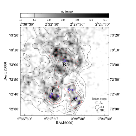
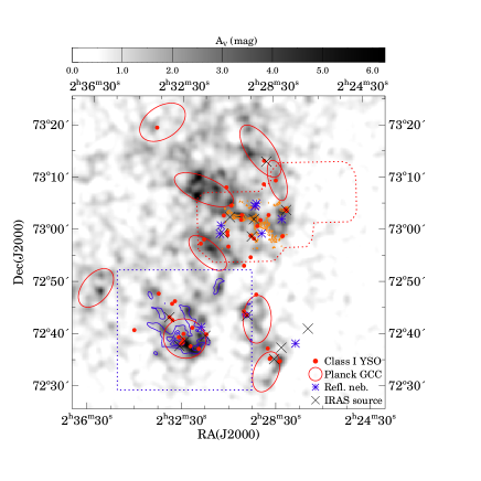
Figure 6: Visual extinction map of L1340, determined from star counts in the SDSS DR9. (a) Thin solid black contours show the integrated intensity contours of the ¹³CO. The lowest contour and the increment are 0.56 K km s^-1. The red dash-dotted lines indicate the C¹⁸O contours $T_{A}=0.30(\sim 5\,\sigma)$, and 0.60 K. Blue circles show the positions of NH₃ cores (Paper II). (b) Comparison of the extinction map with various dust-tracers. The lowest contour is at $A_{\mathrm{V}}=1$ mag, and the increment is 1 mag. Yellow contours indicate 850 $\mu$m continuum detected by SCUBA. Contours are at 25, 50,, and 100 mJy beam^-1. Blue contours show the 500-$\mu$m emission of the cold dust, measured by the SPIRE instrument of the Herschel Space Observatory (Juvela et al., 2012). The levels are at 30, 50, and 70 Jy pixel^-1. Ellipses indicate the positions and sizes of the Planck cold cores. Reflection nebulae and embedded YSOs are also overplotted. Meaning of the symbols are shown in the lower right corner. The red dotted line indicates the approximate boundary of the SCUBA observations, and the blue dotted line borders the Herschel 500 $\mu$m image.

The high sensitivity SDSS data and the improved census of the YSO population of L1340 allow us to refine the picture of the dust column density structure of L1340, compared to available extinction maps of the region (Paper II, Rowles & Froebrich, 2009; Dobashi, 2011). We constructed an extinction map, applying the classical method of star counts (Dickman, 1978) on the SDSS DR9 data set. We repeated the procedure that was applied on the DSS2 data in Paper II. We counted the stars on 90-arcsec sized squares, whose centres were distributed on a regular grid with step of 15″. The number of stars with V $\leq 25$ mag within a 1 square degree area was 30562. We omitted all classified galaxies, and removed each star with V $<14$ mag as probable foreground object. Furthermore, we removed each identified candidate YSO, both the H$\alpha$ emission stars and the color-selected pre-main sequence stars (Paper III). The off-cloud reference area was a $6\arcmin\times 6\arcmin$ field centered at $RA(2000)=34.4779\arcdeg,D(2000)=+72.993\arcdeg$, containing 499 stars. The resulting $A_{\mathrm{V}}$ map then was boxcar-smoothed to reduce the scatter. The uncertainty of the extinction of a pixel, derived by the formula given in Dickman (1978) and depending on the pixel value itself, extends from $\sim 0.4$ mag in the low extinction areas (between 0–1 mag) to 1.4 mag near the extinction peaks. The resulting $A_{\mathrm{V}}$ map can be seen in Fig. 6.

4 RESULTS

4.1 Revised Distance

Main-sequence stars illuminating reflection nebulae are excellent distance indicators of interstellar clouds. The distance of L1340, given in Paper I, was determined using objective-prism spectral classes and photoelectric UBV magnitudes of three stars of L1340 B, associated with reflection nebulae (stars 3, 5, and 6 in Table 1, denoted in Paper I as R1, R2, and R3, respectively). This method resulted in $660\pm 30$ pc, and it was averaged with the lower value of 560 pc, suggested by a Wolf diagram, to 600 pc. We note that, in addition to the limited precision of spectral classification from very low dispersion spectra, the photoelectric magnitudes of some measured stars were contaminated by the light from visual companions, biasing the result toward a smaller distance. The new spectroscopic and photometric data allow us to refine the distance determination of L1340.

The results of our spectral classification, listed in Table 3, show that the two most luminuous stars associated with L1340 are the B5 type star No. I3 and the B4 type No. I6. Both stars were classified as B5 type in Paper I. The new spectra show that the He I lines are slightly stronger and the He I $\lambda\,4471$ to Mg I $\lambda\,4481$ ratio is higher in the spectrum of the latter star, suggesting an earlier type. Due to the short evolutionary time scales of such stars both of them were most probably born in L1340, and are located on the zero-age main sequence (ZAMS) of the Hertzsprung–Russell diagram. The effective temperatures of these spectral types, according to Pecaut & Mamajek (2013), are 15700 K and 16700 K, respectively, and the luminosities on the ZAMS, according to the intermediate-mass pre-main sequence evolutionary models of Palla & Stahler (1993), are 458 $L_{\sun}$ and 670 $L_{\sun}$, respectively. Applying the unreddened color indices and bolometric corrections, tabulated by Pecaut & Mamajek (2013), we obtain distances of 855 pc and 794 pc for the two stars, respectively. We adopt the new distance of 825 pc in the rest of this paper. A $\pm 1$ subclass scatter of the spectral types results in the distance range $750\lesssim D\lesssim 940$ pc. The recent paper of Green et al. (2015) suggests similar distance of the dark clouds at the Galactic coordinates of L1340.

4.2 Cloud Structure and Clump Masses

The new $A_{\mathrm{V}}$ map of L1340 is shown in Fig. 6. To compare the distribution of the gas and dust, ¹³CO  and C¹⁸O contours (Paper I) are drawn and positions of the ammonia cores are overplotted in the left panel (a). The right panel (b) compares the new extinction map with the distribution of various dust-indicators. We have drawn the contours of the 850-$\mu$m emission, available for the clump L1340 B in the SCUBA Legacy Catalogues (Di Francesco et al., 2008), and 500-$\mu$m emission contours, measured by Herschel SPIRE for L1340 C (Juvela et al., 2012), as well as positions of stars illuminating reflection nebulae (Paper I), Planck Galactic cold cores (PGCCs, Planck Collaboration, 2015), and embedded protostars (Paper I, Paper III).

Our extinction map saturates at $A_{\mathrm{V,max}}=6.7$ mag. The extinction exceeds this value on 2 pixels within the area of clump  A, on 50 pixels within clump B, and 27 pixels in clump C. The column density at these positions is close to the critical lower limit of $A_{\mathrm{V}}\approx 8$ mag found for star-forming clumps in several molecular clouds (e.g. Molinari et al., 2014, and references therein).

The overall structure and the mean $A_{\mathrm{V}}$ are compatible with those obtained by Rowles & Froebrich (2009) and Dobashi (2011), based on 2MASS color excesses. We find the mean extinction $\langle A_{\mathrm{V}}\rangle=1.87$ mag for the region of the cloud within the $A_{\mathrm{V}}=1.0$ mag contour. The same average is 1.85 mag for Rowles & Froebrich’s (2009) extinction map, and 1.63 for the map of Dobashi (2011) (for the offset of both all-sky extinction maps see Rowles & Froebrich, 2009). A conspicuous difference is that, whereas the most opaque spots of our map are found in the largest clump B, the color index-based method indicates the maximum extinction at the position of the cluster RNO 7. The large median 2MASS  color indices at the position of RNO 7, leading to the high apparent extinction, may be caused by the large number of unidentified YSOs (Paper III). Another difference is that the maximum $A_{\mathrm{V}}$, derived from the color excesses, is 6.43 mag, whereas a few small, even darker regions can be detected in the map based on SDSS data.

Comparison of ¹³CO and $A_{\mathrm{V}}$ shows that the three clumps L1340 A, B, and C, revealed by the ¹³CO data, fragment into dark knots with typical sizes of a few arcminutes in the extinction map. In particular, the central region of L1340 B contains a conspicuous chain of dark spots, comparable in angular size with the resolution of the map, and also apparent in the 850 $\mu$m emission.

We estimated the mass of the cloud and its clumps using the extinction map. Assuming $N(HI+2H_{2})=1.9\times 10^{21}\times A_{\mathrm{V}}$, 36% helium and 1% dust mass, we obtain $M\approx 3700$ M_☉ for the cloud material above $A_{\mathrm{V}}=1.0$ mag, corresponding to the column density $N(HI+2H_{2})\gtrsim 0.94\times 10^{21}$ cm^-2. This part of the cloud covers an area of some 90 pc², and roughly coincides with the region detected in ¹³CO. Scaling the mass of 1100 M_☉, obtained from the ¹³CO observations, to 825 pc we obtain 2080 M_☉, demonstrating that the ¹³CO emission saturates at lower column density than the $A_{\mathrm{V}}$ map.

We estimated the masses of the clumps by summarizing the column densities for the regions above $A_{\mathrm{V}}=1.8$ mag, where the clumps separate. Table 5 lists the average sizes (square root of the area above the threshold), mean and maximum $A_{\mathrm{V}}$, and masses of the three clumps, adopting the distance of 825 pc.

Nine Planck Galactic cold cores are projected near extinction peaks, suggesting their physical relation to L1340. One of them, PGCC G130.38+11.26 was included in the detailed Herschel study by Juvela et al. (2012). Assuming a distance of 810 pc they derived a mass of 404 M_☉  for a region of 0.94 pc (4′) in diameter. Comparison of this result with those in Table 5 supports that the mass derived from the dust emission is compatible with that obtained from the extinction.

4.3 Intermediate-mass Young Stars

4.3.1 Stars Earlier than F5

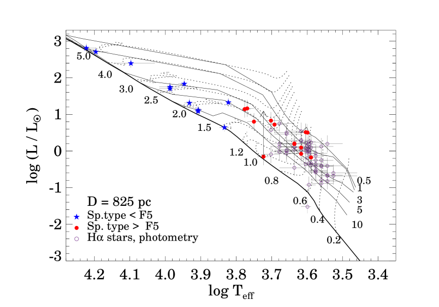
Figure 10: Hertzsprung–Russell diagram of the candidate young stellar population of L1340. Blue star symbols indicate the stars earlier than F5, red filled circles show those later than F5, listed in Table 1. Open circles indicate sources whose spectral types were derived from photometric data. Evolutionary tracks (dotted lines) and 0.5, 1, 3, 5, 10 million year isochrones (thin solid lines), and the main sequence (thick solid line) are from Siess et al. (2000). The stellar bolometric luminosities were calculated for a distance of 825 pc.

We identified 11 stars earlier than F5, projected on the surface of the molecular cloud. We expect to find optically visible intermediate mass ($M\gtrsim 2$ $M_{\sun}$) members of the YSO population of L1340 among these stars. The SEDs of these 11 stars, including all available photometric data, are shown in Fig. 7. The photospheric SEDs, matched to the extinction-corrected data at the $I_{\mathrm{C}}$  and J bands are also plotted. Spectral types, extinctions, effective temperatures, and luminosities of these stars are listed in Table 3, and they are plotted with blue star symbols in the Hertzsprung–Russell diagram in Fig. 10.

Five stars, Nos. I1, I5, I9, I10, and I11 in Table 3, are located above the ZAMS. These stars appear to be 1–3 million year old stars of 2–3 M_☉ mass. Figures 4 and 7 suggest that most of these stars lack emission lines and infrared excesses, characteristic of Herbig Ae/Be stars. The only obvious exception is star No. I11, an F4-type star associated with RNO 9, exhibiting both infrared excess and strong H$\alpha$ emission. Moreover, a weak emission component can be seen in the H$\alpha$ line of the B8-type star No. 10, and the B4-type star No. I6 exhibited H$\alpha$ emission in the spectrum recorded on 1999 Aug 7 (drawn by red line in Fig. 4). The mass of this latter star, estimated from the position on the zero-age main sequence, is about 5 M_☉. The two non-nebulous target stars projected on RNO 7 (Nos. I2 and I4) are located on the ZAMS at the distance of the cloud, like Nos. I7 and I8, members of a visual double embedded in the DG 9 nebula.

4.3.2 Intermediate-mass T Tauri Stars

Figure 10 suggests that seven of the brightest H$\alpha$ emission stars, (Nos. T1, T4, T8, T10, and T12 in Table 4, as well as Nos. 19 and 20 in Table 6) are as massive as 2–2.5 M_☉. According to the overplotted evolutionary tracks these stars are in a short-lived phase of their pre-main sequence evolution, and evolving toward higher temperatures and luminosities they will become either Herbig Ae stars or normal late B–early A-type stars (Herbig, 1994; Calvet et al., 2004).

A candidate embedded intermediate-mass young star is the central star of the optical nebulosity RNO 8, associated with IRAS 02259+7246 (No. T6 in Table 4 and No. 44 in Table 6). Its position near the ZAMS suggests that, at optical wavelengths we observe its photospheric spectrum scattered from the outer disk atmosphere, being thereby strongly attenuated (De Marchi et al., 2013). If we compute the bolometric luminosity of this source by integrating the whole available SED, and assume that the infrared fluxes originate from reprocessed starlight, the star will move upwards in the HRD, to the position indicated by an arrow in Fig. 10, suggesting a young star of some 2–2.5 M_☉.

4.4 The Classical T Tauri Population

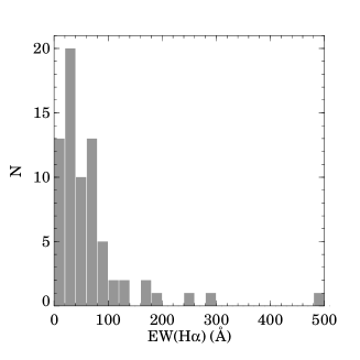
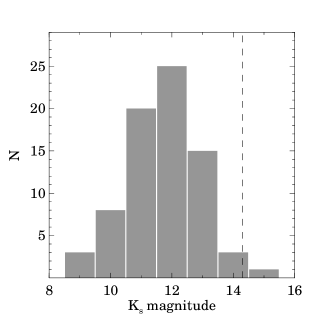
Figure 8: Histogram of the H$\alpha$ equivalent widths (left) and 2MASS K_s magnitudes of the H$\alpha$ emission stars. The vertical dashed line indicates the 2MASS K_s limiting magnitude.

The H$\alpha$ emission stars are candidate classical T Tauri stars (CTTSs) born in Lynds 1340. Twelve target stars of the longslit observations exhibited emission spectra characteristic of classical T Tauri stars. In addition to eight [KOS94] HA stars we detected H$\alpha$ emission in the spectra of three stars associated with the RNO 8 nebulosity, and in that of a faint star next to the F4 type pre-main sequence star RNO 9, referred to as RNO 9 B in Table 1. The derived spectral types and measured equivalent widths of the H$\alpha$ line are shown in Table 4. Ten of these stars are located within the boundaries of the WFGS2 observations, and were detected as H$\alpha$ emission stars in the WFGS2 images. To compare the equivalent widths measured with different methods, we list the EW(H$\alpha$), measured in the WFGS2 spectra of these stars, in the last column of Table 4. The comparison suggests no systematic difference between the equivalent widths measured in the slitless and longslit spectra. The left panel of Fig. 8 shows the histogram of the EW(H$\alpha$) of the 77 emission line stars, detected during the WFGS2 and longslit observations. Most of the measured equivalent widths are between 10 and 100 Å, typical for classical T Tauri stars (e.g Fernández et al., 1995; Reipurth, Pedrosa, & Lago, 1996). These strong emission lines originate from magnetospheric accretion and accretion-related winds (e.g. Muzerolle et al., 1998). The highest value (496 Å) belongs to the eruptive star V1180 Cas (Kun et al., 2011), and the next highest one (280 Å) was detected in HH 488 S (Kumar et al., 2003). EW(H$\alpha$)$<10$ Å were measured in the spectra of not more than two stars. The histogram of the $K_{\mathrm{s}}$ magnitudes of the H$\alpha$ emission stars is displayed in the right panel of Fig. 8.

4.4.1 Spectral Energy Distributions

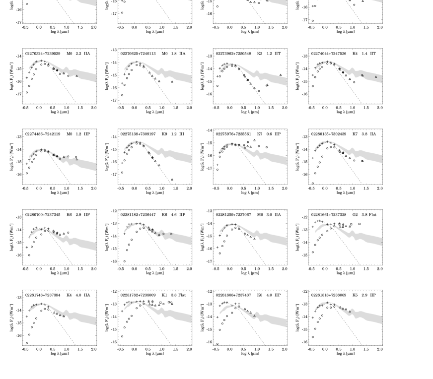
Figure 9: SEDs of the H$\alpha$ emission stars. Open circles show the SDSS, 2MASS, and WISE data, and triangles result from our Spitzer photometry. Open squares indicate Akari IRC fluxes. Plusses indicate the dereddened SED, and the dashed line shows the photospheric SED of the spectral type, obtained by fitting a model to the data (see the text). The gray shaded area indicates the median SED of the T Tauri stars of the Taurus star-forming region (D’Alessio et al., 1999). 2MASS identifiers, spectral types, and $A_{\mathrm{V}}$ extinctions, derived from photometric data, as well as the SED class are indicated at the top of each panel.

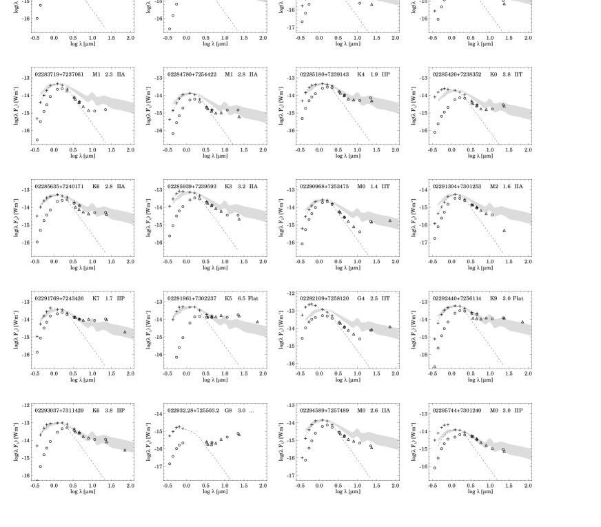
Figure 9: SEDs of the H$\alpha$ emission stars (continued.)

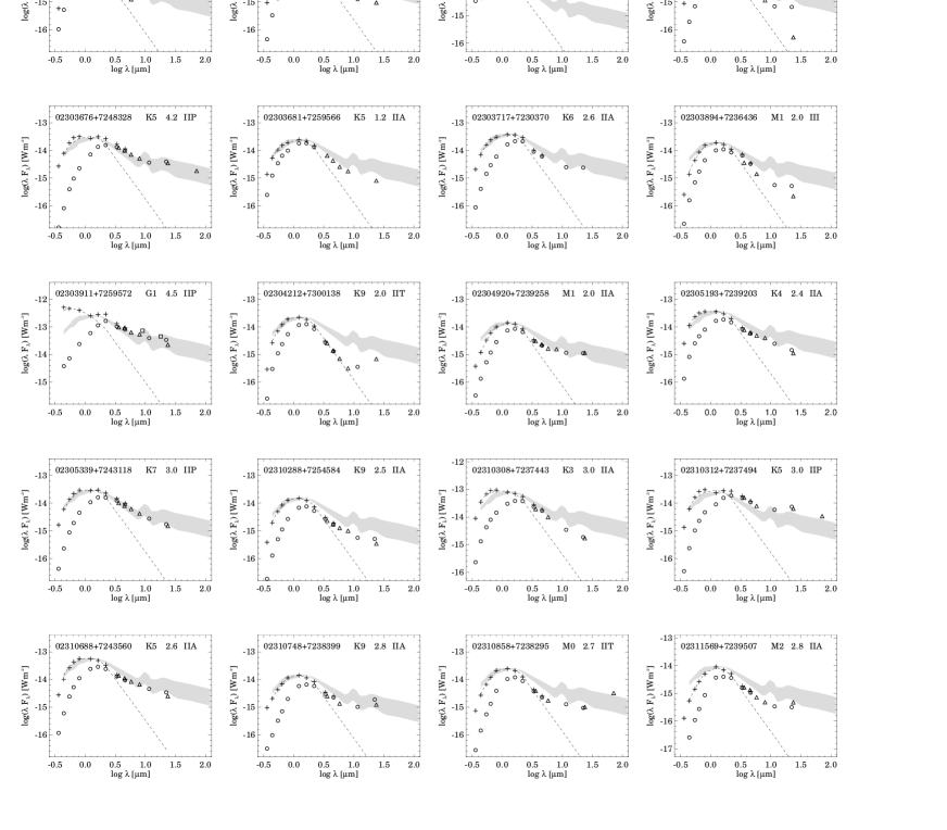
Figure 9: SEDs of the H$\alpha$ emission stars (continued.)

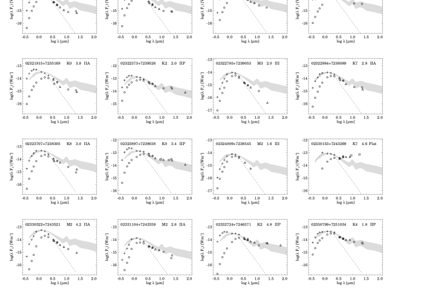
Figure 9: SEDs of the H$\alpha$ emission stars (continued.)

SEDs of the H$\alpha$ emission stars are shown in Fig. 9. The dereddened SED and that of the best fitting photosphere are also plotted. The photometry-based spectral type and extinction, as well as the SED slope type are indicated in each plot. According to the classification scheme (Lada, 1991; Greene et al., 1994), our list of H$\alpha$ emission stars contains one Class I source, 5 Flat SED, 64 Class II, and 5 Class III sources. Twenty-three of the Class II stars have primordial circumstellar disks (II P), 32 ones are surrounded by anemic disks (II A), and 9 pre-transitional / transitional disks (II T) can be found in the sample.

4.4.2 Hertzsprung–Russell Diagram

Figure 10 shows the distribution of the H$\alpha$ emission stars in the HRD. Filled circles indicate the stars with spectral types determined from spectroscopic observations, and open circles show the stars whose spectral types were derived from photometric data. The diagram suggests that most of our selected candidate YSOs are pre-main sequence stars between ages of 1–3 million years, in the mass interval of 0.25–2.0 M_☉, adopting a distance of 825 pc. Part of the stars are apparently older, and there are a few objects near or even below the ZAMS. The H$\alpha$ star below the ZAMS is 2MASS 02275976+7235561, aka HH 488 S. This object is a binary or multiple system (Kumar et al., 2003), exhibiting a Flat SED (Fig. 9). Another underluminous star, apparently located on the ZAMS, is the central star of RNO 8, mentioned in Sect. 4.3.2. These stars may have nearly edge-on disks, blocking most of the optical photospheric fluxes. Combination of random uncertainties in photometry, spectral type, extinction, and veiling may also result in uncertain values of luminosity and temperature (see Manara et al., 2013). We used Siess et al.’s (2000) pre-main sequence evolutionary models to estimate the masses of the H$\alpha$ emission stars and their uncertainties. We did not attempt to deduce age distribution from the luminosity distribution. Spectral types, visual extinctions, $T_{\mathrm{eff}}$, $L$ /$L_{\sun}$, and the SED slope types of the H$\alpha$ emission stars are listed in Table 6.

4.4.3 Accretion Rates

The major source of the H$\alpha$ emission of pre-main sequence stars is gas falling onto the stellar surface along magnetospheric accretion columns. Several empirical relationships have been established between the luminosity of the H$\alpha$ line and accretion luminosity (e.g. Dahm, 2008; Herczeg & Hillenbrand, 2008; Fang et al., 2009; Barentsen et al., 2011). We computed accretion rates for our H$\alpha$ emission stars using the relationship established by Barentsen et al. (2011) for the H$\alpha$ emission stars of IC 1396, spreading nearly on the same mass interval as our stars:

$$\log(L_{\mathrm{acc}}/L_{\sun})=(1.13\pm 0.07)\log(L_{\hbox{H$\alpha$}}/L_{\sun})+(1.93\pm 0.23)$$ (1)

where $L_{\hbox{H$\alpha$}}$ is the luminosity of the H$\alpha$ emission line. To convert the luminosity $L_{\mathrm{acc}}$ to accretion rate $\dot{M}_{\mathrm{acc}}$, according to the relationship

$$L_{\mathrm{acc}}\approx\frac{G\dot{M}_{acc}M_{*}}{R_{*}}\left(1-\frac{R_{*}}{R_{0}}\right),$$

we took the stellar mass $M_{*}$, and radius $R_{*}$ from the HRD, and adopted $R_{0}\approx 5\,R_{*}$ for the inner radius of the gaseous disk (Gullbring et al., 1998). Logarithms of the resulting $\dot{M}_{\mathrm{acc}}$ accretion rates are listed in the eighth column of Table 6, and $\dot{M}_{\mathrm{acc}}$ is plotted against the stellar mass $M_{*}$ in Fig. 11. Stars of different SED shapes are distinguished. Filled circle indicates the only Class I H$\alpha$ star, and open circles mark the Flat SED sources. Squares show the II P type SEDs. Upward triangles are for II A type SEDs, and downward triangles mark the II T type SEDs. Class III sources are plotted with diamonds. Similarly to several other young stellar groups (e.g Natta et al., 2006; Herczeg & Hillenbrand, 2008; Barentsen et al., 2011), a trend can be seen in the widely scattered points. The linear fit to the data,

$$\log\dot{M}=(1.49\pm 0.36)\log M-(7.87\pm 0.09),$$

is shown by the solid line. Its slope is consistent with the values between 1.0 and 3.0, found for other star-forming regions (e.g Natta et al., 2006; Herczeg & Hillenbrand, 2008; Barentsen et al., 2011). The median $\dot{M}_{\mathrm{acc}}$ of the sample is $7.6\times 10^{-9}$ M_☉ yr^-1, a typical value for T Tauri stars. Taking into account the 10% uncertainty of EW(H$\alpha$) and the errors listed in Table 6 we find that the accretion rates are accurate within $\approx 0.3--0.5$ order of magnitude. Using another empirical relationship results in slightly higher accretion luminosities, but does not affect the shape of the $\dot{M}_{\mathrm{acc}}$ vs. $M_{\mathrm{star}}$ plot.

The U-band magnitudes, available for the H$\alpha$ emission stars, may offer an independent way to derive accretion rates. Since most of our stars are faint in the U-band, and their spectral types, determined from non-simultaneous photometric data, can be regarded as preliminary estimates, we calculated the accretion rates for a carefully subsample. First we selected stars with U$<21.0$ mag and $\delta U<0.1$. Then we inspected the SEDs of the pre-selected stars and omitted those whose SED indicated photometric variation between the I-band (obtained in 2005) and J-band (1999) fluxes, adding to the uncertainties of the derived spectral type and extinction. For the fifteen remaining stars (Nos. 1, 7, 9, 16, 18, 20, 28, 29, 32, 41, 43, 46, 47, 65, 66) we computed the U-band excess luminosities and transformed them into accretion luminosities following the procedures described by Gullbring et al. (1998). Photospheric U-band luminosities were adopted from Kenyon & Hartmann (1995). Comparing the result with the H$\alpha$ luminosities we obtain the relation

$$\log(L_{\mathrm{acc}}/L_{\sun})=(1.18\pm 0.11)\log(L_{\hbox{H$\alpha$}}/L_{\sun})+(1.65\pm 0.22),$$

compatible with Eq. 1. Figure 12 shows the relation between $\log L_{\hbox{H$\alpha$}}$ and $\log L_{\mathrm{U_{exc}}}$. The estimated uncertainities are within an order of magnitude.

5 DISCUSSION

5.1 New Features of the Cloud Structure

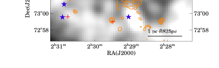
Figure 13: Extinction map of the central $\sim 18\times 11$ arcmin area of the clump L1340 B, with the 850 $\mu$m contours (orange) overplotted. Blue asterisks indicate the stars associated with the reflection nebula DG 9, and red plusses show the IRAS point sources.

The new extinction map of L1340 reveals a shallow, strongly fragmented cloud. The average hydrogen column density within the $A_{\mathrm{V}}=1$ mag contour is $N(H_{2})\approx 1.87\times 10^{21}$ cm^-2. If they exist, high column density regions, a prerequisite of star formation, are smaller in diameter than some 0.35 pc, the resolution of our map. The 850 $\mu$m map of L1340 B (Di Francesco et al., 2008) and the NH₃ cores (Paper II) point to such regions. The average hydrogen column densities, obtained from $A_{\mathrm{V}}$ for the clumps L1340 A, B, and C, are around $N(H_{2})\lesssim 2.5\times 10^{21}$ cm^-2 (Table 5), lower than the detection threshold for C¹⁸O (e.g. Pineda et al., 2008), suggesting that C¹⁸O was detected from dense, small regions of a knotty formation. The past and present winds and outflows of embedded intermediate-mass stars have probably played a role in sustaining the knotty structure, as it has been discussed by Offner & Arce (2015). This effect is demonstrated by Fig. 13, in which the extinction map of the central part of the clump L1340 B, containing the stars illuminating the DG 9 nebula is displayed, together with the 850-µm contours. The figure reveals several small, bubble-like features in the extinction, the most conspicuous one around the A0-type star 02290319+7259366 (star I5 in Fig. 1), bordered by dark lanes or submillimeter emission and embedded protostellar sources.

5.2 The Optically Selected YSO Population of L1340

The pre-main sequence evolutionary time of the most massive star associated with L1340 is a few times $10^{5}$ years (Palla & Stahler, 1993; Siess et al., 2000). In spite of the absence of conspiuous pre-main sequence features this star may be very young, similar in several respects to BD$+65^{o}1638$ in the young cluster NGC 7129 (Dahm & Hillenbrand, 2015). The temporary, weak emission component, detected in its H$\alpha$ line, supports this argument. The weak emission components, suspected in the H$\alpha$ lines of other intermediate-mass stars, have to be confirmed by high-resolution spectroscopic observations.

Our sample of candidate T Tauri stars contains 5 G-type, 50 K-type, and 21 M-type stars. The median mass of the H$\alpha$ emission population is 0.7 M_☉. A sizeable part of the young population of the cloud is expected below the detection threshold of the slitless spectroscopic observations. The lower mass limit is 0.25 M_☉ corresponding to a spectral type of $\sim$ M3. The cumulative distribution of the derived stellar masses is shown in Fig. 14. The slope of the line, fitted to the data over the $0.3\leq M_{*}/M_{\sun}\leq 3.0$ region,

$$\log N(M_{*}>m)=(-1.38\pm 0.09)\log m+(1.44\pm 0.025)$$

is compatible with that of Salpeter’s (1955) initial mass function.

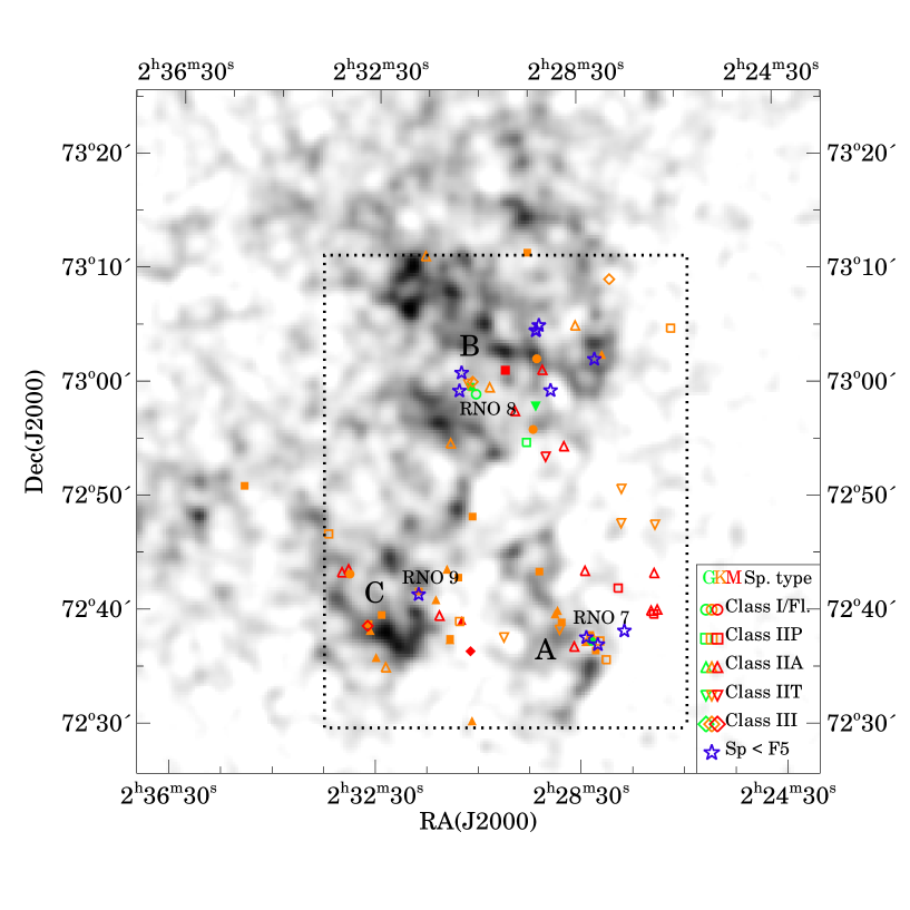
Figure 15: Distribution of the intermediate-mass stars earlier than F5 type (blue star symbols) and H$\alpha$ emission stars, overplotted on the extinction map of the region. Dotted lines outline the area of the WFGS2 survey. The lowest contour is drawn at $A_{\mathrm{V}}=1.5$ mag, and the increment is 1 mag. Filled symbols indicate stars with $\dot{M}_{\mathrm{acc}}\geq 7.6\times 10^{-9}$ M_☉ yr^-1, and stars plotted with open symbols accrete slower than the median of the sample.

The surface distribution of the candidate young stellar population, overplotted on the extinction map of the cloud, is displayed in Fig. 15. G, K, and M-type T Tauri star candidates are plotted with different colors, and the SED classes are distinguished by the plotting symbol. Filled symbols indicate stars with accretion rates higher than the median $7.6\times 10^{-9}$ M_☉ yr^-1, while open symbols show the stars accreting more slowly than the median. Figure 15 shows that the H$\alpha$ emission stars are scattered over the observed area. [KOS94] HA 4 and [KOS94] HA 13 are projected outside of the area covered by the WFGS2 observatons, suggesting a possible more widely extended pre-main sequence star population.

A striking group is the cluster RNO 7, projected within the clump L1340 A, and containing 14 H$\alpha$ emission stars. Further small groups, consisting of less than ten members can be seen over the observed area. The most massive stars, including four of the five G-type T Tauri stars, are associated with the most massive cloud clump L1340 B. ¹³CO and NH₃ observations (Paper I, Paper II) have shown that the kinetic temperature of the molecular gas is higher in clump B than in clumps A and C. The stars projected on L1340 B, however, form a widely scattered aggregate, without conspicuous clustering, unlike other star-forming regions, exhibiting stronger clustering around more massive young stars (e.g. Testi et al., 1999; Lundquist et al., 2014).

Figure 15 shows clearly that K-type stars dominate our H$\alpha$ emission sample. It suggests also that II T type disks tend to be projected on low-extinction regions. Within the wide scatter of the points in Fig. 11 it can be noticed that none of the downward triangles (pre/transitional disks) are found above the fitted line, indicating that their accretion rates are lower than the average. To examine in more detail how the shape of the SED of a H$\alpha$ emission star is related to stellar properties, accretion activity, and location within the cloud, we show in Table 7 the average EW(H$\alpha$), $A_{\mathrm{V}}$, $\log T_{\mathrm{eff}}$, $\log L$, and $\dot{M}_{\mathrm{acc}}$ for each SED class and subclass. The comparison shows that Flat and Class II P sources are located in regions of higher extinction, they are more massive and their accretion rates are higher than those of the stars possessing II A and II T type disks. Similar correlations of the SED shapes with accretion rates and stellar distributions were reported for the Taurus Class II stars by Najita et al. (2007) and Luhman et al. (2010), respectively. It is noteworthy that the transitional disks of our sample (stars 7, 50), exhibiting photospheric SED below 24 µm, and weak/pre-transitional disks without excess emission below 8 µm  (stars 3, 4, 6) were identified as H$\alpha$ emission stars, suggesting CTTS-like accretion rates.

The age range of our target stars can be poorly constrained without further spectroscopic data. The HRD positions suggest that it may be comparable with that of the Taurus pre-main sequence population (cf. fig. 7 of Luhman et al., 2009). The number of Class II YSOs are also similar in both star-forming regions (Luhman et al., 2010; Kun et al., 2016), whereas they are different in volume, molecular mass and kinetic temperature, structure, and Galactic environment (Kenyon, Gómez, & Whitney, 2008). To check whether disk properties observed in the two apparently coeval star-forming regions can be distinguished or not, we collected statistical data in Table THE INTERMEDIATE-MASS STAR FORMING REGION LYNDS 1340. AN OPTICAL VIEW. We keep in mind that L1340 is some six times as distant as Taurus, therefore the low-mass side of its mass spectrum is more incompletely sampled. Furthermore, the H$\alpha$ emission stars are more massive and stronger accretors than the Class II average of the region. Table THE INTERMEDIATE-MASS STAR FORMING REGION LYNDS 1340. AN OPTICAL VIEW suggests that the Class II disks of L1340 and Taurus cannot be distinguished based on Spitzer color indices and mean accretion rates.

5.3 Comparison with Other IM SFRs

Lundquist et al. (2014, 2015) identified and studied a large sample of Galactic IM SFRs. Most of them are located significantly farther from us than L1340 and typically contain loose clusters with less than 100 members. The mean gas column densities and ¹³CO linewidths observed for L1340 are within the range found for this sample. The sample of 36 young clusters within our 1-kpc environment, studied by Gutermuth et al. (2009), contains several young stellar groups whose most massive star is around 5–6 M_☉ (e.g. IC 348, IRAS 20050+2720, BD$+40^{\mathrm{o}}4124$, NGC 7129). Unlike L1340, most of these star-forming regions are parts of giant molecular cloud complexes. L1340 is located at some 160 pc above the Galactic plane, near the outermost boundary of the molecular gas disk, far from any known giant molecular cloud. In this respect it is similar to NGC 7129, lying at a similar distance from the Galactic plane. Molecular clouds and star formation at intermediate Galactic latitudes may be produced by expanding superbubbles. No such object has been identified in the environment of L1340. Infalling high velocity clouds, or Kelvin–Helmholtz instabilities arising at the shearing surface between gas layers of different velocities may also compress the gas. Detailed examination of the velocity fields of the apparent swirling structures, seen in the WSSA (Meisner & Finkbeiner, 2014) image of the large-scale environment of L1340 may shed light on the interstellar processes leading to star formation in L1340.

6 CONCLUSIONS

We studied the structure and optically selected young stellar population of the molecular cloud L1340, located within our 1-kpc environment, but poorly studied so far. Our optical spectroscopic and photometric search for young stellar objects associated with the molecular cloud L1340 revealed that the most massive star associated with this cloud is a B4 type, 5 M_☉ star. The new spectroscopic and photometric data of the intermediate mass members led to a distance of $825^{+110}_{-80}$ pc, and revealed 14 candidate members of the young stellar population with $M\gtrsim 2$ M_☉. Our search for H$\alpha$ emission line stars, conducted with the WFGS2 instrument on the $2.2$-meter telescope of the University of Hawaii and covering a $30\arcmin\times 40\arcmin$ area, resulted in the detection of 75 candidate low-mass pre-main sequence stars, 58 of which are new. We constructed SEDs of our target stars, based on SDSS, 2MASS, Spitzer, and WISE photometric data, derived their spectral types, extinctions, and luminosities from BVRIJ fluxes, estimated masses by means of pre-main sequence evolutionary models, and examined the disk shapes utilizing the 2–24 µm interval of the SED. We measured the equivalent width of the H$\alpha$ line and derived accretion rates. The new extinction map of L1340, based on SDSS data, suggests a shallow cloud of clumpy structure, having a mass of some 3700 M_☉. The optically selected sample of pre-main sequence stars has a median effective temperature of 3970 K, stellar mass 0.7 M_☉, and accretion rate of 7.6$\times 10^{-9}$ M_☉ yr^-1. The highest mass stars and the highest extinction are associated with the largest clump of the cloud. However, the surface distribution of the young stars is more scattered in the largest clump than in the smaller ones.

Appendix A PHOTOMETRIC DATA OF THE OPTICALLY SELECTED CANDIDATE PMS STARS

We list UBVR_CI_C and 2MASS JHK_s magnitudes of the optically selected candidate young stars associated with L1340 in Table A1. Table A2 contains the Spitzer [3.6], [4.5], [5.8], [8.0], [24], and [70.0] magnitudes, and AllWISE [3.4], [4.6], [12], and [22] magnitudes for the same stars.

 

Figure 5: Spectra of [KOS94] HA stars and nebulous stars associated with RNO 7, RNO 8 and RNO 9. Insets show a zoom on the H$\alpha$ lines.

Figure 7: SEDs of the stars earlier than F5 and associated with optical or infrared nebulosities. Open circles show the SDSS, 2MASS, and WISE data, and triangles result from our Spitzer photometry. Plusses indicate the dereddened SED, and the dashed line shows the photospheric SED of the spectral type, derived from our spectroscopic data, matched to the extinction-corrected $I_{\mathrm{C}}$ band flux. 2MASS identifiers, spectral types and derived $A_{\mathrm{V}}$ extinctions are given at the top of each panel.

Figure 11: Accretion rates, derived from the H$\alpha$ luminosites as a function of the stellar mass. The filled circle is the only Class I source, open circles indicate the Flat SED sources. II P type SEDs are marked by squares. Upward triangles show II A sources, downward triangles are for II T type SEDs, and diamonds show the Class III young stars. The linear fit to the data is also drawn.

Figure 12: Logarithms of U-band excess luminosities of fifteen selected H$\alpha$ emission stars, plotted against the logarithms of H$\alpha$ luminosities.

Figure 14: Cumulative mass distribution of the candidate young stars identified during the present work, derived from their positions in the HRD, using the pre-main sequence evolutionary models of Siess et al. (2000). Solid line shows the linear fit to the data between 0.5 and 3 M_☉.

Table 1: Log of spectroscopic observations

No.	2MASS Id	Other id.	Date of obs.	$\lambda\lambda$ (Å)	Tel./Instr.
Candidate Intermediate-mass Young Stars
I1	02273807+7238267	$\cdots$	2011.09.27	3800–7500	Konkoly RCC
I2	02280942+7237162	$\cdots$	2004.12.08	3800–7500	FLWO 1.5-m/FAST
I3	02281033+7302197	$[KOS94]$ R1	2004.10.31	3800–7500	FLWO 1.5-m/FAST
I4	02282291+7237539	$\cdots$	2004.11.06	3800–7500	FLWO 1.5-m/FAST
I5	02290319+7259366	$[KOS94]$ R2	1999.11.05	3800–7500	FLWO 1.5-m/FAST
I6	02291684+7305197	$[KOS94]$ R3	1999.08.07	4900–7800	CA 2.2-m/CAFOS/G-100
I6	02291684+7305197	$[KOS94]$ R3	2004.11.06	3800–7500	FLWO 1.5-m/FAST
I7	02292000+7304545	$[KOS94]$ R3-2A	2004.11.05	3800–7500	FLWO 1.5-m/FAST
I8	02292062+7304514	$[KOS94]$ R3-2B	2004.11.05	3800–7500	FLWO 1.5-m/FAST
I9	02304997+7301100	$[KOS94]$ R4	2005.09.13	4900–7800	CA 2.2-m/CAFOS/G-100
I10	02305176+7259481	$\cdots$	2004.12.08	3800–7500	FLWO 1.5-m/FAST
I11	02314031+7241419	RNO 9	1999.08.07	4900–7800	CA 2.2-m/CAFOS/G-100
I11	02314031+7241419	RNO 9	2004.12.11	3800–7500	FLWO 1.5-m/FAST
Candidate Low-mass Pre-Main Sequence Stars
T1	02281661+7237328	$[KOS94]$ HA 1	1999.08.07	4900–7800	CA 2.2-m/CAFOS/G-100
T2	02281782+7238009	$[KOS94]$ HA 2	1999.08.07	4900–7800	CA 2.2-m/CAFOS/G-100
T3	02285180+7239143	$[KOS94]$ HA 5	1999.08.07	4900–7800	CA 2.2-m/CAFOS/G-100
T4	02292109+7258120	$[KOS94]$ HA 9	1999.08.07	4900–7800	CA 2.2-m/CAFOS/G-100
T5	02293037+7311429	$[KOS94]$ HA 4	1999.08.07	4900–7800	CA 2.2-m/CAFOS/G-100
T6	02303247+7259177	IRAS 02259+7246	2000.01.05	5825–8350	NOT/ALFOSC/Grism 8
T7	02303681+7259566	RNO 8 West	2000.01.05	5825–8350	NOT/ALFOSC/Grism 8
T8	02303911+7259572	RNO 8 East	2000.01.05	5825–8350	NOT/ALFOSC/Grism 8
T9	02313994+7241575	RNO 9 B	2005.09.13	4900–7800	CA 2.2-m/CAFOS/G-100
T10	02323897+7239038	$[KOS94]$ HA 10	2004.12.10	3800–7500	FLWO 1.5-m/FAST
T10	02323897+7239038	$[KOS94]$ HA 10	2004.12.10	3800–7500	FLWO 1.5-m/FAST
T10	02323897+7239038	$[KOS94]$ HA 10	1999.08.07	4900–7800	CA 2.2-m/CAFOS/G-100
T10	02323897+7239038	$[KOS94]$ HA 10	2004.12.10	3800–7500	FLWO 1.5-m/FAST
T11	02330153+7243269	$[KOS94]$ HA 11	2003.02.05	4900–7800	CA 2.2-m/CAFOS/G-100
T12	02350799+7251034	$[KOS94]$ HA 13	1999.08.07	4900–7800	CA 2.2-m/CAFOS/G-100
T12	02350799+7251034	$[KOS94]$ HA 13	2004.12.10	3800–7500	FLWO 1.5-m/FAST

Table 2: Coordinates, H$\alpha$ equivalent widths, and cross-identifiers of the H$\alpha$ emission stars

N	2MASS /SDSS Id.	EW(H$\alpha)$(Å)	Other Id./Associated object
1	02263797+7304575	84.7$\pm$4.5
2	02265909+7240166	16.7$\pm$2.0
3	02270033+7247439	41.3$\pm$1.3
4	02270211+7243289	15.2$\pm$7.4
5	02270324+7239529	240.0$\pm$80.0
6	02270625+7240113	25.05$\pm$16.8
7	02273962+7250548	16.7$\pm$1.1
8	02274044+7247536	24.0$\pm$0.8
9	02274486+7242119	37.6$\pm$4.9
10	02275138+7309197	14.0$\pm$2.5
11	02275976+7235561	280.0$\pm$60.0	HH 488S
12	02280135+7302439	171.9$\pm$28.7
13	02280700+7237345	49.0$\pm$5.0	RNO7-2
14	02281182+7236447	49.4$\pm$4.0	RNO7-3
15	02281259+7237067	$\cdots$	RNO7-4
16	02281661+7237328	18.5$\pm$0.9	IRAS 02236+7224, [KOS94]HA 1, RNO7-5, T1
17	02281748+7237384	60.5$\pm$5.0	RNO7-6
18	02281782+7238009	42.0$\pm$4.2	[KOS94]HA 2, RNO7-7, T2
19	02281808+7237437	37.5$\pm$6.0	RNO7-8
20	02281818+7238069	23.6$\pm$2.7	RNO7-9
21	02281877+7238091	$\cdots$	RNO7-10
22	02282357+7237317	29.7$\pm$2.4	RNO7-11
23	02282383+7243450	26.2$\pm$2.0
24	02283311+7305182	26.9$\pm$4.0
25	02283719+7237061	9.6$\pm$6.8	RNO7-12
26	02284780+7254422	42.8$\pm$35.2
27	02285180+7239143	84.0$\pm$4.6	[KOS94] HA 5, T3
28	02285420+7238352	68.1$\pm$17.3	RNO7-14
29	02285635+7240171	83.1$\pm$11.8
30	022856.42+724019.2	53.0$\pm$10.5
31	02285939+7239593	67.4$\pm$7.5
32	02290968+7253475	21.5$\pm$1.7
33	02291304+7301253	14.8$\pm$2.5
34	02291769+7243426	64.4$\pm$4.9
35	02291961+7302237	51.3$\pm$5.0
36	02292109+7258120	17.8$\pm$0.8	[KOS94] HA 9, T4
37	02292440+7256114	57.9$\pm$20.8
38	022932.28+725503.2	72.0$\pm$10.0
39	02294589+7257489	15.5$\pm$8.0
40	02295744+7301240	101.6$\pm$17.6
41	02295974+7237566	44.4$\pm$5.4
42	02301621+7259542	18.9$\pm$4.3
43	02303247+7259177	39.4$\pm$2.6	IRAS 02249+7230, RNO 8, T6
44	02303659+7300233	43.9$\pm$4.9
45	02303676+7248328	85.2$\pm$13.0
46	02303681+7259566	60.8$\pm$6.0	RNO8W, T7
47	02303717+7230370	41.7$\pm$4.8
48	02303894+7236436	185.7$\pm$81.9
49	02303911+7259572	29.1$\pm$1.7	RNO8E, T8
50	02304212+7300138	33.7$\pm$5.9
51	02304920+7239258	93.02$\pm$9.0
52	02305193+7239203	30.1$\pm$4.3
53	02305339+7243118	70.9$\pm$20.9
54	02310288+7254584	15.0$\pm$5.0
55	02310308+7237443	108.7$\pm$16.4
56	02310312+7237494	69.2$\pm$7.0
57	02310688+7243560	64.6$\pm$4.5
58	02310748+7238399	$\cdots$
59	02310858+7238295	$\cdots$
60	02311569+7239507	166.1$\pm$41.5
61	02311975+7241146	36.6$\pm$5.5
62	02313341+7311247	36.14$\pm$21.7
63	02313994+7241575	33.7$\pm$6.0	RNO9 B, T9
64	02321260+7230136	$\cdots$
65	02321815+7235169	30.8$\pm$3.7
66	02322373+7239526	7.8$\pm$0.6
67	02322785+7239053	31.0$\pm$5.0
68	02322984+7236089	76.5$\pm$23.8
69	02323707+7238305	17.49$\pm$13.0
70	02323897+7239038	57.8$\pm$6.0	IRAS F02279+7225, [KOS94] HA 10, T10
71	02324009+7238545	147.0$\pm$14.0
72	02330153+7243269	496.0$\pm$110.0	IRAS 02283+7230, [KOS94] HA 11, V1180 Cas, T11
73	02330322+7243521	22.10$\pm$6.1
74	02331104+7243359	34.2$\pm$6.0
75	02332724+7246571	30.48$\pm$5.63

Table 3: Results for the B, A, F type stars associated with L1340

No.	2MASS Id	Sp. type	$A_{\mathrm{V}}$	$T_{\mathrm{eff}}$	$L_{\mathrm{star}}$	Mass	HRD
			(mag)	(K)	(L☉)	(M☉)
I1	02273807+7238267	A0	0.5	$9700^{+700}_{-500}$	$50.6^{+15.8}_{-12.0}$	2.5	PMS
I2	02280942+7237162	F2	0.5	$6810^{+0220}_{-90}$	$4.4^{+1.4}_{-1.0}$	1.5	ZAMS
I3	02281033+7302197	B5	0.9	$15700^{+1000}_{-1200}$	$512.0^{+159.6}_{-121.7}$	5.0	ZAMS
I4	02282291+7237539	A5	1.2	$8080^{+190}_{-80}$	$13.1^{+4.1}_{-3.1}$	2.0	ZAMS
I5	02290319+7259366	A0	1.3	$9700^{+700}_{-500}$	$56.0^{+17.5}_{-13.3}$	2.5	PMS
I6	02291684+7305197	B4	1.4	$16700^{+300}_{-1000}$	$649.0^{+202.3}_{-154.3}$	5.0	ZAMS
I7	02292000+7304545	A3	0.9	$8550^{+290}_{-280}$	$20.5^{+6.4}_{-4.9}$	2.0	ZAMS
I8	02292062+7304514	A5	1.0	$8080^{+190}_{-80}$	$12.1^{+3.8}_{-2.9}$	2.0	ZAMS
I9	02304997+7301100	A2	1.2	$8840^{+360}_{-80}$	$68.2^{+21.3}_{-16.2}$	2.5	PMS
I10	02305176+7259481	B8	2.7	$6640^{+80}_{-130}$	$248.3^{+77.4}_{-59.0}$	3.5	PMS
I11	02314031+7241419	F4	3.5	$12500^{+1500}_{-1800}$	$21.3^{+6.6}_{-5.1}$	2.0	PMS

Table 4: Spectral types and H$\alpha$ equivalent widths of the T Tauri type targets of our longslit observations.

No.	2MASS Id	Sp. Type	EW(H$\alpha$)	EW(H$\alpha$)(WFGS2)
T1	02281661+7237328	G2	$26.4\pm 0.8$	$18.5\pm 0.9$
T2	02281782+7238009	K4	$43.2\pm 0.7$	$42.0\pm 4.2$
T3	02285180+7239143	K4	$109.0\pm 11.0$	$84.0\pm 4.6$
T4	02292109+7258120	G4	$20.5\pm 1.5$	$17.8\pm 0.8$
T5	02293037+7311429	K6	$76.0\pm 10.0$	$\cdots$
T6	02303247+7259177	G7	$33.6\pm 1.5$	$39.4\pm 2.6$
T7	02303681+7259566	K5	$62.6\pm 2.0$	$60.8\pm 6.0$
T8	02303911+7259572	G1	$20.3\pm 1.2$	$29.1\pm 1.7$
T9	02313994+7241575	K5	$16.2\pm 0.6$	$33.7\pm 6.0$
T10	02323897+7239038	K0	$55.9\pm 2.0$	$57.8\pm 6.0$
T10	02323897+7239038	K0	$45.0\pm 1.2$
T11	02330153+7243269	K7	$300.0\pm 15.0$	$496.0\pm 110$
T12	02350799+7251034	K4	$125.5\pm 12.0$	$115.9\pm 7.3$
T12	02350799+7251034	K4	$109.0\pm 5.0$	$\cdots$

Table 5: Properties of the major clumps of L1340

Clump	Size	$\langle A_{\mathrm{V}}\rangle$	$A_{\mathrm{V}}$(max)	Mass
	(pc)	(mag)	(mag)	(M☉)
A	1.9	2.5	$>6.7$	185
B	5.0	2.6	$>6.7$	1325
C	3.4	2.6	$>6.7$	620

Table 6: Properties of the H$\alpha$ emission stars derived from the photometric and EW(H$\alpha$) data

No.	2MASS /SDSS	Sp.type	AV	Teff	Lstar	M∗	$\log\dot{M}_{\mathrm{acc}}$	SED Class
			(mag)	(K)	($L_{\sun}$)	($M_{\sun}$)
1	02263797+7304575	K4	0.7	$4330^{+430}_{-310}$	$0.35^{+0.25}_{-0.14}$	$1.10^{+0.20}_{-0.30}$	$-$8.5	II P
2	02265909+7240166	M1	1.5	$3630^{+250}_{-270}$	$0.16^{+0.11}_{-0.06}$	$0.40^{+0.10}_{-0.10}$	$-$9.6	II A
3	02270033+7247439	K3	1.3	$4550^{+370}_{-410}$	$0.86^{+0.61}_{-0.36}$	$1.25^{+0.20}_{-0.20}$	$-$8.2	II T
4	02270211+7243289	M0	2.2	$3770^{+170}_{-280}$	$0.38^{+0.27}_{-0.16}$	$0.55^{+0.05}_{-0.15}$	$-$9.1	II A
5	02270324+7239529	M0	2.2	$3770^{+250}_{-270}$	$0.13^{+0.09}_{-0.05}$	$0.40^{+0.10}_{-0.10}$	$-$8.4	II A
6	02270625+7240113	M0	1.8	$3770^{+170}_{-280}$	$0.30^{+0.21}_{-0.12}$	$0.55^{+0.05}_{-0.15}$	$-$8.9	II A
7	02273962+7250548	K3	1.2	$4550^{+370}_{-410}$	$0.99^{+0.70}_{-0.41}$	$1.20^{+0.20}_{-0.20}$	$-$8.6	II T
8	02274044+7247536	K4	1.4	$4330^{+430}_{-310}$	$1.32^{+0.93}_{-0.54}$	$1.00^{+0.15}_{-0.20}$	$-$8.3	II T
9	02274486+7242119	M0	1.2	$3770^{+170}_{-280}$	$0.28^{+0.20}_{-0.12}$	$0.55^{+0.05}_{-0.15}$	$-$8.8	II P
10	02275138+7309197	K9	1.2	$3940^{+80}_{-170}$	$0.12^{+0.08}_{-0.05}$	$0.60^{+0.10}_{-0.10}$	$-$10.0	III
11	02275976+7235561	K7	0.6	$3970^{+170}_{-90}$	$0.03^{+0.02}_{-0.01}$	$0.60^{+0.10}_{-0.10}$	$-$9.4	II P
12	02280135+7302439	K7	3.8	$3970^{+170}_{-90}$	$1.15^{+0.81}_{-0.48}$	$0.70^{+0.10}_{-0.10}$	$-$7.4	II A
13	02280700+7237345	K6	2.9	$4020^{+210}_{-80}$	$0.44^{+0.31}_{-0.18}$	$0.80^{+0.10}_{-0.10}$	$-$8.4	II P
14	02281182+7236447	K6	4.6	$4020^{+210}_{-80}$	$3.28^{+2.32}_{-1.36}$	$0.70^{+0.10}_{-0.10}$	$-$7.1	II P
15	02281259+7237067	M0	3.0	$3770^{+170}_{-280}$	$0.26^{+0.18}_{-0.11}$	$0.55^{+0.05}_{-0.15}$	$\cdots$	II A
16	02281661+7237328	G2	3.8	$5870^{+180}_{-250}$	$14.56^{+10.29}_{-6.03}$	$2.20^{+0.20}_{-0.20}$	$-$6.8	Flat
17	02281748+7237384	K4	4.0	$4330^{+430}_{-310}$	$1.09^{+0.77}_{-0.45}$	$1.10^{+0.10}_{-0.30}$	$-$8.0	II A
18	02281782+7238009	K1	3.8	$4920^{+250}_{-370}$	$5.27^{+3.73}_{-2.18}$	$2.10^{+0.40}_{-0.40}$	$-$7.4	Flat
19	02281808+7237437	K0	4.0	$5030^{+180}_{-270}$	$3.76^{+2.65}_{-1.55}$	$1.90^{+0.10}_{-0.20}$	$-$7.6	II P
20	02281818+7238069	K5	2.9	$4140^{+410}_{-170}$	$3.49^{+2.46}_{-1.44}$	$0.80^{+0.40}_{-0.15}$	$-$7.5	II P
21	02281877+7238091	K8	2.4	$3940^{+80}_{-170}$	$1.78^{+1.26}_{-0.74}$	$0.60^{+0.10}_{-0.10}$	$\cdots$	II A
22	02282357+7237317	K8	3.3	$3940^{+80}_{-170}$	$1.27^{+0.89}_{-0.52}$	$0.60^{+0.10}_{-0.10}$	$-$8.0	II A
23	02282383+7243450	M3	1.7	$3360^{+270}_{-480}$	$0.21^{+0.15}_{-0.09}$	$0.30^{+0.10}_{-0.15}$	$-$9.2	II A
24	02283311+7305182	K8	3.5	$3940^{+80}_{-170}$	$1.03^{+0.73}_{-0.43}$	$0.60^{+0.10}_{-0.10}$	$-$8.2	II A
25	02283719+7237061	M1	2.3	$3630^{+250}_{-270}$	$1.33^{+0.94}_{-0.55}$	$0.40^{+0.20}_{-0.10}$	$-$8.3	II A
26	02284780+7254422	M1	2.8	$3630^{+250}_{-270}$	$0.40^{+0.28}_{-0.16}$	$0.40^{+0.20}_{-0.10}$	$-$8.4	II A
27	02285180+7239143	K4	1.9	$4330^{+430}_{-310}$	$1.60^{+1.13}_{-0.66}$	$1.10^{+0.40}_{-0.30}$	$-$7.6	II P
28	02285420+7238352	K0	3.8	$5030^{+180}_{-270}$	$0.81^{+0.57}_{-0.34}$	$1.10^{+0.10}_{-0.10}$	$-$8.2	II T
29	02285635+7240171	K6	2.8	$4020^{+210}_{-80}$	$1.66^{+1.17}_{-0.69}$	$0.70^{+0.20}_{-0.10}$	$-$7.3	II A
30	022856.42+724019.2	$\cdots$	$\cdots$	$\cdots$	$\cdots$	$\cdots$	$\cdots$	$\cdots$
31	02285939+7239593	K3	3.2	$4550^{+370}_{-410}$	$2.93^{+2.07}_{-1.21}$	$1.50^{+0.30}_{-0.50}$	$-$7.3	II A
32	02290968+7253475	M0	1.4	$3770^{+170}_{-280}$	$0.87^{+0.62}_{-0.36}$	$0.55^{+0.10}_{-0.20}$	$-$8.3	II T
33	02291304+7301253	M2	1.6	$3490^{+180}_{-330}$	$0.15^{+0.11}_{-0.06}$	$0.35^{+0.05}_{-0.15}$	$-$9.6	II A
34	02291769+7243426	K7	1.7	$3970^{+170}_{-90}$	$1.39^{+0.98}_{-0.58}$	$0.65^{+0.05}_{-0.15}$	$-$7.5	II P
35	02291961+7302237	K5	6.5	$4140^{+410}_{-170}$	$1.85^{+1.30}_{-0.76}$	$0.80^{+0.30}_{-0.10}$	$-$7.6	Flat
36	02292109+7258120	G3	2.0	$5740^{+250}_{-230}$	$3.89^{+4.48}_{-2.63}$	$1.60^{+0.20}_{-0.20}$	$-$7.5	II T
37	02292440+7256114	K9	3.0	$3880^{+90}_{-250}$	$1.72^{+1.22}_{-0.71}$	$0.60^{+0.05}_{-0.20}$	$-$7.5	Flat
38	022932.32+725503.3	G8	3.0	$5210^{+170}_{-200}$	$\cdots$	$0.55^{+0.05}_{-0.15}$	$-$10.1	$\cdots$
39	02294589+7257489	M0	2.6	$3770^{+170}_{-280}$	$0.44^{+0.31}_{-0.18}$	$0.55^{+0.05}_{-0.15}$	$-$8.9	II A
40	02295744+7301240	M0	3.0	$3770^{+170}_{-280}$	$0.56^{+0.40}_{-0.23}$	$0.65^{+0.05}_{-0.15}$	$-$7.4	II P
41	02295974+7237566	K8	1.2	$3940^{+80}_{-170}$	$0.46^{+0.33}_{-0.19}$	$0.60^{+0.10}_{-0.20}$	$-$8.5	II T
42	02301621+7259542	K9	2.5	$3880^{+90}_{-250}$	$1.25^{+0.89}_{-0.52}$	$1.00^{+0.10}_{-0.10}$	$-$8.2	II A
43	02303247+7259177	G7	0.5	$5290^{+210}_{-170}$	$0.70^{+0.50}_{-0.29}$	$0.65^{+0.20}_{-0.10}$	$-$8.6	I
44	02303659+7300233	K7	2.6	$3970^{+170}_{-90}$	$0.64^{+0.45}_{-0.26}$	$0.80^{+0.30}_{-0.10}$	$-$8.3	III
45	02303676+7248328	K5	4.2	$4140^{+410}_{-170}$	$1.05^{+0.74}_{-0.43}$	$0.70^{+0.15}_{-0.10}$	$-$7.7	II P
46	02303681+7259566	K5	1.2	$4140^{+410}_{-170}$	$0.84^{+0.59}_{-0.35}$	$0.80^{+0.40}_{-0.10}$	$-$8.0	II A
47	02303717+7230370	K6	2.6	$4020^{+210}_{-80}$	$1.20^{+0.85}_{-0.50}$	$0.65^{+0.25}_{-0.05}$	$-$7.9	II A
48	02303894+7236436	M1	2.0	$3630^{+250}_{-270}$	$0.56^{+0.39}_{-0.23}$	$0.40^{+0.20}_{-0.10}$	$-$7.4	III
49	02303911+7259572	G1	4.5	$5970^{+120}_{-230}$	$13.93^{+9.84}_{-5.77}$	$2.00^{+0.20}_{-0.20}$	$-$7.3	II P
50	02304212+7300138	K9	2.0	$3880^{+90}_{-250}$	$0.67^{+0.47}_{-0.28}$	$0.60^{+0.10}_{-0.20}$	$-$8.4	II T
51	02304920+7239258	M1	2.0	$3630^{+250}_{-270}$	$0.38^{+0.27}_{-0.16}$	$0.40^{+0.20}_{-0.20}$	$-$8.0	II A
52	02305193+7239203	K4	2.4	$4330^{+430}_{-310}$	$1.29^{+0.91}_{-0.53}$	$1.10^{+0.30}_{-0.30}$	$-$8.1	II A
53	02305339+7243118	K7	3.0	$3970^{+170}_{-90}$	$0.99^{+0.70}_{-0.41}$	$0.80^{+0.15}_{-0.10}$	$-$7.8	II P
54	02310288+7254584	K9	2.5	$3880^{+90}_{-250}$	$0.46^{+0.32}_{-0.19}$	$0.60^{+0.10}_{-0.20}$	$-$9.0	II A
55	02310308+7237443	K3	3.0	$4550^{+370}_{-410}$	$3.21^{+2.27}_{-1.33}$	$1.50^{+0.50}_{-0.50}$	$-$7.0	II A
56	02310312+7237494	K5	3.0	$4140^{+410}_{-170}$	$0.96^{+0.68}_{-0.40}$	$0.60^{+0.10}_{-0.10}$	$-$7.8	II P
57	02310688+7243560	K5	2.6	$4140^{+410}_{-170}$	$1.99^{+1.40}_{-0.82}$	$0.80^{+0.30}_{-0.20}$	$-$7.4	II A
58	02310748+7238399	K9	2.8	$3880^{+90}_{-250}$	$0.42^{+0.29}_{-0.17}$	$0.60^{+0.10}_{-0.15}$	$\cdots$	II A
59	02310858+7238295	M0	2.7	$3770^{+170}_{-280}$	$0.74^{+0.53}_{-0.31}$	$0.55^{+0.05}_{-0.15}$	$\cdots$	II T
60	02311569+7239507	M2	2.8	$3490^{+180}_{-330}$	$0.22^{+0.15}_{-0.09}$	$0.35^{+0.05}_{-0.10}$	$-$8.2	II A
61	02311975+7241146	K8	2.6	$3940^{+80}_{-170}$	$0.84^{+0.59}_{-0.35}$	$0.60^{+0.04}_{-0.10}$	$-$8.2	II A
62	02313341+7311247	K3	2.6	$4550^{+370}_{-410}$	$1.06^{+0.75}_{-0.44}$	$1.30^{+0.15}_{-0.15}$	$-$8.3	II A
63	02313994+7241575	K5	3.5	$4140^{+410}_{-170}$	$1.24^{+0.88}_{-0.51}$	$0.80^{+0.40}_{-0.20}$	$-$8.0	II P
64	02321260+7230136	K2	3.5	$4760^{+270}_{-430}$	$0.96^{+0.68}_{-0.40}$	$1.20^{+0.30}_{-0.20}$	$\cdots$	II P
65	02321815+7235169	K0	3.8	$5030^{+180}_{-330}$	$1.57^{+1.11}_{-0.65}$	$1.50^{+0.30}_{-0.30}$	$-$8.2	II A
66	02322373+7239526	K4	2.0	$4330^{+370}_{-310}$	$2.89^{+4.00}_{-2.34}$	$1.50^{+0.30}_{-0.30}$	$-$7.6	II P
67	02322785+7239053	M3	2.0	$3360^{+270}_{-480}$	$0.25^{+0.18}_{-0.11}$	$0.30^{+0.10}_{-0.20}$	$\cdots$	III
68	02322984+7236089	K7	2.8	$3970^{+170}_{-90}$	$0.98^{+0.69}_{-0.41}$	$0.65^{+0.15}_{-0.05}$	$-$7.7	II A
69	02323707+7238305	K8	3.0	$3940^{+80}_{-170}$	$1.52^{+1.07}_{-0.63}$	$0.60^{+0.05}_{-0.10}$	$-$8.0	II A
70	02323897+7239038	K0	3.4	$5030^{+180}_{-270}$	$6.77^{+4.78}_{-2.80}$	$2.30^{+0.20}_{-0.20}$	$-$6.9	II P
71	02324009+7238545	M2	1.6	$3490^{+180}_{-330}$	$0.21^{+0.15}_{-0.09}$	$0.35^{+0.10}_{-0.12}$	$-$8.4	III
72	02330153+7243269	K7	4.6	$3970^{+170}_{-90}$	$3.19^{+2.25}_{-1.32}$	$0.65^{+0.15}_{-0.05}$	$-$5.8	Flat
73	02330322+7243521	M2	4.2	$3490^{+180}_{-330}$	$1.57^{+1.11}_{-0.65}$	$0.35^{+0.10}_{-0.10}$	$-$8.3	II A
74	02331104+7243359	M2	2.8	$3490^{+180}_{-330}$	$0.39^{+0.27}_{-0.16}$	$0.35^{+0.10}_{-0.10}$	$-$8.7	II A
75	02332724+7246571	K2	4.8	$4760^{+270}_{-430}$	$1.31^{+0.93}_{-0.54}$	$1.40^{+0.30}_{-0.20}$	$-$8.3	II P
76	02293037+7311429	K6	3.8	$4020^{+210}_{-80}$	$3.27^{+2.31}_{-1.35}$	$0.70^{+0.20}_{-0.05}$	$-$6.9	II P
77	02350799+7251034	K4	1.8	$4330^{+430}_{-310}$	$1.56^{+1.10}_{-0.65}$	$1.10^{+0.30}_{-0.30}$	$-$7.4	II P

Table 7: Distribution of SED slopes of the candidate PMS stars

SED Class	$\langle A_{\mathrm{V}}\rangle$	$\langle EW(\hbox{H$\alpha$})\rangle$	$\langle T_{\mathrm{eff}}\rangle$	$\langle M_{star}\rangle$	$\langle L_{star}\rangle$	$\langle\dot{M}_{\mathrm{acc}}\rangle$	N
	(mag)	(Å)	(K)	(M☉)	(L☉)	($10^{-9}$ M☉ yr-1)
I + Flat	3.80	135.0	4680	1.24	4.90	285.3	6
00II P	2.80	75.0	4340	1.00	2.28	31.9	23
00II T	1.84	33.4	4380	0.96	1.54	8.3	9
00II A	2.68	49.4	3910	0.68	1.00	15.5	32
II (P+T+A)	2.63	57.1	4140	0.83	1.98	21.7	64
III	1.88	14.0	3670	0.46	0.47	11.4	5

Table 8: Comparison of Class II YSOs in L1340 and Taurus

	L1340 H$\alpha$	L1340 Spitzer	Taurus Spitzer	Taurus ref.
Stars earlier than K6	26	37	23	1
K6 $\leq Sp.type<$ M3	38	71	90	1
M3 $\leq Sp.type<$ M6	2	44	44	1
Mean $K_{\mathrm{s}}-[5.8]$	1.52	1.29	1.38	1
Mean $K_{\mathrm{s}}-[8.0]$	2.24	1.94	2.20	1
Mean $K_{\mathrm{s}}-[24]$	4.96	4.78	5.16	1
Mean $\log\dot{M}_{acc}$	$-8.1$	$\cdots$	$-7.6$	2
00Primordial disks	$-7.6$	$\cdots$	$-7.6$	2
00Transitional disks	$-8.1$	$\cdots$	$-8.5$	2

References. — (1) Luhman et al. (2010); (2) Najita et al. (2007)

Table 9: Table A1. UBVR_CI_CJHK_s magnitudes of the optically selected candidate YSOs of L1340

N	U   dU	B   dB	V   dV	RC   dRC	IC   dIC	J   dJ	H   dH	Ks   dKs
Intermediate-mass stars
1	12.815 0.012	11.222 0.030	10.906 0.030	10.886 0.030	10.769 0.030	10.606 0.025	10.548 0.031	10.553 0.019
2	14.266 0.009	13.770 0.053	13.450 0.030	13.165 0.030	12.812 0.025	12.235 0.025	11.997 0.031	11.926 0.023
3	10.332 0.005	10.090 0.030	9.977 0.025	9.864 0.020	9.668 0.020	9.565 0.026	9.534 0.032	9.496 0.021
4	14.392 0.019	13.230 0.053	12.916 0.042	12.562 0.034	12.248 0.034	11.698 0.025	11.547 0.029	11.496 0.023
5	13.318 0.008	11.838 0.030	11.562 0.030	11.300 0.030	11.048 0.020	10.629 0.027	10.470 0.030	10.386 0.021
6	12.743 0.018	10.733 0.042	10.388 0.042	10.100 0.034	10.018 0.034	9.810 0.027	9.820 0.030	9.828 0.019
7	13.363 0.018	12.442 0.020	12.086 0.020	11.847 0.020	11.669 0.030	11.334 0.065	11.155 0.058	11.081 0.054
8	14.973 0.033	13.190 0.020	12.755 0.020	12.450 0.020	12.222 0.020	11.771 0.030	11.702 0.032	11.576 0.023
9	12.757 0.007	11.410 0.053	11.164 0.042	10.918 0.031	10.629 0.031	10.151 0.025	9.915 0.030	9.860 0.021
10	13.190 0.025	12.502 0.022	11.823 0.036	11.300 0.030	10.879 0.034	10.188 0.025	9.765 0.030	9.698 0.021
11	16.083 0.010	15.544 0.030	14.515 0.040	13.646 0.030	12.909 0.030	11.499 0.025	10.582 0.029	9.831 0.018
H$\alpha$ emission stars
1	16.810 0.014	16.509 0.006	15.648 0.006	15.084 0.007	14.316 0.007	14.211 0.031	13.403 0.037	13.034 0.028
2	22.784 1.007	21.276 0.030	19.646 0.030	18.415 0.018	16.796 0.014	15.167 0.044	14.428 0.046	14.152 0.052
3	19.056 0.045	17.949 0.007	16.489 0.007	15.598 0.007	14.783 0.008	13.578 0.026	12.875 0.028	12.630 0.022
4	23.127 1.610	20.862 0.021	19.156 0.021	17.870 0.014	16.204 0.011	14.581 0.034	13.661 0.041	13.309 0.033
5	22.645 0.283	22.006 0.046	20.235 0.046	18.982 0.026	17.453 0.021	15.645 0.054	14.718 0.062	14.328 0.069

Note. — Table A1 is published in its entirety in the electronic edition of the Astrophysical Journal. A portion is shown here for guidance regarding its form and content.

Table 10: Table A2. Spitzer and AllWISE magnitudes of the optically selected candidate YSOs of L1340

N	[3.6]  d[3.6]	[4.5]  d[4.5]	[5.8]  d[5.8]	[8.0]  d[8.0]	[24]  d[24]	[70]  d[70]	W1  dW1	W2  dW2	W3  dW3	W4  dW4
Intermediate-mass stars
1	10.600 0.034	10.624 0.034	10.662 0.033	10.697 0.037	$\cdots$	$\cdots$	10.378 0.023	10.393 0.020	8.903 0.036	7.208 0.101
2	11.944 0.040	11.912 0.034	11.990 0.059	11.976 0.032	$\cdots$	$\cdots$	11.751 0.023	11.720 0.021	$\geqq$11.750	$\geqq$9.228
3	9.506 0.034	9.525 0.040	9.559 0.036	9.606 0.038	$\cdots$	$\cdots$	9.431 0.023	9.451 0.020	9.574 0.051	$\geqq$8.933
4	11.493 0.034	11.487 0.035	11.503 0.037	11.525 0.037	$\cdots$	$\cdots$	11.436 0.023	11.394 0.022	11.041 0.131	$\geqq$8.838
5	10.358 0.033	10.352 0.033	10.387 0.034	10.455 0.038	$\cdots$	$\cdots$	10.337 0.023	10.299 0.021	9.519 0.128	8.740 0.362
6	9.834 0.034	9.830 0.033	9.832 0.035	9.817 0.034	8.984 0.082	$\cdots$	9.816 0.022	9.834 0.020	9.769 0.058	$\geqq$8.668
7	11.063 0.034	11.061 0.036	11.073 0.036	10.985 0.051	$\cdots$	$\cdots$	10.451 0.022	10.477 0.020	9.842 0.055	8.056 0.179
8	11.536 0.045	11.571 0.047	11.489 0.045	11.354 0.052	$\cdots$	$\cdots$	$\cdots$	$\cdots$	$\cdots$	$\cdots$
9	9.814 0.035	9.798 0.033	9.804 0.037	9.821 0.036	$\cdots$	$\cdots$	9.794 0.022	9.794 0.020	9.162 0.060	$\geqq$8.499
10	9.729 0.001	9.722 0.001	9.686 0.002	9.634 0.000	$\cdots$	$\cdots$	9.606 0.023	9.662 0.020	9.482 0.038	8.279 0.325
11	8.496 0.053	8.084 0.033	7.764 0.033	7.316 0.035	5.809 0.044	8.608 0.021	7.998 0.017	6.921 0.014	5.670 0.033	$\cdots$
H$\alpha$ emission stars
1	12.266 0.002	11.641 0.002	11.059 0.004	10.095 0.003	7.421 0.016	3.331 0.096	12.346 0.023	11.516 0.022	09.239 0.033	7.224 0.128
2	13.659 0.003	13.358 0.005	13.091 0.011	12.141 0.011	9.422 0.180	$\cdots$	13.734 0.024	13.331 0.026	11.527 0.173	$\geqq$8.498
3	12.596 0.002	12.428 0.003	12.160 0.006	11.193 0.005	7.260 0.015	$\cdots$	12.553 0.024	12.404 0.023	10.133 0.058	7.421 0.114
4	12.836 0.002	12.615 0.004	12.606 0.008	12.053 0.013	8.661 0.054	$\cdots$	13.041 0.025	12.719 0.026	11.724 0.199	$\geqq$8.241
5	13.449 0.003	12.960 0.004	12.902 0.010	11.827 0.009	8.780 0.088	$\cdots$	13.582 0.025	12.950 0.025	11.095 0.116	$\geqq$8.290

Note. — Table A2 is published in its entirety in the electronic edition of the Astrophysical Journal. A portion is shown here for guidance regarding its form and content.

References

- Ahn et al. (2012) Ahn, C. P., Alexandroff, R., Allende, P., et al. 2012, ApJS, 203, 21
- Allen et al. (2014) Allen, T. S., Prchlik, J. J., Megeath, S. T., et al. 2014, ApJ, 786, 113
- Arvidsson et al. (2010) Arvidsson, K., Kerton, C. R., Alexander, M. J., Kobulnicky, H. A., Uzpen, B. 2010, AJ, 140, 462
- Barentsen et al. (2011) Barentsen, G., Vink, J. S., Drew, J. E., et al. 2011, MNRAS, 415, 103
- Calvet et al. (2004) Calvet, N., Muzerolle, J., Briceño, C., et al. 2004, AJ, 128, 1294
- Cardelli et al. (1989) Cardelli, J. A., Clayton, G. C., & Mathis, J. S. 1989, ApJ, 345, 245
- Chavarría-K. (1981) Chavarría-K., C. 1981, A&A, 101, 105
- Cohen (1980) Cohen, M. 1980, AJ, 85, 29
- Cutri et al. (2003) Cutri, R. M., Skrutskie, M. F., van Dyk, S., et al. 2003, VizieR On-line Data Catalog: II/246
- Dahm (2008) Dahm, S. E. 2008, AJ, 136, 521
- Dahm & Hillenbrand (2015) Dahm, S. E., & Hillenbrand, L. A. 2015, AJ, 149, 200
- D’Alessio et al. (1999) D’Alessio, P., Calvet, N., Hartmann, L., et al. 1999, ApJ, 527, 893
- De Marchi et al. (2013) De Marchi, G., Panagia, N., Guarcello, M. G., & Bonito, R. 2013, MNRAS, 435,3058
- Dickman (1978) Dickman, R. L. 1978, AJ, 83, 363
- Di Francesco et al. (2008) Di Francesco J., Johnstone D., Kirk, H., MacKenzie, T., Ledwosinska, E. 2008, ApJS, 175, 277
- Dobashi (2011) Dobashi, K. 2011, PASJ, 63 SP1,S1
- Dorschner & Gürtler (1968) Dorschner, J., & Gürtler, H. 1968, AN, 289, 65
- Evans et al. (2009) Evans, N. J. II, Calvet, N., Cieza, L. et al. 2009, arXiv:0901.1691
- Fabricant et al. (1998) Fabricant, D., Cheimets, P., Caldwell, N., & Geary, J. 1998, PASP, 110, 79
- Fang et al. (2009) Fang, M., van Boekel, R., Wang, W., et al. 2009, A&A, 504, 461
- Fazio et al. (2004) Fazio, G. G., Hora, J. L., Allen, L. E., et al. 2004, ApJS, 154, 10
- Fernández et al. (1995) Fernandez, M., Ortiz, E., Eiroa, C., & Miranda, L. F. 1995, A&AS, 114, 439
- Furlan et al. (2006) F̱urlan, E., Hartmann, L., Calvet, N., et al. 2006, ApJS, 165, 568
- Gray & Corbally (2009) Gray, R. O., & Corbally, C. J. 2009, Stellar Spectral Classification, Princeton University Press
- Green et al. (2015) Green, G. M., Schlafly, E. S., Finkbeiner, D. P., et al. 2015, ApJ, 810, 25
- Greene et al. (1994) Greene, T. P., Wilking, B. A., André, P., Young, E. T., & Lada, C. J. 1994, ApJ, 434, 614
- Gullbring et al. (1998) Gullbring, E., Hartmann, L., Briceño, C., & Calvet, N. 1998, ApJ, 492, 323
- Gutermuth et al. (2009) Gutermuth, R. A., Megeath, S. T., Pipher, J. L., et al. 2009, ApJS, 184, 18
- Herbig (1994) Herbig, G. H. 1994, ASP Conf. Ser., 62, The Nature and Evolutionary Status of Herbig Ae/Be Stars, eds. P. S. Thé, M. R. Pérez, & E. P. J. Van den Heuvel, (San Francisco, CA: ASP), 3
- Herbst et al. (1994) Herbst, W., Herbst, D. K., Grossman, E. J., & Weinstein, D. 1994, AJ, 109, 1906
- Herczeg & Hillenbrand (2008) Herczeg, G. J., & Hillenbrand, L. A. 2008, ApJ, 681, 594
- Hernández et al. (2004) Hernández, J., Calvet, N., Briceño, C., et al. 2004, AJ, 127, 1682
- Ishihara et al. (2010) Ishihara, D., Onaka, T., Kataza, H., et al. 2010, A&A, 514, A1
- Ivezić et al. (2007) Ivezić, Ž., Smith, J. A., Miknaitis, G., et al. 2007, ASPC, 364, 1651
- Jacoby et al. (1984) Jacoby, G. H., Hunter, D. H., & Christian, C. A. 1984, ApJS, 56, 257
- Jijina et al. (1999) Jijina, J., Myers, P. C., & Adams, F. C. 1999, ApJS, 125, 161
- Juvela et al. (2012) Juvela, M., Ristorcelli, I., Pagani, L., et al. 2012, A&A, 541, A12
- Jordi et al. (2006) Jordi, K., Grebel, E. K., & Ammon, K. 2005, A&A, 460, 339
- Kenyon, Gómez, & Whitney (2008) Kenyon, S. J., Gómez, M., & Whitney, B. A. 2008, Handbook of Star Forming Regions, Volume I: The Northern Sky; ASP Monograph Publications, Vol. 4. Edited by Bo Reipurth, p. 405
- Kenyon & Hartmann (1995) Kenyon, S. J., & Hartmann, L. 1995, ApJS, 101, 117
- Koenig & Leisawitz (2014) Koenig, X. P., & Leisawitz, D. T. 2014, ApJ, 791, 131
- Kumar et al. (2003) Kumar, M. S. N., Anandarao, B. & Yu, K. C. 2003, AJ, 123, 2583
- Kun (2008) Kun, M. 2008, Handbook of Star Forming Regions, Volume I: The Northern Sky; ASP Monograph Publications, Vol. 4. Edited by Bo Reipurth, p. 240
- Kun et al. (2009) Kun, M., Balog, Z., Kenyon, S. J., Mamajek, E. E., & Gutermuth, R. A. 2009, ApJS, 185, 451
- Kun et al. (2016) Kun, M., Wolf-Chase, G., Moór, A., et al. 2016, ApJS, in press (Paper III)
- Kun et al. (1994) Kun, M., Obayashi, A., Sato, F., et al. 1994, A&A, 292, 249 (Paper I)
- Kun et al. (2003) Kun, M., Wouterloot, J. G. A., Tóth, L. V. 2003, A&A, 398, 169 (Paper II)
- Kun et al. (2011) Kun, M., Szegedi-Elek, E., Moór, A., et al. 2011, ApJ, 733, L8
- Kun et al. (2014) Kun, M., Apai, D., O’Linger-Luscusk, J., et al. 2014, ApJ, 795, L26
- Lada (1991) Lada, C. J. 1991, in: The Physics of Star Formation and Early Stellar Evolution, eds. C.J. Lada & N. D. Kylafis, Kluwer, p. 329
- Luhman et al. (2009) Luhman, K. L., Mamajek, E. E., Allen, P. R., & Cruz, K. L. 2009, ApJ, 703, 399
- Luhman et al. (2010) Luhman, K. L., Allen, P. R., Espaillat, C., Hartmann, L., & Calvet, N. 2010, ApJS, 186, 111
- Lundquist et al. (2014) Lundquist, M. J., Kobulnicky, H. A., Alexander, M. J., Kerton, C. R., & Arvidsson, K. 2014, ApJ, 784, 111
- Lundquist et al. (2015) Lundquist, M. J., Kobulnicky, H. A., Kerton, C. R., & Arvidsson, K. 2015, ApJ, 806, 40
- Magakian et al. (2003) Magakian, T. Yu., Movsessian. T. A., & Nikogossian, E. G. 2003, Astrophysics, 46, 1
- Manara et al. (2013) Manara, C. F., Beccari, G., Da Rio, N. et al. 2013, A&A, 558, A114
- Meisner & Finkbeiner (2014) Meisner A. M., & Finkbeiner, D. P. 2014, ApJ, 781, 5
- Molinari et al. (2014) Molinari, S., Bally, J., Glover, S., Moore, T., Noriega-Crespo, A. et al. 2014, Protostars and Planets VI, University of Arizona Press, eds. H. Beuther, R. Klessen, C. Dullemond, Th. Henning, p. 125
- Muzerolle et al. (1998) Muzerolle, J., Calvet, N., & Hartmann, L. 1998, ApJ, 492,743
- Najita et al. (2007) Najita, J. R., Strom, S. E., & Muzerolle, J. 2007, MNRAS, 378, 369
- Natta et al. (2006) Natta, A. Testi, L., & Randich, S. 2006, A&A, 452, 245
- Offner & Arce (2015) Offner, S. R., & Arce, H. G. 2015, ApJ, 811, 146
- Pál (2012) Pál, A. 2012, MNRAS, 421, 1825
- Palla & Stahler (1993) Palla, F., & Stahler, S. 1993, ApJ, 418, 414
- Pecaut & Mamajek (2013) Pecaut, M. J., & Mamajek, E. E. 2013, ApJS, 208, 9
- Pineda et al. (2008) Pineda, J. E., Caselli, P., & Goodman, A. A. 2008, ApJ, 679, 481
- Planck Collaboration (2015) Planck Collaboration 2015, A&A, in press (arXiv:1502.01599)
- Reipurth, Pedrosa, & Lago (1996) Reipurth, B., Pedrosa, A., & Lago, M. T. V. T. 1996, A&AS, 120, 229
- Rieke et al. (2004) Rieke, G. H., Young, E. T., Engelbracht, C. W., et al. 2004, ApJS, 154, 25
- Rowles & Froebrich (2009) Rowles, J., & Froebrich, D. 2009, MNRAS, 395, 1640
- Salpeter (1955) Salpeter, E. E. 1955, ApJ, 121, 161
- Siess et al. (2000) Siess, L., Dufour, E., Forestini, M. 2000, A&A, 358, 593
- Szegedi-Elek et al. (2013) Szegedi-Elek, E., Kun, M., Reipurth, B., et al. 2013,ApJS, 208, 28
- Testi et al. (1999) Testi, L., Palla, F., & Natta, A. 1999, A&A, 342, 515
- Wright et al. (2010) Wright, E. L., Eisenhardt, P. R. M., Mainzer, A. K., et al. 2010, AJ, 140, 1868
- Yanny et al. (2009) Yanny, B., Rockosi, C, Newberg, H. J., et al. 2009, AJ, 137, 4377