Interference-Normalised Least Mean Square Algorithm

Abstract

An interference-normalised least mean square (INLMS) algorithm for robust adaptive filtering is proposed. The INLMS algorithm extends the gradient-adaptive learning rate approach to the case where the signals are non-stationary. In particular, we show that the INLMS algorithm can work even for highly non-stationary interference signals, where previous gradient-adaptive learning rate algorithms fail.

I Introduction

The choice of learning rate is one of the most important aspects of least mean square adaptive filtering algorithms as it controls the trade off between convergence speed and divergence in presence of interference.

In this paper, we introduce a new interference-normalised least mean square (INLMS) algorithm. In the same way as the NLMS algorithm introduces normalisation against the filter input $x\left(n\right)$, our proposed INLMS algorithm extends the normalisation to the interference signal $v\left(n\right)$. The approach is based on the gradient-adaptive learning rate class of algorithms [1, 2, 3, 4], but improves upon these algorithms by being robust to non-stationary signals.

We consider the adaptive filter illustrated in Fig. 1, where the input signal $x\left(n\right)$ is convolved by an unknown $\mathbf{h}\left(n\right)$ filter (to produce $y\left(n\right)$) which has an additive interference signal signal $v\left(n\right)$, before being observed as $d\left(n\right)$. The adaptive filter attempts to estimate the impulse response $\mathbf{\hat{h}}\left(n\right)$ to be as close as possible to the real impulse response $\mathbf{h}\left(n\right)$ based only on the observable signals $x\left(n\right)$ and $d\left(n\right)$. The estimated convolved signal $\hat{y}\left(n\right)$ is subtracted from $d\left(n\right)$, giving an output signal $e\left(n\right)$ containing both the interference $v\left(n\right)$ and a residual signal $r\left(n\right)=y\left(n\right)-\hat{y}\left(n\right)$. In many scenarios, such as echo cancellation, the interference $v\left(n\right)$ is actually the signal of interest in the system.

The standard normalised least mean squares (NLMS) algorithm is given by:

$$e\left(n\right) =d\left(n\right)-\hat{\mathbf{h}}^{H}\left(n{-}1\right)\mathbf{x}\left(n\right)$$ (1)

$$\hat{\mathbf{h}}\left(n\right) =\hat{\mathbf{h}}\left(n{-}1\right)+\frac{\mu\left(n\right)}{\left\|\mathbf{x}\left(n\right)\right\|^{2}}e^{*}\left(n\right)\mathbf{x}\left(n\right)$$ (2)

where $\mathbf{x}\left(n\right)=\left[x\left(n\right),x\left(n-1\right),\dots,x\left(n-L+1\right)\right]^{T}$ and $\mu\left(n\right)$ is the learning rate. Here, we propose to extend this algorithm, by adaptively updating $\mu\left(n\right)$. By adopting our approach, we develop an algorithm which we call the INLMS algorithm and which works even for highly non-stationary interference signals, where previous gradient-adaptive learning rate algorithms fail.

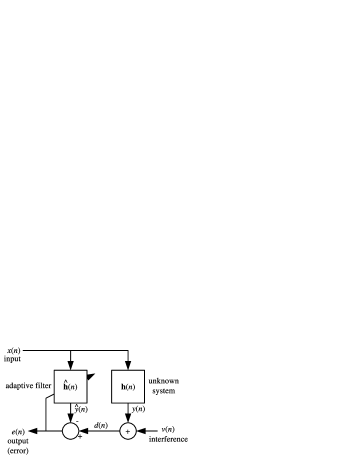
Figure 1: Block diagram of echo cancellation system.

Section II introduces existing gradient-adaptive learning rate algorithms and their limitations. Section III describes our proposed INLMS algorithm, followed by the results and discussion in Section IV. Section V concludes this paper.

II Gradient-Adaptive Learning Rate

Gradient-adaptive learning rate algorithms are based on the fact that when the adaptation rate is too small, the gradient tends to keep pointing in the same direction, while if it is too large, the gradient oscillates. Based on the behaviour of the stochastic gradient, it is thus possible to infer whether the learning rate must be increased or decreased, and several methods have been proposed in the past to adjust the learning based on the gradient.

These methods each have a control parameter that is used to determine the learning rate. In the case of [1, 2, 3], the control parameter is the learning rate itself. In the generalized normalized gradient descent (GNGD) algorithm [4] the (normalised) learning rate is:

$$\mu\left(n\right)=\frac{\mu_{0}\left\|\mathbf{x}\left(n\right)\right\|^{2}}{\left\|\mathbf{x}\left(n\right)\right\|^{2}+\epsilon\left(n\right)}$$ (3)

where $\epsilon\left(n\right)$ is the control parameter. Because the control parameter is adapted based on the NLMS stochastic gradient behaviour, it can only vary relatively slowly (typically requiring tens or hundreds of samples). For that reason, it is important for the optimal learning rate not to depend on rapid changes of the control parameter. We will show in the next section that none of the methods cited above can fulfil this condition for non-stationary sources.

II-A Analysis For Non-Stationary Signals

Under the assumption that $x\left(n\right)$ and $v\left(n\right)$ are zero-mean and uncorrelated to each other and that $v\left(n\right)$ is i.i.d., the theoretical optimal learning rate is equal to the residual-to-error ratio [5]:

$$\mu_{opt}\left(n\right)=\frac{E\left\{r^{2}\left(n\right)\right\}}{E\left\{e^{2}\left(n\right)\right\}}$$ (4)

where $r\left(n\right)=y\left(n\right)-\hat{y}\left(n\right)$ is the (unknown) residual echo and $e\left(n\right)$ is the error signal. It turns out that although the assumption on $v\left(n\right)$ is not verified for speech, (4) nonetheless remains a good approximation. Earlier gradient-adaptive algorithms vary $\mu\left(n\right)$ directly as a response to the behaviour of the gradient ($\mu\left(n\right)$ is the control parameter). It is a sensible thing to do if one assumes that $v\left(n\right)$ and $x\left(n\right)$ are stationary signals, because it means that both $E\left\{r^{2}\left(n\right)\right\}$ and $E\left\{e^{2}\left(n\right)\right\}$ vary slowly and, as a consequence, so does $\mu_{opt}\left(n\right)$. On the other hand, if the statistics of either $v\left(n\right)$ or $x\left(n\right)$ changes abruptly, then the algorithm is not capable of changing $\mu\left(n\right)$ fast enough to prevent the adaptive filter from diverging.

The GNGD algorithm provides more robustness to non-stationarity. If we examine $\epsilon\left(n\right)$ more closely, it is reasonable to surmise that (3) eventually converges to the optimal learning rate defined by (4). Assuming steady state behaviour ($\epsilon\left(n\right)$ is stable) and $\mu_{0}=1$, we find (by multiplying the left hand side numerator and denominator by $\gamma\left(n\right)$) that:

$$\frac{E\left\{r^{2}\left(n\right)\right\}}{E\left\{r^{2}\left(n\right)\right\}+\gamma\left(n\right)\epsilon\left(n\right)}=\frac{E\left\{r^{2}\left(n\right)\right\}}{E\left\{e^{2}\left(n\right)\right\}}$$ (5)

where $\gamma\left(n\right)=E\left\{r^{2}\left(n\right)\right\}/\left\|\mathbf{x}\left(n\right)\right\|^{2}$ is analogous to the filter misalignment. Assuming that $r\left(n\right)$ and $v\left(n\right)$ are zero-mean and uncorrelated to each other, we have $E\left\{e^{2}\left(n\right)\right\}=E\left\{r^{2}\left(n\right)\right\}+E\left\{v^{2}\left(n\right)\right\}$, which results in the relation $\epsilon\left(n\right)=E\left\{v^{2}\left(n\right)\right\}/\gamma\left(n\right)$. In other words, the optimal value for the gradient-adaptive parameter $\epsilon\left(n\right)$ depends on the filter misalignment and on the variance of the interference signal, but is independent of the variance of the input signal. Because $\epsilon\left(n\right)$ can only be adapted slowly over time, there is an implicit assumption in (3) that $E\left\{v^{2}\left(n\right)\right\}$ also varies slowly. While this is a reasonable assumption in some applications, it does not hold for scenarios like echo cancellation, where the interference is speech (double-talk) that can start or stop at any time.

III Proposed Algorithm For Non-Stationary Signals

In previous work [5], we proposed to use (4) directly to adapt the learning rate. While $E\left\{e^{2}\left(n\right)\right\}$ can easily be estimated, the estimation of the residual echo $E\left\{r^{2}\left(n\right)\right\}$ is difficult because one does not have access to the real filter coefficients. One reasonable assumption we can make is that:

$$E\left\{r^{2}\left(n\right)\right\} =\eta\left(n\right)E\left\{y^{2}\left(n\right)\right\}$$

$$\approx\eta\left(n{-}1\right)E\left\{\hat{y}^{2}\left(n\right)\right\}$$ (6)

where $\eta\left(n\right)$ is a form of normalised filter misalignment, and is easier to estimate than $E\left\{r^{2}\left(n\right)\right\}$ directly, because it is assumed to vary slowly as a function of time. Although it is possible to estimate $\eta\left(n\right)$ directly through linear regression, the estimation remains a difficult problem.

In this paper we propose to apply a gradient adaptive approach using $\eta\left(n\right)$ as the control parameter. By substituting (6) into (4), we obtain the learning rate:

$$\mu\left(n\right)=\min\left(\eta\left(n{-}1\right)\frac{\widehat{\sigma_{\hat{y}}^{2}}\left(n\right)}{\widehat{\sigma_{e}^{2}}\left(n\right)},1\right)$$ (7)

where $\widehat{\sigma_{\hat{y}}^{2}}\left(n\right)$ and $\widehat{\sigma_{e}^{2}}\left(n\right)$ are respectively the estimates for $E\left\{\hat{y}^{2}\left(n\right)\right\}$ and $E\left\{e^{2}\left(n\right)\right\}$ and the upper bound imposed by the $\min\left(\cdot\right)$ reflects the fact that the optimal learning rate can never exceed unity.

III-A Adaptation

In this paper we bypass the difficulty of estimating $\eta(n)$ directly and instead propose a closed-loop gradient adaptive estimation of $\eta(n)$. The parameter $\eta(n)$ is no longer an estimate of the normalised misalignment, but is instead adapted in closed-loop in such a way as to achieve a fast convergence of the adaptive filter.

As with other gradient-adaptive methods we update the control parameter $\eta(n)$ by computing the derivative of the squared error $\mathcal{E}\left(n\right)=\frac{1}{2}e^{*}\left(n\right)e\left(n\right)$, this time with respect to $\eta\left(n-1\right)$, using the chain derivation rule without the independence assumption [1, 6]:

$$\frac{\partial\mathcal{E}\left(n\right)}{\partial\eta\left(n{-}1\right)} =\frac{1}{2}\left(\frac{\partial e^{*}\left(n\right)}{\partial\eta\left(n{-}1\right)}e\left(n\right)+e^{*}\left(n\right)\frac{\partial e\left(n\right)}{\partial\eta\left(n{-}1\right)}\right)$$

$$=-\Re\left\{\frac{e\left(n\right)\mathbf{x}^{H}\left(n\right)\boldsymbol{\psi}\left(n-1\right)}{\left\|\mathbf{x}\left(n\right)\right\|^{2}}\right\}\frac{\widehat{\sigma_{\hat{y}}^{2}}\left(n\right)}{\widehat{\sigma_{e}^{2}}\left(n\right)}$$ (8)

where

$$\boldsymbol{\psi}\left(n\right)=\left[\mathbf{I}-\frac{\mu\left(n\right)\mathbf{x}\left(n\right)\mathbf{x}^{H}\left(n\right)}{\left\|\mathbf{x}\left(n\right)\right\|^{2}}\right]\boldsymbol{\psi}\left(n{-}1\right)+\mathbf{x}\left(n\right)e^{*}\left(n\right)$$ (9)

is a smoothed version of the gradient. We further rewrite the update of $\boldsymbol{\psi}\left(n\right)$ in (9) as

$$\boldsymbol{\psi}\left(n\right)= \boldsymbol{\psi}\left(n{-}1\right)-\frac{\mu\left(n\right)}{\left\|\mathbf{x}\left(n\right)\right\|^{2}}\mathbf{x}\left(n\right)\left[\mathbf{x}^{H}\left(n\right)\boldsymbol{\psi}\left(n{-}1\right)\right]$$

$$+\mathbf{x}\left(n\right)e^{*}\left(n\right)$$ (10)

so that it does not require a matrix-by-vector multiplication.

Based on this derivative, we propose the following exponential update of $\eta\left(n\right)$. We propose to use an exponential update in place of a more standard additive update since the misalignment has a large dynamic range; and we want the step size to scale with the value of $\eta\left(n\right)$. The exponential update is given as follows:

$$\eta\left(n\right)=\eta\left(n-1\right)\exp\left(\frac{\rho}{\widehat{\sigma_{e}^{2}}\left(n\right)}\frac{\partial\mathcal{E}\left(n\right)}{\partial\eta\left(n{-}1\right)}\right)$$ (11)

where $\rho$ is a step size and we have normalised the gradient $\frac{\partial\mathcal{E}\left(n\right)}{\partial\eta\left(n{-}1\right)}$ by $\widehat{\sigma_{e}^{2}}\left(n\right)$ to obtain a non-dimensional value.

It remains to estimate $\widehat{\sigma_{\hat{y}}^{2}}\left(n\right)$ and $\widehat{\sigma_{e}^{2}}\left(n\right)$. For $\widehat{\sigma_{e}^{2}}\left(n\right)$ we have the following recursive estimator with time constant $N$ ($\widehat{\sigma_{\hat{y}}^{2}}\left(n\right)$ is estimated similarly):

$$\hat{E}_{N}\left\{\left|e\left(n\right)\right|^{2}\right\}=\left(1{-}\frac{1}{N}\right)\hat{E}_{N}\left\{\left|e\left(n-1\right)\right|^{2}\right\}+\frac{1}{N}\left|e\left(n\right)\right|^{2}$$ (12)

The question then becomes what value of $N$ to use. To maximise stability, a conservative approach is to err on the side of picking the smallest $\widehat{\sigma_{\hat{y}}^{2}}\left(n\right)$ and the biggest $\widehat{\sigma_{e}^{2}}\left(n\right)$ out of the set of estimated obtained by varying $N$. For efficiency, we have chosen a subset of all possible $N$ values. The values $N=3$ and $N=10$ provide good short- to medium-term term estimation, though the algorithm is not very sensitive to the exact choice of $N$. For the estimation of $\widehat{\sigma_{e}^{2}}\left(n\right)$, we also include $N=1$ to make sure that even an instantaneous onset of interference cannot cause the filter to diverge. The complete algorithm is summarised in Fig. 2.

The last aspect that needs to be addressed is the initial condition. When the filter is initialised, all the weights are set to zero ($\hat{\mathbf{h}}\left(0\right)=\mathbf{0}$), which means that $\hat{y}\left(n\right)=0$ and no adaptation can take place in (7) and (8). In order to bootstrap the adaptation process, the learning rate $\mu\left(n\right)$ is set to a fixed constant (we use $\mu=0.25$) for a short time (until (7) gives $\mu\left(n\right)>0.1$). This ad hoc procedure is only necessary when the filter is initialised and is not required in case of echo path change. In practice, any method that provides a small initial convergence can be used.

$\begin{array}[]{rl}\hat{y}\left(n\right)=&\!\!\!\!=\hat{\mathbf{h}}\left(n{-}1\right)\mathbf{x}\left(n\right)\\ e\left(n\right)=&\!\!\!\!d\left(n\right)-\hat{y}\left(n\right)\\ \widehat{\sigma_{\hat{y}}^{2}}\left(n\right)=&\!\!\!\!\min\left(\hat{E}_{3}\left\{\left|\hat{y}\left(n\right)\right|^{2}\right\},\hat{E}_{10}\left\{\left|\hat{y}\left(n\right)\right|^{2}\right\}\right)\\ \widehat{\sigma_{e}^{2}}\left(n\right)=&\!\!\!\!\max\!\left(\!\hat{E}_{1}\!\left\{\!\left|e\left(n\right)\right|^{2}\!\right\}\!,\hat{E}_{3}\!\left\{\!\left|e\left(n\right)\right|^{2}\!\right\}\!,\hat{E}_{10}\!\left\{\!\left|e\left(n\right)\right|^{2}\!\right\}\!\right)\!\!\\ \mu\left(n\right)=&\!\!\!\!\min\left(\nu\left(n{-}1\right)\frac{\widehat{\sigma_{\hat{y}}^{2}}\left(n\right)}{\widehat{\sigma_{e}^{2}}\left(n\right)},1\right)\\ \hat{\mathbf{h}}\left(n\right)=&\!\!\!\!\hat{\mathbf{h}}\left(n{-}1\right)+\frac{\mu\left(n\right)}{\left\|\mathbf{x}\left(n\right)\right\|^{2}}e^{*}\left(n\right)\mathbf{x}\left(n\right)\\ \eta\left(n\right)=&\!\!\!\!\eta\left(n{-}1\right)\exp\!\left[\frac{\rho\widehat{\sigma_{\hat{y}}^{2}}\left(n\right)\Re\left\{e\left(n\right)\mathbf{x}^{H}\left(n\right)\boldsymbol{\psi}\left(n-1\right)\right\}}{\widehat{\sigma_{e}^{2}}\left(n\right)\left\|\mathbf{x}\left(n\right)\right\|^{2}\widehat{\sigma_{e}^{2}}\left(n\right)}\right]\\ \boldsymbol{\psi}\left(n\right)=&\!\!\!\!\boldsymbol{\psi}\left(n{-}1\right)-\frac{\mu\left(n\right)}{\left\|\mathbf{x}\left(n\right)\right\|^{2}}\mathbf{x}\left(n\right)\left[\mathbf{x}^{H}\left(n\right)\boldsymbol{\psi}\left(n{-}1\right)\right]\\ &\!\!\!\!+e^{*}\left(n\right)\mathbf{x}\left(n\right)\end{array}$

Figure 2: Summary of the INLMS algorithm

III-B Analysis

The adaptive learning rate described above is able to deal with both double-talk and echo path change without explicit modelling. From (7), we can see that when the interference changes abruptly, the denominator $\widehat{\sigma_{e}^{2}}\left(n\right)$ rapidly increases, causing an instantaneous decrease in the learning rate. In the case of a stationary interference, the learning rate depends on both the presence of an input signal and on the misalignment estimate. As the filter misalignment becomes smaller, the learning rate also becomes smaller. When the echo path changes, the gradient starts pointing steadily in the same direction, thus significantly increasing $\eta(n)$, which is a clear sign that the filter is no longer properly adapted.

In gradient adaptive methods [1, 2, 3], the implicit assumption is that both the near-end and the far-end signals are nearly stationary. We have shown that the GNGD algorithm [4] only requires the near-end signal to be nearly stationary. In the proposed INLMS method, both signals can be non-stationary, which is a requirement for double-talk robustness.

It should be noted that the per-sample complexity of the proposed algorithm only differs from the complexity of the “classic” algorithm in [1] by a constant ($O(1)$). For example, the total increase in complexity for the real-valued case is due to the increased cost of computing $\eta\left(n\right)$ and amounts to only 23 multiplications, 5 additions, 2 divisions and 1 exponential. Considering that the algorithms have an $O(L)$ complexity ($L$ is the filter length), the difference is negligible for any reasonable filter length.

IV Results And Discussion

We compare three algorithms:

• Direct learning rate adaptation [1]

• Generalized normalized gradient descent (GNGD) [4]

• INLMS algorithm (proposed)

In each case, we use a 32-second test sequence sampled at 8 kHz with an abrupt change in the unknown system $\mathbf{h}\left(n\right)$ at 16 seconds. The impulse responses are taken from ITU-T recommendation G.168 (impulse responses D.7 and D.9) and the filter length is 128 samples (16 ms). We choose $\rho=0.005$ since it gave good results over a wide range of operating conditions ($\rho$ should be inversely proportional to the filter length). To make the comparison fair, we also used the exponential update for the Direct method ($\rho=0.0005$ gave the best results) and the GNGD method ($\rho=0.005$ gave the best results).

We test the algorithms for three scenarios:

1. Both the input $x\left(n\right)$ and the interference $v\left(n\right)$ are white Gaussian noise (Fig. 3)

2. The input $x\left(n\right)$ is speech and the interference $v\left(n\right)$ is white Gaussian noise (Fig. 4)

3. Both the input $x\left(n\right)$ and interference $v\left(n\right)$ are speech (Fig. 5) with frequent overlap (double-talk)

The normalised misalignment is defined as:

$$\Lambda\left(n\right)=\left\|\hat{\mathbf{h}}\left(n\right)-\mathbf{h}\left(n\right)\right\|^{2}/\left\|\mathbf{h}\left(n\right)\right\|^{2}$$ (13)

In Fig. 3 we can see that all three algorithms successfully converge, albeit with differing convergence rates. In Fig. 4 it can be observed that the direct algorithm fails to converge for scenario 2 where the input is non-stationary, but GNGD and INLMS perform well. Finally in Fig. 5 we see that when the interference is non-stationary, only the proposed INLMS algorithm performs well.

Figure 3: Normalised misalignment for white Gaussian input and interference (scenario 1) with an abrupt change in the unknown system $\mathbf{h}\left(n\right)$ at 16 seconds. All algorithms converge.

Figure 4: Normalised misalignment for typical speech input and white Gaussian interference (scenario 2) with an abrupt change in the unknown system $\mathbf{h}\left(n\right)$ at 16 seconds. The direct algorithm diverges.

Figure 5: Normalised misalignment for typical speech input and interference (scenario 3) with an abrupt change in the unknown system $\mathbf{h}\left(n\right)$ at 16 seconds. Note that the direct method frequently diverges, and the GNGD method diverges less often, but still significantly between 3-4 seconds, at 6 seconds, 14 seconds and 31 seconds. All the divergence events are due to double-talk, except at 3-4 seconds, where only interference is present.

V Conclusion

We have proposed a new interference-normalised least mean square (INLMS) algorithm, based on the gradient-adaptive learning rate class of algorithms. We have demonstrated that unlike other gradient-adaptive methods, it is robust to non-stationarity of both the input and interference signals. This robustness is achieved by using a control parameter whose optimal value is independent of the power of the input and interference signals and instead depends only on the filter misalignment. This allows the instantaneous learning rate to react very quickly even though the control parameter cannot.

References

- [1] Benveniste, Adaptive algorithms and stochastic approximation, 1990.
- [2] V. Mathews and Z. Xie, “A stochastic gradient adaptive filter with gradient adaptive step size,” IEEE Trans. on Signal Processing, vol. 41, pp. 2075–2087, 1993.
- [3] W.-P. Ang and B. Farhang-Boroujeny, “A new class of gradient adaptive step-size LMS algorithms,” IEEE Trans. on Signal Processing, vol. 49, no. 4, pp. 805–810, 2001.
- [4] D. Mandic, “A generalized normalized gradient descent algorithm,” IEEE Signal Processing Letters, vol. 11, no. 2, pp. 115–118, 2004.
- [5] J.-M. Valin, “On adjusting the learning rate in frequency domain echo cancellation with double-talk,” IEEE Trans. on Audio, Speech and Language Processing, vol. 15, no. 3, pp. 1030–1034, 2007.
- [6] S. Goh and D. Mandic, “A class of gradient-adaptive step size algorithms for complex-valued nonlinear neural adaptive filters,” in Proceedings IEEE International Conference on Acoustics, Speech, and Signal Processing, vol. V, 2005, pp. 253–256.