Theoretical uncertainty of the supersymmetric dark matter relic density
from scheme and scale variations

Abstract

For particle physics observables at colliders such as the LHC at CERN, it has been common practice for many decades to estimate the theoretical uncertainty by studying the variations of the predicted cross sections with a priori unpredictable scales. In astroparticle physics, this has so far not been possible, since most of the observables were calculated at Born level only, so that the renormalization scheme and scale dependence could not be studied in a meaningful way. In this paper, we present the first quantitative study of the theoretical uncertainty of the neutralino dark matter relic density from scheme and scale variations. We first explain in detail how the renormalization scale enters the tree-level calculations through coupling constants, masses and mixing angles. We then demonstrate a reduction of the renormalization scale dependence through one-loop SUSY-QCD corrections in many different dark matter annihilation channels and enhanced perturbative stability of a mixed on-shell/$\overline{\rm DR}$ renormalization scheme over a pure $\overline{\rm DR}$ scheme in the top-quark sector. In the stop-stop annihilation channel, the Sommerfeld enhancement and its scale dependence are shown to be of particular importance. Finally, the impact of our higher-order SUSY-QCD corrections and their scale uncertainties are studied in three typical scenarios of the phenomenological Minimal Supersymmetric Standard Model with eleven parameters (pMSSM-11). We find that the theoretical uncertainty is reduced in many cases and can become comparable to the size of the experimental one in some scenarios.

I Introduction

Eighty years after Zwicky’s discovery of dark matter in the Coma galaxy cluster Zwicky:1933gu , its existence in the Universe is now well established from astronomical observations on many different length scales, but its nature is still unknown Klasen:2015uma . Nevertheless, precision measurements of the temperature fluctuations of the cosmic microwave background with the Planck satellite Ade:2015xua , supplemented by WMAP polarization data Bennett:2012zja , allow to deduce the global cold dark matter relic density in the Universe with previously unparalleled precision to

$$\Omega_{\mathrm{CDM}}h^{2}=0.1199\pm 0.0022.$$ (1)

Here, $h$ denotes the present Hubble expansion rate in units of 100 km s^-1 Mpc^-1.

An intriguing possibility for the nature of dark matter is a weakly interacting massive particle (WIMP), as it automatically leads to the correct relic abundance. In the absence of a suitable WIMP candidate within the Standard Model (SM), the arguably most popular candidate is a light supersymmetric (SUSY) particle, since SUSY has many other theoretical motivations ranging from a symmetry between fermions and bosons over a maximal extension of spacetime symmetry to a stabilization of the Higgs boson mass. In the case of the Minimal Supersymmetric SM (MSSM), the lightest SUSY particle (LSP) is typically the lightest neutralino, $\tilde{\chi}_{1}^{0}$, a mixture of the fermionic partners of the neutral electroweak gauge and CP-even Higgs bosons.

For a given set of parameters, the current neutralino relic density can be predicted by solving the Boltzmann equation describing the time evolution of its number density $n_{\chi}$,

$$\frac{\mathrm{d}n_{\chi}}{\mathrm{d}t}=-3Hn_{\chi}-\left\langle\sigma_{\mathrm{ann}}v\right\rangle\Big{[}n_{\chi}^{2}-\left(n_{\chi}^{\mathrm{eq}}\right)^{2}\Big{]}.$$ (2)

This nonlinear differential equation contains a term proportional to the Hubble expansion parameter $H$, which is responsible for the expansion of the Universe and thus for the dilution of matter. Particle physics enters through the second term on the right hand side, which is proportional to the thermally averaged annihilation cross section $\left\langle\sigma_{\mathrm{ann}}v\right\rangle$ and describes the annihilation and creation of neutralinos. This thermally averaged annihilation cross section includes all possible annihilation and coannihilation channels of neutralinos and other SUSY particles into SM particles.

After solving the Boltzmann equation numerically, the neutralino relic density is obtained via

$$\Omega_{\chi}h^{2}~{}=~{}\frac{m_{\chi}n_{\chi}}{\rho_{\mathrm{crit}}},$$ (3)

where $\rho_{\mathrm{crit}}$ is the critical density of the Universe. This value may then be compared to the very precise measurement given in Eq. (1) and allows the restriction of the MSSM parameter space. More details on the Boltzmann equation and its numerical treatment can be found in Refs. Gondolo:1990dk ; Griest:1990kh ; Edsjo:1997bg ; Harz:2012fz ; Harz:2014gaa .

During the last years, considerable progress has been made in the calculation of the neutralino relic density and other dark matter observables with respect to radiative corrections Baro:2007em ; Bringmann:2013oja ; Beneke:2012tg ; Hisano:2015rsa ; Drees:2009gt . More precisely, in recent publications we have calculated the full $\mathcal{O}(\alpha_{s})$ corrections to general gaugino (co)annihilations into quarks Herrmann:2007ku ; Herrmann:2009wk ; Herrmann:2009mp ; Herrmann:2014kma , to neutralino-stop coannihilation Harz:2012fz ; Harz:2014tma , and to stop-antistop annihilation into electroweak final states Harz:2014gaa . It is well known that such fixed-order calculations introduce an artificial (i.e. non-physical) dependence on the renormalization scheme and scale. For good reasons (preservation of gauge and Lorentz invariance), most perturbative calculations, including ours, employ dimensional regularization or (for the preservervation of SUSY invariance) dimensional reduction to regularize ultraviolet (and infrared) divergences. A variation of the renormalization scale leads then to a variation of the (co)annihilation cross sections and thus the predicted value for the relic density. For a calculation at $\mathcal{O}(\alpha_{s})$, the dependence on the scale is of $\mathcal{O}(\alpha_{s}^{2})$ and thus allows an estimate of the higher-order theoretical uncertainty.

In the present paper we analyze the renormalization scheme and scale dependence of the supersymmetric dark matter relic density in detail. With the help of three typical scenarios, covering all three classes of (co)annihilation channels mentioned above, we explain where and how the renormalization scale enters the calculations already at tree level and how its influence is reduced by higher-order SUSY-QCD corrections. This allows us to estimate for the first time the theoretical error on the calculation of the (co)annihilation cross sections and the neutralino relic density.

This paper is organized as follows: Sec. II is devoted to the discussion of technical aspects. We define a phenomenological MSSM with eleven free parameters (pMSSM-11), a mixed on-shell and $\overline{\rm DR}$ renormalization scheme, and analyze the origin and influence of the renormalization scale $\mu_{R}$ on our calculations at leading order (LO) and next-to-leading order (NLO). Furthermore, we discuss our treatment of Coulomb corrections and how we define and vary the associated Coulomb scale $\mu_{C}$ in our numerical analysis. In Sec. III, we then present numerical results for the various (co)annihilation cross sections and the predicted neutralino relic density for different choices of the renormalization scheme and scale in three pMSSM-11 benchmark scenarios. Finally, we conclude in Sec. IV.

II Setup and treatment of scales

We first discuss the setup of our numerical calculations, starting from the input parameters in the phenomenological MSSM (pMSSM), up to the calculation of the annihilation cross section $\sigma_{\rm ann}$ and the prediction of the relic density $\Omega_{\tilde{\chi}}h^{2}$.

As in our previous publications, we work in a pMSSM with eleven parameters, denoted as pMSSM-11 in the following and defined in the $\overline{\rm DR}$ scheme at the scale $\tilde{M}=1$ TeV according to the SPA convention AguilarSaavedra:2005pw . We identify this scale with our central renormalization scale $\mu_{R}^{\rm central}$. In particular, we parametrize the Higgs sector by the higgsino mass parameter $\mu$, the ratio of the vacuum expectation values of the two Higgs doublets $\tan\beta$, and the pole mass of the pseudoscalar Higgs boson $m_{A}$. The gaugino sector is fixed by the bino ($M_{1}$), wino ($M_{2}$) and gluino ($M_{3}$) mass parameters, which in our set-up are not related through any assumptions stemming from Grand Unified Theories. We define a common soft SUSY-breaking mass parameter $M_{\tilde{q}_{1,2}}$ for the first- and second-generation squarks. The third-generation squark masses are controlled by the parameter $M_{\tilde{q}_{3}}$ associated with sbottoms and left-handed stops and by the parameter $M_{\tilde{u}_{3}}$ for right-handed stops. The trilinear coupling in the stop sector is given by $A_{t}$, while the trilinear couplings of the other sectors, including $A_{b}$, are set to zero. Since the slepton sector is not at the center of our attention, it is parametrized by a single soft parameter $M_{\tilde{\ell}}$.

With this set of free parameters, we use the numerical program SPheno 3.3.3 Porod:2003um to obtain the associated physical mass spectrum at the scale $\tilde{M}$. In addition, SPheno is used to evolve all running parameters via the implemented renormalization group equations (RGEs) from the input scale $\tilde{M}\equiv\mu_{R}^{\rm central}$ to the renormalization scale $\mu_{R}$, where we want to evaluate the (co)annihilation cross sections. The results from other SUSY spectrum generators can differ, in particular in regions with important stop coannihilation, but these differences have been reduced by consistent implementations of two-loop RGEs Belanger:2005jk . Apart from the implicit dependence in some of the physical parameters to be discussed next, the renormalization scale also appears explicitly in our higher-order QCD calculations in the form of loop logarithms.

Our QCD calculations at next-to-leading order (NLO) and beyond are performed within a hybrid on-shell/$\overline{\rm DR}$ renormalization scheme, described in detail in Refs. Herrmann:2014kma ; Harz:2012fz ; Harz:2014tma . In the quark sector, the top- and bottom-quark masses are defined on-shell and in the $\overline{\rm DR}$ scheme, respectively, while all other quarks are taken as massless. Note that through the Yukawa coupling to (in particular the neutral pseudoscalar) Higgs-boson resonances, the bottom-quark mass can have a sizeable influence on the dark matter annihilation cross section and must therefore be treated with particular care. We obtain it from the SM $\overline{\rm MS}$ mass $m_{b}(m_{b})$, determined in an analysis of $\Upsilon$ sum rules, through evolution to the scale $\mu_{R}$, transformation to the SM $\overline{\rm DR}$ and then MSSM $\overline{\rm DR}$ scheme Herrmann:2014kma ; Harz:2012fz . In the squark sector, we have five independent parameters

$$m_{\tilde{t}_{1}},\quad m_{\tilde{b}_{1}},\quad m_{\tilde{b}_{2}},\quad A_{t}\quad\mathrm{and}\quad A_{b}=0.$$ (4)

This choice makes our renormalization scheme applicable to all annihilation and coannihilation processes, where squarks play an important role. The lighter stop mass and the two sbottom masses are taken to be on-shell, while the stop and sbottom trilinear coupling parameters are taken in the $\overline{\rm DR}$ scheme. From these parameters, we compute as dependent quantities the stop and sbottom mixing angles $\theta_{\tilde{t}}$ and $\theta_{\tilde{b}}$ in the $\overline{\rm DR}$ scheme at the scale $\mu_{R}$ as well as the on-shell masses of the first- and second generation squarks and $m_{\tilde{t}_{2}}$ for the heavier stop Harz:2012fz . The strong coupling constant $\alpha_{s}(\mu_{R})$ is renormalized in the MSSM $\overline{\rm DR}$ scheme with six active flavors and obtained after evolution of the world-average, five-flavor SM $\overline{\rm MS}$ value at the $Z^{0}$-boson mass to the renormalization scale $\mu_{R}$ and an intermediate transformation to the SM $\overline{\rm DR}$ scheme Harz:2014tma . In our calculaton, all running parameters are thus evaluated at the scale $\mu_{R}$, which we can then vary in order to study the scale dependence of the (co)annihilation cross sections and consequently the neutralino relic density. In the following numerical analysis, we will vary the renormalization scale between $\mu_{R}=0.5$ TeV and $\mu_{R}=2$ TeV, corresponding to a factor $1/2$ or $2$, respectively, as compared to the central scale $\mu_{R}^{\rm central}$. Note that since we are studying QCD corrections, we are not interested in the effects from the running of electroweak parameters. We therefore read all SUSY parameters except $A_{t}$ and $A_{b}$ from the spectrum obtained at the central scale.

In our calculation of stop-antistop annihilation into electroweak (EW) final states, we also include the Coulomb corrections connected to the exchange of potential gluons in the initial state. As outlined in Ref. Harz:2014gaa , the exchange of $n$ potential gluons comes with a factor $(\alpha_{s}/v)^{n}$. In the region of low relative velocity $v\lesssim\alpha_{s}$ between the incoming stop-antistop pair, this factor can become large and spoil the convergence of the perturbative series in $\alpha_{s}$. Hence, these multiple gluon exchanges have to be resummed to all orders in perturbation theory in order to get a reliable result. Following Ref. Kiyo:2008bv , this can be done via

$$\sigma^{\mathrm{Coul}}\big{(}\tilde{t}_{1}\tilde{t}^{*}_{1}\rightarrow\mathrm{EW}\big{)}=\frac{4\pi}{vm_{\tilde{t}_{1}}^{2}}$$ (5)

$$\times\Im\Big{\{}G^{[1]}\big{(}\mathbf{r}=0;\sqrt{s}+i\Gamma_{\tilde{t}_{1}},\mu_{C}\big{)}\Big{\}}\sigma^{\mathrm{LO}}\big{(}\tilde{t}_{1}\tilde{t}^{*}_{1}\rightarrow\mathrm{EW}\big{)}.$$

As apparent from Eq. (5), we encounter a residual scale dependence of our final result $\sigma^{\mathrm{Coul}}$ on the Coulomb scale $\mu_{C}$ connected to the dimensional regularization of the associated color-singlet Greens function $G^{[1]}$, which is UV-divergent at the origin $\mathbf{r}=0$ Beneke:1999zr . The latter can be obtained as a solution to the would-be stoponium Schrödinger equation

$$\Big{[}H^{[1]}-\big{(}\sqrt{s}+i\Gamma_{\tilde{t}_{1}}\big{)}\Big{]}G^{[1]}\big{(}\mathbf{r};\sqrt{s}+i\Gamma_{\tilde{t}_{1}},\mu_{C}\big{)}=\delta^{(3)}(\mathbf{r})$$ (6)

with the Hamilton operator

$$H^{[1]}=-\frac{1}{m_{\tilde{t}_{1}}}\Delta+2m_{\tilde{t}_{1}}+V^{[1]}(\mathbf{r})$$ (7)

and the color-singlet Coulomb potential $V^{[1]}(\mathbf{r})$. At NLO, $V^{[1]}(\mathbf{r})$ includes corrections up to $\mathcal{O}(\alpha_{s}^{2})$. Following the results given in Ref. Harz:2014gaa , Eq. (5) adds up terms of the order $\mathcal{O}((\alpha_{s}/v)^{n})$ and $\mathcal{O}((\alpha_{s}^{2}/v))^{n})$ up to infinite order in $n$. At this precision $\mu_{C}$ can be treated independently from the renormalization scale $\mu_{R}$ connected to the hard part of the process Kiyo:2008bv . We choose

$$\mu_{C}^{\rm central}=\max\{\mu_{B},2m_{\tilde{t}_{1}}v\}$$ (8)

as our central Coulomb scale in order to minimize potentially large logarithms Beneke:2010da . Here, $\mu_{B}=C_{F}\alpha_{s}m_{\tilde{t}_{1}}$ corresponds to the inverse Bohr radius, the characteristic energy scale of the stop-antistop bound state. We describe in detail how we combine the uncertainties due to variations of $\mu_{R}$ and $\mu_{C}$ in Sec. III.2.

For values of $\mu_{C}$ below $\mu_{B}$, the authors of Ref. Beneke:2005hg encountered an instability of the convergence of the perturbative solution used here against an exact numerical solution of Eq. (6). This instability has been traced back to large higher-order logarithmic corrections which tend to blow up for $\mu_{C}\ll\mu_{B}$. For the scenarios presented here we have explictly checked that the variation does not become too large and, hence, does not yield an overestimation of the corresponding scale uncertainty. This should be kept in mind for the results shown further below. Finally note that the solution $G^{[1]}$ to Eq. (6) expanded up to $\mathcal{O}(\alpha_{s})$ takes the form

$$\Im\Big{\{}G^{[1]}\big{(}0;\sqrt{s}+i\Gamma_{\tilde{t}_{1}},\mu_{C}\big{)}\Big{\}}=$$ (9)

$$m_{\tilde{t}_{1}}^{2}\Im\Big{\{}\frac{v}{4\pi}\Big{[}i+\frac{\alpha_{s}(\mu_{C})C_{F}}{v}\Big{(}\frac{i\pi}{2}+\ln\frac{\mu_{C}}{2m_{\tilde{t}_{1}}v}\Big{)}+\mathcal{O}(\alpha_{\mathrm{s}}^{2})\Big{]}\Big{\}}.$$

Hence, the explicit scale dependence of the Greens function drops out of the Coulomb corrected cross section at $\mathcal{O}(\alpha_{s})$ and re-enters first at NNLO. However, whereas $m_{\tilde{t}_{1}}$, which we choose to renormalize in the on-shell scheme, remains scale independent, Eq. (9) still features an implicit dependence on $\mu_{C}$ due to the strong coupling $\alpha_{s}(\mu_{C})$.

As a final remark, let us stress again that, although the renormalization scale appears explicitly only at the one-loop level, also the tree-level result will vary with the scale $\mu_{R}$. First, this is due to taking the values of $A_{t}$ and $A_{b}$ at this scale and deriving from them, e.g., the squark mixing angles, which enter the calculation already at the tree level whenever top or bottom squarks are involved. As already mentioned, also the bottom-quark mass and the strong coupling constant are taken as MSSM $\overline{\mathrm{DR}}$ parameters and thus directly scale-dependent. The former appears at the tree level in Yukawa couplings, e.g., in the Higgs funnel of gaugino annihilation into bottom quark pairs, and the latter enters at tree level in stop coannihalation into top quarks and gluons, as we explain in more detail in the next Section.

III Numerical results

Table 1: pMSSM-11 input parameters for three selected reference scenarios. All parameters except $\tan\beta$ are given in GeV.

	$\quad\tan\beta\quad$	$\quad\mu\quad$	$\quad m_{A}\quad$	$\quad M_{1}\quad$	$\quad M_{2}\quad$	$\quad M_{3}\quad$	$\quad M_{\tilde{q}_{1,2}}\quad$	$\quad M_{\tilde{q}_{3}}\quad$	$\quad M_{\tilde{u}_{3}}\quad$	$\quad M_{\tilde{\ell}}\quad$	$\quad A_{t}\quad$
A	13.4	1286.3	1592.9	731.0	766.0	1906.3	3252.6	1634.3	1054.4	3589.6	-2792.3
B	27.0	2650.8	1441.5	1300.0	1798.4	1744.8	2189.7	2095.3	1388.0	1815.5	-4917.5
C	5.8	2925.8	948.8	335.0	1954.1	1945.6	3215.1	1578.0	609.2	3263.9	3033.7

Table 2: Gaugino and stop masses, the decomposition of the lightest neutralino, and selected observables corresponding to the reference scenarios of Tab. 1. All masses are given in GeV.

	$m_{\tilde{\chi}^{0}_{1}}$	$m_{\tilde{\chi}^{0}_{2}}$	$m_{\tilde{\chi}^{\pm}_{1}}$	$m_{\tilde{\chi}^{\pm}_{2}}$	$m_{\tilde{t}_{1}}$	$m_{\tilde{t}_{2}}$	$Z_{1\tilde{B}}$	$Z_{1\tilde{W}}$	$Z_{1\tilde{H}_{1}}$	$Z_{1\tilde{H}_{2}}$	$m_{h^{0}}$	$\Omega_{\tilde{\chi}^{0}_{1}}h^{2}$	$\mathrm{BR}(b\rightarrow s\gamma)$
A	738.1	802.5	802.4	1295.3	1032.1	1682.0	- 0.996	0.049	-0.059	0.037	126.5	0.1248	$3.0\cdot 10^{-4}$
B	1306.3	1827.0	1827.2	2640.0	1361.7	2157.3	-1.000	0.002	-0.024	0.013	123.7	0.1134	$3.1\cdot 10^{-4}$
C	338.3	1996.6	1996.7	2909.0	376.3	1554.0	1.000	0.000	0.016	-0.004	121.7	0.1193	$3.49\cdot 10^{-4}$

Table 3: Most relevant (co)annihilation channels in the reference scenarios of Tab. 1. Channels which contribute less than 1% to the thermally averaged cross section and/or are not implemented in our code are not shown.

		A	B	C
$\tilde{\chi}^{0}_{1}\tilde{\chi}^{0}_{1}\to$	$t\bar{t}$	2%		16%
	$b\bar{b}$	9%
$\tilde{\chi}^{0}_{1}\tilde{\chi}^{0}_{2}\to$	$t\bar{t}$	3%
	$b\bar{b}$	23%
$\tilde{\chi}^{0}_{1}\tilde{\chi}^{\pm}_{1}\to$	$t\bar{b},\bar{t}b$	43%
$\tilde{\chi}^{0}_{1}\tilde{t}_{1}\to$	$th^{0}$		1%	23%
	$tg$		6%	23%
	$tZ^{0}$			5%
	$bW^{+}$			11%
$\tilde{t}_{1}\tilde{t}^{*}_{1}\to$	$h^{0}h^{0}$		12%	5%
	$h^{0}H^{0}$		11%
	$Z^{0}A^{0}$		7%
	$W^{\pm}H^{\mp}$		13%
	$Z^{0}Z^{0}$		8%	2%
	$W^{+}W^{-}$		14%	3%
Total		80%	72%	88%

In this Section, we present numerical results for three reference scenarios within the pMSSM-11, which we introduce in Tab. 1. Table 2 shows the corresponding relevant gaugino and squark masses, the neutralino decomposition as well as the obtained mass of the lightest neutral (and thus SM-like) Higgs boson, the neutralino relic density computed at the tree level with micrOMEGAs 2.4.1 Belanger:2001fz , and the important branching ratio of the rare $B$-meson decay $b\to s\gamma$ computed with SPheno Porod:2003um . Remember that in particular $m_{\tilde{t}_{2}}$ is a dependent parameter in our setup and thus calculated by us (cf. Sec. II). To complete the information about the scenarios, we summarize in Tab. 3 the most relevant (co)annihilation channels. As the physics behind these three scenarios is quite different, we devote an individual subsection to each of them.

Our scenarios A, B, and C are taken from the earlier publications Ref. Herrmann:2014kma , Ref. Harz:2014gaa and Ref. Harz:2014tma , respectively, for easy comparability and to improve on these results by additional estimates of the theoretical uncertainties. In addition to the constraint Eq. (1) from the relic density, we have also verified those from the Higgs mass and the inclusive branching ratio of the decay $b\to s\gamma$. Let us note that, while in the previous papers the trilinear coupling was entered as $T_{t}$, we now use the value of $A_{t}=T_{t}/Y_{t}$ ($Y_{t}$ being the top Yukawa coupling) due to a change in the SPheno version. We have verified that this change together with the replacement $T_{t}\to A_{t}$ has neither a significant impact on the obtained mass spectrum nor on the prediction of the relic density.

III.1 Gaugino (co)annihilation

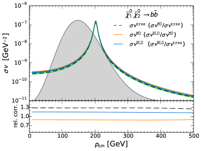
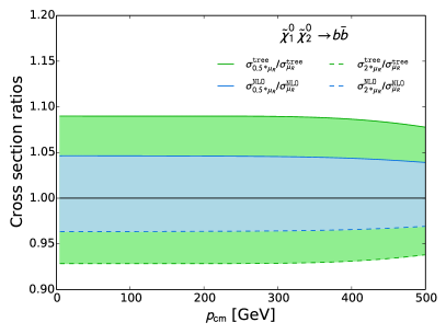
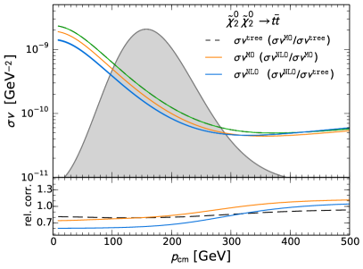
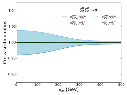
Figure 1: Cross sections of the neutralino annihilation processes $\tilde{\chi}^{0}_{1}\tilde{\chi}^{0}_{2}\to b\bar{b}$ (top) and $\tilde{\chi}^{0}_{2}\tilde{\chi}^{0}_{2}\to t\bar{t}$ (bottom) as a function of the center-of-mass momentum $p_{\rm cm}$ in scenario A. The left plots show the annihilation cross sections calculated at the tree level (black dashed lines) and at the one-loop level (blue solid lines) including the corresponding uncertainties from variations of the renormalization scale $\mu_{R}$ between $\mu_{R}^{\rm central}/2$ and $2\mu_{R}^{\rm central}$ (green and blue shaded bands). We also indicate the values obtained with micrOMEGAs (orange solid lines). The right plots show the cross sections normalized to their values obtained with the central renormalization scale $\mu_{R}^{\rm central}=1$ TeV.

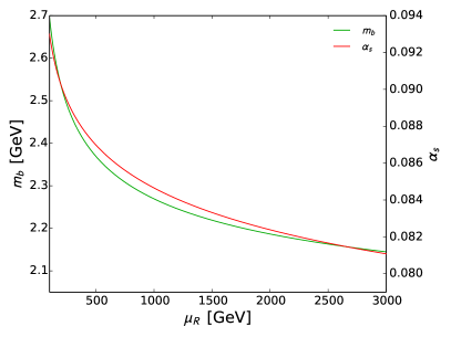
Figure 2: Dependence of the bottom-quark mass $m_{b}$ (green line, left ordinate) and of the strong coupling constant $\alpha_{s}$ (red line, right ordinate) on the renormalization scale $\mu_{R}$ in the MSSM $\overline{\rm DR}$ scheme in scenario A.

We begin our numerical investigation by studying the cross section of the process $\tilde{\chi}_{1}^{0}\tilde{\chi}_{2}^{0}\rightarrow b\bar{b}$ in scenario A. We do not reproduce here a detailed phenomenological discussion of this scenario, as it can be found in Ref. Herrmann:2014kma . The upper left graph of Fig. 1 presents the cross section times the relative neutralino velocity $v$ for the mentioned process calculated with CalcHEP-based Pukhov:2004ca micrOMEGAs Belanger:2001fz (orange solid line), DM@NLO at tree level (black dashed line), and NLO (blue solid line) at $\mu_{R}^{\rm central}=1$ TeV as a function of the center-of-mass momentum $p_{\mathrm{cm}}$. Note that in our code the widths of unstable particles are always active, whereas in micrOMEGAs they are switched on only in a rather narrow interval around the resonance. In order to compare our calculation with the one implemented in micrOMEGAs, we have modified the treatment of the width in CalcHEP such that it is taken into account over the full range of $p_{\mathrm{cm}}$. For the calculation of the relic density, however, we have not modified the treatment of the width in CalcHEP. The general shape of the curves is dominated by a large $A^{0}$ resonance at $p_{\mathrm{cm}}\approx 200$ GeV in the vicinity of the maximum of the thermal dark matter velocity distribution (gray shaded contour), which makes this process relevant for neutralino relic density calculations (see Tab. 3). The difference between the two tree-level calculations can be traced back to the fact that micrOMEGAs uses effective masses and couplings, while we do not. The lower subplot shows the ratios of the three cross sections (cf. the second items in the legend). The new features in this plot with respect to the analysis presented in Ref. Herrmann:2014kma are the green and blue shaded bands associated with the dashed black and blue solid lines. These bands are limited by calculations with renormalization scales of $\mu_{R}=0.5$ TeV and $\mu_{R}=2$ TeV, respectively, so that the area between them indicates the theoretical uncertainty due to renormalization scale variations. Remember that the input scale used for the pMSSM-11 parameters $\tilde{M}\equiv\mu_{R}^{\rm central}=1$ TeV remains unchanged, as we do not want to change the underlying scenario (see Sec. II). We observe a rather large scale dependence of our tree-level cross section (green shaded band) and a smaller dependence at NLO (blue shaded band). The bands overlap, as is visible at around $p_{\mathrm{cm}}=100$ GeV, but the central NLO result does not fall in the tree-level band. In other words, the impact of NLO radiative corrections on the final result is larger than the uncertainty estimated from the LO scale dependence. This is typical for a process that is of purely electroweak origin at LO. The orange micrOMEGAs results lies outside of both bands. This means that our full NLO cross section differs from the effective tree-level result obtained by micrOMEGAs even after including the scale uncertainty.

To enhance the visibility of the scale uncertainties, in particular near the resonance, we show in the upper right plot of Fig. 1 ratios of the tree-level and NLO cross sections at $\mu_{R}=(0.5;2)\times\mu_{R}^{\rm central}$ over the central results. We find an increase of $\sim 9\%$ of the tree-level cross section when changing from $\mu_{R}=1$ TeV to $\mu_{R}=0.5$ TeV and a decrease of $\sim 7\%$ when working with $\mu_{R}=2$ TeV (green shaded band). The shifts are almost constant and decrease only slightly at high $p_{\mathrm{cm}}$. The reason is that the dominant subprocess here is the $s$-channel process $\tilde{\chi}_{1}^{0}\tilde{\chi}_{2}^{0}\rightarrow A^{0}\rightarrow b\bar{b}$, as we now explain: The coupling $A^{0}b\bar{b}$ is of Yukawa type and proportional to $m_{b}$. Therefore, the total subprocess is proportional to $m_{b}^{2}$. As the bottom mass is handled as a $\overline{\mathrm{DR}}$ parameter in our code (cf. Sec. II), its scale dependence directly translates to the cross section in this case.

This scale dependence is illustrated in Fig. 2. More precisely, the ratios $(\frac{m_{b}(\mu_{R}=2\,\mathrm{TeV})}{m_{b}(\mu_{R}=1\,\mathrm{TeV})})^{2}\approx 0.93$ and $(\frac{m_{b}(\mu_{R}=0.5\,\mathrm{TeV})}{m_{b}(\mu_{R}=1\,\mathrm{TeV})})^{2}\approx 1.09$ reflect the observed shifts very well. The slight decrease of these shifts at high $p_{\mathrm{cm}}$ in the upper right plot of Fig. 1 has a related origin. Since the relative contributions of different subprocesses depend on $p_{\mathrm{cm}}$ (see Tab. IV in Ref. Herrmann:2014kma ), the subprocess $\tilde{\chi}_{1}^{0}\tilde{\chi}_{2}^{0}\rightarrow A^{0}\rightarrow b\bar{b}$ becomes less dominant at high $p_{\mathrm{cm}}$, and other subprocesses, which are not proportional to $m_{b}$, start to contribute as well. Hence the influence of $m_{b}$ and its scale dependence on the whole process decreases. The scale dependence is reduced at NLO, as shown by the blue shaded band in the upper right plot of Fig. 1. This is exactly as expected: Including virtual corrections, in particular vertex corrections to the $A^{0}b\bar{b}$ Yukawa coupling, reduces the scale depence of the resulting cross section. The remaining uncertainty amounts to less than five percent.

We continue with the lower part of Fig. 1. The lower left plot shows the cross section of the non-resonant process $\tilde{\chi}_{2}^{0}\tilde{\chi}_{2}^{0}\rightarrow t\bar{t}$. In this case, the Yukawa couplings contain the top-quark mass, which is defined as a pole mass in our code and therefore scale independent. Due to its rather small cross section, this process is irrelevant in terms of relic density calculations and hence not listed in Tab. 3. Nevertheless it proves useful for illustrating the scale dependence of our code.

As before, the black dashed and blue solid lines are associated with the green and blue shaded bands corresponding to the tree-level and NLO cross sections, respectively, at $\mu_{R}=0.5$ TeV and $\mu_{R}=2$ TeV. However, these bands are almost invisible in this case, as they overlap with the original lines. This fact indicates a much smaller scale dependence of the process than previously, which is confirmed in the lower right plot of Fig. 1. The (purely electroweak) tree-level cross section is basically scale independent, i.e. the green shaded band coincides with a nearly constant value of one. At NLO (blue shaded band), the scale dependence is now increased, to up to two percent at low $p_{\mathrm{cm}}$. This is due to the scale dependence of $\alpha_{s}$ introduced by our SUSY QCD corrections and depicted in Fig. 2. Although this seems to worsen the reliability of the calculation at first sight, the contrary is true: only at NLO it becomes possible to quantify the theoretical error for the first time. In this channel, the NLO corrections tend to decrease the cross section, i.e. the blue solid line lies below the black dashed line and the NLO/LO ratio below one. This effect is reduced at higher $p_{\mathrm{cm}}$, so that the NLO scale dependence decreases significantly. Note that an explicit dependence on $\alpha_{s}$ is also introduced in the process $\tilde{\chi}_{1}^{0}\tilde{\chi}_{2}^{0}\rightarrow b\bar{b}$ discussed at the beginning of this Section. There, however, it is completely overshadowed by the dominant scale dependence of $m_{b}$. We will encounter similar competing scale dependencies (e.g. on $\alpha_{s}$ and $A_{t}$) in other processes later.

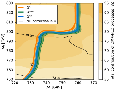
Figure 3: Cosmologically preferred regions with respect to Eq. (1) in the $M_{1}$-$M_{2}$-plane surrounding scenario A (white star). The solid bands correspond to the limits of Eq. (1), while the shaded bands include an additional variation of the renormalization scale $\mu_{R}$ between $\mu_{R}^{\rm central}/2$ and $2\mu_{R}^{\rm central}$. The shades of yellow indicate the percentages of the total annihilation cross section which have been corrected in our calculation, while the solid lines represent contours of the relative correction to the relic density in percent.

We close this subsection with a discussion of the scale dependence of the neutralino relic density. In Fig. 3 we show the relic density in the $M_{1}$–$M_{2}$-plane surrounding scenario A. The three colored, solid lines represent the part of the parameter space which leads to a neutralino relic density compatible with the Planck limits given in Eq. (1). These lines are rather thin, which reflects the high precision of the Planck measurement. For the orange line we used the standard micrOMEGAs routine, the green one corresponds to our tree-level calculation, and the blue one represents our full one-loop calculation. The last two lines are surrounded by green and blue shaded bands, which correspond to changing the renormalization scale to 0.5 or 2 TeV. The shades of yellow denote the relative fraction of processes we correct with DM@NLO and the black lines the relative correction to the relic density. We observe that the tree-level and NLO results clearly overlap within the scale uncertainty. This is not unexpected, as the relative shift from micrOMEGAs (and similarly LO) to NLO in this scenario happens to be rather small ($5-10$%). Furthermore note that the scale dependence of the relic density reduces at NLO, i.e. the blue shaded band surrounding the blue line is smaller than the green band surrounding the green line. This can be understood as follows: The processes we correct with DM@NLO account for 80% in this part of the parameter space. The most important ones are $\tilde{\chi}_{1}^{0}\tilde{\chi}_{2}^{0}\rightarrow b\bar{b}$, $\tilde{\chi}_{1}^{0}\tilde{\chi}_{1}^{0}\rightarrow b\bar{b}$ and $\tilde{\chi}_{1}^{+}\tilde{\chi}_{1}^{0}\rightarrow t\bar{b}$ (cf. Tab. 3 and Ref. Herrmann:2014kma ) and mainly take place via $s$-channel Higgs exchanges. The tree-level couplings entering these processes all contain Yukawa couplings proportional to the bottom quark $m_{b}$. Therefore, the discussion of the cross section of the process $\tilde{\chi}_{1}^{0}\tilde{\chi}_{2}^{0}\rightarrow b\bar{b}$ above translates to the relic density, and the dominant source of scale dependence is again the $\overline{\mathrm{DR}}$ bottom mass. This scale dependence is decreased at NLO, when vertex and other NLO corrections are included. Our NLO result (blue solid line) differs from the micrOMEGAs result (orange solid curve) even after including the scale uncertainty (blue shaded band), which we have already previously traced back to different treatments of the third-generation quark masses Herrmann:2014kma .

An extraction of the pMSSM-11 parameters from the Planck relic density with micrOMEGAs would lead to $M_{1}=731\pm 1$ GeV and $M_{2}=766\pm 1$ GeV and a precision of about 1 per mille, while our calculations would rather imply $M_{1}=731\pm 2$ GeV and $M_{2}=759\pm 2$ GeV, i.e. a shift in $M_{2}$ by 7 GeV or 1% with an uncertainty of two per mille, two times bigger than naively believed.

III.2 Stop-antistop annihilation

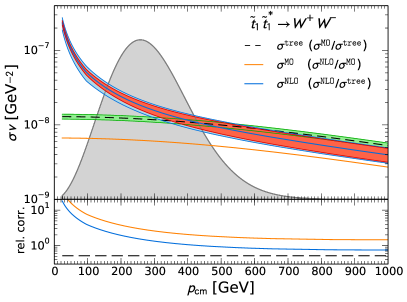
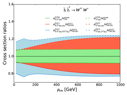
Figure 4: Cross sections of the stop-antistop annihilation process $\tilde{t}_{1}\tilde{t}_{1}^{*}\to W^{+}W^{-}$ as a function of the center-of-mass momentum $p_{\rm cm}$ in scenario B. The left plot shows the annihilation cross sections calculated at the tree level (black dashed line) and at the one-loop level with Coulomb resummation (blue solid line) including the corresponding uncertainties from simultaneous variations of the renormalization scale $\mu_{R}$ and the Coulomb scale $\mu_{C}$ by factors of two around the central scales (green and blue shaded bands). Also shown is the uncertainty from variations of $\mu_{R}$ alone (red shaded band). We also indicate the value obtained with micrOMEGAs (orange solid line). The right plot shows the cross sections normalized to their values obtained with central renormalization and Coulomb scales $\mu_{R}^{\rm central}$ and $\mu_{C}^{\rm central}$.

We continue our analysis with scenario B, where stop-antistop annihilation is dominant (see Tab. 3). This scenario has been introduced and studied as scenario II in Ref. Harz:2014gaa . As an example, we investigate in the left plot of Fig. 4 the cross section of the process $\tilde{t}\tilde{t}^{*}\rightarrow W^{+}W^{-}$. The color codes for the micrOMEGAs (orange solid lines) and our central tree-level cross sections (black dashed line) are as before. Our full result (blue solid line) includes now NLO and Coulomb corrections, calculated at a renormalization scale of $\mu_{R}^{\rm central}=1$ TeV and a Coulomb scale of $\mu_{C}^{\rm central}=\max\{\mu_{B},2m_{\tilde{t}_{1}}v\}$ (cf. Sec. II).

The Coulomb corrections lead to a strong enhancement of the cross section of up to a factor of ten in particular at small $p_{\mathrm{cm}}$, as observed also in Figs. 6 and 8 of Ref. Harz:2014gaa . The Coulomb enhancement region overlaps significantly with the Boltzmann velocity distribution and thus contributes in an important way to the dark matter relic density. At large $p_{\rm cm}$, our full cross section falls below the one at tree level, leading to a $K$-factor of about 0.75 (cf. the left lower subplot in Fig. 4), and approaches the one in micrOMEGAs, but still differs from it due to different definitions of the top-quark mass. Their effect is, however, reversed and reduced by the one-loop corrections included in our full calculation.

As before, the green shaded band indicates the theoretical uncertainty of the tree-level result induced by variations of $\mu_{R}$ by factors of two. Here, the renormalization scale influences the tree-level cross section through the trilinear coupling $A_{t}$, on which the squark mixing matrices and thus the squark-squark-vector couplings of the dominant $t$- and $u$-channel squark-exchange subprocesses depend (cf. table IV in Ref. Harz:2014gaa ). If we keep $A_{t}$ fixed, the tree-level result becomes scale independent. We show the scale dependence of $A_{t}$ explicitly in Fig. 5.

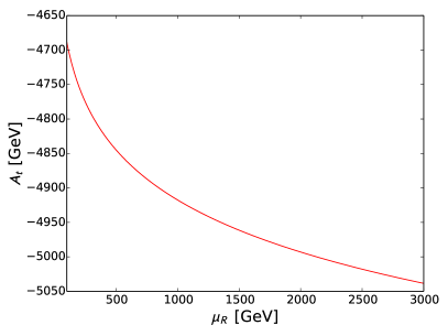
Figure 5: Dependence of the trilinear coupling $A_{t}$ (red line) on the renormalization scale $\mu_{R}$ in scenario B.

In contrast, the blue shaded band in Fig. 4 now indicates the simultaneous variations of $\mu_{R}$ and $\mu_{C}$ by factors of two, i.e. from $\mu_{R}=\mu_{C}=0.5$ TeV to 2 TeV. This is the most conservative procedure to combine the two uncertainties, as can be seen from the dependence of the relic density on the two scales in Fig. 6.

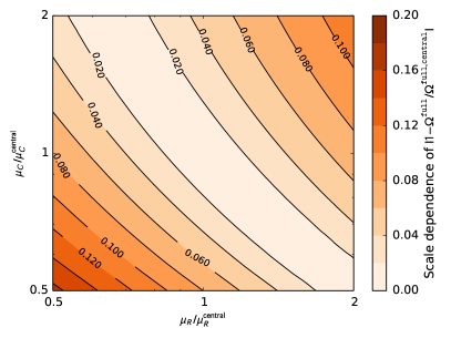
Figure 6: Dependence of the relic density on the scales $\mu_{R}$ and $\mu_{C}$ in scenario B.

The dependence of our full cross section on $\mu_{R}$ alone is shown in Fig. 4 as a red shaded band. As one observes from the right-hand plot, it dominates the full theoretical uncertainty with an error of about $\pm 20\%$ at large $p_{\rm cm}$. The one-loop corrections there depend implicitly on $\mu_{R}$ through the newly introduced strong coupling constant $\alpha_{s}$ and explicitly (logarithmically) through the NLO corrections. In contrast to scenario A, these dependencies are sizeable in scenario B and not completely overshadowed by the leading-order dependence on $m_{b}$ discussed there. The uncertainty induced by $\mu_{R}$ on the full cross section falls to the level of about $\pm 7\%$ at low $p_{\rm cm}$, where it becomes comparable to the constant tree-level uncertainty. However, there the Coulomb corrections and their theoretical uncertainty, induced by variations of $\mu_{C}$, become important as expected, and they increase the full higher-order theoretical uncertainty again to about $\pm 20\%$.

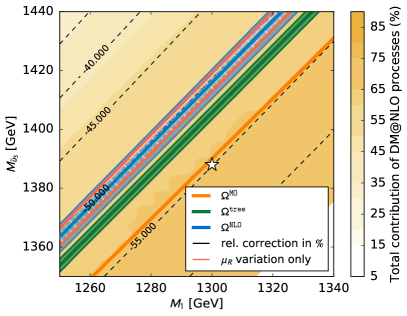
Figure 7: Cosmologically preferred regions with respect to Eq. (1) in the $M_{1}$-$M_{\tilde{u}_{3}}$-plane surrounding scenario B (white star). The solid bands correspond to the limits of Eq. (1), while the shaded bands include additional variations of the renormalization scale $\mu_{R}$ and the Coulomb scale $\mu_{C}$ by factors of two around the central scales. The shades of yellow indicate the percentages of the total annihilation cross section which have been corrected in our calculation, while the dashed lines represent contours of the relative correction to the relic density in percent.

To conclude this subsection, we show in Fig. 7 a relic-density scan in the $M_{1}-M_{\tilde{u}_{3}}$ plane around our representative scenario B (white star). In the whole region, our calculations correct more than 60% of the contributing subprocesses (shades of yellow). The tree-level result (green line) differs again visibly from the micrOMEGAs result (orange line) defined in a different way and exhibits only a small renormalization scale dependence (green shaded band) induced by the trilinear coupling $A_{t}$. The combined scale uncertainty from variations of $\mu_{R}$ and $\mu_{C}$ of the full result (blue shaded band) is larger and significantly broadens the 1$\sigma$-band representing the experimental error from Planck. Due to the important Coulomb enhancement, the higher-order uncertainty band does not overlap with the one at tree level, but since these corrections are resummed to all orders, this does not imply that they are unreliable.

An extraction of the pMSSM-11 parameters from the Planck relic density with micrOMEGAs would lead to $M_{1}=1300\pm 1$ GeV and $M_{\tilde{u}_{3}}=1388\pm 1$ GeV and a precision of about 1 per mille, while our calculations would rather imply $M_{1}=1300\pm 5$ GeV and $M_{\tilde{u}_{3}}=1415\pm 5$ GeV, i.e. a shift in $M_{\tilde{u}_{3}}$ (or equivalently $M_{1}$) by 30 GeV or 2% with an uncertainty of $0.5\%$, five times bigger than naively believed.

III.3 Neutralino-stop coannihilation

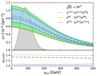
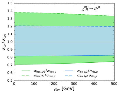
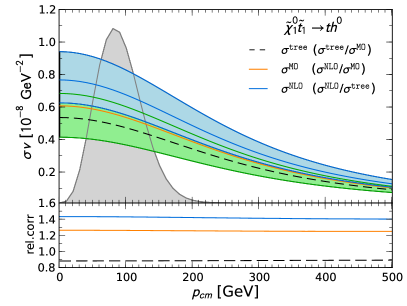
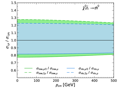
Figure 8: Cross sections of neutralino-stop coannihilation into a top quark and a light neutral Higgs boson as a function of the center-of-mass momentum $p_{\rm cm}$ in scenario C. The left plots show the annihilation cross sections calculated at the tree-level (black dashed lines) and at the one-loop level (blue solid lines) including the corresponding uncertainties from variations of the renormalization scale $\mu_{R}$ by a factor of two around the central scale (green and blue shaded bands). We also indicate the values obtained with micrOMEGAs (orange solid lines). The right plots show the cross sections normalized to their values obtained with the central renormalization scale $\mu_{R}^{\rm central}=1$ TeV. The two lower plots have been obtained using the running MSSM $\overline{\rm DR}$ top-quark mass instead of the pole mass.

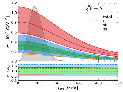
Figure 9: Cross sections of neutralino-stop coannihilation into a top quark and a light neutral Higgs boson as a function of the center-of-mass momentum $p_{\rm cm}$ in scenario C. Apart from the total cross section, we also show the contributions from the individual channels and their tree-level uncertainties induced by variations of $A_{t}$ and $A_{b}$.

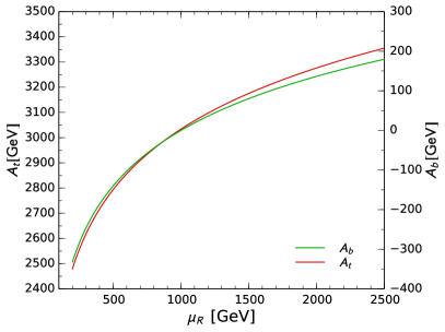
Figure 10: Dependence of the trilinear couplings $A_{t}$ (red line, left ordinate) and $A_{b}$ (green line, right ordinate) on the renormalization scale $\mu_{R}$ in scenario C.

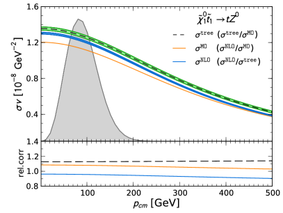
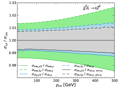
Figure 11: Cross sections of neutralino-stop coannihilation into a top quark and a $Z^{0}$ boson as a function of the center-of-mass momentum $p_{\rm cm}$ in scenario C. The left plot shows the annihilation cross section calculated at the tree-level (black dashed line) and at the one-loop level (blue solid line) including the corresponding uncertainties from variations of the renormalization scale $\mu_{R}$ by a factor of two around the central scale (green and blue shaded bands). We also indicate the values obtained with micrOMEGAs (orange solid line). The right plot shows the cross sections normalized to their values obtained with the central renormalization scale $\mu_{R}^{\rm central}=1$ TeV, at NLO also without varying the renormalization scale $\mu_{R}$ in the strong coupling constant $\alpha_{s}$ (grey shaded band).

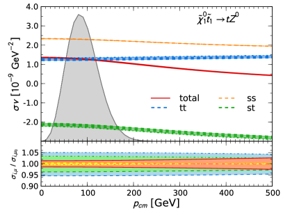
Figure 12: Cross sections of neutralino-stop coannihilation into a top quark and a $Z^{0}$ boson as a function of the center-of-mass momentum $p_{\rm cm}$ in scenario C. Apart from the total cross section, we also show the contributions from the individual channels and their tree-level uncertainties induced by variations of $A_{t}$ and $A_{b}$.

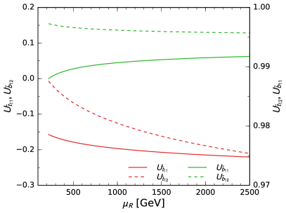
Figure 13: Dependence of the top and bottom squark mixing matrix elements on the renormalization scale $\mu_{R}$ in scenario C.

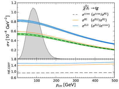
Figure 14: Same as Fig. 11, but for neutralino-stop coannihilation into a top quark and a gluon in scenario C.

When the lightest neutralino and the lightest stop are almost degenerate in mass, neutralino-stop coannihilation can contribute dominantly to the total annihilation cross section $\sigma_{\rm ann}$. Besides leading then to the correct experimentally determined value of the relic density, light stop scenarios are also well motivated by a Higgs mass of $125.09\pm 0.21\mathrm{(stat.)}\pm 0.11\mathrm{(syst.)}~{}$GeV Aad:2015zhl (cf. our discussion in Ref. Harz:2012fz ) as well as by electroweak baryogenesis Delepine:1996vn . Since neutralino-stop coannihilation processes show a different dependence on the renormalization scale from the processes discussed above, particularly in the case of a top quark and a gluon in the final state, a dedicated analysis of this situation is in order.

In the following analysis, we focus on a benchmark scenario that has already been discussed in Ref. Harz:2014tma . It involves all processes for which we provide SUSY-QCD corrections and is thus exemplary. In particular, it features important contributions of neutralino-stop coannihilation into a top quark and a gluon ($23\%$) or a Higgs boson ($23\%$), but also of neutralino pair annihilation into top quarks ($16\%$) as well as stop-antistop annihilation ($10\%$) into electroweak final states. The full list of (co)annihilation channels is given in Tab. 3. Now that the Sommerfeld enhancement and the full one-loop corrections for stop-antistop annihilation are available Harz:2014gaa , we can extend our study of this scenario in terms of the total correction to the relic density and its scale dependence. Distinctive for this scenario are low neutralino and stop masses of $338.3$ GeV and $376.3$ GeV, respectively, with a small mass difference of only $38$ GeV. This allows not only for neutralino-stop coannihilation, but also for stop-stop annihilation processes. This specific mass configuration, as well as the dominance of the top-Higgs final state, is in particular triggered by the closeness of $M_{1}$ and $M_{\tilde{u}_{3}}$ as well as a large trilinear coupling $A_{t}$. Further key features of this scenario can be found in Tabs. 1 and 2.

First, we focus on one of the two leading processes, $\tilde{\chi}_{1}^{0}\tilde{t}_{1}\to th^{0}$, for which we show the absolute cross sections as a function of the center-of-mass momentum $p_{\rm cm}$ in the upper left plot of Fig. 8. A distinct shift between the leading-order result calculated with micrOMEGAs (orange solid line) and our tree-level calculation (black dashed line) is clearly visible. This difference is again caused by different treatments of the top-quark mass. Whereas we use the pole (on-shell) mass $m_{t}^{\mathrm{OS}}$ throughout our calculation, micrOMEGAs uses an an effective top-quark mass

$$m_{\mathrm{eff}}^{2} (\mu_{R})~{}=~{}m_{t}^{2}(\mu_{R})\biggr{[}1+5.67a+\big{(}35.94-1.36n_{f}\big{)}a^{2}$$

$$+\Big{[}164.14-n_{f}\big{(}25.77-0.259n_{f}\big{)}\Big{]}a^{3}\biggr{]}$$ (10)

with $a=\alpha_{s}(\mu_{R})/\pi$, defined according to the SLHAplus library Belanger:2010st . $m_{t}(\mu_{R})$ and $\alpha_{s}(\mu_{R})$ are the running top-quark mass and strong coupling constant in the SM $\overline{\mathrm{MS}}$ scheme, respectively. As long as $\mu_{R}>2m_{t}^{\rm OS}=348.2$ GeV, this effective mass is used for calculations in micrOMEGAs. Since the scale is fixed at $\mu_{R}=2m_{\chi_{1}^{0}}=676.6$ GeV in micrOMEGAs, $m_{\rm eff}$ is therefore used there in our scenario C.

For further insight, we change in the lower left plot of Fig. 8 our usual on-shell top-quark mass $m_{t}^{\rm OS}$ to the MSSM $\overline{\mathrm{DR}}$ mass $m_{t}^{\overline{\rm DR}}$, that is also easily available in our code and that is much closer to the SM $\overline{\rm MS}$ mass than the pole mass. This corresponds to a change of the renormalization scheme, which should in principle be discussed at the same level as changes of the renormalization scale. As expected, the two tree-level calculations differ then much less than before. In addition, the micrOMEGAs tree-level calculation lies between our leading-order calculation and our NLO results as expected, since the effective top mass in Eq. (10) includes higher-order corrections to the SM $\overline{\mathrm{MS}}$ top mass. While in the upper left plot of Fig. 8 the micrOMEGAs result lies outside our tree-level uncertainty (green shaded) band, it falls within it and approaches our NLO uncertainty (blue shaded) band after the adjustment of our top quark mass in the lower left plot. When comparing the upper- and lower-left tree-level (green shaded) uncertainty bands, we notice a significant reduction when we use $m_{t}^{\overline{\rm DR}}$, which is induced by a now complementary scale dependence in the running top quark mass and stop mixing angle. The impact of the different definition of the top-quark mass is particularly enhanced due to the large trilinear coupling $A_{t}$ in scenario C and a dominant contribution of the $t$-channel diagram, see Fig. 9, which depends directly on the top mass through the squark-squark-Higgs coupling. Nevertheless, we stick to our choice of an on-shell top mass in the following, as it better fits our supersymmetric processes and on-shell top-quark final states. As one can see from the NLO scale uncertainty (blue shaded) bands, which do (hardly) overlap in the upper (lower) left plots, as well as from two left lower subplots, this choice leads to enhanced perturbative stability and a reduction of the $K$-factor from 1.4 to less than 1.1.

With the pole mass, the scale dependence is reduced from about $\pm 30\%$ at LO to about $\pm 20\%$ at NLO, as one can see in the upper right plot of Fig. 8. At LO, the scale dependence is mainly induced by the large trilinear coupling with a total scale dependence of about $15\%$ as shown in Fig. 10. This dependence is reduced at NLO due to cancellations between the vertex corrections to the squark-squark-Higgs coupling and the corresponding contributions in the renormalization group equation (RGE) of $A_{t}$. The scale dependence of $\alpha_{s}$, that enters first at NLO, is of minor importance.

Fig. 9 shows a detailed breakdown of the tree-level processes $\tilde{\chi}_{1}^{0}\tilde{t}_{1}\to th$, obtained with variations of $\mu_{R}$ in the trilinear coupling $A_{t}$. It is dominated by the highly scale-dependent $t$-channel, which induces most of the LO scale dependence in Fig. 8. In contrast, the $s$-channel shows almost no scale dependence. As this channel gains in importance for a larger center-of-mass momentum, the overall scale dependence diminishes for larger $p_{cm}$, as visible in Fig. 8. Note that the true scale uncertainty of our calculation is likely to be smaller than just explained. This is due to the fact that we take the value of $A_{t}(\mu_{R})$ directly from SPheno, which includes scale-dependent electroweak loop contributions. These are of course not cancelled by our SUSY-QCD NLO calculation.

Second, we study in Fig. 11 the process $\tilde{\chi}_{1}^{0}\tilde{t}_{1}\to tZ^{0}$. With 5%, it contributes subdominantly to the relic density in scenario C, but it is nevertheless theoretically interesting, as it shows a much smaller scale dependence than the process with a Higgs final state. The left plot in Fig. 11 shows again a distinct difference between the two tree-level calculations. In the case of a $Z^{0}$ boson in the final state, these differences arise now mostly from differently defined squark mixing angles and the dependent mass of the heavier stop Harz:2012fz . Our NLO calculation results in a correction of about $5\%$ with respect to our tree-level calculation and of about $10\%$ in comparison to micrOMEGAs, as the lower left subplot shows.

The right plot of Fig. 11 exhibits more clearly the relative scale dependence of our LO and NLO calculations. Whereas the former increases with $p_{\rm cm}$ from $\pm 1.5\%$ to $\pm 2.5\%$, it always stays below $\pm 1.5\%$ at NLO. The grey shaded band has been obtained without varying $\mu_{R}$ in $\alpha_{s}$. As one can see, the implicit scale dependence induced at NLO by the strong coupling constant is again negligible compared to the loop corrections reducing the scale dependence of the trilinear coupling.

The increase of the scale dependence with $p_{cm}$ can be understood from Fig. 12. It shows that the $t$-channel process contributes dominantly to the scale dependence, as both couplings and the propagator contain scale-dependent parameters, i.e. the squark mixing matrices and the stop mass $m_{\tilde{t}_{2}}$. As for higher $p_{cm}$ the stop mass in the propagator is less important, the scale dependence decreases. In contrast, the $s$-channel contains only the relatively light top-quark propagator and a single source of scale dependence in the neutralino-stop-top coupling. Overall, it is as important as the $t$-channel, but less scale dependent. Its scale dependence increases with $p_{\rm cm}$ due to the interplay between the mixing angles (see Fig. 13), and this translates into a slightly increased scale dependence of the total cross section at larger $p_{cm}$.

The scale dependence of the two neutralino-stop coannihilation processes discussed so far was large with about $\pm 20\%$ at NLO for Higgs final states and very small for the $Z^{0}$-boson final state with around $\pm 1.5\%$. In both cases a reduction was visible from LO to NLO despite the fact that these were purely electroweak processes at tree level. As a third coannihilation process, we now consider the semi-weak process $\tilde{\chi}_{1}^{0}\tilde{t}_{1}\to tg$, which contributes again with 23% to the relic density in scenario C. As one can see in the left plot of Fig. 14, the micrOMEGAs and our tree-level calculations differ in this case by less than 10%. However, our NLO corrections induce a relatively large $K$-factor of more than 1.5. The right plot in Fig. 14 shows that the LO scale uncertainty, induced mainly by the presence of $\alpha_{s}(\mu_{R})$ already at this order, is smaller than $\pm 4\%$. This is due to the fact that $\mu_{R}=0.5...2$ TeV is already quite large and the running of $\alpha_{s}$ relatively slow (cf. Fig. 2). The scale dependence is reduced by the NLO corrections as expected to a level of $\pm 2\%$.

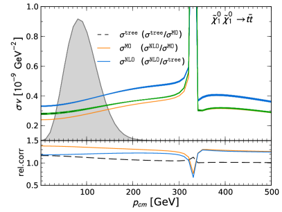
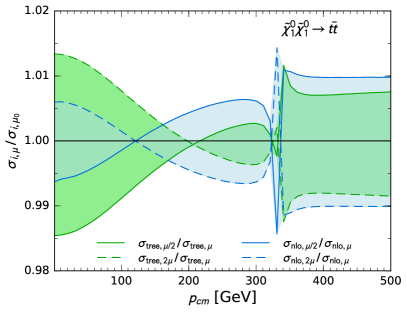
Figure 15: Same as Fig. 11, but for neutralino annihilation into a pair of top quarks in scenario C.

The third most important process in scenario C contributing 16% to the relic density is the pair annihilation of two neutralinos into a top-antitop pair, $\tilde{\chi}^{0}_{1}\tilde{\chi}^{0}_{1}\to t\bar{t}$. This is again a purely electroweak process at LO and is similar to the processes discussed for scenario A in Sec. III.1. In the left plot of Fig. 15 we show the annihilation cross section of this channel as a function of the center-of-mass momentum $p_{\rm cm}$. It exhibits a peak at $p_{\rm cm}\simeq 330$ GeV from the heavy neutral Higgs resonances, that lies however far beyond the peak of the thermal dark matter velocity distribution. At and below this peak, the micrOMEGAs and our tree-level calculations differ again visibly due to the different mass and mixing angle definitions, but agree rather well at high energy. The NLO $K$-factor is about 1.25 except at the resonance.

The dependence on the renormalization scale is, however, less important in this case, as can be seen from the right plot of Fig. 15. Varying the renormalization scale between $\mu_{R}=0.5$ and $\mu_{R}=2$ TeV leads to a variation of the LO cross section of less than two percent. Since the top-quark mass is treated in the on-shell scheme (see Sec. II), it is independent of the scale. Furthermore, the scale-dependent trilinear coupling does not enter the calculation at the tree-level, since the lightest neutralino is a pure bino. We have verified numerically that the scale-dependence of the heavier stop mass does not influence the cross section in a visible way. The only relevant scale-dependent parameter is thus the stop mixing angle $\theta_{\tilde{t}}$, which is relevant for the squark exchange in $t$- and $u$-channel diagrams. The latter dominate the cross section, except for the $s$-channel resonance of heavy Higgs bosons around $p_{\rm cm}\approx 330$ GeV. The observed dependence on the scale can thus be attributed to the variation of the stop mixing angle shown in Fig. 13.

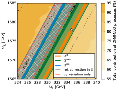
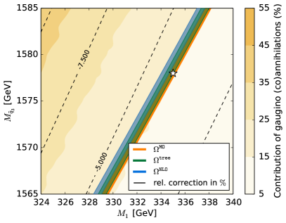
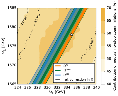
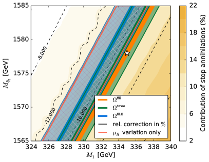
Figure 16: Cosmologically preferred regions with respect to Eq. (1) in the $M_{1}$-$M_{\tilde{q}_{3}}$-plane surrounding scenario C (white star). The solid bands correspond to the limits of Eq. (1), while the shaded bands include an additional variation of the renormalization scale $\mu_{R}$ between $\mu_{R}^{\rm central}/2$ and $2\mu_{R}^{\rm central}$. The shades of yellow indicate the percentages of the total and individual annihilation cross sections which have been corrected in our calculation, while the dashed lines represent contours of the relative correction to the relic density in percent.

Let us now turn to the discussion of the neutralino relic density, which we show in Fig. 16 in the $M_{1}$-$M_{\tilde{q}_{3}}$-plane surrounding scenario C using the same color code as before. The three bands correspond to that part of the parameter space, which leads to a relic density compatible with the Planck limits of Eq. (1) when using the micrOMEGAs effective tree level (orange), our tree level (green) and our full $\mathcal{O}(\alpha_{s})$ calculation (blue). The two last ones are surrounded by green and blue shaded bands, which illustrate the scale uncertainty obtained by varying both $\mu_{R}$ and $\mu_{C}$ by factors of two. The red shaded bands correspond to varying only $\mu_{R}$. The yellow background contours denote the relative contribution of processes we have implemented at NLO.

We start our discussion with the upper left plot, where we have used all our subprojects in parallel. The total contribution of DM@NLO processes amounts to 85-90% in the region of the three bands. This means that our code is able to improve on almost all the relevant processes in the selected part of the parameter space. As expected from our previous work, the three central predictions clearly separate. The impact of the radiative corrections on the resulting relic density is much larger than the experimental uncertainty given by Planck. More precisely, we observe a remarkable relative shift of our full result in comparison to micrOMEGAs for the relic density of 27%. This is indicated by the black dashed lines in Fig. 16. Furthermore we observe rather large theoretical uncertainty bands. Within the scale uncertainty, our tree level result agrees with micrOMEGAs and our full result, but our full result does not agree with micrOMEGAs. Moreover, the scale dependence of the full result is smaller than the scale dependence of our tree level as expected after our detailed discussion above. The impact of varying $\mu_{C}$ is subdominant in this case, i.e. the blue shaded and red hashed bands almost agree. We return to this point when discussing the lower right plot of Fig. 16.

It is quite illustrative to compare this plot with the right plot of Fig. 11 in Ref. Harz:2014tma , which shows the same part of the parameter space. In comparison, we have increased the contribution of our subprocesses from 78 to 88%, enhanced the corrections to the relic density from 18 to 27% and thus increased the shift of the compatible relic density band. This is mainly due to the fact that stop annihilation into electroweak final states is now available. In the following, we decompose the upper left plot of Fig. 16 into those pertinent to the individual subprocess contributions in order to analyze the origin of their scale dependence.

In the upper right plot, we have corrected only the gaugino (co)annihilation processes, i.e. in particular $\tilde{\chi}^{0}_{1}\tilde{\chi}^{0}_{1}\rightarrow t\bar{t}$, which contributes 16% to the relic density (see Tab. 3). Its relative contribution is also illustrated by the shades of yellow and increases to more than 35% in the direction of the upper left corner in the $M_{1}$-$M_{\tilde{q}_{3}}$-plane. This is precisely the direction of a bigger mass gap between the lightest neutralino and the lightest stop, where stop annihilation becomes irrelevant and neutralino-stop coannihilation less relevant. The three uncertainty bands overlap and show almost no dependence on the scale. Still the relative shift of the relic density amounts to 4 to 5%, even though in scenario C gaugino (co)annihilation is of minor importance compared to the other subprocesses. If we increase its contribution, i.e. look at the upper left corner of the plot, this process causes a relative shift of more than 10% when contributing 35%, which is quite remarkable for neutralino annihilation (compare with e.g. Ref. Herrmann:2014kma ). This is of course due to the large correction of the corresponding cross section (see Fig. 15 and the associated discussion). We remind the reader that SUSY-QCD corrections for neutralino annihilation into heavy quarks are particularly relevant, when there is no small mass splitting between neutralinos and stops Herrmann:2007ku ; Herrmann:2009wk ; Herrmann:2009mp .

The lower left plot shows the impact of neutralino-stop coannihilation. Together, these processes contribute more than 60% and cause a relative shift of the relic density of 14%. The scale dependence is similar to the upper left plot. Within its scale uncertainty our tree level agrees with micrOMEGAs and our full result, but our full result differs from micrOMEGAs. This is in agreement with our discussion of the contributing cross sections (cf. Figs. 8, 11 and 14). Remember that in particular the process $\tilde{\chi}^{0}_{1}\tilde{t}_{1}\rightarrow th^{0}$ featured a large scale dependence caused by its dependence on the trilinear coupling $A_{t}$. As this process contributes 23% to the relic density, the relic density also shows a rather large scale dependence. Furthermore, the scale dependence of the relic density decreases at NLO, as it is the case for all the discussed cross sections.

The remaining, lower right plot shows the impact of stop annihilation. It contributes roughly 10% in the region of the three bands and becomes more important in the direction of the lower right corner of the $M_{1}$-$M_{\tilde{q}_{3}}$-plane, the direction of a smaller mass gap between the lightest neutralino and the lightest stop. Hence the shades of yellow are complementary to the contours for gaugino (co)annihilation shown directly above. The relative shift of the relic density amounts to roughly 15%, which is very large for a subprocess contributing only 10%. It is caused by the large radiative corrections on the cross sections induced by Sommerfeld enhancement. Nevertheless, these corrections seem to be surprisingly large compared to our previous work Harz:2014gaa and the previous subsection. This has the following reason. Remember that the Sommerfeld enhancement becomes relevant for small relative velocities of the incoming particles. On the other hand, when calculating the relic density, the cross sections are weighted with the thermal distribution of these particles. In scenario C we have rather light neutralinos and stops (338.3 GeV and 376.3 GeV, cf. Tab. 2), which let the thermal distribution peak below $p_{\mathrm{cm}}\sim 100$ GeV (cf. Fig. 11). In scenario B the particles were much heavier (1306.3 GeV and 1361.7 GeV, cf. Tab. 2), and the thermal distribution peaked above $p_{\mathrm{cm}}\sim 250$ GeV (cf. Fig. 4). This means that the low-velocity tail of the cross section, where the Sommerfeld enhancement really matters, gets now a bigger weight than in scenario B Harz:2014gaa , and hence the Sommerfeld enhancement affects the relic density even more drastically. We also observe rather broad uncertainty bands for our tree-level and full results. The first one is mainly triggered by the dependence of the tree level on the trilinear coupling $A_{t}$. The second one is caused by the remaining dependence on $A_{t}$ and the dependence of the SUSY-QCD corrections on $\alpha_{s}$. This is in agreement with the findings of the previos subsection. However, in comparison to the previous subsection we also find a difference. The impact of varying $\mu_{C}$ is smaller than before, i.e. the red and blue shaded bands almost agree. This is due to the fact that $A_{t}$ constitutes the dominant source of scale dependence in this scenario. Note that varying $A_{t}$ between 0.5 and 2 TeV leads to a change of $\sim 15$% in this scenario (cf. Fig. 10) instead of $\sim 3$% in scenario B (cf. Fig. 5). This leads to a much broader tree-level uncertainty than before, and the green shaded band in the lower right plot of Fig. 16 is larger than in Fig. 7. When taking into account all subprocesses in parallel as in the upper left plot of Fig. 16, the impact of $\mu_{C}$ is further reduced, since the gaugino (co)annihilation and neutralino-stop coanniliation processes depend only on $\mu_{R}$.

An extraction of the pMSSM-11 parameters from the Planck relic density with micrOMEGAs would lead to $M_{1}=335\pm 0.5$ GeV and $M_{\tilde{u}_{3}}=1578\pm 1$ GeV and a precision of about 1 per mille, while our calculations would rather imply $M_{1}=330\pm 2$ GeV and $M_{\tilde{u}_{3}}=1578\pm 4$ GeV, i.e. a shift in $M_{1}$ by 5 GeV or 1.5% with an uncertainty of $0.5\%$, five times bigger than naively believed.

IV Conclusion

In summary, we have presented in this paper the first estimate of the theoretical uncertainty of the SUSY dark matter relic density from renormalization scheme and scale variations. Using three typical benchmark scenarios of a pMSSM with eleven free parameters, we have analyzed in particular gaugino (co)annihilation into heavy quarks, gaugino-stop coannihilation into top quarks and electroweak gauge and Higgs bosons or gluons, and stop-antistop annihilation processes. Due to different renormalization schemes in particular in the top quark sector, we have obtained results that differ from standard dark matter programs such as micrOMEGAs already at the tree level. We have quantified the impact of the renormalization scheme in this context in particular for neutralino-stop coannihilation into top quarks and the lightest, SM-like Higgs boson. We have also explained in detail how a renormalization scale dependence enters all calculations already at tree level through coupling constants, in particular the trilinear coupling $A_{t}$ for electroweak or the strong coupling $\alpha_{s}$ for strong processes, through the running bottom quark mass, in particular in the resonant Higgs funnel, and through the scale-dependent squark mixing angles in $t$- and $u$-channel squark-exchange processes.

Depending on the considered subprocesses and their relative importance for the calculation of the total relic density, the renormalization scale dependence can differ significantly, but it is reduced in almost all cases when NLO SUSY-QCD corrections are included. This was true despite the fact that $\alpha_{s}$ enters often for the first time at that order and could be traced to a slow, subdominant running of the strong coupling at the high scales of ${\cal O}$ (1 TeV) considered here. For neutralino-stop coannihilation into top quarks and Higgs bosons we could demonstrate an enhanced perturbative stability of our mixed renormalization scheme over a $\overline{\rm DR}$ definition of the top quark mass with a significantly reduced $K$-factor and scale dependence.

As in our previous work, the stop-antistop annihilation channel showed the largest corrections due to Sommerfeld enhancement at the cosmologically important low relative stop velocities. The resummation of potential gluon exchanges introduced an additional dependence on the Coulomb scale, which we chose to lie close to the Bohr radius of the would-be stoponium. The scale uncertainty was then of similar order (about $\pm 20\%$) as in the perturbative region despite the fact that the correction could amount to factors of 10 in the low-velocity regime.

The net effect of our calculations is that the relic density cannot always be determined theoretically with a precision of two percent similar to the experimental one (cf. Eq. (1)). Higher-order SUSY-QCD corrections rather induce important shifts of up to 50% as we observed in our second benchmark scenario with important Sommerfeld enhancement effects in stop-antistop annihilation (cf. Fig. 7). The theoretical uncertainty could now be more reliably estimated to be about six times as large as the experimental one. In our first benchmark scenario, dominated by gaugino (co)annihilation, the relic density corrections reached only up to 10%, and the NLO theory uncertainty became comparable to the experimental one (cf. Fig. 3). An intermediate case with important neutralino-stop coannihilation and additional other contributions was presented in our third scenario (cf. Fig. 16). There the relic density corrections reached almost 30% and the theoretical uncertainty was reduced by almost a factor of two from LO to NLO, but it remained about six times larger than the experimental one. If one wanted to extract the pMSSM parameters from the relic density measurement, one would consequently have to contend with shifts and uncertainties at the few percent rather than the per mille level in these parameters, that one would naively extract from standard contour plots.

In this paper, we have of course only studied SUSY-QCD effects and ignored scheme and scale uncertainties from the electroweak sector. While they are implicitly present to some extent in the renormalization group running of our physical parameters, we leave their explicit study for future work.

- (1) F. Zwicky, Helv. Phys. Acta 6, 110 (1933).
- (2) M. Klasen, M. Pohl and G. Sigl, Prog. Part. Nucl. Phys. 85, 1 (2015).
- (3) P. A. R. Ade et al. [Planck Collaboration], arXiv:1502.01589 [astro-ph.CO].
- (4) C. L. Bennett et al. [WMAP Collaboration], Astrophys. J. Suppl. 208, 20 (2013).
- (5) P. Gondolo and G. Gelmini, Nucl. Phys. B 360, 145 (1991).
- (6) K. Griest and D. Seckel, Phys. Rev. D 43, 3191 (1991).
- (7) J. Edsjö and P. Gondolo, Phys. Rev. D 56, 1879 (1997).
- (8) J. Harz, B. Herrmann, M. Klasen, K. Kovarik and Q. L. Boulc’h, Phys. Rev. D 87, 054031 (2013).
- (9) J. Harz, B. Herrmann, M. Klasen, K. Kovarik and M. Meinecke, Phys. Rev. D 91, 034012 (2015).
- (10) N. Baro, F. Boudjema and A. Semenov, Phys. Lett. B 660, 550 (2008); N. Baro, F. Boudjema, G. Chalons and S. Hao, Phys. Rev. D 81, 015005 (2010); F. Boudjema, G. Drieu La Rochelle and S. Kulkarni, Phys. Rev. D 84, 116001 (2011); F. Boudjema, G. D. La Rochelle and A. Mariano, Phys. Rev. D 89, 115020 (2014).
- (11) T. Bringmann and F. Calore, Phys. Rev. Lett. 112, 071301 (2014); T. Bringmann, A. J. Galea and P. Walia, Phys. Rev. D 93, 043529 (2016)
- (12) M. Beneke, C. Hellmann and P. Ruiz-Femenia, JHEP 1303, 148 (2013) [JHEP 1310, 224 (2013)]; C. Hellmann and P. Ruiz-Femenía, JHEP 1308, 084 (2013); M. Beneke, F. Dighera and A. Hryczuk, JHEP 1410, 45 (2014); M. Beneke, C. Hellmann and P. Ruiz-Femenia, JHEP 1505, 115 (2015); M. Beneke, C. Hellmann and P. Ruiz-Femenia, JHEP 1503, 162 (2015); M. Beneke, A. Bharucha, F. Dighera, C. Hellmann, A. Hryczuk, S. Recksiegel and P. Ruiz-Femenia, arXiv:1601.04718 [hep-ph].
- (13) J. Hisano, K. Ishiwata and N. Nagata, JHEP 1506, 097 (2015).
- (14) M. Drees, J. M. Kim and K. I. Nagao, Phys. Rev. D 81, 105004 (2010); A. Chatterjee, M. Drees and S. Kulkarni, Phys. Rev. D 86, 105025 (2012); M. Drees and J. Gu, Phys. Rev. D 87, 063524 (2013).
- (15) B. Herrmann and M. Klasen, Phys. Rev. D 76, 117704 (2007).
- (16) B. Herrmann, M. Klasen and K. Kovarik, Phys. Rev. D 79, 061701 (2009).
- (17) B. Herrmann, M. Klasen and K. Kovarik, Phys. Rev. D 80, 085025 (2009).
- (18) B. Herrmann, M. Klasen, K. Kovarik, M. Meinecke and P. Steppeler, Phys. Rev. D 89, 114012 (2014).
- (19) J. Harz, B. Herrmann, M. Klasen and K. Kovarik, Phys. Rev. D 91, 034028 (2015).
- (20) J. A. Aguilar-Saavedra et al., Eur. Phys. J. C 46, 43 (2006).
- (21) W. Porod, Comput. Phys. Commun. 153, 275 (2003); W. Porod and F. Staub, Comput. Phys. Commun. 183, 2458 (2012).
- (22) G. Belanger, S. Kraml and A. Pukhov, Phys. Rev. D 72, 015003 (2005).
- (23) Y. Kiyo, J. H. Kühn, S. Moch, M. Steinhauser and P. Uwer, Eur. Phys. J. C 60, 375 (2009).
- (24) M. Beneke, PoS HF 8, 009 (1999).
- (25) M. Beneke, P. Falgari and C. Schwinn, Nucl. Phys. B 842, 414 (2011).
- (26) M. Beneke, Y. Kiyo and K. Schuller, Nucl. Phys. B 714, 67 (2005).
- (27) G. Belanger, F. Boudjema, A. Pukhov and A. Semenov, Comput. Phys. Commun. 149 103 (2002); G. Belanger, F. Boudjema, A. Pukhov and A. Semenov, Comput. Phys. Commun. 177 894 (2007).
- (28) A. Pukhov, hep-ph/0412191. A. Belyaev, N. D. Christensen and A. Pukhov, Comput. Phys. Commun. 184, 1729 (2013).
- (29) G. Aad et al. [ATLAS and CMS Collaborations], Phys. Rev. Lett. 114, 191803 (2015).
- (30) D. Delepine, J. M. Gerard, R. Gonzalez Felipe and J. Weyers, Phys. Lett. B 386, 183 (1996).
- (31) G. Belanger, N. D. Christensen, A. Pukhov and A. Semenov, Comput. Phys. Commun. 182, 763 (2011).
- (32) J. D. Hunter, Computing In Science & Engineering 9, 90 (2007).