Magnetic moments in a helical edge can make weak correlations seem strong

Abstract

We study the effect of localized magnetic moments on the conductance of a helical edge. Interaction with a local moment is an effective backscattering mechanism for the edge electrons. We evaluate the resulting differential conductance as a function of temperature $T$ and applied bias $V$ for any value of $V/T$. Backscattering off magnetic moments, combined with the weak repulsion between the edge electrons results in a power-law temperature and voltage dependence of the conductance; the corresponding small positive exponent is indicative of insulating behavior. Local moments may naturally appear due to charge disorder in a narrow-gap semiconductor. Our results provide an alternative interpretation of the recent experiment by Li et al. Li et al. (2015) where a power-law suppression of the conductance was attributed to strong electron repulsion within the edge, with the value of Luttinger liquid parameter $K$ fine-tuned close to $1/4$.

Introduction - In search for topological insulators, the III-V semiconductor structures with band inversion appeared as a viable option Liu et al. (2008). The band inversion does occur in the type-2 heterostructure, InAs/GaSb. If the layers forming the well are narrow enough, the hybridization of states across the interface results in a formation of a gap; in the “topological” phase, the gap is accompanied by edge states free from elastic backscattering. These putative states became a target of an extensive set of measurements Knez et al. (2014); Spanton et al. (2014); Du et al. (2015); Li et al. (2015); Nichele et al. (2015). First, a surprisingly robust conductance quantization was found Du et al. (2015). A later experiment Li et al. (2015) explained the temperature-independent quantized conductance $G$ as an inadvertent deviation from the linear-response regime. The observed Li et al. (2015) power-law temperature and bias voltage dependence of the differential conductance was suggestive of insulating behavior. Assuming topologically protected edge states, it can be interpreted as a manifestation of strong-interaction physics: at low energies, even a single impurity can “cut” the edge, suppressing charge transport Kane and Fisher (1992) if the Luttinger parameter is very small, $K<1/4$ Wu et al. (2006); Xu and Moore (2006) ($K=1$ corresponds to non-interacting electrons). Measurements Li et al. (2015) yield $K\approx 0.22$ (with a 5% error), which is very close to the critical value of $1/4$; an increase of $K$ by mere 12% would change the sign of $dG/dT$. Fine-tuning $K$ to such a stable value seems improbable, given the dependence of the edge state velocity on the gate voltages, varied in the experiment. The reliance on fine-tuning in the current explanation of experiments provides an impetus to search for alternatives less sensitive to a specific value of $K$.

We find that scattering off localized magnetic moments may lead to temperature and bias dependences of the differential conductance similar to those observed Li et al. (2015) at moderately weak interaction, $K\approx 0.8$, without fine-tuning of $K$. The origin of localized moments in InAs/GaSb quantum wells is not known, but the narrow 40-60K gap in these systems may allow for the presence of charge puddles Väyrynen et al. (2013) which can act as magnetic impurities Väyrynen et al. (2014). In the present work we focus on the non-linear current-voltage characteristics and on the effects of electron-electron interactions within the helical edge which were not considered in Ref. Väyrynen et al. (2014).

The setup and qualitative description of the main results - We start by considering a single spin-1/2 magnetic moment $\mathbf{S}$ coupled to a helical edge. The isolated edge is described Wu et al. (2006) by a Luttinger liquid Hamiltonian $H_{0}$; the local moment is coupled to the edge electrons by, generally, anisotropic exchange interaction. Separating out its isotropic part, the full time-reversal symmetric Hamiltonian of the coupled edge-impurity system can be written as

$$H=H_{\text{iso}}+\sum_{ij}\delta J_{ij}S_{i}s_{j}(x_{0})$$ (1)

with $H_{\text{iso}}$ being the Hamiltonian with isotropic exchange:

$$H_{\text{iso}}=H_{0}+J_{0}\mathbf{S}\cdot\mathbf{s}(x_{0})$$ (2)

Here, $\mathbf{S}$ is the spin-1/2 impurity spin operator, and $\mathbf{s}(x_{0})=\frac{1}{2}\sum_{\alpha\beta}\psi_{\alpha}^{\dagger}(x_{0})\boldsymbol{\sigma}_{\alpha\beta}\psi_{\beta}(x_{0})$ is the edge electron spin density at the position $x_{0}$ of the contact interaction with the local moment. (From hereon we will omit the position arguments.) We shall assume $\delta J_{ij}\ll J_{0}$ so that the exchange is almost isotropic Väyrynen et al. (2014). Thus we can treat the second term in Eq. (1) as a perturbation.

The first term in $H_{\text{iso}}$, Eq. (2) is the bosonized Luttinger-liquid Hamiltonian describing the interacting helical edge electrons, $H_{0}=(2\pi)^{-1}v\int dx[\Pi^{2}+(\partial_{x}\varphi)^{2}]$; we assume the dimensionless exchange coupling parameter to be small, $\rho J_{0}\ll 1$ (here $\rho$ is the electron density of states per spin per unit edge length). The bosonic fields commute as $[\varphi(x),\Pi(y)]=i\pi\delta(x-y)$. We have rescaled the fields by appropriate factors of $\sqrt{K}$; the bosonization identity is $\psi_{\beta}(x)=(2\pi a)^{-1/2}e^{-i(\beta\sqrt{K}\varphi-\frac{1}{\sqrt{K}}\int_{-\infty}^{x}dx^{\prime}\Pi)}$ with $\beta=+/-$ for right/left movers (or spin up/down; we take $\mathbf{z}$-axis to be the spin quantization axis of helical electrons at Fermi energy); $a$ is the short-distance cutoff. In bosonic representation, the spin density takes form $s_{x}\pm is_{y}=\pm i(2\pi a)^{-1}e^{\pm 2i\sqrt{K}\varphi}$, $s_{z}=\frac{1}{2\pi\sqrt{K}}\Pi$. Using it, we re-write the exchange interaction Hamiltonian as

$$\!J_{0}\mathbf{S}\cdot\mathbf{s}\!\to\!J_{\perp}\frac{-i}{4\pi a}(S_{+}e^{-2i\sqrt{K}\varphi}-S_{-}e^{2i\sqrt{K}\varphi})+J_{z}\frac{1}{2\pi\sqrt{K}}S_{z}\Pi\,.$$ (3)

Even though the bare Hamiltonian (2) is isotropic, $J_{\perp}=J_{z}=J_{0}$, the exchange becomes anisotropic under renormalization group (RG) flow, as the scaling dimensions of the corresponding spin densities in Eq. (3), $\Delta_{\perp}=K$ and $\Delta_{z}=1$, differ from each other Sénéchal (2004), see also Eqs.(4)–(5) below. The isotropy breaking is not an artefact: anisotropy is already present in the bare Hamiltonian even at $K=1$ due to the spin-orbit interaction; the Hamiltonian has no SU(2) symmetry but only a smaller U(1) symmetry (spin rotations about $z$-axis).

The weak-coupling ($\rho J\ll 1$ and $1-K\ll 1$) RG equations for $J_{\perp}$ and $J_{z}$ are Lee and Toner (1992); Furusaki and Nagaosa (1994); Maciejko et al. (2009) (here $E$ is the running cutoff)

$$\frac{dJ_{\perp}}{d\ln E} =-(1-K)J_{\perp}-\rho J_{z}J_{\perp}$$ (4)

$$\frac{dJ_{z}}{d\ln E} =-\rho J_{\perp}^{2}$$ (5)

The right-hand-side of the first equation starts at tree level with a coefficient Cardy (1996); Sénéchal (2004) $1-\Delta_{\perp}=1-K$; the second equation does not have such a term since $\Delta_{z}=1$. The terms second-order in $J$ are due to the Kondo effect and can be derived from poor man scaling Anderson (1970), or from an operator product expansion Cardy (1996); Sénéchal (2004).

Starting from isotropic initial condition, $J_{0}>0$, Eq. (4) shows that there are two regimes of parameters: $\rho J_{0}\ll 1-K$ and $\rho J_{0}\gg 1-K$. In the latter case $1-K$ can be dropped from Eq. (4), and the physics is similar to that of the case $K=1$ Väyrynen et al. (2014).

In this paper we focus on the opposite limit, $\rho J_{0}\ll 1-K$. (Note, such initial condition can be satisfied even if the electron-electron interaction is weak, $1-K\ll 1$.) In this case the RG flow governed by Eqs. (4)–(5) can be divided into two regimes separated by energy scale $T^{*}$ (we use units $k_{B}=\hbar=1$) defined by the crossover condition Giamarchi (2003) $\rho J_{z}(T^{*})=1-K$,

$$T^{*}=D(\frac{1}{\sqrt{2}}\frac{\rho J_{0}}{1-K})^{1/(1-K)}\,.$$ (6)

Here $D\sim E_{g}$ is the bare cutoff which we take to be the bulk band gap . At energies $E\gg T^{*}$ one can ignore $\rho J_{z}(E)$ in (4), whereas at $E\ll T^{*}$ one can ignore $1-K$. Next, we discuss electron backscattering in the high energy limit, $E\gg T^{*}$ where interaction ($K\neq 1$) is important.

The backscattering current at energies above $T^{*}$ -The isotropic exchange Hamiltonian (2) alone does not backscatter edge electrons in steady state (DC bias) since each backscattering event is accompanied by an action of the nilpotent operator $S_{-}$ on the impurity spin polarized along $\mathbf{z}$-axis Tanaka et al. (2011). The presence of anisotropy in the exchange, Eq. (1), gives rise to backscattering. This perturbation in Eq. (1) can be treated using Fermi Golden Rule, assuming equilibrium impurity polarization $\left\langle\mathbf{S}\right\rangle=\mathbf{z}\frac{1}{2}\tanh\frac{eV}{2T}$ . Integration over electron phase space volume leads to a backscattering current $\left\langle\delta I\right\rangle\sim e^{2}V(\rho\delta J)^{2}$. We can find the full temperature and bias voltage dependence by solving for the renormalized coupling $\delta J$. Since the pertinent constant $\delta J$ couples to the spin-flip operators $e^{\pm 2i\sqrt{K}\varphi}$, it acquires a power-law energy dependence $\delta J(E)=(D/E)^{1-K}\delta J(D)$ for $E>T^{*}$. Taking $E\sim\max(T,\,eV)$, the $T$ and $V$ -dependent backscattering current becomes (valid at $\max(T,\,eV)\gg T^{*}$)

$$\left\langle\delta I\right\rangle=\frac{e^{2}}{h}cV\,T^{-2(1-K)}[\max(1,\,eV/T)]^{-2(1-K)}\,,$$ (7)

where constant $c$ depends on the bare exchange tensor. Equation (7) is a simplified version of our main result. Its detailed version, see Eq. (14), reveals, in addition to $eV/T\sim 1$, yet another crossover in the current-voltage characteristic occurring at $\frac{eV}{T}\sim\rho J\ll 1$; it is associated with the details of impurity spin torque and relaxation, ignored in Eq. (7).

Long edge conductance at energies above $T^{*}$ - Let us now consider a long sample which may host many impurities near the edge. A single impurity contributes an amount $\delta R\approx\delta G/G_{0}^{2}$to the edge resistance (here $G_{0}=e^{2}/h$ and $\delta G=d\left\langle\delta I\right\rangle/dV$). In a long sample with $N$ impurities we can simply add resistances if the impurities are dilute enough . The impurities dominate the edge resistance if $N\delta G\gg G_{0}$, where the same typical value $\delta G$ for each impurity is used. In this case one finds $G\approx G_{0}^{2}/N\delta G$ for the conductance of a single edge. Here $\delta G$ is evaluated with the help of Eq. (14) or its simplified version, Eq. (7), both valid at $\max(T,\,eV)>T^{*}$.

Using Eq. (7) one finds a power-law dependence $G(V,T)\approx(G_{0}/cN)[\max(T,\,eV)]^{2(1-K)}$. In Ref. Li et al. (2015) the authors found a fit $G\propto V^{0.37}$ in the regime $eV>T$ for a sample of length $L=1.2\mu\text{m}$ (see inset in Fig. 4 of Ref. Li et al. (2015)). Matching with our theory of many impurities leads to $2(1-K)\approx 0.37$, or $K\approx 0.82$. Thus, in presence of many impurities, even moderately weak interactions can give rise to the power law seen in Ref. Li et al. (2015). The two possible explanations (many impurities and weak interaction vs. single impurity and strong interaction) of the observed conductance predict different dependencies of $G$ on the edge length: for many impurities one expects $N\propto L$ and hence resistive behavior $G\propto L^{-1}$. Although $G(L)$ dependence is not reported in Ref. Li et al. (2015), the earlier work Du et al. (2015) found it to be linear at $L\gtrsim 10\mu{\rm m}$  . The presence of magnetic impurities may also be identified from their subtle effect on the non-linear $I$-$V$ characteristics, which we discuss next.

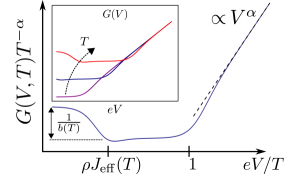
Figure 1: (Color online) Log-log plot of the scaled conductance, $G\cdot T^{-\alpha}$, in the presence of many impurities, $G\propto 1/\delta G$. Here $\delta G=d\left\langle\delta I\right\rangle/dV$ and $\alpha=2-2K>0$ are taken from Eq. (14), valid at intermediate energies $\max(T,eV)>T^{*}$. The conductance has two crossover scales in its $V$-dependence. The higher crossover is at $eV\sim T$: above it, conductance increases (upon increasing $V$) asymptotically as a power law with exponent $\alpha>0$ (dashed line). Below it, $G$ stays roughly constant until the lower crossover scale, $eV\sim\rho J_{\text{eff}}(T)T$, is reached. Below it, the conductance changes by a factor $1/b(T)>1$ that depends weakly on temperature, see discussion below Eq. (16). The inset shows $G(V)$ at three different temperatures $T$ (increasing from the lowest to highest curve).

Refinement of Eq. (7) - The simplified form Eq. (7) of the current-voltage characteristic misses several fine points relevant for the future analysis of experiments: (1) it does not provide the accurate form of the crossover at $eV/T\sim 1$, and (2) it does not reveal an additional crossover at smaller bias, $eV/T\sim\rho J$. The latter crossover is associated with the precession of the local magnetic moment in the exchange field $h\sim eV\rho J$ produced by the spins of itinerant edge electrons under a finite bias Note (2). The crossover occurs once the precession frequency $\propto h$ becomes comparable to the Korringa relaxation rate, Korringa (1950) $1/\tau_{K}\sim(\rho J)^{2}T$, as we will see in a detailed derivation of backscattering current.

The current operator of backscattered electrons is given by Kane and Fisher (1994) $\delta I=-e\partial_{t}\delta N$ where $2\delta N=(N_{L}-N_{R})$ is the difference between the number of left and right movers on the edge; it obeys $[\delta N,\,s_{i}(x_{0})]=i\epsilon_{zin}s_{n}(x_{0})$ and commutes with $H_{0}$. The decomposition (1) of the Hamiltonian is useful because at zero frequency the Hamiltonian $H_{\text{iso}}$, Eq. (2), does not lead to backscattering of helical edge electrons Tanaka et al. (2011). It can be seen by noticing that: (i) $\partial_{t}\left\langle S_{z}\right\rangle=0$ in a steady state, because $S_{z}$ is bounded; this allows one to write the average backscattering current as Väyrynen et al. (2014) $\left\langle\delta I\right\rangle=-e\partial_{t}\left\langle S_{z}^{tot}\right\rangle$ with $S_{z}^{tot}=\delta N+S_{z}$, and (ii) the operator $S_{z}^{tot}$ commutes with $H_{\text{iso}}$ and therefore is a conserved quantity in absence of $\delta J_{ij}$. Hence $\partial_{t}\left\langle S_{z}^{tot}\right\rangle|_{\delta J\to 0}=0$ and $\left\langle\delta I\right\rangle|_{\delta J\to 0}=0$. We focus here on the case of a single magnetic moment; in the presence of many moments, we can define $S_{z}^{tot}=\delta N+\sum_{n}S^{(n)}_{z}$ where the sum is over the localized spins $\mathbf{S}^{(n)}$. In this work, we ignore the effects of correlations between the localized spins and coherent backscattering, allowing us to simply add up single-moment contributions to the edge resistance. This is justified for dilute spins, as discussed in more detail in Ref. Note (3).

From hereon, we consider scattering off a single spin, and express the average steady-state backscattered current as $\left\langle\delta I\right\rangle=-e\partial_{t}\left\langle S_{z}^{tot}\right\rangle$. Commuting with the Hamiltonian (1) leads to [we denote $\delta J_{++}=\delta J_{xx}-\delta J_{yy}+i{(\delta J_{xy}+\delta J_{yx})},\,S_{\pm}=S_{x}\pm iS_{y}$ for brevity]

$$\left\langle\delta I\right\rangle=e\sum_{i,j=x,y}\epsilon_{ijz}\left(\delta J_{jz}\left\langle S_{i}:s_{z}:\right\rangle+\delta J_{zj}\left\langle S_{z}:s_{i}:\right\rangle\right)$$ (8)

$$\!+e\text{Im}\delta J_{++}\left\langle S_{-}:\!s_{-}:\right\rangle+\!\frac{1}{2}\rho e^{2}V\left(\delta J_{yz}\left\langle S_{x}\right\rangle-\delta J_{xz}\left\langle S_{y}\right\rangle\right)\,.$$

In agreement with the presence of an integral of motion, the average current vanishes when $\delta J\to 0$. The averaging above is done with respect to the density matrix $\varrho$ with Hamiltonian (1) in presence of a finite bias voltage, $\varrho\sim e^{-\beta\left(H-eVS_{z}^{tot}\right)}$ Väyrynen et al. (2014). We denote $:\!s_{j}\!:=s_{j}-\langle s_{j}\rangle_{0}$ with $\langle\rangle_{0}$ being the thermal average in absence of exchange interaction, $\varrho_{0}\sim e^{-\beta\left(H_{0}-eV\delta N\right)}$. The last term in (8) comes from the reducible part $\langle s_{j}\rangle_{0}=\frac{1}{2}\delta_{jz}\rho eV$.

Equation (8) is evaluated at time $t$ long enough so that the steady-state value of $\left\langle\mathbf{S}\right\rangle$ has been reached. The averages $\langle S_{k}\!:\!s_{l}\!:\rangle$ can be evaluated approximately in the exchange interaction assuming a separation of time scales for the itinerant electron and spin dynamics Note (3). The approximation results in

$$\langle S_{k}:\negthinspace s_{l}\negthinspace:\rangle(t) \approx-\sum_{j}(\delta_{kj}J_{0}+\delta J_{kj})\frac{1}{2}\text{Im}C_{jl}$$ (9)

$$-\sum_{ijn}(\delta_{ij}J_{0}+\delta J_{ij})\epsilon_{ikn}\left\langle S_{n}\right\rangle\text{Re}C_{jl}\,.$$

Here $\left\langle S_{n}\right\rangle$ is the steady-state impurity spin polarization created by the current passing on the edge. The integrated correlation function $C_{nl}=\int_{0}^{\infty}dt^{\prime}\left\langle s_{n}(0)\!:\!s_{l}(t^{\prime})\!:\right\rangle_{0}$ depends on temperature and bias voltage (through the average $\langle\dots\rangle_{0}$). The only non-zero components of the matrix of $C_{nl}$ are the diagonals and $C_{xy}\!=\!-C_{yx}\neq 0$, the latter being due to finite bias voltage. The temperature and bias dependence of $C_{nl}$ appearing in Eq. (9) can be moved into the $T$ and $V$ dependence of running couplings $J_{ij}(T,V)$ Note (3). Inserting Eq. (9) into Eq. (8) allows us to express the backscattering current in terms of the running couplings and steady-state values of the local-moment spin polarization $\left\langle\mathbf{S}\right\rangle$, see Ref. Note (3). The last is found from the Bloch equations Bloch (1946). At $\delta J=0$, its only finite component is $\left\langle S_{z}\right\rangle=\frac{1}{2}\tanh\frac{eV}{2T}$ due to the $U(1)$ symmetry. Aiming at the lowest-order in $\delta J$ result for $\langle\delta I\rangle$, we need to find $\left\langle S_{x,y}\right\rangle$ to the first order in $\delta J$. Unlike $\left\langle S_{z}\right\rangle$, which is a function of $eV/T$ given by thermodynamics, the components $\left\langle S_{x,y}\right\rangle$ depend Note (3) on both the effective field $h_{z}=\frac{1}{2}eV\rho J_{z}$ generated by the bias voltage, and on the local-moment Korringa relaxation rate $\tau_{K}^{-1}=\frac{\pi}{2}\rho^{2}(J_{\perp}^{2}\frac{\frac{eV}{2T}}{\tanh\frac{eV}{2T}}+J_{z}^{2})T$. (We use here the running couplings with their implicit dependence on $V$ and $T$.) The backscattering current is

$$\left\langle\delta I\right\rangle =e\frac{\pi}{4}eV\rho^{2}|\delta J_{++}(T,V)|^{2}+e\frac{\pi}{4}eV\frac{1}{2}R(T,V)$$ (10)

$$\times\sum_{i=x,y}\rho^{2}\left(\delta J_{zi}(T,V)+\frac{J_{\perp}(T,V)}{J_{z}(T,V)}\delta J_{iz}(T,V)\right)^{\!2}\!.$$

Here the first term arises from non-zero $\left\langle S_{z}\right\rangle$ and can be derived simply from Fermi Golden Rule by assuming $\left\langle\mathbf{S}\right\rangle=\mathbf{z}\frac{1}{2}\tanh\frac{eV}{2T}$. In the second term, function

$$R(T,V)\approx\frac{\frac{J_{z}(T,0)}{J_{\text{eff}}(T)}+x^{2}}{1+x^{2}}\,,\quad x=\frac{eV}{2T}\frac{2/\pi}{\rho J_{\text{eff}}(T)}\,,$$ (11)

comes from $\left\langle S_{x,y}\right\rangle\neq 0$ and therefore depends on the ratio $h_{z}/\tau_{K}=x$. Here we abbreviated $\rho J_{\text{eff}}(T)=\rho{[J_{\perp}(T,0)^{2}+J_{z}(T,0)^{2}]}/J_{z}(T,0)\ll 1$. In Eq. (11) the term $J_{z}/J_{\text{eff}}\lesssim 1$ only matters at very small bias $eV\ll T\rho J_{\text{eff}}\ll T$; thus we have neglected the $V$-dependence in it.

In Eq. (10) the current is written in terms of the running couplings $J_{ij}(T,\,V)$. Next, we will write it in terms of the bare couplings, which allows us to see explicitly the $T,V$-dependence of $\left\langle\delta I\right\rangle$. At $T^{*}<\max(eV,\,T)<D$ one has Note (3)

$$X(T,V)\approx X(D)\left(\frac{D}{2\pi T}\right)^{1-K}\sqrt{F(\frac{eV}{2T})}$$ (12)

with a function

$$F(y)=KB(K+i\frac{y}{\pi},K-i\frac{y}{\pi})\frac{\sinh y}{y}\approx\frac{B(K,K)}{[1+A(K)y^{2}]^{1-K}}\,.$$ (13)

Here $A(K)=\pi^{-2}\Gamma(K)^{\frac{2}{1-K}}$ and $B$ is the Euler Beta function; $X$ stands for any of the quantities, $\text{Re}\delta J_{++},\,\text{Im}\delta J_{++},$ and $\delta J_{zi}+\frac{J_{\perp}}{J_{z}}\delta J_{iz}$ ($i=x,\,y$), which appear in Eq. (10).

Using Eqs. (10)–(13) we arrive at the central result of this paper: the temperature and bias dependence of the current can be lumped in a product of several simple terms,

$$\left\langle\delta I\right\rangle=\delta G_{0}\left[\frac{D}{2\pi T}\right]^{2-2K}V\frac{B(K,K)}{[1+A(K)(\frac{eV}{2T})^{2}]^{1-K}}f(x,T)\,,$$

$$f(x,T)=\frac{b(T)+x^{2}}{1+x^{2}}\,,\,\,x=\frac{eV}{2T}\frac{2/\pi}{\rho J_{\text{eff}}(T)}.$$ (14)

Here the $T$-independent factor is $\delta G_{0}=\frac{e^{2}}{\hbar}\frac{\pi}{4}\rho^{2}\delta J_{\text{tot}}^{2}(D)\,,$

$$\delta J_{\text{tot}}^{2}(D)\negthinspace=|\delta J_{++}(D)|^{2}+\frac{1}{2}\sum_{i=x,y}[\delta J_{zi}(D)+\delta J_{iz}(D)]^{2}\,,$$ (15)

while $J_{\text{eff}}(T)$ and

$$b(T)\negthinspace=1-\frac{(1-\frac{J_{z}(T,0)}{J_{\text{eff}}(T)})\frac{1}{2}\sum_{i=x,y}[\delta J_{zi}(D)+\delta J_{iz}(D)]^{2}}{|\delta J_{++}(D)|^{2}+\frac{1}{2}\sum_{i=x,y}[\delta J_{zi}(D)+\delta J_{iz}(D)]^{2}}\,$$ (16)

display a weak temperature dependence Note (3). (For typical values of exchange couplings $\delta J_{ij}(D)$ function $b(T)$ can be well approximated by a constant of order 1: $0.67\leq b(T)\leq 0.83$ in the interval $T^{*}\leq T\leq D$ Note (3).) At a fixed temperature $T$, the current dependence on bias $V$ has two well-separated crossover scales described by the last two factors in (14). The smaller scale, $V\sim T\rho J_{\text{eff}}(T)$, is associated with the impurity spin dynamics. The crossover at the higher scale, $V\sim T$, occurs between the linear and weakly-nonlinear $\langle\delta I\rangle$ vs. $V$ dependencies. Near this crossover one may set $f\to 1$ in Eq. (14), reproducing the result of Eq. (7) with, however, accurate crossover behavior near $eV\sim T$.

The backscattering current at energies below $T^{*}$ - At energies $E\lesssim T^{*}$, one may neglect the small term $\propto(1-K)$ in (4)–(5) and consider the resulting weak-coupling Kondo RG with the initial condition $\rho J_{\perp}(T^{*})=\sqrt{2}(1-K)$ Note (3). For small $1-K$, it yields the Kondo temperature $T_{K}\sim T^{*}e^{-1/\sqrt{2}(1-K)}\ll T^{*}$. The RG flow erases the uniaxial anisotropy created by $K\neq 1$, and $J_{z}\approx J_{\perp}$ at energies below $T^{*}$. As a result, $J_{\text{eff}}=2J_{z}$ in Eq. (11) and $R=(\frac{1}{2}+x^{2})/(1+x^{2})$. Similarly, the anisotropic perturbation in Eq. (1) becomes RG-irrelevant, and Eq. (12) is replaced Väyrynen et al. (2014) by $X(E)\approx X(T^{*})\frac{\ln E/T_{K}}{\ln T^{*}/T_{K}}$. Hence, the backscattering current becomes

$$\left\langle\delta I\right\rangle=\delta G_{0}V\left[\frac{\ln\max(T,eV)/T_{K}}{\ln T^{*}/T_{K}}\right]^{2}\frac{b+x^{2}}{1+x^{2}}\,,$$ (17)

valid for $T_{K}<\max(T,eV)<T^{*}$. Here $b$ is given by Eq. (16) which becomes independent of $T$ upon setting $J_{\text{eff}}=2J_{z}$. Similarly, $\delta G_{0}$ was introduced below Eq. (14) but now one must use $\delta J_{\text{tot}}^{2}(T^{*})$ in it with the “new” bare cutoff.

The coupling constant $\rho J_{z}(E)\sim[\ln(E/T_{K})]^{-1}$ grows in the course of RG, and below the Kondo temperature, $\max(T,eV)<T_{K}$, Eqs. (4)–(5) are no longer valid. In this regime one can use the phenomenological local-interaction Hamiltonian Schmidt et al. (2012); Lezmy et al. (2012) to obtain $\delta G(V,T)\propto T^{4}g(V/T)$; the crossover function $g(x)$ has asymptotes $g(x\to 0)=\rm const$ and $g(x\gg 1)\sim x^{4}$. Details can be found in Ref. Lezmy et al. (2012) upon setting $K=1$ therein. Note that $\delta G$ decreases when reducing $T,\,eV$ and thus leads to $G=e^{2}/h$ in the limit of zero temperature and bias. This behavior is opposite from Eq. (14) which indicated an insulating edge at low energies.

Conclusions - We analyzed the joint effect of two weak interactions on the edge conduction in a 2D topological insulator. These interactions are: the repulsion between itinerant electrons of an edge state, and their exchange with the local magnetic moments. This joint effect may result in a seemingly insulating behavior of the edge conduction down to a low temperature scale $T^{*}$, see Eq. (6): at $\max(T,eV)\gtrsim T^{*}$, the single-impurity backscattering current $\left\langle\delta I\right\rangle$ grows as a power law upon lowering temperature or bias, see Eq. (14), or Fig. 1 for the conductance in presence of many moments. Localized magnetic moments may appear in a narrow-gap semiconductor as a consequence of charge disorder Väyrynen et al. (2014). Scattering off magnetic moments provides an alternative explanation of the recent experiment Li et al. (2015), assuming $T^{*}$ is below the temperature range explored in Li et al. (2015). [None of the considered interactions break the time-reversal symmetry , so at low energies, $\max(T,eV)\ll T^{*}$, backscattering is suppressed, see Eq. (17).] The developed theory is also applicable to magnetically-doped Jungwirth et al. (2006)  heterostructures. Finally, we find two crossovers in the $I$-$V$ characteristics: the main one occurs at $eV\sim T$; a more subtle one occurs at lower bias, $eV\sim\rho JT$, see Fig. 1. Its observation in future experiments may provide evidence for the considered mechanism of the edge state excess resistance.

in 1,…,8 See pages \x of Supplement.pdf