Luminosity function of luminous compact star-forming galaxies

Abstract

We study H$\alpha$, far- and near-ultraviolet luminosity functions (LF) of the sample of 795 luminous compact star-forming galaxies with $z<0.65$. The parameters of optimal functions for LFs are obtained using the maximum likelihood method and the accuracy of fitting is estimated with the $\chi^{2}$ method. We find that these LFs cannot be reproduced by the Schechter function because of an excess of very luminous galaxies. On the other hand, the Saunders function, the log-normal distribution and some new related functions are good approximations of LFs. The fact that LFs are not reproduced by the Schechter function can be explained by the propagating star formation. This may result in an excess of luminous starbursts with the mass of a young stellar population above $2\times 10^{8}$ M_⊙ as compared to the LF of the quiescent galaxies. The most luminous compact galaxies are characterised by H$\alpha$ luminosities of $\geq 5\times 10^{42}$ erg s^-1 and star formation rates of $\geq 40$ M_⊙ yr^-1.

Keywords Galaxies: luminosity function, mass function — Galaxies: starburst — Galaxies: star formation

1 Introduction

We study the luminosity functions (LFs) of the sample of 795 luminous compact galaxies (LCG) for the H$\alpha$ emission line, far ultraviolet (FUV) and near ultraviolet (NUV) continua. Recent bursts of star formation with age less than 6 Myr are present in all galaxies as evidenced by very high H$\beta$ emission-line equivalent widths. Thus, our sample consists of extreme compact galaxies, populating the high-end tail of the LF of the overall star-forming population.

In this paper we consider five functions to fit the LFs of our sample, namely the Schechter function (Schechter, 1976), the Saunders distribution (Saunders et al., 1990), the log-normal one and two functions proposed by Parnovsky (2015). The Schechter function was commonly used to approximate LFs in the H$\alpha$ emission line and ultraviolet (UV) range. However, it was argued in some recent papers that observed LFs deviate from the Schechter function due to an excess of very luminous galaxies. Gunawardhana et al. (2013) found that the H$\alpha$ LF for Galaxy And Mass Assembly (GAMA) galaxies with $z<0.35$ is better described by the Saunders function, which can be reduced to the log-normal distribution for the considered sample.

The H$\alpha$ and UV radiation is produced by the population of massive stars, which were formed during the recent burst. Therefore, galaxy luminosities at these wavelengths attain a maximum shortly after a starburst. Later on, the H$\alpha$ and UV luminosities strongly decrease with time after a starburst age $T_{0}\approx 3.2$ Myr, when the most massive stars start to fade out. The temporal dependence of this rapid luminosity evolution was found by Parnovsky et al. (2013). It has a form

$$L(T)=L_{0}f(T),\,\,f(0)=1,$$ (1)

where $T$ is the starburst age, $L_{0}$ is the luminosity at $T=0$, and $f(T)$ is approximated by

$$f(T)=\left\{\begin{array}[]{rl}1&\textrm{if $T\leq T_{0}$;}\\ \exp(-p(T-T_{0}))&\textrm{if $T>T_{0}$,}\\ \end{array}\right.$$ (2)

with $T_{0}=3.2$ Myr and the exponent $p$, which depends on the wavelength (see details in Parnovsky et al., 2013; Parnovsky & Izotova, 2013). The same function is appropriate for the luminosities in the 22 $\mu$m IR band, derived using the Wide-field Infrared Survey Explorer (WISE) data and probably for the radio emission at 1.4 GHz (Parnovsky & Izotova, 2015).

Naturally, the rapid luminosity evolution affects the observed LF. This effect was studied by Parnovsky (2015), who derived the functional forms of LFs in the cases when the initial galaxy luminosities $L_{0}$ are approximated by the Schechter or log-normal distributions. However, we note that the decrease with time of the starburst H$\alpha$ luminosity is much steeper than that of the FUV and NUV luminosities. This is because the H$\alpha$ emission is produced only by the most massive short-lived stars while the contribution of the less massive and longer-lived stars to the FUV and NUV emission is important.

In particular, between 0 and 10 Myr it decreases by more than two orders of magnitude, while the FUV luminosity is decreased only by a factor of two (Leitherer et al., 1999). Izotov et al. (2014) have shown that the FUV-to-H$\beta$ luminosity ratio for galaxies with high EW(H$\beta$) is lower than that for galaxies with low EW(H$\beta$). This is due to the more rapid evolution of the H$\beta$ luminosity. Therefore, H$\alpha$ and FUV luminosities first should be reduced to zero age and only after that be compared.

Our goal is to find functional dependences, which provide the best fitting of the sample LFs and to derive sets of their optimal parameters. We use the methods of the mathematical statistic described e.g. by Fisher (1954) and Hudson (1964). The maximum likelihood method (MLM) is used to derive an optimal set of parameters and the Pearson’s $\chi^{2}$-test is applied to estimate the accuracy of fitting.

The properties of the sample are described in Section 2. We justify the choice of the approximations for the luminosity functions in Section 3. Luminosity functions in the H$\alpha$ emission line and UV continuum are considered in Sections 4 and 5, respectively. A brief discussion of possible physical mechanisms influencing the LF shape is presented in Section 6. The best LFs approximations are summarised in Section 7.

2 Data description

We use the sample of 795 LCGs selected by Izotov, Guseva & Thuan (2011) from the Data Release 7 of the Sloan Digital Sky Survey (SDSS)(Abazajian et al., 2009). These data were supplemented by FUV ($\lambda_{\rm eff}$= 1528Å) and NUV ($\lambda_{\rm eff}$ = 2271Å) fluxes, extracted by Parnovsky et al. (2013) from the GALEX Medium and All-sky Imaging Surveys.

Briefly, the sample selection criteria were as follows: high equivalent width EW(H$\beta$) $\geq$ 50Å and high luminosity $L$(H$\beta$) $\geq$ 3$\times$10⁴⁰ erg s^-1 of the H$\beta$ emission line; well-detected [O iii] $\lambda$4363 Å emission line in galaxy spectra, with a flux error less than 50%. Only star-forming galaxies with angular diameters $\leq 10\arcsec$ were selected. All these criteria select galaxies with strong emission lines in their spectra at redshifts $z$ $\sim$ 0.02 – 0.6. The high equivalent width EW(H$\beta$) results in selection of LCGs with starburst ages $T<5$ Myr.

Izotov et al. (2011) showed that LCGs from this sample occupy the region of star-forming galaxies with high-excitation H ii regions in the [O iii]$\lambda$5007/H$\beta$ vs. [N ii]$\lambda$6583/H$\alpha$ diagnostic diagram (BPT diagram, Baldwin, Phillips & Terlevich, 1981). All LCGs lie below the line (Kauffmann et al., 2003) separating star-forming galaxies and active galactic nuclei.

LCGs are characterised by strong and rare bursts of star formation and their properties are similar to those of so-called “green pea” (GP) galaxies discussed by Cardamone et al. (2009). These galaxies have low metallicities (of $\sim$ 20 % solar) (Amorín et al., 2010; Izotov et al., 2011), low stellar masses of $\sim 10^{8.5}$ – $10^{10}M_{\odot}$ (Cardamone et al., 2009; Izotov et al., 2011), strong [O iii] $\lambda\lambda$ 4959, 5007Å emission lines, high star formation rates (SFR $\sim 10$ M_⊙yr^-1, Cardamone et al., 2009) and high specific star formation rates (up to $\sim 10^{-8}$ yr^-1, Cardamone et al., 2009; Izotov et al., 2011). These features place them between nearby blue compact dwarf galaxies on one side and high-redshift UV-luminous Lyman-break galaxies and H$\alpha$ emitters on the other side.

Some parameters of these LCGs including the starburst ages $T$ and the masses of the young stellar population $m$ were obtained from fitting their spectral energy distributions in the wavelength range $\lambda$$\lambda$3800 – 9200Å (see details of selection criteria and derived global characteristics in Izotov et al., 2011). Neither $T$ nor $m$ were used as selection criteria.

The reddening corrections to H$\alpha$ and UV band fluxes are applied adopting the Cardelli et al. (1989) reddening law. The extinction $A(V)$ and reddening $E(B-V)$ of each galaxy was obtained by Izotov et al. (2011) from the hydrogen Balmer decrement in the rest frame SDSS spectra. Adopting $R(V)$ = $A(V)/E(B-V)$ = 3.1, we obtain $A$(H$\alpha$) = 2.54$\times$$E(B-V)$, $A$(FUV) = 8.15$\times$$E(B-V)$ and $A$(NUV) = 9.17$\times$$E(B-V)$. All hydrogen line fluxes were corrected for both the reddening and underlying stellar absorption.

Note that Izotov et al. (2016) checked different reddening laws comparing SDSS optical and HST/COS UV spectra of one of the compact galaxies. They found that reddening curves with low $R(V)$ $\sim$ 2.7 are more suitable, while the reddening law by Calzetti et al. (1994) and Calzetti et al. (2000) is not appropriate. All H$\alpha$ emission line luminosities were also corrected for aperture.

To verify these corrections we compared the H$\alpha$ line luminosities for LCGs with their luminosities in the 22 $\mu$m IR band, calculated using WISE data. We find that the H$\alpha$-to-22 $\mu$m band luminosity ratios for our galaxies are approximately constant, indicating that these luminosities are approximately proportional with a linear Pearson’s correlation coefficient of 90%. Similar proportionality was obtained by Lee, Hwang & Ko (2013) and Izotov et al. (2014) (see also Battisti et al., 2015). Adopting the Cardelli et al. (1989) reddening law Izotov et al. (2014) found that the FUV-to-H$\alpha$ and NUV-to-H$\alpha$ luminosity ratios are also constant. However, the exact values of the latter ratios depend on the adopted $R(V)$, while H$\alpha$-to-22 $\mu$m band luminosity ratios are not sensitive to the value of $R(V)$.

The luminosities were corrected for extinction derived individually in each galaxy. According to Salim & Lee (2012) only a sample with individual corrections for extinction can show the deviation of LF from the Schechter function. LFs without extinction correction or corrected using averaged statistical relations have a form that is similar to the Schechter function by a coincidence.

Summarising, the entire sample consists of 795 galaxies with H$\alpha$ luminosities (Parnovsky et al., 2013). The majority of these galaxies were also detected in the FUV and NUV ranges. Additionally we extracted a subsample of 691 galaxies with a single star-forming region by discarding the galaxies with multiple knots of star formation. This subsample is used to study the rapid luminosity evolution and to compare with theoretical predictions by Parnovsky (2015), which were made for the galaxies with a single star-forming region.

3 Analythical functions for fitting of the LF

3.1 Commonly used LF approximations

The luminosity function is a very important statistical characteristic of galaxy populations. The optical LF can be reproduced by the Schechter function, which is also known in the mathematical statistics as the gamma distribution:

$$\varphi(L)\propto(L/L^{*})^{\alpha}\exp(-L/L^{*}).$$ (3)

Here $\varphi(L)dL$ is the number of galaxies per unit volume in the luminosity interval from $L$ to $L+dL$. Parameters $\alpha$ and $L^{*}$ are determined from the shape of this function. The slope in the [$\ln\varphi(L),\ln L$] plane is equal to $\alpha$ for $L\ll L^{*}$ and is strongly changed at $L\approx L^{*}$.

We define the probability density of luminosity distribution $n(L)$, called the sample LF, by introducing a probability $n(L)dL$ for the galaxy, randomly selected from a sample, to have the luminosity in the interval from $L$ to $L+dL$. If $N$ is the number of galaxies in the sample then $Nn(L)dL$ is the number of galaxies with the luminosity in the interval from $L$ to $L+dL$.

To find $n(L)$ we multiply the function $\varphi(L)$ by the volume $V(L)$ occupied by the sample galaxies with the luminosity $L$. For a flux-limited sample with small galaxy redshifts we can adopt $V(L)\propto L^{3/2}$ neglecting the effect of general relativity and differences between the luminosity distance and other types of distances in relativistic cosmology. Then the sample LF is described by the relation

$$n(L)=\frac{u^{\alpha+3/2}e^{-u}}{L^{*}\Gamma(\alpha+5/2)},\quad u=\frac{L}{L^{*}}.$$ (4)

Here $\Gamma$ is the gamma-function. The constant $1/\Gamma(\alpha+5/2)$ is derived from the normalisation condition

$$\int_{0}^{\infty}n(L)dL=1.$$ (5)

The deviation of LFs from the Schechter function was noted for the far-IR (FIR) luminosities at 60 $\mu$m (Lawrence et al., 1986; Saunders et al., 1990; Takeuchi, Yoshikawa & Ishii, 2003) or radio luminosities (Condon, Cotton & Broderick, 2002; Willott et al., 2001; Machalski & Godlowski, 2000). On the other hand, until recently, it was suggested that LFs for the H$\alpha$ line (Gallego et al., 1995; Ly et al., 2011) and the UV emission (Wyder et al., 2005) can well be fitted by a Schechter function.

At the same time all these luminosities are indicators of star formation (Calzetti, 2012), therefore their extinction-corrected LFs must be similar. Since FIR and radio LFs are not described by the Schechter function, the deviation of the H$\alpha$ and UV LFs from this function is also expected. However, this deviation was found only recently. A reason is that the luminosities in H$\alpha$ line and UV ranges must be individually corrected for the dust extinction, unlike the FIR or radio luminosities. Without this correction the deviation of LF from the Schechter one is masked.

Salim & Lee (2012) showed that the Schechter function can not reproduce the distributions of SFRs derived from the UV and H$\alpha$ fluxes, and therefore their LFs are also not fitted by the Schechter function. On the other hand, optical and near-infrared LFs are well reproduced by the Schechter function. This conclusion was made on the basis of the UV SFR-to-mass ratio distribution of about 50,000 galaxies in the local universe with $z\leq 0.1$ (Salim et al., 2007).

Jurek et al. (2013) studied the UV LF of galaxies from the Galaxy Evolution Explorer (GALEX) Medium Imaging Survey with spectroscopic redshifts from the DR1 of the WiggleZ Dark Energy Survey (Drinkwater et al., 2010). They found an excess of most luminous galaxies compared to the Schechter distribution at redshifts greater than $z=0.55$.

Bowler et al. (2014) claimed that the bright end of the UV LF is declined not as steeply as that predicted by the Schechter function of fainter galaxies for the sample of 34 luminous galaxies in the redshift range $6.5<z<7.5$ from the UltraVISTA DR2 and UKIDSS UDS DR10 surveys.

Similarly Parnovsky, Izotova & Izotov (2013) found the excess of galaxies at the bright end of the H$\alpha$, FUV and NUV LFs for LCGs. In this paper we study LFs of this sample in more detail.

Gunawardhana et al. (2013) found that the H$\alpha$ LF for GAMA galaxies with $z<0.35$ is not well described by the Schechter function. The exponential drop of the Schechter function at the bright end is too steep to match the observed LFs, which are better approximated by the Saunders function (Saunders et al., 1990)

$$\begin{array}[]{c}n(L)=\textrm{const}\times u^{\beta}\exp\left[-A\log^{2}(1+u)\right],\\ u=L/L^{*}_{s},\quad A=1/(2\sigma^{2}).\end{array}$$ (6)

Here $\sigma$ and $L^{*}_{s}$ are constants. Note that Saunders et al. (1990) used the notation $L^{*}$ in (6). We add the subscript “$s$” to distinguish this quantity from the $L^{*}$ in (3). Fitting LF of our sample we find that the exact value of $L^{*}_{s}$ does not change an accuracy of a fit. Since the luminosities of the sample galaxies $L_{i}$ are much greater than $L^{*}_{s}$, the unity in the $(1+u)$ term can be dropped and Eq. (6) is transformed to the two-parametric log-normal distribution

$$n(L)=\left(\frac{a}{\pi}\right)^{1/2}\exp\left(-\frac{1}{4a}\right)\,\tilde{L}^{-1}\exp\left(-a\ln^{2}(L/\tilde{L})\right)$$

$$=\left(\frac{a}{\pi}\right)^{1/2}\exp\left(-\frac{1}{4a}\right)\,\tilde{L}^{-1}\left(\frac{L}{\tilde{L}}\right)^{-a\ln\left(L/\tilde{L}\right)}.$$ (7)

Here

$$a=A(\ln 10)^{-2},\quad\ln\tilde{L}=\ln L^{*}_{s}+\beta/(2a).$$ (8)

The set of three parameters ($L^{*}_{s},A,\beta$) can be reduced to the the set of two parameters ($\tilde{L},a$). We note that the intrinsic parameter $\tilde{L}$ is defined by the combination of $L^{*}_{s}$ and $\beta$ only if $L_{i}\gg L^{*}_{s}$.

3.2 An effect of a rapid luminosity evolution

Parnovsky (2015) studied the impact of the rapid luminosity evolution on the LF of a sample of star-forming galaxies by introducing the initial, current, time-averaged and sample LFs. He derived the relations between different types of LFs for the case of an arbitrary luminosity evolution defined by equation (1) (Parnovsky, 2015). Considering flat space and neglecting the differences between the luminosity distance and other types of distances Parnovsky (2015) obtained the sample LF in the form

$$n(L)=C\left[n_{1}(L)+qn_{2}(L)\right],$$ (9)

where the constant $C$ is derived from the normalisation condition (5). Here $n_{1}(L)$ is a sample LF if the rapid luminosity evolution is neglected, e.g. in the case of constant galaxy luminosities and $n_{2}(L)=L^{1/2}\int_{L}^{\infty}x^{-3/2}n_{1}(x)dx$ is the term that takes into account rapid luminosity evolution. The constant $q$ is the combination of the parameters from (2)

$$q=(T_{0}p)^{-1}.$$ (10)

It can be considered as a free parameter and can be obtained from the best fit of the sample LF. In any case, the condition $q\geq 0$ should be satisfied. The case with $q=0$ corresponds to $n(L)=n_{1}(L)$, i.e to the LF without the luminosity evolution.

Parnovsky (2015) obtained the sample LFs for the cases with initial galaxy luminosities and $n_{1}(L)$, which are approximated by the Schechter function (4) and the log-normal distribution (3.1). In the first case

$$n(L)=\frac{u^{\alpha+3/2}e^{-u}+qu^{1/2}\Gamma(\alpha+1,u)}{L^{*}(1+2q/3)\Gamma(\alpha+5/2)},u=\frac{L}{L^{*}}.$$ (11)

This relation includes the incomplete gamma-function, (see e.g. Bateman & Erdélyi, 1953)

$$\Gamma(\alpha+1,u)=\int_{u}^{\infty}x^{\alpha}e^{-x}dx$$ (12)

and depends on three parameters $q$, $\alpha$ and $L^{*}$.

In the second case

$$n(L)= \tilde{L}^{-1}\left(1+\frac{2q}{3}\right)^{-1}\times$$

$$\times\left[\left(\frac{a}{\pi}\right)^{1/2}\exp\left(-\frac{1}{4a}\right)\exp\left(-a\ln^{2}(L/\tilde{L})\right)+\right.$$

$$+\frac{q}{2}\exp\left(-\frac{3}{16a}\right)\left(\frac{L}{\tilde{L}}\right)^{1/2}\times$$

$$\left.\times\textrm{erfc}\left(\sqrt{a}\ln\left(\frac{L}{\tilde{L}}\right)+\frac{1}{4\sqrt{a}}\right)\right].$$ (13)

Here

$$\textrm{erfc}(x)=1-\textrm{erf}(x)=\frac{2}{\sqrt{\pi}}\int_{x}^{\infty}e^{-t^{2}}dt.$$ (14)

It also depends on three parameters $q$, $a$ and $\tilde{L}$.

The relations (11) and (3.2) at $q=0$ are transformed to the Schechter function (4) and the log-normal distribution (3.1), respectively. The properties of relations (11) and (3.2) were analyzed by Parnovsky (2015).

4 Approximation of the H$\alpha$ LF for the LCG sample

Using MLM and functions (4), (3.1), (6), (11) and (3.2) we derive optimal sets of parameters of the H$\alpha$ LF for the sample of LCGs. The accuracy of the fits is verified with the Pearson’s $\chi^{2}$-test.

4.1 Fitting the LF by Schechter function

We find a set of parameters $\alpha,L^{*}$, for which the function

$$U=\sum_{i=1}^{N}\log(n(L_{i}|\alpha,L^{*}))$$ (15)

with $n(L_{i}|\alpha,L^{*})$ from Eq. (4) attains a maximum. Here $L_{i}$ are the extinction- and aperture-corrected luminosities of individual galaxies from the entire sample.

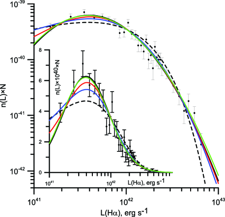
Fig. 1 : The H$\alpha$ LF of the entire LCG sample and its approximation by the log-normal distribution (3.1) (solid black line) and Schechter function (4) (dashed line). Red, blue and green lines show the functions (3.2,10), (4.5) and (6) with optimal parameters. Error bars correspond to the Poisson distribution. The smaller inner frame shows the same plot with linear ordinate axis to emphasize the differences between the approximations near their maximum. The differences at the high-luminosity end are best seen in the main plot

The maximum of Eq. (15) is attained if

$$\ln(2.5+\alpha)-\psi(2.5+\alpha)=\ln\left<L\right>-\left<\ln L\right>,$$ (16)

$$L^{*}=\frac{\left<L\right>}{2.5+\alpha}.$$ (17)

Here $\psi$ is the digamma function or the logarithmic derivative of the gamma function, and angle brackets mean the averaging over the sample. These maximum conditions are well known and were used e.g. by Kudrya et al. (1997) and Efstathiou, Ellis & Peterson (1988).

For the entire LCG sample from (16, 17) we derive $\alpha=-1.04$, $L^{*}=8.5\times 10^{41}$ erg s^-1. The Schechter distribution with these parameters predicts the mean number of galaxies entering in 9 bins with width $5\times 10^{41}$ erg s^-1 to be 203, 205, 145, 94.5, 59, 36, 21.6, 12.8, 7.5, respectively, and 10.4 galaxies with luminosities greater than $4.5\times 10^{42}$ erg s^-1. The respective number of galaxies from the observed LF is 227, 218, 139, 66, 56, 28, 17, 11, 6, 27. The excess of the most luminous galaxies is obvious. The Schechter approximation is shown in Fig. 1 by a dashed line. The similar LF excess is present for the galaxies with a single knot of star formation approximated by the Schechter function with parameters $\alpha=-0.96$, $L^{*}=8.0\times 10^{41}$ erg s^-1. We derive $\chi^{2}$ values of 42.2 and 38.9 for the entire sample and the subsample of galaxies with a single knot of star formation, respectively. The probabilities that LFs for these samples are reproduced by the Schechter function are $1.7\times 10^{-7}$ and $7.5\times 10^{-7}$ i.e. negligible.

According to Salim & Lee (2012), the individual corrections for extinction are necessary to establish the deviation of LF from the Schechter function. The similar conclusions were drawn by Gunawardhana et al. (2013). To verify the effect of the correction for extinction we consider the “uncorrected” H$\alpha$ LF for LCGs without any correction. This LF is approximated by the Schechter function with parameters $\alpha=-1.08$, $L^{*}=3.4\times 10^{41}$ erg s^-1. The predicted mean number and actual number (in parentheses) entering in 8 bins with width $2.5\times 10^{41}$ erg s^-1 are 270(307), 228(224), 137(123), 76(54), 41(34), 21(24), 11(8), 5.5(9), respectively, and 5.6(12) galaxies with luminosities greater than $2\times 10^{42}$ erg s^-1. The corresponding value of $\chi^{2}$ is 24.4, which is roughly a half of the $\chi^{2}$ value for the sample with the luminosities, corrected for extinction.

It is clear that the correction for extinction with a mean extinction for all galaxies would result in the $L^{*}$ increased by the corresponding factor, while the values of $\alpha$ and $\chi^{2}$ remain the same. Thus, the individual corrections for extinction considerably increase the $\chi^{2}$ value in agreement with the statement of Salim & Lee (2012). Nevertheless, the value of $\chi^{2}$ for the deviation of the “uncorrected” LF from the Schechter function is big enough. For 6 degrees of freedom it corresponds to the probability $\approx 0.04\%$ that LF is defined by the Schechter distribution. This difference arises because of an excess of galaxies on the bright end of LF and a deficit of galaxies in the middle region $7.5\times 10^{41}$ erg s${}^{-1}<L<10^{42}$ erg s^-1.

Thus, we can reject the possibility that sample LF is described by the Schechter function. Moreover, the LF deviates from the Schechter function even without individual luminosity correction.

4.2 Fitting the LF by log-normal function

The MLM optimal parameters for the distribution (3.1) are

$$\begin{array}[]{c}\ln\tilde{L}=\langle\ln L\rangle+\langle\ln L\rangle^{2}-\langle\ln^{2}L\rangle,\\ a=\left[2\left(\langle\ln^{2}L\rangle-\langle\ln L\rangle^{2}\right)\right]^{-1}.\end{array}$$ (18)

Angle brackets mean the averaging over the sample.

The log-normal distribution is more intuitive, it has no unnecessary parameters and its parameters can be easily obtained from Eq. (18). The distribution (3.1) is normalized according to (5). Note that the distribution of the probability density over $\ln L$ achieves the maximum at $\tilde{L}_{1}=\exp\langle\ln L\rangle$, not at $\tilde{L}$.

For the H$\alpha$ LF of the entire LCG sample we derive $a=0.657$, $\tilde{L}=3.96\times 10^{41}$ erg s^-1 and $\tilde{L}_{1}=8.5\times 10^{41}$ erg s^-1. This approximation is shown in Fig. 1 by solid black line. The $\chi^{2}$-test provides the probability 27% that deviations are random with the value $\chi^{2}=8.7$ and 7 degrees of freedom (d.o.f.). Similarly, for the subsample with a single knot of the star formation we obtain a fit with $a=0.689$, $\tilde{L}=4.12\times 10^{41}$ erg s^-1 and $\tilde{L}_{1}=8.5\times 10^{41}$ erg s^-1. Its $\chi^{2}=10.2$ corresponds to 18% probability that the difference in LFs is due to the random deviations.

4.3 Fitting the LF by Saunders function

Calculating the optimal set of parameters for Saunders function (6) using MLM, we meet with the asymptotic degeneration, when the different sets of $\beta$, $L^{*}$ and $A$ correspond to the distribution (3.1) with the same parameters $a$ and $\tilde{L}$. Consequently, the minimal $\chi^{2}$ for the fit of LF by the Saunders function should be less or equal to the value obtained by the log-normal fit.

Numerical calculations for the entire LCG sample show that a minimal value $\chi^{2}=7.1$ is achieved at $L^{*}_{s}=8\times 10^{39}$ erg s^-1, $\beta=4.69$ and $A=3.25$. The function (6) with this set of parameters is shown in Fig. 1 by the green line. The number of d.o.f. for $\chi^{2}$ is 6 for the three-parameter Saunders function, therefore the minimal value $\chi^{2}=7.1$ corresponds to the probability of 31% that the deviations between LF and the Saunders function (6) are due to the random errors. This means that the fit by the Saunders function is as accurate as the fit by the log-normal distribution. We will show in section 4.5 that the obtained probability is less than that for the fit by function (3.2).

For the subsample with a single knot of star formation the minimal value $\chi^{2}=9.0$ is attained with the set $L^{*}_{s}=8\times 10^{39}$ erg s^-1, $\beta=5.01$ and $A=3.43$. It corresponds to the probability of 17% that the difference between LF and the Saunders function is random.

Thus, we confirm the conclusion of Gunawardhana et al. (2013) that the Saunders function (6) is much better approximation of LF than the Schechter one. The bright end with $L>2.5\times 10^{42}$ erg s^-1 is fitted very well. We obtained nearly the same result with the log-normal function. The main contribution to the $\chi^{2}$ value is provided by the deficit of galaxies in the $2\times 10^{42}$ erg s${}^{-1}<L<2.5\times 10^{42}$ erg s^-1 bin.

4.4 LF fitting by the Schechter function in the case of rapid luminosity evolution

We approximate the luminosity function of the sample by (11) and find optimal values of its parameters using MLM. Parnovsky et al. (2013) derived $p=0.65$ Myr^-1 and $T_{0}=3.2$ Myr for the entire sample, therefore we obtain $q=0.48$ from (10). Adopting this value, we obtain the optimal MLM values $L^{*}=(8.5\pm 0.5)\times 10^{41}$ erg s^-1 and $\alpha=-0.88\pm 0.07$ at the 68% confidence level. In Fig. 2 we plot by solid lines the borders of $1\sigma$, $2\sigma$ and $3\sigma$ confidence regions of $\alpha$ and $L^{*}$. By dashed lines we also plot the borders of the $1\sigma$, $2\sigma$ and $3\sigma$ confidence regions for the subsample with a single knot of the star formation. The optimal values of parameters for this subsample are $L^{*}=(8.0\pm 0.5)\times 10^{41}$ erg s^-1 and $\alpha=-0.81\pm 0.07$. We find that the $1\sigma$ confidence regions for the entire sample and the subsample are substantially overlapped.

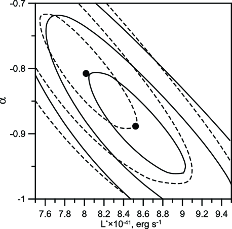
Fig. 2 : The borders of 1$\sigma$-, 2$\sigma$- and 3$\sigma$- confidence regions according to MLM. Solid and dashed lines correspond to the entire sample and the subsample of LCGs with a single knot of the star formation, respectively

Using the Pearson’s $\chi^{2}$ test we obtain $\chi^{2}=37.4$ and 33.3 with 7 d.o.f. for the entire sample and the subsample with a single knot of star formation, respectively. These values correspond to the probability less than 0.01% for the luminosity function of the samples to be of the form of Eq. (11).

The derived parameter $L^{*}$ is the same as that obtained in Section 4.1 by fitting with the Schechter function (4) and neglecting the rapid luminosity evolution. On the other hand, the values of $\alpha$ in the case of the luminosity evolution are greater by $2.3\sigma$ for the entire sample and by $2.1\sigma$ for the subsample of galaxies with a single knot of star formation than the values obtained with the Schechter function Eq. (4) . Thus, $\alpha$ is considerably underestimated if the rapid luminosity evolution is neglected.

The above conclusions are obtained for the fixed value of $q$. Now we consider the case with the varying $q$. There is the problem preventing MLM from finding the unique set of three optimal parameters considered by Parnovsky (2015). Two completely different sets of parameters are resulted in practically the same shapes of function (11). One can see in Fig. 1 from Parnovsky (2015) that the function with $\alpha=-0.51$, $L^{*}=8.08\times 10^{41}$ erg s^-1, $q=2$ is almost coincident with the function (11) and the set of parameters obtained above, namely $\alpha=-0.88$, $L^{*}=8.5\times 10^{41}$ erg s^-1, $q=0.48$. Consequently, the function $U$ from (15) has two equal maxima and a prolate form of confidence interval.

Nevertheless, varying $q$ and using MLM we search for two other parameters. For the entire sample we obtain the MLM values $\alpha=-0.77,-0.69,-0.63,-0.42,-0.39$, $L^{*}=(8.57,8.59,$ $8.63,9.16,9.70)\times 10^{41}$ erg s^-1 and $\chi^{2}=34.0,32.7,31.7,$ $27.8,27.2$ for $q=1,1.5,2,10,100$, respectively. The plots of all distributions with these sets of parameters are very similar, while parameters $\alpha$ and $L^{*}$ increase with increasing $q$. The maximum on the plot becomes slightly higher and narrower with increasing $q$. Consequently, $\chi^{2}$ is slightly decreased. The minimum of $\chi^{2}$ is attained at $q\to\infty$. The likelihood for the subsample with a single knot of star formation is maximal at $q\to\infty$ with $\alpha=-0.26$, $L^{*}=9.1\times 10^{41}$ erg s^-1, and $\chi^{2}=25.2$, corresponding to 0.14% probability that deviations of the fit from the LF are statistical.

Thus, Eq. (11) is a very poor approximation of the luminosity function of LCGs, mainly due to the excess of very luminous galaxies.

4.5 LF fitting by the log-normal function in the case of rapid luminosity evolution

To fit the LF of the entire LCG sample with the MLM we use the function (3.2) adopting $q=0.48$ and find $a=0.73$ and $\tilde{L}=4.9\times 10^{41}$ erg s^-1. The function (3.2) with this set of parameters is shown in Fig. 1 by the red line. The derived $\chi^{2}=7.6$ corresponds to 37% probability that the difference in LFs is caused by random deviations. For the subsample with a single knot of star formation we find $a=0.77$, $\tilde{L}=5.1\times 10^{41}$ erg s^-1 and $\chi^{2}=9$, corresponding to the probability of 25%.

Varying $q$ we can find the dependence of the MLM function $U$ and $\chi^{2}$ on $q$. For the subsample with a single knot of star formation $U$ decreases if $q$ increases. However, this dependence is very weak.

We give some values of $a$ and $\tilde{L}$ for different $q$. Adopting $q=0.05,0.1,1,2,5,10,30,100$ we find the values 0.70, 0.71, 0.83, 0.90, 0.98, 1.01, 1.02, 1.02 for $a$ and 4.25, 4.36, 5.87, 6.85, 8.16, 8.9, 9.4, 9.6 erg s^-1 for $\tilde{L}\times 10^{-41}$, respectively. The respective values of $\chi^{2}$ are 10.4, 9.9, 8.6, 8.5, 8.7, 8.7, 8.8, 8.8 with the minimum at $q\approx 2$. Using this value we decrease the d.o.f. by 1. The minimal value $\chi^{2}=8.5$ with 6 d.o.f. corresponds to the 20% probability that the difference between LFs is random. This probability is worse than the value obtained above with $q=0.48$ according to (10) with 7 d.o.f.

Similar conclusions can be drawn for the entire sample. Adopting $q=0.05,0.1,0.25,1,2,6,10,50,1000$ we find the values 0.668, 0.675, 0.702, 0.789, 0.854, 0.919, 0.943, 0.958, 0.959 for $a$ and 4.09, 4.18, 4.49, 5.66, 6.62, 7.99, 8.51, 9.19, 9.36 erg s^-1 for $\tilde{L}\times 10^{-41}$, respectively. The value of $U$ slightly decreases if $q$ increases. The respective values of $\chi^{2}$ are 8.65, 8.4, 8.3, 7.5, 7.5, 7.3, 7.6, 7.7, 7.7 with the minimum at $q\approx 2.5$. The difference between minimal $\chi^{2}$ and its value at $q=0.48$ according to (10) is not sufficient to compensate the reduction of d.o.f. number in attemps to increase the probability.

Summarising, there are three special values of $q$ which do not reduce the number of d.o.f. These are the limiting values $q=0$ and $q\to\infty$ and the condition (10), which is not associated with minimal $\chi^{2}$ value. We find that the function (3.2) with $q=0.48$ according to (10) provides a better fit compared to log-normal one.

The asymptotics of the function (3.2) at $q\to\infty$ has the form

$$n(L) =\frac{3}{4\tilde{L}}\exp\left(-\frac{3}{16a}\right)\left(\frac{L}{\tilde{L}}\right)^{1/2}$$

$$\times\textrm{erfc}\left(\sqrt{a}\ln\left(\frac{L}{\tilde{L}}\right)+\frac{1}{4\sqrt{a}}\right)$$

$$=\frac{3}{4L_{c}}\exp\left(-\frac{9}{16a}\right)\left(\frac{L}{L_{c}}\right)^{1/2}$$

$$\times\textrm{erfc}\left(\sqrt{a}\ln\left(\frac{L}{L_{c}}\right)\right),$$ (19)

where $L_{c}=\tilde{L}\exp(-1/4a)$. The function (4.5) has two parameters. According to MLM the best fit of the H$\alpha$ LF for the entire sample is achieved with $a=0.96$, $L_{c}=7.23\times 10^{41}$ erg s^-1 and $\tilde{L}=9.4\times 10^{41}$ erg s^-1. The function (4.5) with this set of parameters is shown in Fig. 1 by the blue line. The value $\chi^{2}=7.73$ and the 36% probability that the difference in LFs is caused by random deviations are very similar to the values obtained for the function (3.2) and the value of $q=0.48$ according to (10). The same is true also for the subsample of LCGs with a single knot of star formation. The best approximation is achieved with $a=1.02$, $L_{c}=7.6\times 10^{41}$ erg s^-1 and $\tilde{L}=9.7\times 10^{41}$ erg s^-1. The value $\chi^{2}=8.85$ corresponds to the probability of 26%.

The LF fits by functions (3.2,10) and (4.5) have similar accuracy and are better than the fit by the log-normal function.

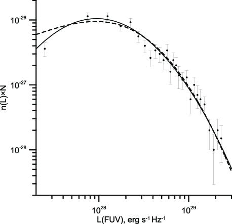
Fig. 3 : The FUV LF of the entire LCG sample and its approximation by the log-normal distribution (3.1) (solid line) and function (4.5) (dashed line). Error bars correspond to the Poisson distribution

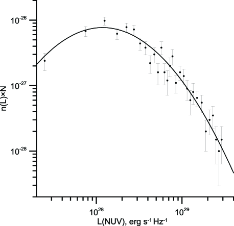
Fig. 4 : The NUV LF of the entire LCG sample and its approximation by the log-normal distribution (3.1). Error bars correspond to the Poisson distribution

4.5.1 A generalization of function (4.5)

We found that fits by (3.2) with $q$ from (10) and (4.5) are resulted in similar $\chi^{2}$ values. The advantage of the function (4.5) is that it fits the high-end of LF very well. However its behaviour at low-end is fixed and is approximated by $n(L)\propto L^{1/2}$. On the other hand, the Schechter function badly fits the high-end of LF, but its approximation at low-end LF depends on $\alpha$. Combining two advantages we obtain the function, which is different from the Saunders distribution (6). This function has the form

$$n(L) =\frac{(\gamma+1)^{2}}{2L_{c}}\exp\left(-\frac{(\gamma+1)^{2}}{4b^{2}}\right)\left(\frac{L}{L_{c}}\right)^{\gamma}$$

$$\times\textrm{erfc}\left(b\ln\left(\frac{L}{L_{c}}\right)\right),\quad b=\sqrt{a}$$ (20)

and it coincides with (4.5) at $\gamma=1/2$. This function is characterised by a very wide maximum and has large errors of $\gamma$ for our entire LCG sample. Nevertheless, it could be used to approximate the LF of the sample of galaxies with much larger luminosity range as compared to that for LCG sample.

5 Approximation of the UV LFs

To fit FUV and NUV LFs we consider the same functions as those discussed above for the H$\alpha$ LF. The GALEX UV luminosities for the galaxies from the entire sample were collected by Parnovsky et al. (2013) and they are not as accurate as the H$\alpha$ luminosities. The sample includes the galaxies with the FUV and NUV luminosity relative errors not exceeding 50%. Using these data we produce the subsamples with the errors below 10%, 20% and 30%. We also produce respective subsamples of galaxies with a single knot of star formation.

To study the effect of measurement errors, we compare the results varying the threshold of luminosity errors. On this basis we identify the best subsample. We select the distribution Eq. (11) with condition Eq. (10) and apply MLM to find the parameters $\alpha$ and $L^{*}$. We show in Table 1 the results of computations for all subsamples. The values of $p$ are taken from Parnovsky & Izotova (2013). They are used for calculation of $q$ from Eq. (10).

Table 1 : Values of the parameters in Eq. (11) of the UV LFs for different LCG subsamples. The values of $p$ are taken from Parnovsky & Izotova (2013), $q$ values are calculated from Eq. (10), $N$ are the numbers of the galaxies in the subsamples. The “Err” column indicates the threshold of the measured UV flux errors

Err	FUV					NUV
	$N$	$p$,	$q$	$\alpha$	$\bigstrut L^{*}\times 10^{-28},$	$N$	$p$,	$q$	$\alpha$	$\bigstrut L^{*}\times 10^{-28}$,
		Myr-1			erg s${}^{-1}\textrm{Hz}^{-1}$		Myr-1			erg s${}^{-1}\textrm{Hz}^{-1}$
All galaxies
10%	215	0.43	0.73	$-1.26\pm 0.12$	$4.6\pm 0.5$	214	0.33	0.95	$-1.40\pm 0.10$	$\bigstrut 7.9^{+1.0}_{-0.8}$
20%	463	0.35	0.89	$-1.29\pm 0.08$	$4.8\pm 0.4$	462	0.30	1.04	$-1.37\pm 0.07$	$7.6\pm 0.6$
30%	557	0.43	0.73	$-1.34\pm 0.06$	$5.1\pm 0.4$	556	0.33	0.95	$-1.43\pm 0.06$	$8.3\pm 0.6$
50%	630	0.43	0.73	$-1.33\pm 0.05$	$4.9\pm 0.3$	667	0.33	0.95	$-1.44\pm 0.05$	$8.3\pm 0.6$
With single knot of starformation
10%	172	0.51	0.61	$-1.26\pm 0.12$	$4.3\pm 0.6$	172	0.39	0.80	$-1.41\pm 0.11$	$\bigstrut 7.4^{+1.1}_{-0.9}$
20%	393	0.39	0.80	$-1.29\pm 0.08$	$4.8\pm 0.4$	393	0.34	0.92	$-1.38\pm 0.08$	$7.4\pm 0.7$
30%	481	0.46	0.68	$-1.32\pm 0.07$	$4.9\pm 0.4$	481	0.36	0.87	$-1.42\pm 0.07$	$7.9\pm 0.6$
50%	545	0.47	0.66	$-1.31\pm 0.06$	$4.6\pm 0.4$	583	0.37	0.84	$-1.43\pm 0.06$	$7.8\pm 0.6$

Table 2 : Parameters of different fits of FUV and NUV LFs for subsamples with the 20% accuracy threshold. The optimal values of parameters $a$ and $\tilde{L}$ or $L_{c}$ are derived with the MLM. The values $q$ from (10) are used in functions (3.2). We denote by $p(H_{0})$ the probability that null hypothesys is correct and all LF deviations from the corresponding approximation are random. The $p(H_{0})$ values are calculated from the $\chi^{2}$ values with 6 d.o.f.

	FUV					NUV
Fit	$a$	$\bigstrut L$, erg s${}^{-1}\textrm{Hz}^{-1}$	$q$	$\chi^{2}$	$p(H_{0}),\%$	$a$	$\bigstrut L$, erg s${}^{-1}\textrm{Hz}^{-1}$	$q$	$\chi^{2}$	$p(H_{0}),\%$
(3.1)	0.445	$\bigstrut\tilde{L}=9.46\times 10^{27}$	-	4.48	61	0.412	$\tilde{L}=1.19\times 10^{28}$	-	5.34	50
(3.2,10)	0.524	$\bigstrut\tilde{L}=1.41\times 10^{28}$	0.89	3.77	70	0.48	$\tilde{L}=1.81\times 10^{28}$	1.04	5.77	45
(4.5)	0.609	$\bigstrut L_{c}=1.61\times 10^{28}$	-	1.75	94	0.544	$L_{c}=1.91\times 10^{28}$	-	6.76	34

Results for different subsamples are not very different. There is a weak negative trend of values with the adopted value of the threshold. The $\alpha$ values are approximately the same for all subsamples, while the $L^{*}$ values are slightly smaller for subsamples with single star-forming knot.

The parameter errors for subsamples with 10% accuracy threshold are larger due to a small number of galaxies. Lower parameter errors are obtained for subsamples with 20% or 30% accuracy thresholds. For clarity, we select the subsamples with 20% accuracy threshold as reference ones.

Applying the Schechter function (4) for subsamples with single knots of star formation and 20% accuracy threshold we obtain $\alpha=-1.43\pm 0.06$, $L^{*}=(4.7\pm 0.4)\times 10^{28}$ erg s${}^{-1}\textrm{Hz}^{-1}$ and $\alpha=-1.52\pm 0.06$, $L^{*}=(7.3\pm 0.6)\times 10^{28}$ erg s${}^{-1}\textrm{Hz}^{-1}$ for FUV and NUV ranges, respectively. Note that $\alpha$ values are lower by 0.14 than the values in Table 1, which were calculated with $q$ from (10). The $\chi^{2}$ test shows the statistically significant excess of the most luminous galaxies as compared to the distributions (4) and (11). We conclude that both the initial and the sample UV LFs of these samples differ from the Schechter function at more than 99% confidence level.

We calculate the parameters for the reference subsamples using the log-normal function (3.1), functions (3.2,10) and (4.5) and show them in Table 2. We also apply MLM adopting (3.2) and different $q$ values. The confidence region of MLM is very prolate and the dependence $U(q)$ on optimal parameters $a(q)$, $\tilde{L}(q)$ is very weak. In this case MLM does not allow to derive the best $q$. Therefore, we directly use the function $\chi^{2}(q)$. It has a minimum at $q\to\infty$ for the FUV LF and at $q=0$ for the NUV LF. Thus, we certainly can restrict ourselves to the functions (3.1) with $q=0$, (3.2) with $q$ from (10) and (4.5) with $q\to\infty$. All other values of $q$ correspond to the parameters obtained from the dataset with the number of d.o.f., which is decreased by 1, and all $\chi^{2}(q)$ minima are coincident with those for one of three special cases.

6 Discussion

We discuss here what physical mechanisms make LFs of LCGs to be different from the LF in the optical continuum of the quiescent galaxies, which can be fitted by the Schechter function.

Our LCG sample consists of the galaxies with the high star-formation activity and starburst ages less than 5 Myr. This gives a unique possibility to study the LF of the young stellar population just after the onset of star formation. The sample was constructed by Izotov et al. (2011) to minimize uncertainties introduced by some effects. Small angular diameters minimize errors for aperture corrections. The diagnostic diagram was used to select only star-forming galaxies. Criterion on strong nebular [O iii] emission lines selects galaxies with high ionization parameters and therefore minimizes uncertainties in the element abundances with the use of strong-line methods. Low limit on H$\beta$ luminosity selects relatively bright galaxies, therefore the sample is to be complete and more uniform in a larger range of redshifts as compared to flux-limited samples.

We do not apply completeness corrections for the LF faint-end because the deviations from the Schechter function were found only for the LF bright-end which is not affected by the sample incompleteness.

Can the difference be a result of the LF evolution with the redshift because of the relatively large range of LCG redshifts of 0.02 – 0.6? The problem whether LF evolves with a redshift is still not resolved. Some authors found such dependence. However, for instance, Izotov et al. (2015) found that relations between global parameters for compact star-forming galaxies in much larger redshift range 0 – 3 are universal. No dependence on the redshift and star-formation rate was found for mass-metallicity or luminosity-metallicity relation. This universality may imply the absence of the LF variations with the redshift for compact star-forming galaxies.

It is clear that the presence in galaxies of young stellar populations with luminous massive stars would result in an excess of galaxy LF as compared to that for quiescent galaxies with older stellar populations. This effect is stronger in the wavelength ranges, which trace star formation. Furthermore, the differences between these LFs are not only quantitative but also qualitative in nature. The LF of the Schechter type, based on the Poisson distribution, is expected if the probability of the star formation in some small region of a galaxy does not depend on the star formation in surrounding regions. The deviation of the LF from the Schechter function indicates that the star-forming processes in the nearby regions correlate. Consequently, an excess of bright galaxies in the LF can be due to the propagating star formation stimulated by the burst.

An excess of LCGs on a bright end of LF is detected for the luminosities $L(\textrm{H}\alpha)>5\times 10^{42}$ erg s^-1. This is a characteristic luminosity of a strong starburst for LCG with the respective SFR $\geq 40M_{\odot}$ yr^-1. The respective characteristic mass of the young stellar population of $m>2\times 10^{8}M_{\odot}$ is estimated from the ratio $SFR/m\approx 1.95\times 10^{-7}$, which was obtained for LCGs by Parnovsky et al. (2013).

7 Conclusions

We study the goodness of different functions for approximation of the H$\alpha$ and UV luminosity functions (LFs) of luminous compact galaxies (LCGs). Some of these functions take into account rapid luminosity evolution due to the presence of short-lived massive stars. We ruled out the Schechter function and the related distribution (11), which badly fit the high-luminosity end. The Saunders function, the log-normal distribution and functions (3.2), (4.5), derived in this paper, reproduce LFs much better. The choice of a preferable function depends on the wavelength.

The H$\alpha$ LF of the entire LCG sample is best fitted by either (3.2,10) or (4.5) distribution with similar corresponding probabilities (37% and 36%) of deviations being caused by random errors. The Saunders function with the 31% probability is prefered compared to the log-normal distribution with the 27% probability. The probability for the subsample of LCGs with a single knot of star formation is lower compared to the entire sample. This implies that LCGs with several knots of star formation and those with a single knot have similar LFs with similar data scatter.

The function (4.5) is the best for fitting the FUV LF with corresponding probability of 94%. However, the very low-luminosity end of the LF is better fitted by the log-normal function (Fig. 3). This fact does not affect the $\chi^{2}$ value, because the $\chi^{2}$ test ignores a luminosity distribution inside the bins.

The NUV LF can be best fitted by the log-normal distribution with the lower confidence probability of 50%, which is limited because of higher data scatter (Fig. 4).

We demonstrate that the quality of fitting for two out of three LFs is considerably increased by taking into account the rapid luminosity evolution. The improvement of the probability is 10% for the H$\alpha$ LF and 33% for the FUV LF. The effect of rapid evolution is less pronounced for the NUV LF. Using samples with larger ranges of luminosities would further improve the identification of the best LF functional form.

The effect of the rapid luminosity evolution is more pronounced for the H$\alpha$ line than for the FUV and for the FUV than for the NUV as evidenced by the $q$ values. The optimal value provided by MLM and $\chi^{2}$-test for the NUV differs from ones for H$\alpha$ and FUV probably due to this fact. However, the minimum of $\chi^{2}$ the maximum of $U$ are shallow, therefore errors of $q$ are large.

We assume that LFs for stellar populations with different ages are different. We adopt that the LF for the emission in the optical continuum, produced by older stellar population, is described by the Schechter function. On the other hand, LFs of the emission in the UV and IR continua and the H$\alpha$ line, produced by young stellar populations, is described by the log-normal distribution. It is clear that the bright end of the LF of the young stellar population must exceed the LF of the older stellar population due to the contribution of short-lived massive stars.

Thus, starbursts producing a young stellar population with masses of at least $2\times 10^{8}M_{\odot}$ are more frequent than the Schechter function predicts. Such high masses may be explained by the propagating star formation, which is resulted in the enhanced luminosity and, consequently, in an excess of LCGs at the bright end of LF in comparison with the case without an induced star formation.

There is no principal difference between the LFs of the whole sample and of the subsample of galaxies with a single star-forming knot.

References

- Abazajian et al. (2009) Abazajian K. N. et al., 2009, Astrophys. J. Suppl. Ser., 182, 543
- Amorín et al. (2010) Amorín R. O., Pérez-Montero E., Vílchez J. M., 2010, Astrophys. J., 715, L128
- Baldwin, Phillips & Terlevich (1981) Baldwin J. A., Phillips M. M., Terlevich R., 1981, Publ. Astron. Soc. Pac., 93, 5
- Bateman & Erdélyi (1953) Bateman H., Erdélyi A., 1953, Higher transcendental functions. McGraw-Hill, New York, Toronto, London
- Battisti et al. (2015) Battisti A. J., Calzetti D., Johnson, B. D. et al., 2015, Astrophys. J., 800, 143
- Bowler et al. (2014) Bowler R. A. A. et al., 2014, Mon. Not. R. Astron. Soc., 440, 2810
- Calzetti (2012) Calzetti D., 2013, in Falcón-Barroso J., Knapen J. H., eds, Secular Evolution of Galaxies, Cambridge University Press, Cambridge, UK, p. 419; preprint (arXiv:1208.2997)
- Calzetti et al. (1994) Calzetti D., Kinney A. L., Storchi-Bergmann T. 1994, Astrophys. J., 429, 582
- Calzetti et al. (2000) Calzetti D., Armus L., Bohlin R. C., Kinney A. L., Koornneef J., Storchi-Bergmann T. 2000, Astrophys. J., 533, 682
- Cardamone et al. (2009) Cardamone C. et al., 2009, Mon. Not. R. Astron. Soc., 399, 1191
- Cardelli et al. (1989) Cardelli J. A., Clayton G. C., Mathis J. S., 1989, Astrophys. J., 345, 245
- Condon et al. (2002) Condon J. J., Cotton W. D., Broderick J. J., 2002, Astron. J., 124, 675
- Drinkwater et al. (2010) Drinkwater M. J. et al., 2010, Mon. Not. R. Astron. Soc., 401, 1429
- Efstathiou et al. (1988) Efstathiou G., Ellis R. S., Peterson B. A., 1988, Mon. Not. R. Astron. Soc., 232, 431
- Fisher (1954) Fisher R. A., 1954, Statistical methods for research workers. Oliver and Boyd, London
- Gallego et al. (1995) Gallego J., Zamorano J., Aragon-Salamanca A., & Rego M., 1995, Astrophys. J., 455, L1