THE YOUNG STELLAR POPULATION OF LYNDS 1340. AN INFRARED VIEW

Abstract

We present results of an infrared study of the molecular cloud Lynds 1340, forming three groups of low and intermediate-mass stars. Our goals are to identify and characterise the young stellar population of the cloud, study the relationships between the properties of the cloud and the emergent stellar groups, and integrate L1340 into the picture of the star-forming activity of our Galactic environment. We selected candidate young stellar objects from the Spitzer and WISE data bases using various published color criteria, and classified them based on the slope of the spectral energy distribution. We identified 170 Class II, 27 Flat SED, and 45 Class 0/I sources. High angular resolution near-infrared observations of the RNO 7 cluster, embedded in L1340, revealed eight new young stars of near-infrared excess. The surface density distribution of young stellar objects shows three groups, associated with the three major molecular clumps of L1340, each consisting of $\lesssim 100$ members, including both pre-main sequence stars and embedded protostars. New Herbig–Haro objects were identified in the Spitzer images. Our results demonstrate that L1340 is a prolific star-forming region of our Galactic environment in which several specific properties of the intermediate-mass mode of star formation can be studied in detail.

1 INTRODUCTION

The star-forming history of molecular clouds, as well as early evolution of stars and protoplanetary disks depend on the environment (e.g Zhang & Tan, 2015). Since most stars form in a clustered environment, it is important to assess how this environment influences the time scales and efficiencies of star formation, and the evolution of protoplanetary disks around young stars. The impact of feedback from the newborn high mass (spectral types O and early B) stars on the evolution of their natal cloud and the properties of the emergent star clusters are studied in detail by e.g. Dib et al. (2013). Important basic properties of massive star-forming regions (MSFRs) have emerged from the MYStIX project (Feigelson et al., 2013). The effect of intermediate-mass stars (i.e., spectral types mid-to-late B and early A) on the ambient medium in which they are forming have attracted less interest. There are clouds with structure and star-forming properties intermediate between the two extremes of isolated star formation (e.g., Taurus, Cepheus flare) and the rich clusters found around very massive stars (e.g., Orion). In these regions, young stars are concentrated in small clusters, whose highest mass member is usually a B-type star. Well-known nearby examples of this type are IC 348, NGC 7023, and NGC 7129. The role of this intermediate-mode of star formation in shaping the present appearance of our Galaxy is not well known. Adams & Myers (2001) suggested that most of the Galactic stellar content might have originated from clusters containing fewer than some 100 members. A clearer observational picture of the intermediate mode is essential to our understanding of the star formation process.

Arvidsson et al. (2010) identified a sample of 50 intermediate-mass star-forming regions (IM SFRs), based on IRAS colors, Spitzer images, as well as millimeter continuum and ¹³CO maps. They found typical luminosities of $\sim 10^{4}$ L_☉, diameters of $\sim 1$ pc, and associated molecular clumps of mass $10^{3}$ M_☉. Recently Lundquist et al. (2014) presented an all-sky sample of 984 candidate intermediate-mass Galactic star-forming regions, and studied in detail four of the candidates, confirming that these regions contain loose clusters of low and intermediate-mass stars. The ¹³CO survey of Lundquist et al. (2015) has shown that molecular linewidth and column density correlate with the infrared luminosity of the region. Several targets of the Spitzer survey of young stellar clusters within one kiloparsec of the Sun (Gutermuth et al., 2009) belong to this class of star-forming regions. Evidence for the impact of intermediate-mass stars on their interstellar environment comes from Arce et al. (2011), who identified a great number of bubble-like structures in Perseus, most of them around intermediate-mass stars. Examination of these star-forming regions is particularly important because it helps understand the relationship between cloud structure and star-forming mode.

The first large-scale study of Lynds 1340 (Kun et al., 1994, hereinafter Paper I), including an objective prism survey for H$\alpha$ emission, low resolution ¹²CO, ¹³CO, and C¹⁸O maps, and IRAS data analysis, suggests that this cloud is an IM SFR, containing a few mid-B, A and early F type stars associated with reflection nebulosities (Dorschner & Gürtler, 1968). The ¹³CO maps revealed three clumps, L1340 A, L1340 B, and L1340 C. Ten dense cores have been identified in L1340 through a large-scale NH₃ survey (Kun, Wouterloot, & Tóth, 2003, hereinafter Paper II), with masses and and kinetic temperatures halfway between the values obtained for the ammonia cores in Taurus and Orion. Thirteen H$\alpha$ emission objects were identified in Paper I, and 14, which were concentrated in the small nebulous cluster RNO 7 were identified by Magakian et al. (2003). Herbig–Haro objects and their driving sources are reported in Kumar et al. (2003) and Magakian et al. (2003). Our recent paper (Kun et al., 2016, hereinafter Paper III), reports on 11 candidate intermediate-mass (2–5 M_☉) members and 60 new candidate T Tauri stars in L1340, and presents a revised distance of 825 pc.

Whereas most of the cluster-forming molecular clouds of our Galactic neighborhood, including those studied by Arvidsson et al. (2010) and Lundquist et al. (2014) are parts of giant star-forming regions, which also contain high-mass stars (e.g. Ridge et al., 2003), Lynds 1340 is an isolated molecular cloud of some 3700 M_☉ at a Galactic latitude of $b\approx 11.5^{\mathrm{o}}$, corresponding to some 160 pc distance above the Galactic plane. To explore the nature of interstellar processes, leading to star formation in this environment, the cloud structure and the young stellar population have to be mapped. In this paper we identify the young stellar object (YSO) population of L1340 based on Spitzer and WISE mid-infrared data, as well as on high angular resolution near-infrared imaging data of the embedded RNO 7 cluster. The goals of our studies are as follows. (i) Determine the properties of star formation in this cloud, such as surface distribution, mass and age spread, accretion and disk properties of young stars, efficiency of star formation; (ii) explore possible feedback from intermediate-mass stars; (iii) integrate this cloud into the picture of star formation of our 1-kpc Galactic environment. We describe the available data and analysis in Sect. 2. The results are presented and discussed in Sections 3–6. A short summary of the results is given in Sect. 7.

2 DATA

2.1 Spitzer Data

L1340 was observed by the Spitzer Space Telescope using Spitzer’s Infrared Array Camera (IRAC; Fazio et al., 2004) on 2009 March 16 and the Multiband Imaging Photometer for Spitzer (MIPS; Rieke et al., 2004) on 2008 November 26 (Prog. ID: 50691, PI: G. Fazio). The IRAC observations covered $\sim 1$ deg² in all four bands. Moreover, a small part of the cloud, centered on RNO 7, was observed in the four IRAC bands on 2006 September 24 (Prog. ID: 30734, PI: D. Figer). Figure 1 shows the areas of the Spitzer observations, overplotted on the DSS2 red image of the region. ¹³CO contours from Paper I are drawn to indicate the boundaries of the molecular cloud, and the L1340 A, L1340 , and L1340 C clumps are marked. The centers of the 3.6 and 5.8 µm images are slightly displaced from those of the 4.5 and 8 µm images, therefore part of the clump L1340 C is outside of the 4.5 and 8 µm maps. Moreover, the 24 and 70 µm images do not cover the southern half of L1340 A. The data of the four IRAC and MIPS 24 µm bands were processed by the Spitzer Science Center (SSC) and the resulting Super Mosaics and Source List are available at http://irsa.ipac.caltech.edu/data/SPITZER/Enhanced/SEIP/. We selected candidate YSOs from the Spitzer Enhanced Imaging Products (SEIP) Source List, containing 19745 point sources in the target field.

We followed the methods described in Gutermuth et al. (2009) for removing probable extragalactic, stellar, and interstellar sources and selecting candidate YSOs based on color indices. We identified 98 candidate YSOs detected in each of the four IRAC bands (Phase 1 criteria of Gutermuth et al. 2009). Phase 2 criteria, based on 2MASS, 3.6 and 4.5 µm data, resulted in 44 new YSO candidates. Based on their high MIPS 24 µm fluxes and very red $[24]-[IRAC_{\mathrm{i}}]$ color (Phase 3 criteria), we identified 46 additional sources that were missing one or more IRAC band data. Four additional sources obeyed the criteria $[4.5]-[8.0]>0.5$ and $[8.0]<14-([4.5]-[8.0])$, set by Harvey et al. (2006). A sizeable area of the cloud was observed only at 3.6 and 5.8 µm. We regarded sources, located in this area and having $[3.6]-[5.8]>0.50$, as candidate YSOs. Thirteen new objects were selected by this criterion. Most of them have associated SDSS, 2MASS, and/or WISE data, which help confirm their candidate YSO nature. We also subjected the SEIP Source List of L1340 to the criteria established by Kryukova et al. (2012) for selecting protostars. Of the 116 sources meeting the color criteria, there are 19 not selected during the previous steps and located within the lowest significant C¹⁸O contours of the cloud clumps. These sources were also included into the candidate YSO list.

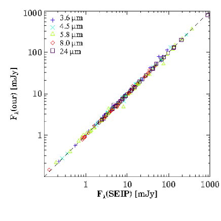
Figure 2: SEIP Source List fluxes of a sample of candidate YSOs plotted against those measured during the present work.

Due to the strict quality requirements of the SEIP Source List several sources might have been missed in one or more bands. Furthermore, the 70-µm data are not included in the SEIP data base. Therefore we checked the positions of the selected sources and performed photometry by the procedures described in Kun et al. (2014) to refill the missing flux data. Then we checked the 70-µm images at each source position and measured 70-µm fluxes. Figure 2 compares our photometry with the SEIP Source List data.

2.2 High Angular Resolution Near-infrared Imaging

High angular resolution near-infrared images of two small regions of L1340 were obtained on 2002 October 24 in the JHK bands, using the near-infrared camera Omega-Cass, mounted on the 3.5-m telescope at the Calar Alto Observatory, Spain. Our targets were IRAS 02224+7227, the possible driving source of HH 487, and the compact, partly embedded cluster RNO 7, centred on IRAS 02236+7224. The results for IRAS 02224+7227 have been shown in Kun et al. (2014). Here we present the results for RNO 7.

Omega Cass’s detector was a Rockwell $1024\times 1024$ pixel HAWAII array (HgCdTe detector + Si MOSFET non-destructive readout). The plate scale was 0.1″/pixel. RNO 7 was observed at four dithering positions around the nominal position of IRAS 02234+7224, and the observations consisted of two dither cycles, and each cycle with 120 s ($4\times 30$ s in J and H, $12\times 10$ s in K) spent at each position. Thus, the total on-source integration time of a cycle was 480 s in each filter. Double Correlated Read (Reset-Read-Read) was applied.

The data were reduced in IRAF. Following the flat-field correction and bad pixel removal the sky frame for each cycle was obtained by taking the minimum of the images at different dithering positions. This sky frame was subtracted from each individual image of a given cycle. Then the frames from a single cycle were combined into a mosaic image, and aperture photometry was performed on the reduced images. The instrumental magnitudes were transformed into the JHK_s system by using the 2MASS magnitudes of 17 stars within the field of view. Then, in order to search for possible close visual companions, the point spread function of the images were determined and the scaled psf of the stars were subtracted from the images.

2.3 Supplementary Data

To classify the evolutionary status of the color-selected candidate YSOs and obtain as complete picture of the star-forming region and its YSO population as possible, we supplemented the Spitzer data with photometric data available in public data bases. The data bases included in our study are as follows.

2MASS and AllWISE data

The SEIP Source List contains WISE and 2MASS associations of the catalogued objects. WISE 22-µm fluxes exist for 24 Spitzer-selected candidate YSOs outside of the area of the 24-µm MIPS observations. We included these association into the analysis, taking into account that, due to the different angular resolutions, a few 2MASS/WISE sources are associated with more than one IRAC source. Furthermore we searched the AllWISE Source Catalog (Wright et al., 2010) for young stellar objects, using the color and flux criteria established by Koenig et al. (2012, 2014). We identified eight new candidate YSOs, seven of which are located outside of the field of view of the Spitzer observations.

Akari FIS/IRC data

Akari far-infrared all-sky survey images (Doi et al., 2015), tracing out the surface and temperature structure of the cold dust in the cloud region, are accessible at http://www.ir.isas.jaxa.jp/AKARI/Archive/Images/FISMAP/. We identified counterparts of 9 candidate YSOs the Akari/FIS Bright Source Catalogue (Yamamura et al., 2010), containing point sources detected at 65, 90, 140, and 160 µm.

Submillimeter data

Part of the molecular clump L1340 B was observed at 450 and 850 µm with the Submillimetre Common User Bolometer Array (SCUBA) on the James Clerk Maxwell Telescope. The outlines of the mapped area are shown in fig. 6 of Paper III. The 850 µm image and positions, sizes and fluxes/upper limits of nine submillimeter sources can be found in the SCUBA Legacy Catalogues (Di Francesco et al., 2008), at http://www3.cadc-ccda.hia-iha.nrc-cnrc.gc.ca/community/scubalegacy/. Four of them coincide in position with Spitzer sources.

Herschel data for L1340 C

The Planck Galactic cold clump PGCC G130.38+11.26, associated with L1340 C, was included in the detailed Herschel study of cold clumps by Juvela et al. (2012). Far-infrared images, observed by the PACS instrument at 100 and 160 µm, as well as 250, 350, and 500 µm images observed by the SPIRE instrument are available in the Herschel Science Archive (http://www.cosmos.esa.int/web/herschel/science-archive). We found far-infrared counterparts of 20 color-selected Spitzer sources in the PACS 100 and 160 µm images. We measured the fluxes of the sources on the level2.5 JScanam images, downloaded from the Herschel Science Archive (Galactic Cold Cores: A Herschel survey of the source populations revealed by Planck, PI: M. Juvela). The photometry was performed using the L3_multiplePointSourceAperturePhotometry.py, supplied in HIPE 14.0 RC4 (Herschel Interactive Processing Environment, Ott, 2010). We used 6″  and 10″ apertures at 100 µm  and 160 µm, respectively, with an annulus between 35″ and 45″ for determining the background. The aperture correction were calculated using the values given in Balog et al. (2014). The initial positions of the sources were taken from the SEIP Source List and were refined using a two dimensional Gaussian during the photometry.

SDSS data

SDSS ugriz magnitudes are available for each star brighter than some 25 mag in each band within the whole area of L1340 (see Paper III). We searched for counterparts of our candidate YSOs the SDSS Data Release 9 (Ahn et al., 2012) within 1″  to the SEIP Source List position. We transformed the SDSS magnitudes of the optical counterparts into the Johnson–Cousins UBVR_CI_C system, using the equations given in Ivezić et al. (2007) (for BVR_CI_C) and Jordi et al. (2006) (for U). We found optical counterparts for 149 of the 155 Class II Spitzer sources, and for 8 of the 26 Flat SED sources (see Sect. 4.1).

3 INFRARED APPEARANCE OF L1340: THE SWAN NEBULA

The extended infrared emission reveals the surface distribution of various components of the cloud. Cold ($T_{\mathrm{kin}}\sim$10–20 K), big ($r\gtrsim 0.1$ µm) dust grains radiate in the far-infrared, whereas extended mid-infrared emission traces out very small grains and excited PAH molecules. Heating and shocks from embedded YSOs also appear in the infrared images of a molecular cloud.

Figure 3 shows a three-color view of L1340, composed of the WISE 4.6 µm (blue), 12 µm (green), and 22 µm (red) images. Striking features of this image are the bright, extended 12-µm radiation, indicative of PAH emission excited by B and A type stars, and small groups of 22-µm sources, associated with the three cloud clumps. The shape of the brightest part of the diffuse 12-µm  emission, located slightly northwest of the image centre, and associated with the clump L1340 B, suggests the Swan nebula label.

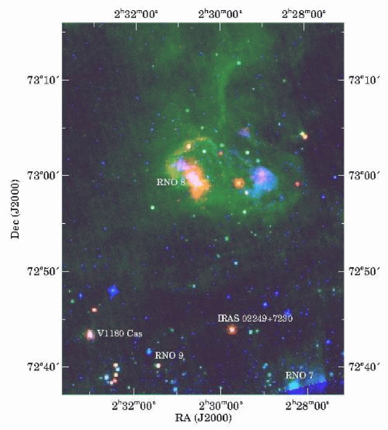
Figure 4: Three-color image of a $29\arcmin\times 39\arcmin$ size part of L1340, composed of Spitzer IRAC 5.8 µm (blue), MIPS 24 µm (green), and MIPS 70 µm images. Part of L1340 A is outside the field of view of the MIPS images.

Figure 4 is a composite of the 5.8 µm  IRAC (blue), 24 µm  MIPS (green), and 70 µm  MIPS (red) images. The image reveals an extended 70-µm structure associated with RNO 8, diffuse 24-µm emission which delineates the Swan nebula, a bluish (5.8 µm) glowing around the B-type stars, and a variety of far-infrared point sources.

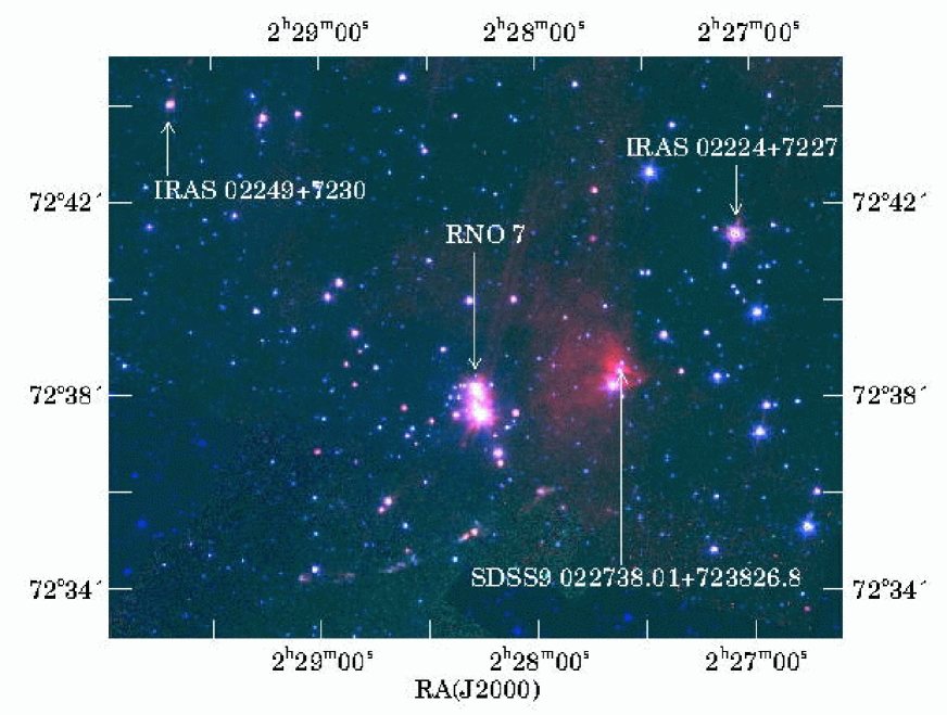
Figure 5: Three-color image of the cloud clump L1340 A, composed of Spitzer IRAC 3.6 µm (blue), 5.8 µm (green), and 8.0 µm (red) images. The size of the image is about $15.6\arcmin\times 12\arcmin$. The arrows point to the positions of the FUor-like YSO IRAS 02224+7227, the A0-type star SDSS9 J022738.01+723826.8, associated with extended 8-µm emission, the protostar IRAS 02249+7230, and the RNO 7 cluster.

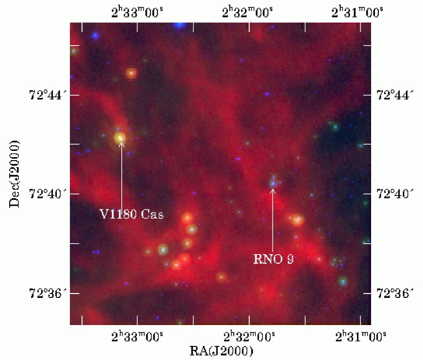
Figure 7: Three-color image of the clump L1340 C, composed of Spitzer IRAC 3.6 µm (blue), MIPS 24 µm (green), and Herschel SPIRE 250 µm (red) images.

To reveal further details of the diffuse infrared emission of L1340, we present three-color images of the clumps L1340 A, L1340 B, and L1340 C in Figs. 5, 6, and 7, respectively. Figure 5 is composed of IRAC 3.6 µm (blue), 4.5 µm (green), and 8.0 µm  (red) Super Mosaic images of L1340 A (much of this clump is outside of the MIPS images). Conspicuous features of the image are a diffuse 8-µm emission around the A0 type star SDSS9 022738.01+723826.8 (Paper III), the nebulous RNO 7 cluster, and HH 488, stretching from NW towards SE near the southern boundary of the image. Figure 6 is composed of the 3.6 µm  (blue), 8.0 µm  (green), and 24 µm (red) images of the most massive clump L1340 B. The wispy structure of the Swan nebula, suggesting a swirling gas cloud, becomes apparent in this image. A bow-shock like feature can be seen around the star SDSS9 J023049.80+730110.2, demonstrating supersonic motion of the gas with respect to the A2-type, young intermediate-mass star (Paper III). The extended infrared emission from the smallest clump, L1340 C, shows up in the Herschel images, tracers of very cold dust. Figure 7, composed of the 3.6 µm IRAC (blue), 24 µm MIPS (green), and 250 µm SPIRE (red) images of the central $12\arcmin\times 12\arcmin$ area of L1340 C reveals a complex network of filamentary dust formations.

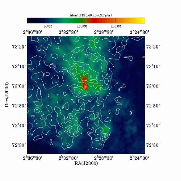
Figure 8: Akari Wide-L map of L1340 (colors) with the visual extinction (white solid contours, Kun et al., 2016) overplotted. Both the lowest contour and increment for $A_{\mathrm{V}}$ are 1.0 mag. The center coordinates and size of the image are identical with those in Fig. 3.

The Akari Wide-L band image, centered on 140 µm, is displayed in Fig. 8, with the contours of the visual extinction (Paper III) overplotted. The Figure indicates that both the 140-µm emission and the visual extinction trace the same component of the cloud. The lowest contour at $A_{\mathrm{V}}=1.0$ mag largely follows the 40–50 MJy sr^-1 level of the far-infrared emission. At a few positions, heated by embedded YSOs, the strong 140-µm emission is not associated with high extinction.

4 YOUNG STELLAR OBJECTS IN L1340

4.1 Spitzer Sources

4.1.1 SED-based Classification

We classified the candidate YSOs, selected by the color criteria described in Sect. 2.1, based on the slope of their spectral energy distributions (SEDs), $\alpha=d\log(\lambda F(\lambda))/d\log\lambda$. We derived $\alpha$ both for the $K_{\mathrm{s}}$ –24 µm and the 3.6 µm–8.0 µm intervals (for 3.6 µm–5.8 µm when 8 µm observations were missing). We used the WISE 22 µm data when 24 µm MIPS data were missing. According to the canonical classification scheme (Lada, 1991; Greene et al., 1994), protostellar objects embedded in an envelope have $\alpha(2-24)>0.3$, whereas $\alpha(2-24)<-0.3$ for pre-main sequence stars surrounded by accretion disks. Flat SED sources with $-0.3\leq\alpha(2.0-24.0)\leq 0.3$ represent the transition between the protostellar and pre-main sequence evolutionary phases. We classified 155 Class II, 45 Class I, and 25 Flat SED sources. We detected a further Class I/Class 0 source in the 70-µm MIPS image at $02^{\mathrm{h}}29^{\mathrm{m}}56\fs 90$, $+73\arcdeg 02\arcmin 17\farcs 0$. This source is undetectable at shorter wavelengths, and coincides in position with an Akari FIS source and with a submillimeter source.

4.1.2 Estimating Foreground Extinction

Since the classification based on observed spectral slopes is biased by the extinction of the sources, we estimated the foreground extinctions of the candidate YSOs, and then reclassified them according to the extinction-corrected SED slopes. Foreground extinctions of Class I and Flat SED sources were estimated using the extinction map, derived from SDSS star counts in Paper III. We adopted the pixel value of the extinction map at the position of the source as the foreground extinction of an embedded source. On the one hand, the extinction obtained in this manner is an upper limit, since the sources may be situated at any depth within the dusty medium. On the other hand, small-scale, high-extinction cores, missed by the extinction mapping, may be present around embedded sources. For the Class II sources we invoked SDSS and 2MASS  counterparts. We compared the optical and near-infrared side (from the B to the J band) of the SED with a grid of reddened photospheres, following the method described in Paper III, and thus estimated the spectral type and extinction of the central star. Based on the slopes of the extinction-corrected SEDs, two sources, classified originally as Class I, moved into the Flat class, and one Flat SED source moved into the Class II sample. Tables 1, 2, and 3 list the SSTSL2 identifiers and Spitzer fluxes of the Class 0/I, Flat SED, and Class II sources of L1340, respectively.

The SEDs of Class II sources can be divided into further subclasses by comparing the dereddened SED slopes with the median band of the Taurus pre-main sequence sample (D’Alessio et al., 1999; Furlan et al., 2006). The SED subclasses are indicative of the dust distribution in the circumstellar disks (Evans et al., 2009) of the classical T Tauri stars, and may shed light on the processes governing disk evolution. We classified the infrared excesses of our candidate pre-main sequence stars into three groups: (1) the SED of primordial disks (II P subclass) does not drop below the Taurus median band; (2) the SED of the weak or anemic disks (II A subclass) is below the Taurus band over the whole observed wavelength region, and (3) pre-transitional and transitional disks (II T) have SEDs below the Taurus median band at intermediate wavelengths, and start rising above 20 µm. For this latter group the spectral index $\alpha(8-24)>0$.

4.1.3 Submillimeter, Far-infrared, and Optical Counterparts

Six Spitzer  sources are associated with submillimeter sources listed in the JCMT SCUBA Fundamental Catalogue (Di Francesco et al., 2008). Far-infrared counterparts of 17 candidate Class 0/I, and three Flat SED YSOs were identified in the Herschel PACS images. Table 4 lists the SSTSL2 associations, 100 µm, and 160 µm fluxes of these Herschel point sources.

Nine of the Spitzer-selected candidate YSOs coincide in position with far-infrared sources detected by the Akari/FIS instrument (Kawada et al., 2007). Four of them are included in the Akari/FIS young stellar object catalog (Tóth et al., 2014). A fifth catalog entry, Akari 0232291+723855, has an associated mid-infrared point source, AllWISE 023227.63+723841.4, within the half-maximum radius of the point-spread function of the FIS (Arimatsu et al., 2014). Its fluxes, however, probably originate from more than one sources. Similarly, the far-infrared fluxes of Akari FIS 0230333+725951, a bright candidate YSO detected in each FIS band and associated with IRAS 02259+7246, are composed of several sources. An extended emission can be seen around this position in the Spitzer 70-µm image. We found SDSS counterparts of all but seven Class II infrared sources. A few Flat and Class I sources also have SDSS counterparts. Most of these counterparts are classified as galaxies. The non-stellar appearance, however, may indicate their scattered light origin.

SDSS, 2MASS, AllWISE, Akari, and other identifiers of Class I and Flat sources are listed in Tables 5 and 6, respectively. For the Class II sample, excluded the 65 members common with the H$\alpha$ emission stars studied in Paper III, we give the UBVR_CI_CJHK_s magnitudes in Table A1 of the Appendix.

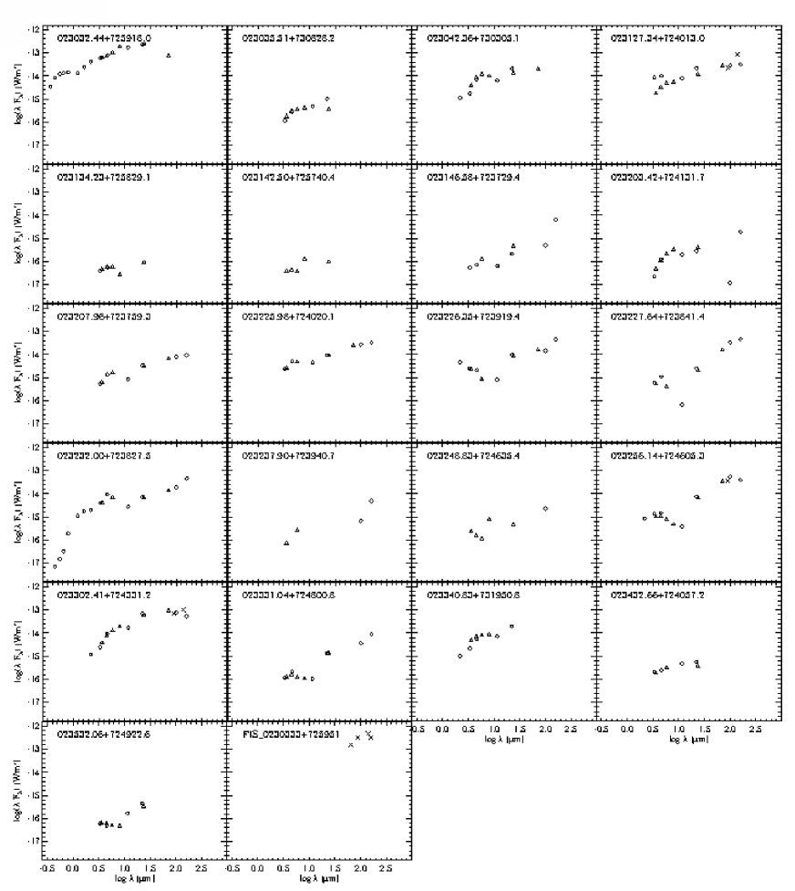
Figure 9: SEDs of the Class I YSOs (continued).

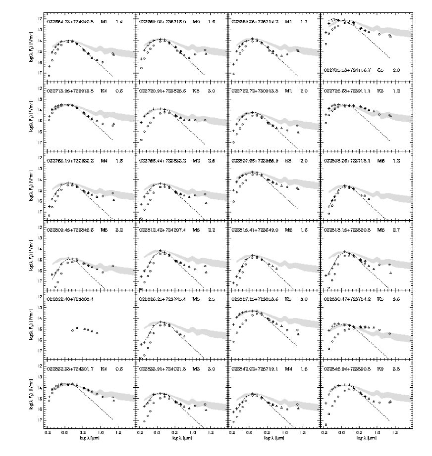
Figure 11: SEDs of the Class II candidate YSOs identified in the SEIP Source List data, and not identified as H$\alpha$ emission stars. The SEDs of H$\alpha$ emission stars can be seen in fig. 9 of Paper III. Open circles show the SDSS, 2MASS, and WISE data, and triangles are for Spitzer data. Plusses indicate the dereddened SED, and the dashed line shows the photospheric SED of the spectral type, obtained by fitting a model to the data. The gray shaded area indicates the median SED of the T Tauri stars of the Taurus star-forming region (D’Alessio et al., 1999). SSTSL2 identifiers, spectral types, and $A_{\mathrm{V}}$ extinctions, derived from photometric data are indicated at the top of each panel.

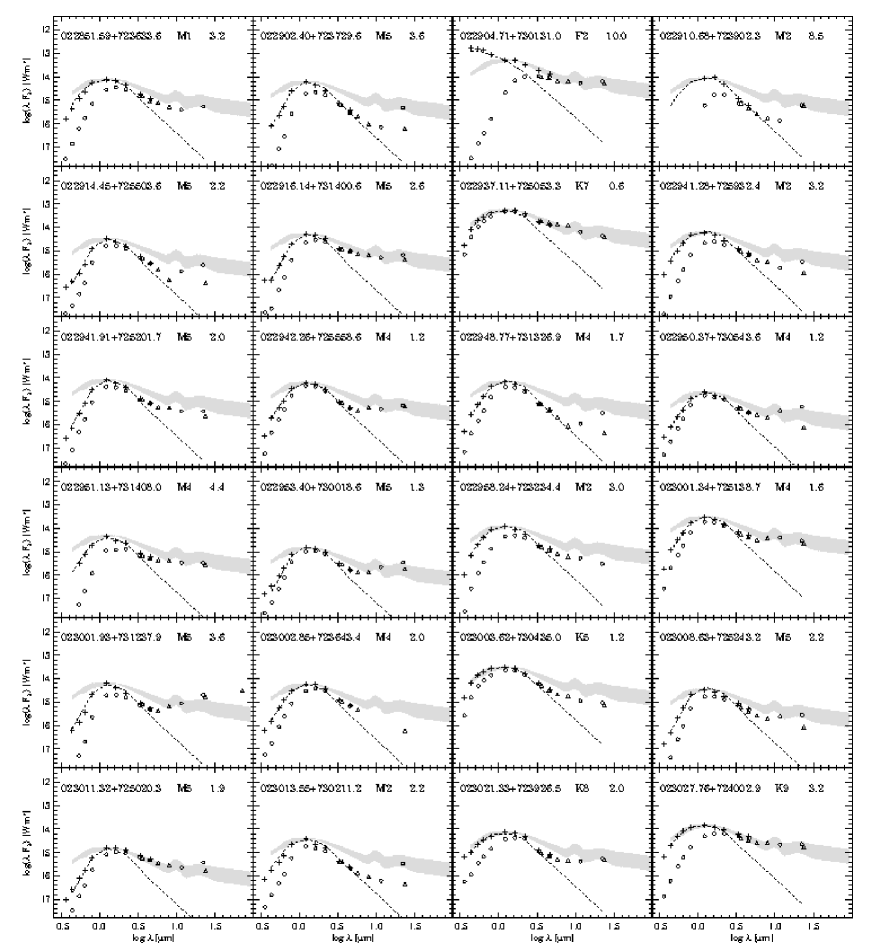
Figure 11: SEDs of the Class II candidate YSOs (continued).

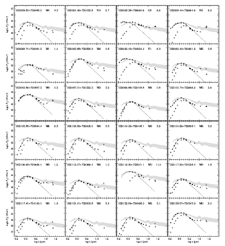
Figure 11: SEDs of the Class II candidate YSOs (continued).

The SEDs of the candidate YSOs, constructed from all available data, are displayed in Fig. 9, 10, and 11 for the Class I, Flat, and Class II sources, respectively. Since the SEDs of the H$\alpha$ emission stars, together with those of the best-fitting photospheres, have been presented in fig. 9 of Paper III, Fig. 11 presents the results for the Class II subsample not detected as H$\alpha$ emission stars during our slitless spectroscopic H$\alpha$ survey. The dereddened SEDs, as well as the best fitting photosphere (Pecaut & Mamajek, 2013) are also plotted, and the derived spectral type and extinction are indicated in each plot.

4.1.4 Bolometric temperatures and luminosities

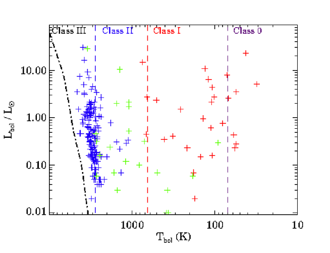
Figure 12: Extinction-corrected bolometric luminosities plotted against extinction-corrected bolometric temperatures. Red crosses indicate Claas 0/I sources, green symbols are for Flat, and blue for Class II SED slopes. Vertical dashed lines indicate the boundaries between the Classes, and the dash-dotted line indicates the position of the zero-age main sequence (Siess et al., 2000).

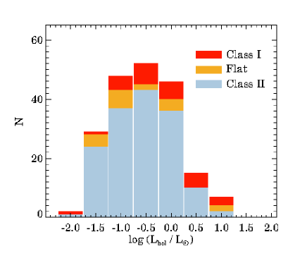
Figure 13: Histogram of bolometric luminosities of Class 0/I/Flat protostars and Class II pre-main sequence stars.

Bolometric temperatures and luminosities, as defined in Myers & Ladd (1993), were derived from the dereddened SEDs for the Class I and Flat SED objects, detected at least in one band beyond 24 µm, and for the Class II sources, detected over the 0.36–24 µm region. Akari FIS, Herschel PACS, and JCMTSF submillimeter data were included into the integration when available. Contribution of the spectral regions beyond the longest wavelength was estimated using the method described by Chavarría-K. (1981). The $L_{\mathrm{bol}}$ vs. $T_{\mathrm{bol}}$ diagram of the candidate YSOs is plotted in Fig. 12. The YSO Classes, defined by the spectral slopes, correspond to the $T_{\mathrm{bol}}$ intervals indicated in Fig. 12 (Chen et al., 1995). It can be seen that both $\alpha(2-24)$ and $T_{\mathrm{bol}}$ are consistent with the Class 0/I identification. Flat SED sources overlap in $T_{\mathrm{bol}}$ with both Class I and Class II, whereas a significant part of the Class II sample has $T_{\mathrm{bol}}$ above the theoretical boundary of 2800 K. It is in accordance with the recent finding of Dunham et al. (2015), that the extinction-corrected $T_{\mathrm{bol}}$ of a Class II source depends on the $T_{\mathrm{eff}}$ of the central star, rather than on the disk properties. Figure 13 shows the histogram of bolometric luminosities of the candidate YSOs. The mean $L_{\mathrm{bol}}$ of the 28 Class I sources, detected at $\lambda>24$µm, is $\langle L_{\mathrm{bol,ClassI}}\rangle=3.4~{}L_{\sun}$, and the same for the Class II sample is $\langle L_{\mathrm{bol,ClassII}}\rangle=1.2~{}L_{\sun}$.

Tables 7 and 8 present the derived extinctions, extinction-corrected SED slopes, bolometric temperatures and luminosities of Class 0/I and Flat SED sources, respectively. Table 9, in addition to the above quantities, lists the derived spectral types and luminosities for central stars of the Class II sources, as well as the SED subclasses.

4.2 New Candidate Members of RNO 7 in the Omega-Cass Data

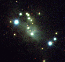
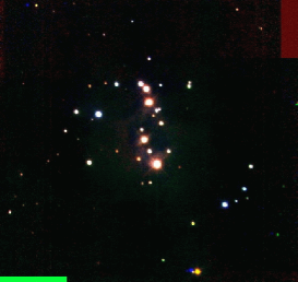
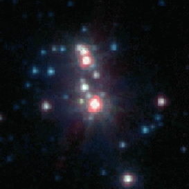
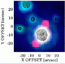
Figure 14: Optical, near-infrared, and mid-infrared three-color composite images of RNO 7. The upper left panel is composed of the SDSS g (blue) r (green), and i (red) images, the upper right panel resulted from our high angular resolution J (blue), H (green), and K (red) observations, and the lower left panel presents a composite of the Spitzer IRAC 3.6 µm (blue), 4.5 µm (green), and 8.0 µm (red) images. The lower right panel magnifies a $30\arcsec\times 30\arcsec$ area of the previous image around the brightest member of the cluster. The IRAC composite image is scaled to show the two faint, 8-µm companions, and Omega-Cass $K$-band contours, revealing a close near-infrared companion, are overplotted.

The three-color composite of the J (blue), H (green), and the K (red) Omega-Cass images is shown in the second panel of Fig. 14. For comparison, we show in the first panel an optical three-color view of the same region, composed of the SDSS g (blue), r (green), and i (red) images, whereas the third panel shows the Spitzer 3.6 µm (blue), 4.5 µm (green), and 8 µm (red) composite image. The high angular resolution Omega-Cass images reveal a few new objects, detectable neither in the optical nor in the IRAC images. Furthermore, they show that the brightest member of RNO 7, SSTSL2 J022816.62+723732.6, associated with IRAS 02236+7224, has a faint companion at an angular distance of 1.12″ (Fig. 14, fourth panel), corresponding to some 760 AU at a distance of 825 pc.

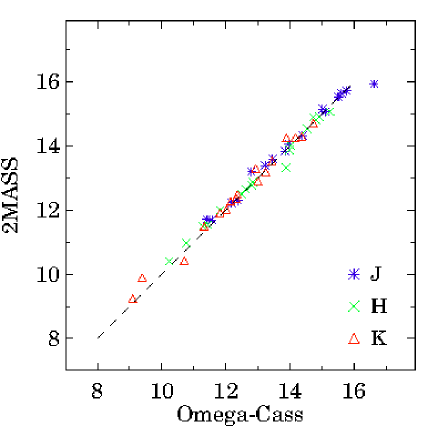
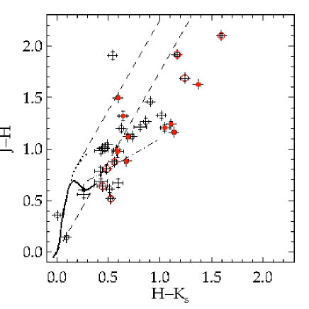
Figure 15: Left: 2MASS magnitudes of 17 stars within the field of view of the Omega-Cass, plotted against those measured in the Omega-Cass images. Right: $J-H$ vs. $H-K_{\mathrm{s}}$ two-color diagram of the stars in the region of RNO 7, detected in each band in the Omega-Cass images, and listed in Table 10. Solid line indicates the colors of the main sequence stars, and dotted line shows those of the giants (Bessell & Brett, 1988). Dashed lines border the band of the reddened main sequence and giant stars, and the dash-dotted line is the locus of T Tauri stars (Meyer et al., 1997). Red dots indicate the known H$\alpha$ emission stars, and open circles show the stars selected as Class II infrared sources in the Spitzer data.

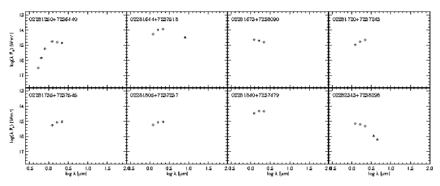
Figure 16: SEDs of the candidate young stars identified in the Omega-Cass JHK data.

The magnitudes measured in the Omega-Cass images, and transformed into the 2MASS system, are compared with the 2MASS magnitudes of the same stars in the left panel of Fig. 15. The right panel of Fig. 15 shows the J$-$H vs.H$-$K_s two-color diagram of the stars measured in each band. Twenty stars are located to the right of the band of the reddened normal main sequence and giant stars, indicating K_s-band excess. Table 10 lists the derived magnitudes of these stars. All but two of them have 2MASS counterparts, but none of them has good (A or B) photometric quality in each band. Six of the 14 H$\alpha$ emission stars, discovered by Magakian et al. (2003), and seven Spitzer-identified candidate YSOs are found in this sample. Eight stars, marked with asterisks in Table 10, are new candidate members of RNO 7. The SEDs of these eight stars, constructed from all available data, are presented in Fig. 16.

4.3 AllWISE sources

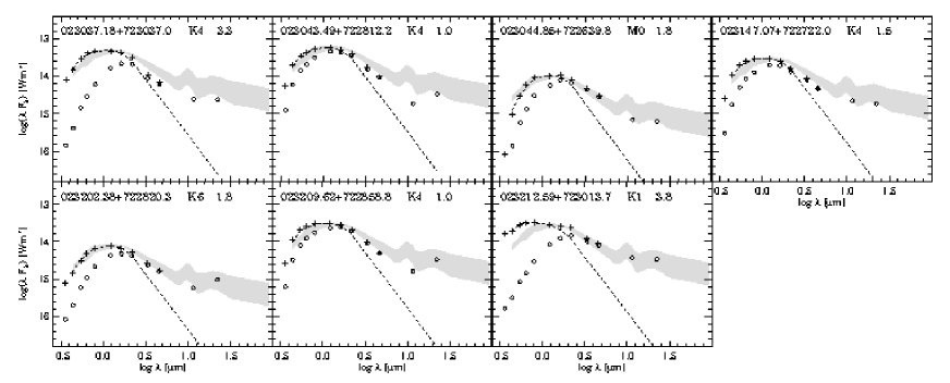
Figure 17: SEDs of the candidate young stars identified in the AllWISE data, located outside of the field of view of the Spitzer observations.

The 1 square degree area centered on RA(J2000) = 37$\fdg$625, Dec(J2000) = +72$\fdg$933 contained 954 sources, having signal to noise ratio greater than 5.0 in each band and not affected by upper-case contamination flag. We identified seven new Class II source candidates in the WISE  database outside the area covered by the Spitzer images, but within the lowest significant ¹³CO contours of the molecular cloud. Each of them is located near the southern boundary of the cloud. Furthermore, two WISE  sources without coinciding SSTSL2 entries, J022759.92+723556.4 and J023227.63+723841.4 were found within the field of view of the Spitzer observations. We measured their fluxes in the available bands, and added the sources to Tables 2 and 1, respectively. The selected AllWISE sources are listed in Table 11. The SEDs of the seven WISE sources, identified as candidate YSOs outside the field of view of the Spitzer observations, are displayed in Fig. 17. Each of them is a Class II source. Their $A_{\mathrm{V}}$ extinctions, spectral types, and luminosities derived from the photometric data, are listed in Table 12.

4.4 Embedded Protostars and Herbig–Haro objects in L1340

4.4.1 Candidate Class 0 Sources

The extinction-corrected SED slopes revealed the presence of 45 Class 0/I and 27 Flat SED candidate YSOs. Eight sources have $T_{\mathrm{bol}}\lesssim 70$ K, suggesting Class 0 evolutionary stage (Myers & Ladd, 1993). These are as follows.

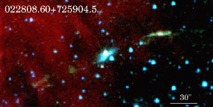
Figure 18: RGB image composed from IRAC 8 µm (red), 4.5 µm (green), and 3.6 µm (blue) images of the candidate Class 0 protostar SSTSL2 J022808.60+725904.5. The 4.5 µm knots at both side of the nebulous source indicate HH objects driven by the Class 0 protostar, and corresponding to the protostellar outflow reported in Walawender et al. 2016.

• SSTSL2 J022808.60+725904.5 coincides with an Akari FIS and a JCMTSF submillimeter source (see Table 5). Its SED, assembled from all available data (Fig. 9), shows deep silicate absorption around 10 µm, suggesting a Class 0 protostar seen at high inclination (Enoch et al., 2009). This object is associated with a parsec-scale outflow identified in H₂ 2.12-µm observations (J. Walawender et al. 2016, in prep.). The three-color image of its environment, composed of IRAC 8 µm (red), 4.5 µm (green), and 3.6 µm (blue) images and displayed in Fig. 18, shows 4.5-µm emission, originating from shocked H₂.

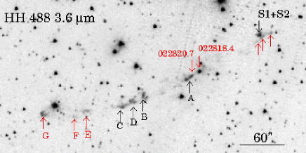
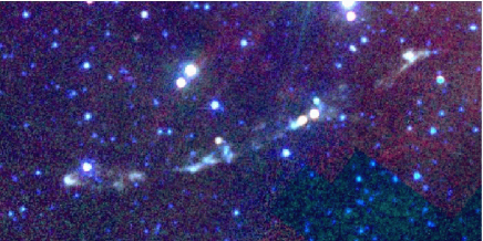
Figure 19: Top: HH 488 in the 3.6 µm  IRAC band. The HH knots A, B, C, D, and the binary star S1+S2, driving source candidate identified by Kumar et al. (2003) are indicated by the black characters, and red characters mark the new protostars SSTSL2 022818.51+723506.2 and SSTSL2 022820.81+723500.5, and HH knots E, F, G, revealed by the Spitzer images. Bottom: Three-color image of the same region, composed from IRAC 8 µm (red), 5.8 µm (green), and 3.6 µm (blue) images.

• SSTSL2 J022820.81+723500.5 lies outside the MIPS 70-µm image. Its steeply rising SED is revealed by the Akari FIS data. With $L_{\mathrm{bol}}\approx 23$ $L_{\sun}$ it is the most luminous protostar of L1340. This source, together with another nearby Class I source 022818.51+723506.2, is located along the chain of Herbig–Haro objects HH 488 whose several knots were detected in optical H$\alpha$ and S II images by Kumar et al. (2003) and Magakian et al. (2003). Kumar et al. (2003) suggested that the driving source was the brighter component of a binary star located at $2^{\mathrm{h}}28^{\mathrm{m}}00^{\mathrm{s}},72\arcdeg 35\arcmin 58\arcsec$ (HH 488 S, Source 2 in Table 2). The optical counterpart of HH 488 S is classified as a galaxy in the SDSS DR9, and as an HH object by Magakian et al. (2003). Our photometry suggests a Flat SED, although it results from the composite fluxes of the central objects. The positions of the two protostars with respect to the HH knots suggest that either of them is the probable driving source. The IRAC images reveal new knots of HH 488. In the upper panel of Fig. 19 we marked the known and new knots of HH 488 and the candidate driving sources. The lower panel shows a three-color composite image of HH 488, whose angular extension of 5.6′ corresponds to a total length of some 1.3 pc at a distance of 825 pc.

• SSTSL J022931.98+725912.4 is associated with IRAS and Akari far infrared, and JCMTSF submm source (Table 7). It is associated with a small fan-shaped reflection nebulosity, bright at 3.6 µm on the eastern side, and a jet-like feature, bright at 4.5 µm on the western side (Fig. 20).

• The fourth candidate Class 0 protostar is the 70-micron source No. 22 in Table 1. It is associated with the brightest submillimeter source of the region.

• SSTSL 023256.14+724605.3 is an embedded eruptive young star in L1340 C, discussed in (Kun et al., 2014). Its $T_{\mathrm{bol}}$ and $L_{\mathrm{bol}}$ were determined including the Herschel 100 µm and 160 µm fluxes.

• SSTSL 023146.58+723729.4, 023237.90+723940.7, and 023330.92+724800.3 are low-luminosity sources, not detected in the 70 µm MIPS image. Their low bolometric temperatures were revealed by including the Herschel 100 µm and 160 µm data into the SEDs. Their nature is uncertain: they may be either very low luminosity protostars or faint distant galaxies.

4.4.2 Class I protostars associated with IRAS sources

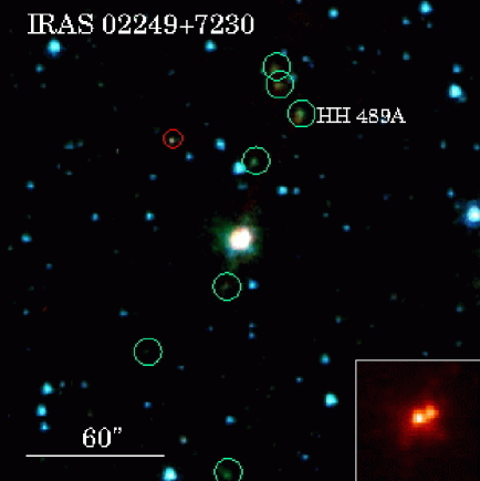
Figure 21: Three-color image, composed from the IRAC 3.6 µm (blue), 4.5 µm (green), and 8 µm (red) images of the environment of the binary protostar IRAS 02249+7230, the driving source of HH 489. HH 489 A, and further HH objects revealed by the 4.5-µm image are marked by the green circles. The faint red object within the red square is another Class I object SSTSL2 J022950.37+724441.4. The inset in the lower right corner shows the 30″ environment of the central object, magnified and scaled for better visibility.

Six IRAS sources, listed in table 6 of Paper I, are associated with Class I Spitzer sources (see Table 5). IRAS 02249+7230 in L1340 A is the driving source of HH 489 (Magakian et al., 2003). The Spitzer data show it to be a wide binary, consisting of two Class I sources, SSTSL2 J022943.01+724359.6 and SSTSL2 J022943.64+724358.6, separated by 2.8″. Their SEDs are shown in Fig. 9, and the environment is displayed in the three-color image in Fig. 21. HH 489 A, identified in optical H$\alpha$ and S II images by Magakian et al. (2003) as well as a chain of faint HH knots to the south can clearly be seen. Their projected distribution suggests that both components of the binary and another nearby Class I source, SSTSL2 J022950.37+724441.4 may contribute to their excitation.

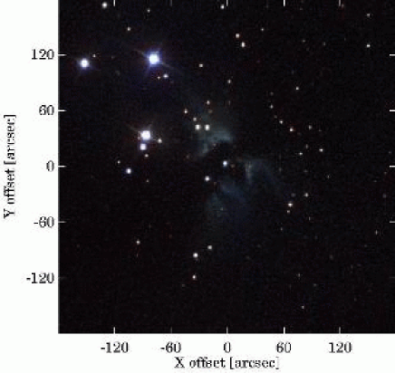
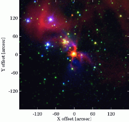
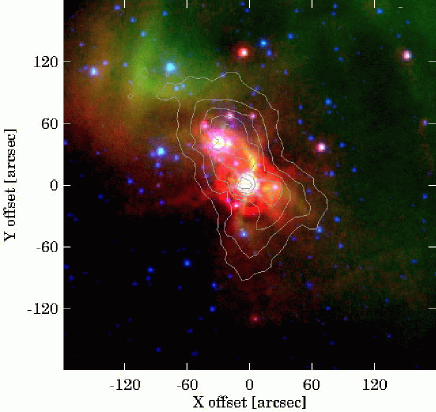
Figure 22: First panel: Optical three-color image of RNO 8, composed from the SDSS g (blue), r (green), and i (red) images. Second panel: three-color image of the same region composed of SDSS g (blue), IRAC 3.6 µm (green), and IRAC 8 µm (red) images. Third panel: Three-color image composed of the IRAC 4.5 µm (blue), 8.0 µm (green), and MIPS 24 µm (red) images. Light grey contours show distribution of the 70 µm  emission.

Figure 12 shows that $T_{\mathrm{bol}}$ of the second brightest Class I object of L1340 falls into the Class II regime near the Class I/Class II boundary. This ambiguous classification belongs to SSTSL2 J023032.44+725918.0, associated with IRAS 02259+7246 and RNO 8. A faint optical star is visible at its position. Our low-resolution spectrum (Paper III) reveals its late G spectral type with the Balmer lines in emission, and the optical color indices point to an unreddened star. The bolometric luminosity, determined from the $I_{\mathrm{C}}$ or J magnitudes, places this star near the ZAMS. All these data suggest the high inclination of the disk of this star. The optical and infrared images confirm this statement. Three-color images, shown in Fig. 22, reveal the connections between various components of the circumstellar environment of RNO 8. The gap between the star and the nebulosity in the optical three-color image (first panel of Fig. 22) suggests a huge shadow of the circumstellar disk on the dusty envelope, stretching far beyond the disk. The image composed of the optical g (blue), IRAC 3.6 µm (green), and IRAC 8 µm  (red), and shown in the second panel of Fig. 22, reveals streaks of 8-µm  emission overlapping with the reflected starlight. The image in the third panel is composed of the 4.5 µm (blue), 8 µm (green), and 24 µm (red) images. The overplotted contours of the 70 µm emission reveal a cloud core associated with RNO 8.

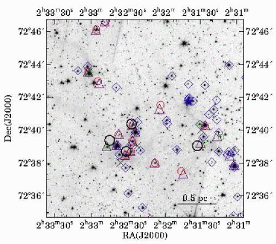
Figure 29: Surface distribution of the candidate YSOs and dense NH₃ cores in a $12\arcmin\times 12\arcmin$ area of L1340 C. Symbols are same as in Fig. 27, and triangles indicate far-infrared sources detected in the Herschel PACS images.

In L1340 C a J-shaped chain, consisting of five Class I and four Class II YSOs, can be seen close to the extinction peak (see Fig. 29). IRAS 02276+7225 and Akari FIS 0232291+723855 are situated in the same area, but neither of them can be unambiguously associated with mid-infrared sources. Similarly, IRAS 02267+7226 and Akari FIS 0231270+724015 coincide with the Class I source SSTSL2 J023127.34+724012.9 within the position uncertainties, but other nearby sources may contribute to their catalogued fluxes.

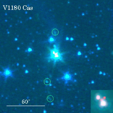
Figure 23: Same as Fig. 20, for the environment of V1180 Cas. In addition to the jet, emanating northward from the Class I component (Antoniucci et al., 2014), several fainter HH knots can be detected. A third component of the system emerges in the 8-µm image. The inset shows a $18\arcsec\times 18\arcsec$ area of the central objects.

SSTSL2 J023302.41+724331.2, coinciding with IRAS 02283+7230, is the Class I companion of the eruptive star V1180 Cas. This protostar drives a jet, detected by Antoniucci et al. (2014) in [S II] and H$\alpha$ narrow-band images. The IRAC 4.5 µm image also clearly show the jet (Fig. 23), as well as several faint HH objects. The 8-µm image reveals a probable third component of the system, located at $4.8\arcsec$ towards the north-northwest from V1180 Cas.

IRAS 02240+7259, detected at 100 µm only by IRAS and thus not listed in Paper I, coincides with a faint candidate protostar SSTSL2 J022855.69+731333.1, not detected at 70 µm. Taking into account the IRAS 100-µm flux the SED suggests a Class 0/I source with $T_{\mathrm{bol}}\approx 75$ K. The nature of this source, however, is uncertain: it may be a distant galaxy.

4.5 Classical T Tauri stars

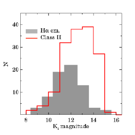
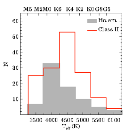
Figure 24: Histogram of the K_s magnitudes (left), visual extinctions (middle), and effective temperatures/spectral types (right), derived from photometric data of the candidate pre-main sequence stars of L1340.

The Spitzer, WISE, and Omega-Cass data resulted in 170 Class II young stars in the region of L1340. These stars represent the classical T Tauri star (CTTS) population of L1340. Sixty-five of the 77 H$\alpha$ emission stars, presented in Paper III, are members of this sample. These stars are marked with asterisks in Tables 3 and 9. Histograms of their K_s magnitudes, derived $A_{\mathrm{V}}$ and $T_{\mathrm{eff}}$ values are shown in Fig. 24, together with those of the H$\alpha$  emission subset (Paper III). It can be seen that H$\alpha$ emission was detected in brighter and hotter Class II stars. Only five of the Class II stars brighter than $K_{\mathrm{s}}=11.5$ were not detected during the H$\alpha$ survey, and only one H$\alpha$ emission star has spectral type later than M2. The derived extinctions of the Class II sources peak between $2~{}mag<$ A${}_{\mathrm{V}}<3~{}mag$.

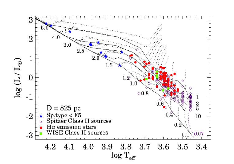
Figure 25: Hertzsprung–Russell diagram of the candidate young population of L1340. Blue star symbols indicate the stars earlier than F5 (Paper III), red filled circles show Class II sources with H$\alpha$ emission detected (Paper III). Open diamonds indicate Class II sources not detected during our H$\alpha$ survey. Black dotted lines indicate evolutionary tracks, and thin solid lines mark the 1, 3, 5, 10 million year isochrones from Siess et al. (2000). The track for 0.07 M_☉ (purple dotted line) is from Baraffe et al. (2015). The bolometric luminosities of the selected sources were calculated for a distance of 825 pc.

After estimating their spectral classes and extinctions we plotted the positions of all candidate pre-main sequence stars in the $\log T_{\mathrm{eff}}$–$\log L$ plane. The intermediate-mass young main sequence stars, identified in Paper III, are also plotted. Effective temperatures of the spectral types were adopted from Pecaut & Mamajek (2013). Bolometric luminosities were derived from the extinction-corrected $I_{\mathrm{C}}$ and J magnitudes, separately, using the bolometric corrections and color indices tabulated for pre-main sequence stars by Pecaut & Mamajek (2013), and adopting the distance of 825 pc. Finally the results obtained from the $I_{\mathrm{C}}$ and J magnitudes were averaged. Figure 25 shows the Hertzsprung–Russell diagram. Evolutionary tracks and isochrones for the 0.1 M_☉$\leq M_{\mathrm{star}}\leq 5.0$ M_☉ interval are from Siess et al. (2000), and the track for 0.07 M_☉  from Baraffe et al. (2015) is also plotted. Most of the candidate YSOs are located between the 1 and 10 million-year isochrones, confirming their pre-main sequence star nature at 825 pc from us. Exceptions are a few Class II objects close to or below the ZAMS. The SEDs of these stars suggest that their disks have high inclinations, and thus most of the optical fluxes arise from scattered light (see Paper III for further details). The HRD suggest a mass range between 0.07 M_☉ (M5 type) and 2.5 M_☉  (G–early K type stars, evolving towards higher T_eff).

We examined whether the average properties of stars surrounded by primordial (SED subtype II P in Table 9), weak (II A), and transitional (II T) disks can be distinguished or not. Table 13 show the mean K_s magnitudes, and derived mean A_V, $T_{\mathrm{eff}}$, $L_{\mathrm{star}}$, $T_{\mathrm{bol}}$, and $L_{\mathrm{bol}}$ values of the three groups. The Table shows that most of the candidate CTTSs of L1340 have weak (anemic) disks. We find that the central stars of primordial disks are brighter in each photometric bands, and have higher average $T_{\mathrm{eff}}$ than the others, in accordance with the findings of Paper III. The bright H$\alpha$ emission stars of Flat SED (Table 2, Paper III) fit into this trend.

A most prominent member of the T Tauri star population of the region is the H$\alpha$ emission star associated with IRAS 02236+7224. Its early G spectral type (Paper III) suggests a mass of $\sim 2$ M_☉. The Omega-Cass images reveal a faint companion at an angular distance of $1.12\arcsec$ ($\sim$ 760 AU). The IRAC 8-µm image shows a further companion at 4.3″  (3550 AU) to the northwest, and another one at 4.9″  (4040 AU) to the southeast from the primary star (Fig. 14, lower right panel).

5 SURFACE DISTRIBUTION OF THE YOUNG STELLAR POPULATION

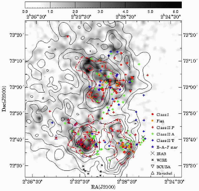
Figure 26: Surface distribution of the candidate YSOs, identified by infrared colors, overplotted on the visual extinction map of L1340, determined from star counts in the SDSS DR9 (Paper III). Black contours show ¹³CO integrated intensities, drawn at 0.6, 1.2, 1.8…K km s^-1, and red dash-dotted contour show the C¹⁸O contour at 0.35 K km s^-1. Meaning of the symbols are shown in the lower right corner.

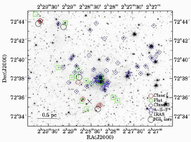
Figure 27: Surface distribution of the candidate YSOs and dense NH₃ cores in a $15.6\arcmin\times 12\arcmin$ area of L1340 A, plotted on the IRAC 3.6 µm image of the field.

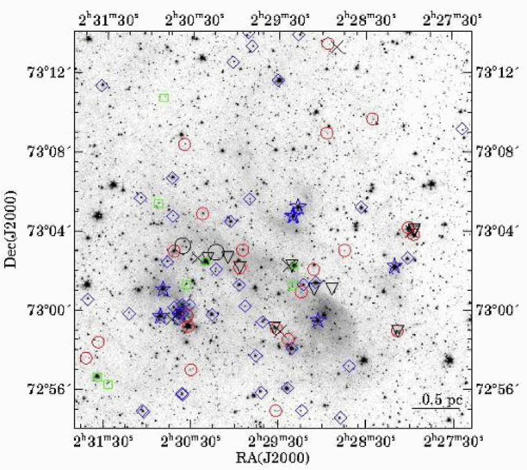
Figure 28: Surface distribution of the candidate YSOs and dense NH₃ cores in a $20\arcmin\times 20\arcmin$ area of L1340 B. Symbols are same as in Fig. 27, plus downward triangles mark submillimeter sources.

The positions of all candidate YSOs, identified by infrared color indices, are overplotted on the extinction map of the region, together with ¹³CO and C¹⁸O contours (from Paper I), in Fig. 26. More detailed maps of the central regions of the L1340 A, L1340 B, and L1340 C clumps are presented in Figs. 27, 28, and 29, respectively.

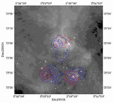
Figure 30: Left: Surface density distribution of the young stars, overplotted on the WISE 12-µm map of the cloud. Blue contours show the surface density of pre-main sequence stars, and red contours show that of the Class I + Flat SED sources. Each distribution was computed from the distances of the sixth nearest stars to the grid points. Right: The smoothed, composite surface density distribution of all candidate YSO classes, derived from the distance of the 20th nearest YSO to the grid points.

The surface distribution of the candidate YSOs reveals a rich population of young stars clustered over the clumps L1340 A, B, and C. We constructed surface density maps of the YSOs following the method described by Gutermuth et al. (2009). We determined the $r_{N}(i,j)$ distance of the $N$th nearest star at each (i,j) position of a uniform grid, and obtained the local surface density of YSOs at the grid point as $\rho(i,j)=N/\pi r_{N}^{2}(i,j)$. The surface density contour plot, shown in the left panel of Fig. 30, was constructed using a 30″  grid and $N=6$, and shows the surface densities of Class I+Flat (red dot-dashed contours) and Class II (blue solid contours) sources separately, overlaid on the WISE 12-µm image of L1340. The contour labels indicate the surface densities in star pc^-2 units. The YSO groups associated with the cloud clumps are apparent. Like the three clumps, the associated YSOs show diverse surface structures. The surface distribution in L1340 A suggests a west-to-east progression of star formation. Similarly, in L1340 C, Class I and Class II sources are apparently separated from each other. The largest clump L1340 B is associated with an extended, low surface density population. The right panel of Fig. 30 shows a composite surface density distribution of all YSO classes, derived at the same grid points, and using the distance of the 20th nearest YSO. The three clusterings, associated with the three clumps, remain apparent in the smoothed surface density map. The area of each YSO group and the number of stars within the surface density contour 2 stars pc^-2 are listed in Table 14.

5.1 Young Clusters in L1340

To find and characterise clusters in the YSO population of L1340 we examined the projected distances between the stars within the three groups seen in Fig. 30. Figure 31 shows the histograms of the nearest neighbor separations for the three groups, separately. The histograms of groups associated with L1340 A and L1340 C show peaks at short spacings, similarly to other nearby star-forming regions (Gutermuth et al., 2009). On the contrary, no preferred spacing range can be seen in the histogram of L1340 B. The median separations of the YSOs are 0.117 pc, 0.243 pc, and 0.141 pc in L1340 A, B, and C, respectively.

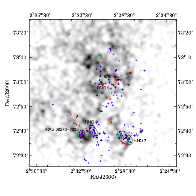
Figure 32: Distribution of candidate YSOs overplotted on the extinction map of L1340. Red symbols indicate Class I sources, green is for Flat, blue for Class II YSOs, and triangles indicate the submillimeter sources. Sources having a neighbor at a projected separation smaller than 0.15 pc are marked with underlying small black circles. Ellipses encircle the most prominent clusterings identified during this procedure.

Figure 32 show the YSO distribution overplotted on the extinction map, and the stars having a neighbor closer than 0.15 pc ($\approx$42″) are marked by underlying black dots. In L1340 A, 75 percent of the YSO population belong to this clustered subsystem, while 66 % of the YSOs in L1340 C and 34 % in L1340 B have neighbors within this distance. We identified four small clusters encircled by the overplotted ellipses. This criterion reveals 56 members of the RNO 7 cluster in L1340 A, including the K-band excess stars identified in the Omega-Cass data. The RNO 9 cluster in L1340 C consists of 22 Class II, three Flat, and one Class I sources, whereas six of the 12 members of the cluster associated with IRAS 02276+7225, are Class I/Flat sources. The only small clustering in clump B consists of eight stars, including the bright Class I source RNO 8. The coordinates and sizes of the clusters, identified by the nearest neighbor spacings, and the number of stars within them are listed in Table 15. The sizes are described by the major axis (a) and aspect ratio (AR) of the smallest ellipse encircling the members. The sampling of the members was not homogeneous, since part of L1340 A was not covered by the MIPS observations, whereas the IRAS 02276+7225 cluster is outside of the 4.5 µm  and 8 µm IRAC images. Moreover, eight members of the central core of RNO 7 comes from the Omega-Cass observations. For comparison, the last row of Table 15 lists the median values derived for the young cluster sample in our 1-kpc Galactic environment (Gutermuth et al., 2009).

5.2 YSO Distribution and the Cloud Structure

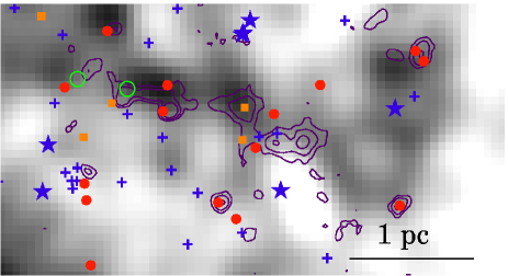
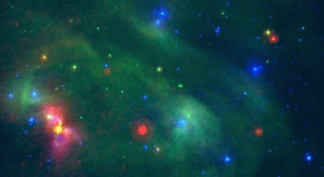
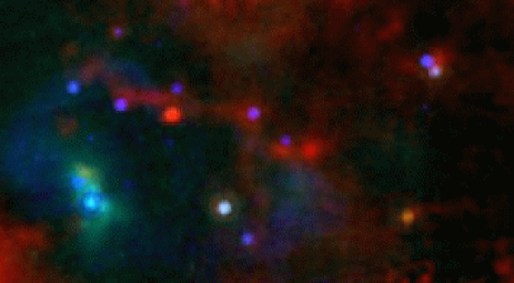
Figure 33: A multi-wavelength view of the central, $17.16\arcmin\times 9.3\arcmin$ area of the molecular clump L1340 B. The upper panel shows the positions of the B–A type stars (blue star symbols), Class 0/I infrared sources (red dots), Flat SED (orange squares), Class II YSOs, ammonia cores (Paper II, green circles) and the contours of 850-µm emission (purple contours, plotted at 30, 60, and 120 Jy beam^-1), overplotted on the extinction map. Class I sources associated with tenth-of-parsec scale density enhancements, and a bubble-like cavity, bordered by submm emission around an A-type star can be seen. The middle panel is a three-color image of the same area, composed of DSS2 blue (blue), Spitzer IRAC 8 µm (green), and MIPS 70 µm (red) images. It reveals a bow-shock like structure in the 8-µm emission around an A-type star, and the wispy structure of the diffuse 8-µm emission. Brightness and color diversities of the embedded stars reveal their diverse evolutionary stages and luminosities. Lower panel: Three-color image of the same region, composed of the MIPS 24 µm (blue), MIPS 70 µm (green), and SCUBA 800 µm (red) images. The infrared sources lined up along $\sim$ 2 pc long, cold filamentary structure.

The four small, compact clusters identified above comprise nearly half of the candidate YSOs. The distributed population consists of Class II stars scattered widely over low-extinction regions, and small groups of a few closely spaced YSOs. An example is the small aggregate marked by a red circle in Fig. 32, consisting of Class I, Flat, submillimeter, and strongly reddened Class II sources, and similar in angular size to the knots seen in the extinction map. To demonstrate the connection between the cloud structure and YSO distribution, we present in Fig. 33 a multi-wavelength view of L1340 B, revealing various aspects of interactions between the cloud and embedded stars. The upper panel of Fig 33 suggests that Class 0/I sources of L1340 B are associated with small-scale dust clumps. The morphology of this image suggests that the filamentary structure, detected at 850 µm, might have been created by past and present winds of the nearby young B- and A-type stars. The middle panel demonstrates the interactions of the intermediate-mass stars with the gas and dust, and reveals a diversity of the embedded YSOs. The lower panel reveals that a chain of Class 0/I/Flat sources and two ammonia cores (Paper II) are lined up along a ridge of 850 µm emission, starting with the Class 0 source J022808.60+725904.5 at the south-western side, and stretching over a projected length of some 3 pc to the Flat SED source 023042.36+730305.1 at the north-eastern end. The average separation of the protostars/bright knots along the submillimeter filament, $\sim$1.6′, corresponds to $\sim$0.4 pc at 825 pc.

Linear configurations in the distribution of protostars are thought to result from fragmentation of dense molecular filaments (e. g. Teixeira et al., 2006). The separation of protostars along the filament is of the order of the Jeans length. Temperatures and densities derived from the ammonia mapping of L1340 (from Paper II) suggest a Jeans length of $\sim 0.14$ pc for the dense cores of L1340. The wide separation of the protostars along the submillimeter filament of L1340 B, as well as the large average spacing of the nearest neighbors throughout the clump suggest higher temperature of the ambient medium. The NH₃ cores are probably the coldest regions of the cloud, embedded in a warmer gas, heated by the nearby B and A-type stars.

Another conspicuous linear feature is the J-shaped configuration of YSOs in L1340 C (the IRAS 02276+7225 cluster, Fig. 29). The average separation of the objects within that chain is 27.9″, corresponding to 0.11 pc at a distance of 825 pc. The total length of the chain is some 0.9 pc, suggesting that these stars have been formed from cores of $\sim 0.1$ pc in diameter. This coincides with the average size of the ammonia cores studied in Paper II, and is same as the Jeans length at $T_{\mathrm{kin}}\approx 12.5$ K and $n_{H_{2}}\approx 1.29\times 10^{4}$ cm^-3, resulted from the NH₃ observations. The cloud structure, underlying the observed distribution of the protostars, can be seen in the distribution of the cold dust, revealed by the Herschel SPIRE images (Fig. 7).

6 STAR FORMATION IN L1340

At a distance of 825 pc and a latitude of 11$\fdg$5 L1340 is situated some 160 pc above the Galactic plane, in a low-density outer region of the molecular disk of our Galaxy. (The Swan is floating on the surface of the Galactic molecular disk). The average hydrogen column densities of the three molecular clumps are about $2.5\times 10^{21}$ cm^-2, slightly lower than the mean column density of $4.38\times 10^{21}$ cm^-2, obtained by Lundquist et al. (2015) for IM SFRs in the outer Galaxy. The extinction map of L1340 (Paper III) reveals a shallow molecular cloud, spotted with dense knots of a few arcminutes ($\sim 0.5$ pc) characteristic size. YSOs are grouped on similar angular scales, and Class 0/I–Flat sources appear closely associated with extinction knots (see Fig. 33), suggesting that star formation occurs in small groups, consisting of a few stars, and scattered over the surface of the cloud. The most massive star in L1340 is an optically visible B4-type star of some 5 M_☉, whereas the YSOs revealed by our present survey are in the $0.07\lesssim M/M_{\sun}\lesssim 2.5$ mass interval.

The number of embedded sources, and their ratio to the more evolved pre-main sequence stars in a star-forming region is an indicator of evolutionary state. Myers (2012) established relations between Class II/Class I number ratios, as well as ages and birthrates of young stellar clusters, assuming a constant protostellar birthrate. The Class II/Class I ratio (Table 14) suggests an age of 1 million years and a birthrate of 200–300 protostars/Myr. The three clumps of L1340 differ from each other in several respects. The effects of young intermediate-mass stars on the environment are conspicuous in L1340 B. The wispy structure of the 8-µm emission, the bow-shock like structure associated with an A2-type star, and the double-peaked CO lines at the positions of the Planck Cold Clumps (Wu et al., 2012) associated with L1340, suggest violent swirling of the gas in this region. The low surface density of YSOs, compared to the other clumps of the cloud, indicates that the prestellar gas in L1340 B had higher temperature and lower density than in L1340 A and L1340 C, due to the heating from the ambient B-type stars. The higher proportion of protostars in L1340 B (NII/(NI+NFlat)=1.47) suggests that the average age of the YSO sample is lower in this clump than in the others. Star-forming regions like L1340 B are probably more transient structures than centrally condensed young embedded clusters. Pfalzner et al. (2015) have found that only clusters and associations with initial central surface densities exceeding a few 1000 M_☉ pc^-2 will be detected as clusters at ages longer than 5 Myr.

Assuming an average mass of 0.5 M_☉ for each candidate YSO, and including the intermediate-mass stars, discussed in Paper III, we find the star formation efficiencies (SFE = $M_{star}/(M_{star}+M_{cloud}$) listed in Table 14 for the three clumps of L1340. It can be seen that while some 17% of the gas turned into star in L1340 A, the SFE is only 3% for L1340 B and also for the whole cloud. The actual SFEs are probably somewhat higher, since the low-mass diskless YSO population of L1340 is still unknown.

6.1 Comparison with Other Star-Forming Regions

Comparison of our target cloud with IM SFRs, located in similar environments, may help to understand the interstellar processes, leading to star formation near the outer boundaries of the Galactic molecular disk. The short expected lifetime of L1340 (probably $\ll 5$ Myr) suggests that similar star-forming regions may be rare in our Galactic neighborhood. A sample 50 IMSFRs, studied by Arvidsson et al. (2010), contains objects similar in stellar content and total mass to L1340. Most of them are, however, more distant and thus their detailed structures are still unrevealed. The Spitzer sample of young clusters in our Galactic neighborhood (SSYSC, Gutermuth et al., 2009) also contains several IMSFRs. Comparison of our results with several properties of this sample of young clusters is shown in Table 15. It suggests that the clusters, identified in the YSO population of L1340 are similar in size, shape, and stellar content to the SSYSC average. The distribution of the projected YSO separations, however, suggests that the mode of star formation in L1340 B is quite atypical. The median nearest neighbor separations are significantly smaller in each of the SSYSC clusters than in L1340 B. Another atypical feature of L1340 is that conspicuous YSO groups are being formed in the smaller clumps, whereas the largest clump, associated with the highest luminosity stars of the region, has a fragmented structure, associated with tiny groups of YSOs, scattered over the area of the clump.

A few IM SFRs in our 1-kpc Galactic environment are also located at latitudes around 10° or higher, and are apparently not associated with giant molecular clouds. Well-known examples are NGC 7023 and NGC 7129, both located more than 100 pc above the Galactic plane, and forming small clusters with the brightest stars of B3 type. These regions may have star-forming histories similar to L1340. Expanding supershells could create conditions of star formation intermediate Galactic latitudes. Apparently none of these star-forming regions are associated with supershells, thus some other process, such as infall of high velocity clouds, or Kelvin–Helmholtz instabilities arising at the shearing surface between gas layers of different velocities might have compressed the gas.

7 Conclusions

We identified some 250 candidate YSOs associated with the moderate-mass ($\sim 3700$ M_☉  Paper III) molecular cloud L1340, based on Spitzer, AllWISE mid-infrared, and Omega-Cass near-infrared data, using various published color criteria. Supplemented with our measurements on the Herschel PACS 100 µm and 160 µm images and publicly available photometric data we constructed spectral energy distributions, and classified 8 candidate Class 0, 37 Class I, 27 Flat SED, and 170 Class II sources. Based on the SEDs we derived extinctions and spectral types for the Class II sources, and plotted them onto the Hertzsprung–Russell diagram. The HRD suggests a mass interval of 0.07–2.5 M_☉ for the CTTS of our sample.

We identified new Herbig–Haro objects, associated with the Class 0 protostar SSTSL2 022808.60+725904.5 in the Spitzer images. The Spitzer data reveal that the bright IRAS source 02249+7230 is a binary protostar associated with Herbig–Haro objects. The Spitzer data also suggest that the probable driving source of HH 488 is a Class 0 protostar, SSTSL2 J022820.81+723500.5. The projected length of HH 488 is some 1.3 pc.

The Omega-Cass JHK data resulted in 8 new candidate members of RNO 7, and revealed a close companion of its brighest member, IRAS 02236+7224. The Spitzer 8-µm image revealed two further wide companions of this intermediate-mass T Tauri star.

The surface density distribution of young stellar objects shows three groups, associated with the three major molecular clumps of L1340, each consisting of $\lesssim 100$ members, including both pre-main sequence stars and embedded protostars. Based on the distribution of nearest neighbor separations we identified four small clusters in the cloud, the RNO 7 cluster in L1340 A, RNO 8 in L1340 B, and RNO 9 and IRAS 02276+7225 in L1340 C. Filamentary configurations of the protostars follow the distribution of the cold dust, traced by SCUBA and Herschel observations. The efficiency of the star formation in L1340 is some 3 %. Our results demonstrate that L1340 is a prolific star-forming region of our Galactic environment in which several specific properties of the intermediate-mass mode of star formation can be studied in detail. The distribution of dense gas and YSOs suggest that star-forming regions like L1340 are short-lived, transient objects.

Appendix A UBVR_CI_CJHK_s PHOTOMETRIC DATA OF THE CLASS II YOUNG STELLAR OBJECTS

We list UBVR_CI_C magnitudes, transformed from the SDSS data, and 2MASS JHK_s magnitudes of the color-selected candidate Class II young stars associated with L1340 in Table A1, excluded the H$\alpha$ emission stars, whose data are given in Paper III.

Figure 1: Outlines of the Spitzer IRAC (3.6 and 5.8 µm: blue solid line, 4.5 and 8.0 µm: red dash-dotted line), MIPS 24 µm (orange, dash-three dots), MIPS 70 µm (black dash-dotted line) observations, overplotted on the DSS2 red image of the region, one square degree in area. Both the lowest contour and the increment of the overlaid ¹³CO integrated intensity map are 0.5 K km s^-1.

Figure 3: WISE 4.6 $\mu$m (blue), 12 $\mu$m (green), and 22 $\mu$m (red) composite image of L1340. The size of the image is 1 square degree, and is centered on RA(J2000) = 37$\fdg$625, Dec(J2000) = +72$\fdg$933. Small groups of 22-µm sources point to the three star-forming clumps of L1340. The extended 12 µm emission (the Swan nebula) is excited by the B and A type stars associated with L1340 B. The annotated objects are the most striking signposts of low-mass star formation: IRAS 02224+7227 is a FUor-like star (Kun et al., 2014), IRAS 02249+7230 is a protostellar source exciting HH 489, RNO 7, RNO 8, and RNO 9 are nebulous, partially embedded stellar groups, and V1180 Cas is an eruptive star (Kun et al., 2011).

Figure 6: Three-color image of L1340 B, the Swan Nebula, composed of Spitzer IRAC 4.5 µm (blue), 8.0 µm (green) and MIPS 24 µm (red) images.

Figure 9: Spectral energy distributions of Class I YSOs. Open circles show the SDSS, 2MASS, and WISE data, and triangles indicate the Spitzer data. Crosses are for Akari FIS data, diamonds show the Herschel data points, and squares indicate SCUBA submillimeter fluxes.

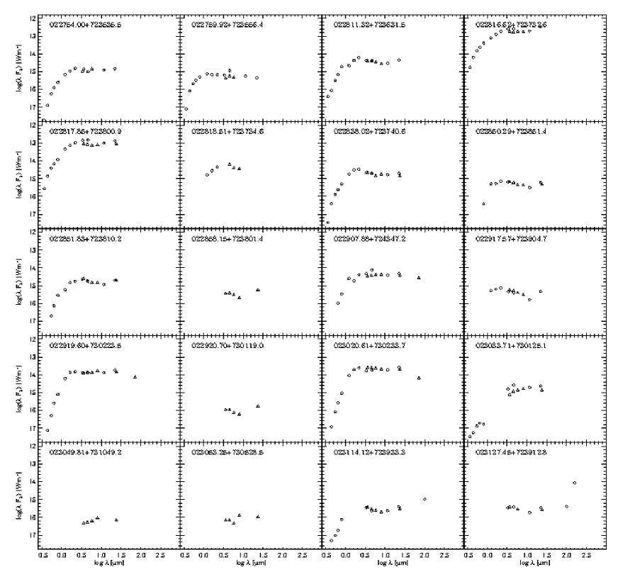
Figure 10: SEDs of the Flat SED infrared sources. Symbols are same as in Fig. 9.

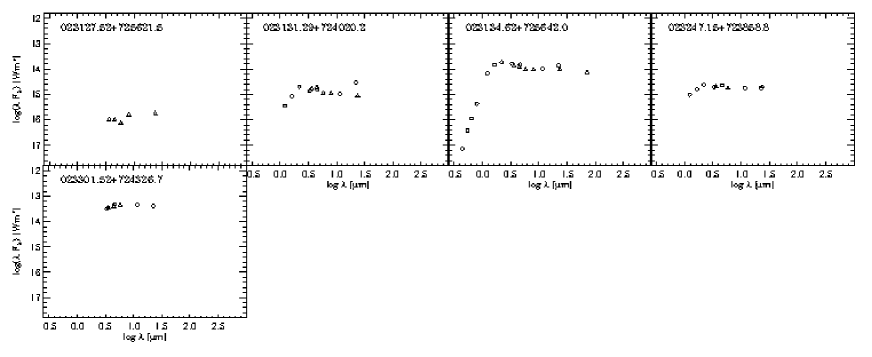
Figure 10: SEDs of the Flat SED infrared sources (continued).

Figure 11: SEDs of the Class II candidate YSOs (continued).

  

  

Figure 20: Three-color image, composed of the IRAC 3.6 µm (blue), 4.5 µm (green), and 8 µm (red) images of the environment of the candidate Class 0 protostar SSTSL2 J022931.98+725912.4. Notice the color difference between the eastern and western nebulosities.

Figure 31: Histograms of the nearest neighbor separations for the three clumps of L1340.

Table 1: SEIP SSTSL2 Fluxes and uncertainties of Class 0/I sources in L1340

No.	SSTSL2	$F_{3.6}$	$F_{4.5}$	$F_{5.8}$	$F_{8.0}$	$F_{24}$	$F_{70}$
		(mJy)	(mJy)	(mJy)	(mJy)	(mJy)	(mJy)
1	022756.91+730354.4	1.915 $\pm$ 0.005	3.782 $\pm$ 0.007	5.412 $\pm$ 0.016	6.104 $\pm$ 0.013	73.620 $\pm$ 0.164	828.038 $\pm$ 58.375
2	022800.65+730415.2	14.510 $\pm$ 0.014	25.430 $\pm$ 0.018	40.200 $\pm$ 0.044	67.940 $\pm$ 0.035	289.700 $\pm$ 0.263	404.928 $\pm$ 28.732
3	022808.60+725904.5	1.774 $\pm$ 0.005	2.873 $\pm$ 0.007	2.982 $\pm$ 0.013	1.888 $\pm$ 0.010	1.775 $\pm$ 0.132	596.200 $\pm$ 16.900
4	022818.51+723506.2	1.586 $\pm$ 0.004	6.086 $\pm$ 0.023	8.608 $\pm$ 0.020	9.509 $\pm$ 0.010	$\cdots$	$\cdots$
5	022820.81+723500.5	0.251 $\pm$ 0.001	2.019 $\pm$ 0.015	4.189 $\pm$ 0.014	8.067 $\pm$ 0.025	$\cdots$	$\cdots$
6	022825.07+730945.6	0.150 $\pm$ 0.002	0.179 $\pm$ 0.002	0.197 $\pm$ 0.007	0.842 $\pm$ 0.011	22.590 $\pm$ 0.135	43.500 $\pm$ 11.100
7	022842.57+723544.3	11.560 $\pm$ 0.010	19.330 $\pm$ 0.036	27.290 $\pm$ 0.034	28.610 $\pm$ 0.026	$\cdots$	$\cdots$
8	022844.40+723533.5	3.473 $\pm$ 0.005	4.359 $\pm$ 0.024	7.668 $\pm$ 0.019	7.259 $\pm$ 0.018	$\cdots$	$\cdots$
9	022844.71+730308.5	0.110 $\pm$ 0.002	0.135 $\pm$ 0.002	0.155 $\pm$ 0.007	0.284 $\pm$ 0.012	0.935 $\pm$ 0.121	$\cdots$
10	022849.44+723731.6	0.035 $\pm$ 0.001	0.079 $\pm$ 0.002	0.105 $\pm$ 0.005	$<$ 0.023	$<$0.491	$\cdots$
11	022855.69+731333.1	0.039 $\pm$ 0.001	0.063 $\pm$ 0.002	0.075 $\pm$ 0.006	0.083 $\pm$ 0.008	0.858 $\pm$ 0.132	$\cdots$
12	022856.61+730903.2	0.108 $\pm$ 0.002	0.146 $\pm$ 0.002	0.212 $\pm$ 0.006	0.337 $\pm$ 0.007	2.936 $\pm$ 0.135	$\cdots$
13	022906.09+730210.5	0.022 $\pm$ 0.001	0.030 $\pm$ 0.002	0.039 $\pm$ 0.004	0.063 $\pm$ 0.008	0.657 $\pm$ 0.124	$\cdots$
14	022914.62+730102.8	0.063 $\pm$ 0.001	0.081 $\pm$ 0.002	$\cdots$	0.381 $\pm$ 0.007	1.270 $\pm$ 0.137	$\cdots$
15	022918.25+724754.0	0.081 $\pm$ 0.001	0.097 $\pm$ 0.002	0.087 $\pm$ 0.006	0.074 $\pm$ 0.008	3.509 $\pm$ 0.127	64.600 $\pm$ 9.80
16	022931.98+725912.4	0.959 $\pm$ 0.003	1.755 $\pm$ 0.005	1.699 $\pm$ 0.010	1.159 $\pm$ 0.009	211.700 $\pm$ 0.218	1949.471 $\pm$ 136.77
17	022932.31+725503.2	0.226 $\pm$ 0.002	0.274 $\pm$ 0.002	0.419 $\pm$ 0.006	0.956 $\pm$ 0.009	5.341 $\pm$ 0.134	$\cdots$
18	022943.01+724359.6	$\cdots$	2.118 $\pm$ 0.005	3.482 $\pm$ 0.005	6.541 $\pm$ 0.015	$<$ 0.659	$\cdots$
19	022943.64+724358.6	2.316 $\pm$ 0.004	7.394 $\pm$ 0.012	13.270 $\pm$ 0.024	19.350 $\pm$ 0.021	375.200 $\pm$ 0.250	2496.581 $\pm$  175.06
20	022949.62+725326.1	0.238 $\pm$ 0.002	0.428 $\pm$ 0.003	0.622 $\pm$ 0.007	1.286 $\pm$ 0.010	53.000 $\pm$ 0.153	103.044 $\pm$  7.602
21	022955.10+730309.1	1.703 $\pm$ 0.005	3.281 $\pm$ 0.008	6.332 $\pm$ 0.018	14.200 $\pm$ 0.018	58.580 $\pm$ 0.165	51.500 $\pm$ 21.000
22	022956.90+730217.0	$\cdots$	$\cdots$	$\cdots$	$\cdots$	$\cdots$	262.0 $\pm$ 36.6
23	023022.78+730459.0	1.137 $\pm$ 0.004	1.790 $\pm$ 0.006	2.709 $\pm$ 0.012	3.747 $\pm$ 0.013	24.220 $\pm$ 0.155	69.852 $\pm$ 5.871
24	023030.42+725706.7	0.084 $\pm$ 0.001	0.108 $\pm$ 0.002	0.156 $\pm$ 0.005	0.293 $\pm$ 0.008	2.228 $\pm$ 0.126	$\cdots$
25	023032.44+725918.0	79.412 $\pm$ 3.192	115.791 $\pm$ 4.498	215.566 $\pm$ 7.104	528.239 $\pm$ 18.993	2069.692 $\pm$ 82.791	1876.886 $\pm$ 132.659
26	023035.51+730828.2	0.227 $\pm$ 0.002	0.466 $\pm$ 0.003	0.753 $\pm$ 0.008	1.187 $\pm$ 0.010	3.066 $\pm$ 0.113	$\cdots$
27	023042.36+730305.1	4.773 $\pm$ 0.009	13.510 $\pm$ 0.016	24.490 $\pm$ 0.034	28.800 $\pm$ 0.024	117.100 $\pm$ 0.180	484.031 $\pm$ 34.168
28	023127.34+724012.9	2.280 $\pm$ 0.072	5.119 $\pm$ 0.353	10.224 $\pm$ 0.313	15.729 $\pm$ 0.518	101.771 $\pm$ 4.074	663.806 $\pm$ 46.801
29	023134.23+725829.1	0.057 $\pm$ 0.001	0.090 $\pm$ 0.001	0.119 $\pm$ 0.005	0.075 $\pm$ 0.007	0.782 $\pm$ 0.119	$\cdots$
30	023142.50+725740.4	0.049 $\pm$ 0.001	0.069 $\pm$ 0.002	0.076 $\pm$ 0.005	0.355 $\pm$ 0.010	0.808 $\pm$ 0.123	$\cdots$
31	023146.58+723729.4	$\cdots$	$\cdots$	0.256 $\pm$ 0.006	$\cdots$	3.952 $\pm$ 0.128	$\cdots$
32	023203.42+724131.7	0.062 $\pm$ 0.001	0.177 $\pm$ 0.002	0.417 $\pm$ 0.008	0.930 $\pm$ 0.012	3.437 $\pm$ 0.112	$\cdots$
33	023207.96+723759.3	0.784 $\pm$ 0.003	$\cdots$	3.255 $\pm$ 0.013	$\cdots$	26.570 $\pm$ 0.146	162.799 $\pm$ 11.629
34	023225.98+724020.1	$\cdots$	$\cdots$	9.834 $\pm$ 0.021	$\cdots$	79.120 $\pm$ 0.163	626.957 $\pm$ 44.163
35	023226.35+723919.4	2.839 $\pm$ 0.005	$\cdots$	1.752 $\pm$ 0.009	$\cdots$	72.926 $\pm$ 1.888	375.855 $\pm$ 27.889
36	023227.64+723841.4	0.693 $\pm$ 0.022	$\cdots$	0.847 $\pm$ 0.033	$\cdots$	17.613 $\pm$ 0.715	378.511 $\pm$ 27.082
37	023232.00+723827.5	4.784 $\pm$ 0.006	$\cdots$	13.880 $\pm$ 0.025	$\cdots$	57.910 $\pm$ 0.124	343.451 $\pm$ 24.445
38	023237.90+723940.7	0.094 $\pm$ 0.001	$\cdots$	0.543 $\pm$ 0.007	$\cdots$	$<$ 0.361	$\cdots$
39	023248.83+724635.4	0.305 $\pm$ 0.002	0.251 $\pm$ 0.002	0.226 $\pm$ 0.007	2.142 $\pm$  0.009	3.936 $\pm$ 0.138	$\cdots$
40	023256.14+724605.3	1.338 $\pm$ 0.003	1.697 $\pm$ 0.004	1.639 $\pm$ 0.010	1.428 $\pm$ 0.008	57.310 $\pm$ 0.147	847.044 $\pm$ 59.580
41	023302.41+724331.2	5.987 $\pm$ 0.007	14.790 $\pm$ 0.012	27.930 $\pm$ 0.035	57.890 $\pm$ 0.033	530.100 $\pm$ 0.265	2281.543 $\pm$ 160.168
42	023330.92+724800.3	0.162 $\pm$ 0.002	0.248 $\pm$ 0.002	0.246 $\pm$ 0.007	0.297 $\pm$ 0.009	11.950 $\pm$ 0.128	$\cdots$
43	023340.83+731950.8	6.178 $\pm$ 0.007	11.280 $\pm$ 0.010	16.950 $\pm$ 0.029	24.350 $\pm$ 0.031	$\cdots$	$\cdots$
44	023432.66+724057.2	0.243 $\pm$ 0.002	$\cdots$	0.636 $\pm$ 0.007	$\cdots$	3.180 $\pm$ 0.117	$\cdots$
45	023532.06+724922.6	0.079 $\pm$ 0.001	0.098 $\pm$ 0.002	0.101 $\pm$ 0.006	0.138 $\pm$ 0.008	2.856 $\pm$ 0.133	$\cdots$

Table 2: SEIP SSTSL2 fluxes and uncertainties of Flat SED sources in L1340

No.	SSTSL2	$F_{3.6}$	$F_{4.5}$	$F_{5.8}$	$F_{8.0}$	$F_{24}$	$F_{70}$
		(mJy)	(mJy)	(mJy)	(mJy)	(mJy)	(mJy)
1	022754.00+723535.5	1.744 $\pm$ 0.004	1.766 $\pm$ 0.020	2.957 $\pm$ 0.012	0.245 $\pm$ 0.018	$\cdots$	$\cdots$
2	022759.92+723556.4	0.523 $\pm$ 0.026	0.859 $\pm$ 0.060	0.980 $\pm$ 0.032	$\cdots$	$\cdots$
3	022811.32+723631.5	4.896 $\pm$ 0.086	6.002 $\pm$ 0.011	6.895 $\pm$ 0.011	7.715 $\pm$ 0.014	$\cdots$	$\cdots$
4	022816.62+723732.6	219.545 $\pm$ 28.270	268.500 $\pm$ 0.135	361.400 $\pm$ 0.124	374.611 $\pm$ 11.495	$\cdots$	$\cdots$
5	022817.85+723800.9	92.280 $\pm$ 0.027	108.000 $\pm$ 0.056	140.700 $\pm$ 0.078	219.498 $\pm$ 6.839	857.300 $\pm$ 0.612	$\cdots$
6	022818.51+723734.6	$\cdots$	9.617 $\pm$ 0.021	8.287 $\pm$ 0.019	9.695 $\pm$ 0.015	$\cdots$	$\cdots$
7	022838.02+723740.6	2.805 $\pm$ 0.005	2.963 $\pm$ 0.006	3.217 $\pm$ 0.012	5.370 $\pm$ 0.012	12.010 $\pm$ 0.516	$\cdots$
8	022850.36+723851.2	0.822 $\pm$ 0.003	0.883 $\pm$ 0.004	0.897 $\pm$ 0.008	1.218 $\pm$ 0.009	4.005 $\pm$ 0.180	$\cdots$
9	022851.83+723810.2	2.934 $\pm$ 0.005	3.027 $\pm$ 0.007	2.980 $\pm$ 0.012	3.900 $\pm$ 0.012	16.730 $\pm$ 0.215	$\cdots$
10	022858.15+723801.4	0.461 $\pm$ 0.002	0.607 $\pm$ 0.003	0.627 $\pm$ 0.007	0.551 $\pm$ 0.009	4.872 $\pm$ 0.185	$\cdots$
11	022907.88+724347.2	3.938 $\pm$ 0.006	5.972 $\pm$ 0.010	8.489 $\pm$ 0.020	11.680 $\pm$ 0.017	30.940 $\pm$ 0.142	66.994 $\pm$ 5.117
12	022917.57+723904.7	0.735 $\pm$ 0.003	0.803 $\pm$ 0.005	0.818 $\pm$ 0.008	0.853 $\pm$ 0.010	$\cdots$	$\cdots$
13	022919.60+730223.5	15.980 $\pm$ 0.014	21.360 $\pm$ 0.018	26.930 $\pm$ 0.036	46.410 $\pm$ 0.029	131.700 $\pm$ 0.180	181.009 $\pm$ 20.0
14	022920.70+730119.0	0.137 $\pm$ 0.002	0.171 $\pm$ 0.002	0.156 $\pm$ 0.005	0.169 $\pm$ 0.007	1.491 $\pm$ 0.128	$\cdots$
15	022950.37+724441.4	0.069 $\pm$ 0.001	0.092 $\pm$ 0.002	0.163 $\pm$ 0.005	0.341 $\pm$ 0.009	0.877 $\pm$ 0.120	$\cdots$
16	023020.61+730233.7	30.700 $\pm$ 0.023	35.390 $\pm$ 0.029	47.510 $\pm$ 0.048	61.830 $\pm$ 0.034	174.500 $\pm$ 0.212	162.696 $\pm$ 11.950
17	022920.70+730119.0	0.137 $\pm$ 0.002	0.171 $\pm$ 0.002	0.156 $\pm$ 0.005	0.169 $\pm$ 0.007	1.491 $\pm$ 0.128
18	023033.71+730125.1	0.957 $\pm$ 0.004	1.813 $\pm$ 0.005	2.940 $\pm$ 0.013	4.755 $\pm$ 0.012	11.630 $\pm$ 0.134	$\cdots$
19	023049.81+731049.2	0.059 $\pm$ 0.002	0.084 $\pm$ 0.002	0.128 $\pm$ 0.006	0.255 $\pm$ 0.007	0.581 $\pm$ 0.100	$\cdots$
20	023053.25+730528.5	0.087 $\pm$ 0.001	0.109 $\pm$ 0.002	0.091 $\pm$ 0.005	0.366 $\pm$ 0.009	0.871 $\pm$ 0.123	$\cdots$
21	023114.12+723933.3	0.480 $\pm$ 0.002	0.462 $\pm$ 0.004	0.482 $\pm$ 0.007	0.568 $\pm$ 0.019	2.432 $\pm$ 0.125	$\cdots$
22	023127.45+723912.8	0.488 $\pm$ 0.002	$\cdots$	0.592 $\pm$ 0.007	$\cdots$	2.234 $\pm$ 0.132	$\cdots$
23	023127.52+725621.5	0.133 $\pm$ 0.001	0.157 $\pm$ 0.002	0.150 $\pm$ 0.005	0.447 $\pm$ 0.009	1.513 $\pm$ 0.123	$\cdots$
24	023134.62+725642.0	16.900 $\pm$ 0.012	18.840 $\pm$ 0.013	19.710 $\pm$ 0.031	28.240 $\pm$ 0.032	82.320 $\pm$ 0.177	180.167 $\pm$ 12.921
25	023247.15+723858.8	2.079 $\pm$ 0.004	$\cdots$	2.887 $\pm$ 0.005	$\cdots$	17.390 $\pm$ 0.126	$\cdots$
26	023254.71+724257.9	0.077 $\pm$ 0.001	0.132 $\pm$ 0.002	0.211 $\pm$ 0.005	0.378 $\pm$  0.009	1.131 $\pm$ 0.104	$\cdots$
27	023301.52+724326.7	43.430 $\pm$ 0.018	63.980 $\pm$ 0.025	91.940 $\pm$ 0.064	$\cdots$	$<$0.325	$\cdots$

Table 3: SEIP SSTSL2 Fluxes and uncertainties of of Class II sources

SSTSL2	$F_{3.6}$	$F_{4.5}$	$F_{5.8}$	$F_{8.0}$	$F_{24}$	$F_{70}$
	(mJy)	(mJy)	(mJy)	(mJy)	(mJy)	(mJy)
022638.02+730457.5	3.517 $\pm$ 0.147	3.965 $\pm$ 0.009	4.335 $\pm$ 0.015	5.878 $\pm$ 0.015	7.710 $\pm$ 0.116	36.198 $\pm$ 3.178
022654.73+724040.8	1.552 $\pm$ 0.004	1.012 $\pm$ 0.004	0.527 $\pm$ 0.007	0.461 $\pm$ 0.010	4.301 $\pm$ 0.179	$\cdots$
022659.03+725716.0	1.477 $\pm$ 0.005	1.156 $\pm$ 0.003	0.921 $\pm$ 0.006	0.739 $\pm$ 0.009	5.040 $\pm$ 0.115	$\cdots$
022659.08+724016.6	0.966 $\pm$ 0.003	0.815 $\pm$ 0.004	0.667 $\pm$ 0.007	0.893 $\pm$ 0.009	1.221 $\pm$ 0.200	$\cdots$
022659.35+725714.2	1.581 $\pm$ 0.005	1.204 $\pm$ 0.003	0.981 $\pm$ 0.006	1.098 $\pm$ 0.009	9.337 $\pm$ 0.117	$\cdots$
022700.34+724743.8	2.571 $\pm$ 0.005	1.920 $\pm$ 0.006	1.573 $\pm$ 0.009	2.136 $\pm$ 0.010	8.947 $\pm$ 0.126	$\cdots$
022702.11+724329.0	2.061 $\pm$ 0.004	1.617 $\pm$ 0.006	1.043 $\pm$ 0.008	0.968 $\pm$ 0.011	2.460 $\pm$ 0.123	$\cdots$
022703.17+723952.9	1.172 $\pm$ 0.003	1.177 $\pm$ 0.005	0.794 $\pm$ 0.007	1.192 $\pm$ 0.009	2.206 $\pm$ 0.179	$\cdots$
022705.53+724116.7	169.100 $\pm$ 5.4640	131.753 $\pm$ 5.460	125.8 $\pm$ 4.2880	147.395 $\pm$ 4.713	197.200 $\pm$ 0.3030	$\cdots$
022706.29+724011.1	1.918 $\pm$ 0.070	1.344 $\pm$ 0.044	0.878 $\pm$ 0.008	0.912 $\pm$ 0.009	2.466 $\pm$ 0.181	$\cdots$

Note. — Table 3 is published in its entirety in the electronic edition of the Astrophysical Journal. A portion is shown here for guidance regarding its form and content.

Table 4: Herschel PACS point sources associated with candidate Spitzer YSOs in L1340 C

No.	SSTSL2	Fitted RA	Fitted Dec	$F_{100}$	$dF_{100}$	$F_{160}$	$dF_{160}$
		(deg)	(deg)	(mJy)	(mJy)	(mJy)	(mJy)
1	022907.88+724347.2	37.28481	72.73014	349.372	$\cdots$	1073.854	$\cdots$
2	022943.64+724358.6	37.43316	72.73337	9899.194	$\cdots$	11999.27	$\cdots$
3	023114.12+723933.3	37.82169	72.66068	34.923	353.948	$\cdots$	$\cdots$
4	023127.45+723912.8	37.87831	72.65379	13.773	101.163	0474.558	38.295
5	023127.34+724013.0	37.86170	72.67144	918.261	124.522	1652.396	155.898
6	023146.58+723729.4	37.93610	72.62243	16.760	57.825	0342.640	66.379
7	023203.42+724131.7	38.01794	72.68809	0.424	182.745	0101.090	62.318
8	023207.96+723759.3	38.03459	72.63372	258.719	205.061	0500.088	85.020
9	023225.98+724020.1	38.11119	72.67221	879.202	47.523	1712.686	87.426
10	023226.35+723919.4	38.10945	72.65580	488.341	196.238	2403.526	376.658
11	023227.64+723841.4	38.11722	72.64574	1118.237	187.990	2461.969	379.767
12	023232.00+723827.5	38.13490	72.64143	639.157	122.241	2462.245	379.627
13	023237.90+723940.7	38.15584	72.66280	22.780	114.644	264.833	156.138
14	023247.15+723858.8	38.19769	72.65025	37.372	194.085	175.280	226.861
15	023248.83+724635.4	38.20506	72.77680	75.233	51.971	$\cdots$	$\cdots$
16	023254.71+724257.9	38.22334	72.71396	7.888	142.752	$\cdots$	$\cdots$
17	023256.14+724605.3	38.23558	72.76854	1798.065	105.467	2059.933	84.941
18	023302.41+724331.2	38.26159	72.72580	2621.677	155.127	2801.787	100.030
19	023331.04+724800.8	38.38035	72.80073	119.108	168.020	470.005	69.517
20	023432.66+724057.2	38.63831	72.68040	23.361	173.174	$\cdots$	$\cdots$

Table 5: Spitzer sources of Class 0/I SED: Associated objects

SSTSL2	SDSS DR9 J	2MASS	AllWISE J	IRAS	Akari FIS	JCMTSF J	Other
022756.91+730354.4	$\cdots$	02275695+7303542	022756.94+730354.6	$\cdots$	0227565+730402	022756.6+730404	$\cdots$
022800.65+730415.2	022800.91+730415.4g	02280074+7304154	022800.60+730415.4	$\cdots$	$\cdots$	$\cdots$	$\cdots$
022808.60+725904.5	$\cdots$	$\cdots$	022808.59+725904.0	$\cdots$	0228071+725858	022808.4+725902	$\cdots$
022818.51+723506.2	$\cdots$	02281842+7235061	022818.46+723506.3	$\cdots$	$\cdots$	$\cdots$	$\cdots$
022820.81+723500.5	$\cdots$	$\cdots$	022820.76+723500.6	$\cdots$	0228201+723504	$\cdots$
022825.07+730945.6	$\cdots$	$\cdots$	022825.06+730945.7	$\cdots$	$\cdots$	$\cdots$	$\cdots$
022842.57+723544.3	022842.55+723544.5g	02284255+7235444	022842.54+723544.5	$\cdots$	$\cdots$	$\cdots$	$\cdots$
022844.40+723533.5	022844.40+723532.9g	02284443+7235332	022844.39+723533.6	$\cdots$	$\cdots$	$\cdots$	$\cdots$
022844.71+730308.5	$\cdots$	$\cdots$	022844.66+730308.6	$\cdots$	$\cdots$	$\cdots$	$\cdots$
022849.44+723731.6	$\cdots$	$\cdots$	022849.40+723732.5	$\cdots$	$\cdots$	$\cdots$	$\cdots$
022855.69+731333.1	$\cdots$	$\cdots$	022855.89+731333.1	02240+7259	$\cdots$	$\cdots$	$\cdots$
022856.61+730903.2	$\cdots$	$\cdots$	022856.62+730903.1	$\cdots$	$\cdots$	$\cdots$	$\cdots$
022906.09+730210.5	$\cdots$	$\cdots$	$\cdots$	$\cdots$	$\cdots$	$\cdots$	$\cdots$
022914.62+730102.8	$\cdots$	$\cdots$	022914.67+725405.5	$\cdots$	$\cdots$	$\cdots$	$\cdots$
022918.25+724754.0	$\cdots$	$\cdots$	$\cdots$	$\cdots$	$\cdots$	$\cdots$	$\cdots$
022931.98+725912.4	$\cdots$	02293228+7259130	022932.05+725913.0	02248+7245	0229320+725911	022933.2+725914
022932.31+725503.2	022932.32+725503.3*	$\cdots$	022932.30+725503.2	$\cdots$	$\cdots$	$\cdots$	$\cdots$
022943.01+724359.6	022943.09+724359.7	$\cdots$	022943.58+724358.6	02249+7230	$\cdots$	$\cdots$	HH 489S
022943.64+724358.6	022949.66+725325.8	$\cdots$	022943.58+724358.6	02249+7230	$\cdots$	$\cdots$	HH 489S
022949.62+725326.1	$\cdots$	$\cdots$	022949.65+725326.3	$\cdots$	$\cdots$	$\cdots$	$\cdots$
022955.10+730309.1	$\cdots$	02295507+7303094	022955.11+730309.4	$\cdots$	$\cdots$	$\cdots$	$\cdots$
022956.90+730217.0	$\cdots$	$\cdots$	022957.34+730211.1	$\cdots$	$\cdots$	022956.9+730217
023022.78+730459.0	$\cdots$	$\cdots$	023022.79+730459.0	$\cdots$	$\cdots$	022956.9+730217
023030.42+725706.7	$\cdots$	$\cdots$	023030.34+725707.0	$\cdots$	$\cdots$	$\cdots$	$\cdots$
023032.44+725918.0	023032.47+725917.7	02303247+7259177	023032.46+725917.8	02259+7246	$\cdots$	$\cdots$	RNO 8
023035.51+730828.2	$\cdots$	$\cdots$	023035.52+730828.5	$\cdots$	$\cdots$	$\cdots$	$\cdots$
023042.36+730305.1	$\cdots$	02304238+7303051	023042.36+730305.2	$\cdots$	$\cdots$	$\cdots$	$\cdots$
023127.34+724012.9	$\cdots$	02312734+7240130	023127.20+724015.5	02267+7226	0231270+724015	$\cdots$	$\cdots$
023134.23+725829.1	$\cdots$	$\cdots$	023134.25+725828.8	$\cdots$	$\cdots$	$\cdots$	$\cdots$
023142.50+725740.4	$\cdots$	$\cdots$	023142.44+725740.6	$\cdots$	$\cdots$	$\cdots$	$\cdots$
023146.58+723729.4	$\cdots$	$\cdots$	023146.53+723729.9	$\cdots$	$\cdots$	$\cdots$	$\cdots$
023203.42+724131.7	$\cdots$	$\cdots$	023203.38+724131.7	$\cdots$	$\cdots$	$\cdots$	$\cdots$
023207.96+723759.3	$\cdots$	$\cdots$	023207.88+723759.6	$\cdots$	$\cdots$	$\cdots$	$\cdots$
023225.98+724020.1	$\cdots$	$\cdots$	023225.96+724020.3	$\cdots$	$\cdots$	$\cdots$	$\cdots$
023226.35+723919.4	023226.57+723919.6g	02322653+7239198	023226.37+723919.5	$\cdots$	$\cdots$	$\cdots$	$\cdots$
023227.64+723841.4	$\cdots$	$\cdots$	023227.63+723841.4	$\cdots$	$\cdots$	$\cdots$	$\cdots$
023232.00+723827.5	023231.70+723826.7	02323198+7238280	023231.92+723828.1	$\cdots$	$\cdots$	$\cdots$	$\cdots$
023237.90+723940.7	$\cdots$	$\cdots$	023237.90+723940.7	$\cdots$	$\cdots$	$\cdots$	$\cdots$
023248.83+724635.4	023248.85+724635.0g	02324885+7246369	023248.77+724635.6	$\cdots$	$\cdots$	$\cdots$	$\cdots$
023256.14+724605.3	$\cdots$	02325605+7246055	023256.14+724605.3	$\cdots$	0232567+724611	$\cdots$	$\cdots$
023302.41+724331.2	$\cdots$	02330247+7243315	023302.41+724331.7	02283+7230	$\cdots$	$\cdots$	[KOS94] HA11B
023330.92+724800.3	$\cdots$	$\cdots$	023331.06+724800.7	$\cdots$	$\cdots$	$\cdots$	$\cdots$
023340.83+731950.8	$\cdots$	02334083+7319510	023340.81+731950.8	$\cdots$	$\cdots$	$\cdots$	$\cdots$
023432.66+724057.2	$\cdots$	$\cdots$	023432.75+724057.2	$\cdots$	$\cdots$	$\cdots$	$\cdots$
023532.06+724922.6	$\cdots$	$\cdots$	023532.07+724922.8	$\cdots$	$\cdots$	$\cdots$	$\cdots$

Table 6: Spitzer sources of Flat SED: Associated objects

SSTSL2	SDSS DR9 J	2MASS	AllWISE J	IRAS	Akari FIS	JCMTSF J	Other
022754.00+723535.5	022753.97+723535.5*	02275399+7235354	022753.96+723535.7	$\cdots$	$\cdots$	$\cdots$	$\cdots$
022759.92+723556.4	022759.78+723555.6*	02275976+7235561	022759.92+723556.4	$\cdots$	$\cdots$	$\cdots$	HH 488S
022811.32+723631.5	022811.27+723631.6g	02281130+7236316	022811.29+723631.6	$\cdots$	$\cdots$	$\cdots$	$\cdots$
022816.62+723732.6	022816.63+723733.0*	02281661+7237328	022816.62+723732.8	02236+7224	$\cdots$	$\cdots$	[KOS94] HA 1,RNO7-5
022817.85+723800.9	022817.85+723801.0*	02281782+7238009	$\cdots$	$\cdots$	$\cdots$	$\cdots$	[KOS94] HA 2, RNO7-7
022818.51+723734.6	$\cdots$	02281847+7237347	$\cdots$	$\cdots$	$\cdots$	$\cdots$	$\cdots$
022838.02+723740.6	022838.03+723740.8g	02283804+7237407	022838.01+723740.8	$\cdots$	$\cdots$	$\cdots$	$\cdots$
022850.36+723851.2	022850.35+723851.0*	02285031+7238506	022850.29+723851.4	$\cdots$	$\cdots$	$\cdots$	$\cdots$
022851.83+723810.2	022851.83+723810.1g	02285183+7238102	022851.81+723810.2	$\cdots$	$\cdots$	$\cdots$	$\cdots$
022858.15+723801.4	$\cdots$	$\cdots$	022858.06+723802.4	$\cdots$	$\cdots$	$\cdots$	$\cdots$
022907.88+724347.2	$\cdots$	02290783+7243475	022907.89+724347.5	$\cdots$	$\cdots$	$\cdots$	$\cdots$
022917.57+723904.7	$\cdots$	02291777+7239045	022917.49+723904.6	$\cdots$	$\cdots$	$\cdots$	$\cdots$
022919.60+730223.5	022919.61+730223.6*	02291961+7302237	022919.60+730223.7	F02246+7248	$\cdots$	022921.2+730221	$\cdots$
022920.70+730119.0	022920.65+730119.6g	$\cdots$	022920.66+730119.5	$\cdots$	$\cdots$	$\cdots$	$\cdots$
023020.61+730233.7	023020.60+730233.8*	02302061+7302338	023020.60+730233.9	$\cdots$	$\cdots$	$\cdots$	$\cdots$
023033.71+730125.1	023033.68+730125.0*	$\cdots$	023033.72+730125.1	$\cdots$	$\cdots$	$\cdots$	$\cdots$
023049.81+731049.2	$\cdots$	$\cdots$	023049.72+731049.6	$\cdots$	$\cdots$	$\cdots$	$\cdots$
023053.25+730528.5	$\cdots$	$\cdots$	023053.55+730528.1	$\cdots$	$\cdots$	$\cdots$	$\cdots$
023114.12+723933.3	023114.07+723933.4*	$\cdots$	023114.11+723933.3	$\cdots$	$\cdots$	$\cdots$	$\cdots$
023127.45+723912.8	$\cdots$	$\cdots$	023127.40+723913.1	$\cdots$	$\cdots$	$\cdots$	$\cdots$
023127.52+725621.5	$\cdots$	$\cdots$	$\cdots$	$\cdots$	$\cdots$	$\cdots$	$\cdots$
023134.62+725642.0	023134.55+725640.8g	02313460+7256421	023134.60+725642.2	$\cdots$	$\cdots$	$\cdots$	$\cdots$
023247.15+723858.8	$\cdots$	02324717+7238590	023246.98+723859.0	$\cdots$	$\cdots$	$\cdots$	$\cdots$
023254.71+724257.9	$\cdots$	$\cdots$	$\cdots$	$\cdots$	$\cdots$	$\cdots$	$\cdots$
023301.52+724326.7	023301.53+724326.8*	02330153+7243269	023301.49+724327.0	02283+7230	$\cdots$	$\cdots$	V1180 Cas

Table 7: Extinctions, extinction-corrected spectral indices, bolometric temperatures and luminosities of Class 0/I sources of L1340

SSTSL2	AV	$\alpha(K-24)$	$\alpha(3.6-24)$	$\alpha(3.6-8.0)$	$\alpha(24-70)$	$T_{\mathrm{bol}}$	$L_{\mathrm{bol}}$
	(mag)					(K)	($L_{\sun}$)
022756.91+730354.4	4.6	0.79	+0.81	+1.16	+1.20	108	4.40
022800.65+730415.2	4.7	0.16	+0.44	+0.17	$-$0.71	664	2.72
022808.60+725904.5	2.2	$\cdots$	$-$1.06	$-$1.14	+4.28	55	3.54
022818.51+723506.2	3.6	1.18	+1.38	+1.52	$\cdots$	$\cdots$	$\cdots$
022820.81+723500.5	3.6	$\cdots$	+2.34	+2.98	$\cdots$	42	22.81
022825.07+730945.6	2.8	$\cdots$	+1.59	+1.93	$-$0.41	149	0.15
022842.57+723544.3	1.7	0.71	+0.63	+0.14	$\cdots$	$\cdots$	$\cdots$
022844.40+723533.5	1.7	0.48	+0.64	$\cdots$	$\cdots$	$\cdots$
022844.71+730308.5	1.8	$\cdots$	+1.66	$-$0.54	$\cdots$	$\cdots$	$\cdots$
022849.44+723731.6	3.6	$\cdots$	+1.21	+0.77	$\cdots$	$\cdots$	$\cdots$
022855.69+731333.1	1.3	$\cdots$	+0.60	+1.10	$\cdots$	340	0.01
022856.61+730903.2	1.4	$\cdots$	+0.75	+0.25	$\cdots$	$\cdots$	$\cdots$
022906.09+730210.5	2.7	$\cdots$	+0.74	+0.12	$\cdots$	$\cdots$
022914.62+730102.8	3.1	$\cdots$	+0.52	$\cdots$	$\cdots$	$\cdots$	$\cdots$
022918.25+724754.0	1.1	$\cdots$	+0.97	+2.51	+1.66	82	0.11
022931.98+725912.4	1.5	1.43	+1.82	+3.73	+1.02	71	7.93
022932.31+725503.2	1.7	$\cdots$	+0.64	+0.53	$\cdots$	$\cdots$	$\cdots$
022943.01+724359.6	1.4	$\cdots$	$\cdots$	$\cdots$	$\cdots$	$\cdots$	$\cdots$
022943.64+724358.6	2.5	1.14	+1.61	+1.68	+0.72	132	10.77
022949.62+725326.1	2.5	$\cdots$	+1.74	+2.29	$-$0.39	410	0.35
022955.10+730309.1	2.8	0.77	+0.74	+0.22	$-$1.14	323	0.41
022956.90+730217.0	4.2	$\cdots$	$\cdots$	$\cdots$	$\cdots$	31	5.17
023022.78+730459.0	3.3	$\cdots$	+0.50	+0.55	$\cdots$	215	0.23
023030.42+725706.7	3.9	0.66	+0.65	+0.15	$\cdots$	$\cdots$	$\cdots$
023032.44+725918.0	3.3	0.79	+0.72	+0.65	$-$1.06	743	14.69
023035.51+730828.2	1.2	$\cdots$	+0.32	+1.07	$\cdots$	$\cdots$	$\cdots$
023042.36+730305.1	2.4	1.00	+0.62	+0.23	+0.31	259	1.50
023127.34+724012.9	2.2	$\cdots$	+0.96	+0.64	+0.71	102	2.74
023134.23+725829.1	2.1	$\cdots$	+0.31	$-$0.65	$\cdots$	$\cdots$
023142.50+725740.4	3.3	$\cdots$	+0.42	+1.48	$\cdots$	$\cdots$	$\cdots$
023146.58+723729.4	2.5	$\cdots$	+0.71	$\cdots$	$\cdots$	57	0.23
023203.42+724131.7	3.9	$\cdots$	+1.67	+1.16	$\cdots$	180	0.07
023207.96+723759.3	2.3	$\cdots$	+0.70	+1.10	+0.64	112	0.62
023225.98+724020.1	5.2	$\cdots$	+0.61	+0.75	+0.91	109	2.17
023226.35+723919.4	2.4	0.16	+0.63	+0.71	+0.48	138	0.96
023227.64+723841.4	3.8	$\cdots$	+0.58	$\cdots$	+1.74	80	0.77
023232.00+723827.5	6.0	0.36	+0.14	+0.62	+0.62	508	2.36
023237.90+723940.7	4.8	$\cdots$	$\cdots$	+1.60	$\cdots$	55	0.28
023248.83+724635.4	2.2	$\cdots$	+0.35	+1.44	$\cdots$	108	0.16
023256.14+724605.3	1.6	0.84	+0.95	$-$0.38	+1.48	69	2.59
023302.41+724331.2	1.7	1.58	+1.41	+1.50	+0.38	119	6.46
023330.92+724800.3	2.8	$\cdots$	+1.21	$\cdots$	$\cdots$	59	0.44
023340.83+731950.8	3.3	1.26	+1.15	+0.67	$\cdots$	$\cdots$	$\cdots$
023432.66+724057.2	2.2	$\cdots$	+0.36	$\cdots$	$\cdots$	$\cdots$	$\cdots$
023532.06+724922.6	1.5	$\cdots$	+0.90	1.02	1.78	$\cdots$	$\cdots$

Table 8: Extinctions, extinction-corrected spectral indices, bolometric temperatures and luminosities of Flat SED sources

SSTSL2	$A_{\mathrm{V}}$	$\alpha(K-24)$	$\alpha(3.6-24)$	$\alpha(3.6-8.0)$	$T_{\mathrm{bol}}$	$L_{\mathrm{bol}}$
	(mag)				(K)	($L_{\sun}$)
022754.00+723535.5	3.3	$-$0.03	+0.19	$\cdots$	2393	0.15
022759.92+723556.4	0.9	$-$0.17	$-$0.19	$\cdots$	2674	0.06
022811.32+723631.5	2.6	$-$0.14	+0.03	$-$0.43	2726	0.43
022816.62+723732.6	3.8	+0.25	+0.13	0.02	3472	28.48
022817.85+723800.9	2.0	+0.00	+0.02	$-$0.18	1377	10.16
022818.51+723734.6	3.6	$\cdots$	$\cdots$	$-$0.14	$\cdots$	$\cdots$
022838.02+723740.6	3.5	$-$0.32	$-$0.24	$-$0.32	2706	0.30
022850.36+723851.2	3.0	$-$0.13	$-$0.17	$-$0.51	$\cdots$	$\cdots$
022851.83+723810.2	4.0	+0.08	$-$0.11	$-$0.62	1647	0.22
022858.15+723801.4	3.2	$\cdots$	+0.24	$-$0.78	$\cdots$	$\cdots$
022907.88+724347.2	2.9	$-$0.01	+0.05	+0.27	1006	0.51
022917.57+723904.7	1.5	$-$0.20	+0.02	$-$0.81	1499	0.03
022919.60+730223.5	4.7	+0.06	+0.11	+0.34	1378	1.87
022920.70+730119.0	3.1	$\cdots$	+0.26	$-$0.73	$\cdots$	$\cdots$
022950.37+724441.4	3.8	$\cdots$	+0.28	$-$0.23	$\cdots$	$\cdots$
023020.61+730233.7	2.2	$-$0.04	$-$0.11	$-$0.19	1049	2.13
023033.71+730125.1	2.1	$\cdots$	+0.31	+0.93	512	0.07
023049.81+731049.2	4.2	$\cdots$	+0.21	+0.83	$\cdots$	$\cdots$
023053.25+730528.5	2.9	$\cdots$	+0.22	+0.80	$\cdots$	$\cdots$
023114.12+723933.3	2.2	$\cdots$	$-$0.15	$-$0.79	821	0.10
023127.45+723912.8	2.9	$\cdots$	$-$0.20	$\cdots$	92	0.30
023127.52+725621.5	3.2	$\cdots$	+0.28	+0.52	$\cdots$	$\cdots$
023134.62+725642.0	3.6	$-$0.24	$-$0.19	$-$0.48	1096	1.71
023247.15+723858.8	3.6	$-$0.04	$-$0.02	$\cdots$	1104	0.20
023254.71+724257.9	1.8	$\cdots$	+0.38	$-$0.05	$\cdots$	$\cdots$
023301.52+724326.7	2.7	$\cdots$	+0.13	$\cdots$	572	2.54

Table 9: Properties of Class II objects derived from the SEDs

SST SL2	Sp	$A_{\mathrm{V}}$	$T_{\mathrm{eff}}$	$(L_{star}$	$T_{\mathrm{bol}}$	$L_{\mathrm{bol}}$	$\alpha(K-24)$	$\alpha(3.6-8.0)$	$\alpha(8-24)$	SED subtype
		(mag)	(K)	($L_{\sun}$)	(K)	($L_{\sun}$)
022638.02+730457.5	K4	0.7	4330	0.33	2556	0.56	$-$0.76	$-$0.38	$-$0.77	II P
022654.73+724040.8	M1	1.4	3630	0.30	3184	0.34	$-$0.96	$-$2.58	+1.04	II T
022659.03+725716.0	M0	1.6	3770	0.34	3198	0.41	$-$0.96	$-$1.94	+0.75	II T
022659.08+724016.6	M1	1.5	3630	0.14	3183	0.16	$-$1.15	$-$1.18	$-$0.73	II A
022659.35+725714.2	M1	1.7	3630	0.33	3008	0.44	$-$0.71	$-$1.53	+0.95	II T
022700.34+724743.8	K3	1.3	4550	0.79	3916	0.83	$-$0.87	$-$1.27	+0.30	II T
022702.11+724329.0	K9	2.2	3770	0.41	3447	0.40	$-$1.20	$-$2.06	$-$0.17	II T
022703.17+723952.9	M0	1.5	3770	0.13	3052	0.15	$-$0.82	$-$1.05	$-$0.45	II P
022705.53+724116.7	G5	2.0	5500	31.98	3882	31.14	$-$1.18	$\cdots$	$\cdots$	II A
022706.29+724011.1	M0	1.8	3770	0.26	3232	0.32	$-$1.15	$\cdots$	$-$0.10	II A

Note. — Table 9 is published in its entirety in the electronic edition of the Astrophysical Journal. A portion is shown here for guidance regarding its form and content.

Table 10: NIR-excess stars identified in the Omega-Cass images

N	$J\pm\Delta J$	$H\pm\Delta H$	$K\pm\Delta K$	2MASS	Other Id/Position
1	15.776 $\pm$ 0.020	15.258 $\pm$ 0.016	14.736 $\pm$ 0.011	02280836+7237183	SSTSL2 J022808.36+723718.1
2	13.034 $\pm$ 0.011	11.828 $\pm$ 0.030	10.780 $\pm$ 0.030	02281182+7236447	RNO7-3
3	15.625 $\pm$ 0.017	15.192 $\pm$ 0.024	14.562 $\pm$ 0.030	$\cdots$	02 28 12.50 +72 36 44.0
4	14.631 $\pm$ 0.020	13.170 $\pm$ 0.020	12.264 $\pm$ 0.020	02281643+7237517
5	15.531 $\pm$ 0.027	14.921 $\pm$ 0.015	13.893 $\pm$ 0.022	02281673+7238090
6	11.400 $\pm$ 0.025	10.236 $\pm$ 0.014	9.100 $\pm$ 0.011	02281661+7237328	RNO7-5
7	17.097 $\pm$ 0.018	15.827 $\pm$ 0.017	14.961 $\pm$ 0.023	$\cdots$	02 28 17.35 +72 37 54.5
8	16.375 $\pm$ 0.010	15.050 $\pm$ 0.015	14.037 $\pm$ 0.030	02281720+7237243
9	13.969 $\pm$ 0.025	12.848 $\pm$ 0.014	12.157 $\pm$ 0.011	02281748+7237384	RNO7-6
10	12.381 $\pm$ 0.025	10.755 $\pm$ 0.014	9.384 $\pm$ 0.011	02281782+7238009	RNO7-7
11	12.497 $\pm$ 0.025	11.254 $\pm$ 0.014	10.146 $\pm$ 0.011	02281818+7238069	RNO7-10
12	17.012 $\pm$ 0.015	15.796 $\pm$ 0.016	14.986 $\pm$ 0.060	02281805+7237237	SSTSL2 022818.13+723743.7
13	15.099 $\pm$ 0.026	13.977 $\pm$ 0.014	13.244 $\pm$ 0.021	02281840+7237479
14	12.737 $\pm$ 0.015	11.854 $\pm$ 0.014	11.179 $\pm$ 0.011	02281877+7238091	RNO7-11
15	16.628 $\pm$ 0.012	14.529 $\pm$ 0.014	12.934 $\pm$ 0.001	02281847+7237347	SSTSL2 J022818.51+723734.6
16	17.589 $\pm$ 0.017	15.900 $\pm$ 0.017	14.659 $\pm$ 0.040	02282239+7238085	SSTSL2 J022822.40+723808.4
17	16.818 $\pm$ 0.012	16.179 $\pm$ 0.028	15.736 $\pm$ 0.040	$\cdots$	SSTSL2 J022822.92+723830.5
18	17.384 $\pm$ 0.014	15.467 $\pm$ 0.010	14.300 $\pm$ 0.012	02282402+7238065	SSTSL2 022824.04+723806.4
19	15.611 $\pm$ 0.016	14.736 $\pm$ 0.004	14.177 $\pm$ 0.012	02282623+7237454	SSTSL2 022826.25+723745.4
20	17.192 $\pm$ 0.014	16.383 $\pm$ 0.008	15.899 $\pm$ 0.016	02283047+7237245	SSTSL2 022830.47+723724.2

Table 11: AllWISE point sources selected as candidate YSOs

AllWISE	[3.4]	[4.6]	[12.0]	[22.0]
	(mag)	(mag)	(mag)	(mag)
022759.92+723556.4	14.060 $\pm$ 0.026	12.460 $\pm$ 0.023	10.328 $\pm$ 0.076	8.475 $\pm$ 0.322
023037.18+723037.0	11.198 $\pm$ 0.023	10.652 $\pm$ 0.021)	8.699 $\pm$ 0.026)	6.673 $\pm$ 0.076)
023043.49+722812.2	10.593 $\pm$ 0.024	10.179 $\pm$ 0.020)	9.014 $\pm$ 0.029)	6.280 $\pm$ 0.062)
023044.85+722639.8	11.975 $\pm$ 0.024	11.503 $\pm$ 0.021)	10.095 $\pm$ 0.054)	8.145 $\pm$ 0.199)
023147.07+722722.0	11.360 $\pm$ 0.022	10.944 $\pm$ 0.021)	8.830 $\pm$ 0.028)	6.953 $\pm$ 0.079)
023202.38+722820.3	12.646 $\pm$ 0.024	12.103 $\pm$ 0.023)	10.272 $\pm$ 0.075)	7.656 $\pm$ 0.145)
023209.62+722858.8	11.206 $\pm$ 0.022	10.896 $\pm$ 0.020)	9.179 $\pm$ 0.033)	6.312 $\pm$ 0.060)
023212.59+723013.7	11.086 $\pm$ 0.023	10.352 $\pm$ 0.021)	8.275 $\pm$ 0.022)	6.286 $\pm$ 0.050)
023227.63+723841.4	14.231 $\pm$ 0.027	12.630 $\pm$ 0.023	12.249 $\pm$ 0.339	6.632 $\pm$ 0.064

Table 12: Properties of Class II AllWISE sources, derived from the SEDs

AllWISE	Sp.	$A_{\mathrm{V}}$	$T_{\mathrm{eff}}$	$(L_{\mathrm{star}}/L_{\sun})$	$\alpha(K-22)$	SED subtype
023037.18+723037.0	K4	3.3	4330	1.377	$-$1.101	II A
023043.49+722812.2	K4	1.0	4330	2.070	$-$1.063	II A
023044.85+722639.8	M0	1.8	3770	0.278	$-$1.112	II A
023147.07+722722.0	K4	1.5	4330	1.064	$-$0.930	II A
023202.38+722820.3	K6	1.8	4020	0.222	$-$0.713	II T
023209.62+722858.8	K4	1.0	4330	1.089	$-$0.797	II T
023212.59+723013.7	K1	3.8	4920	0.864	$-$0.811	II P

Table 13: Average properties of candidate PMS stars with different SED slopes

SED slope	$\langle K_{s}\rangle$	$\langle A_{\mathrm{V}}\rangle$	$\langle T_{\mathrm{eff}}\rangle$	$\langle L/L_{\sun}\rangle$	$\langle T_{\mathrm{bol}}\rangle$	$\langle L_{\mathrm{bol}}/L_{\sun}\rangle$	N
Primordial (II P)	12.225	2.83	4160	1.02	2634	1.49	46
Evolved (II A)	13.474	2.83	3620	0.69	2460	0.84	80
Evolved (II T)	13.343	2.34	3660	0.34	2378	0.51	29
All Class II	13.124	2.74	3806	0.71	2480	0.96	155

Table 14: Major properties of the YSO groups associated with the cloud clumps

Clump	L1340 A	L1340 B	L1340 C	L1340 Total
Area (pc2)	5.4	10.8	7.0	90
N(Class 0/I)	8	23	14	45
N(Flat)	12	9	6	27
N(Class II)	51	47	50	170
N(Sp $\leq$ F5)	3	7	1	11
N(total)	74	87	71	253
Mean surface density (stars pc-2)	41.1	5.25	13.4	2.8
NII / (NI+NFlat)	2.55	1.47	2.5	2.36
SFE	0.17	0.03	0.05	0.03

Table 15: Positions, sizes and stellar contents of the clusters embedded in L1340

Object	RA(J2000)	Dec(J2000)	a(pc)	AR	N(total)	N(ClassII)/N(ClassI)
RNO 7	02 28 31.2	72 37 34	0.8	1.9	56	2.5
RNO 8	02 30 42.0	72 59 50	0.21	1.17	8	2
RNO 9	02 31 21.6	72 40 08	0.55	1.8	26	5
IRAS 02276+7225	02 32 32.6	72 39 02	0.34	1.48	12	1.0
SSYSC median	$\cdots$	$\cdots$	0.39	1.82	26	3.7

References

- Adams & Myers (2001) Adams, F. C., & Myers, P. C. 2001, ApJ, 553, 774
- Ahn et al. (2012) Ahn, C. P., Alexandroff, R., Allende, P., et al. 2012, ApJS, 203, 21
- Antoniucci et al. (2014) Antoniucci, S., Arkharov, A. A., Di Paola, A., et al. 2014, A&A, 565, L7
- Arce et al. (2011) Arce, H. G., Borkin, M. A., Goodman, A. A., Pineda, J. E., & Beaumont, C. N. 2011, ApJ, 742, 105
- Arimatsu et al. (2014) Arimatsu, K., Doi, Y., Wada, T., et al. 2014, PASJ, 66, 47
- Arvidsson et al. (2010) Arvidsson, K., Kerton, C. R., Alexander, M. J., Kobulnicky, H. A., & Uzpen, B. 2010, AJ, 140, 462
- Balog et al. (2014) Balog, Z., Müller, T., Nielbock, M., et al. 2014, Experimental Astronomy, 37, 129
- Baraffe et al. (2015) Baraffe, I., Homeier, D., Allard, F., & Chabrier, G. 2015, A&A, 577, A42
- Bessell & Brett (1988) Bessell, M. S., & Brett, J. M. 1988, PASP, 100, 1134
- Chavarría-K. (1981) Chavarría-K., C. 1981, A&A, 101, 105
- Chen et al. (1995) Chen, H., Myers, P. C., Ladd, E. F., & Wood, D. O. S. 1995, ApJ, 445, 377
- Cohen (1980) Cohen, M. 1980, AJ, 85, 29
- Cutri et al. (2003) Cutri, R. M., Skrutskie, M. F., van Dyk, S., et al. 2003, VizieR On-line Data Catalog: II/246
- Dahm (2008) Dahm, S. E. 2008, AJ, 136, 521
- D’Alessio et al. (1999) D’Alessio, P., Calvet, N., Hartmann, L., et al. 1999, ApJ, 527, 893
- Dib et al. (2013) Dib, S., Gutkin, J., Brandner, W., Basu, S. 2013, MNRAS, 436, 3727
- Dickman (1978) Dickman, R. L. 1978, AJ, 83, 363
- Di Francesco et al. (2008) Di Francesco, J., Johnstone, D., Kirk, H., MacKenzie, T., Ledwosinska, E. 2008, ApJS, 175, 277
- Dobashi (2011) Dobashi, K. 2011, PASJ, 63, SP1,S1
- Doi et al. (2015) Doi, Y., Takita, S., Ootsubo, T., et al. 2015, PASJ, 67, 50
- Dorschner & Gürtler (1968) Dorschner, J., & Gürtler, H. 1968, AN, 289, 65
- Dunham et al. (2015) Dunham, M., Allen, L. E., Evans, N. J. II., et al. 2015, ApJS, 220, 11
- Enoch et al. (2009) Enoch, M. L., Evans, N. J. II, Sargent, A. I., & Glenn, J. 2009, ApJ, 692, 973
- Evans et al. (2009) Evans, N. J. II, Calvet, N., Cieza, L., et al. 2009, arXiv:0901.1691
- Fazio et al. (2004) Fazio, G. G., Hora, J. L., Allen, L. E., et al. 2004, ApJS, 154, 10
- Feigelson et al. (2013) Feigelson, E. D., Townsley, L. K., Broos, P. S., et al. 2013, ApJS, 209, #26
- Furlan et al. (2006) Furlan, E., Hartmann, L., Calvet, N., et al. 2006, ApJS, 165, 568
- Gordon et al. (2007) Gordon, K. D., Engelbracht, C. W., Fadda, D., et al. 2007, PASP, 119, 1019
- Gutermuth et al. (2009) Gutermuth, R. A., Megeath, S. T., Pipher, J. L., et al. 2005, ApJ, 632, 397
- Gutermuth et al. (2009) Gutermuth, R. A., Megeath, S. T., Myers, P. C., et al. 2009, ApJS, 184, 18
- Greene et al. (1994) Greene, T. P., Wilking, B. A., André, P., et al. 1994, ApJ, 434, 614
- Harvey et al. (2006) Harvey, P. M., Chapman, N., Lai, S.-P., et al. 2006, ApJ, 644, 307
- Hora et al. (2008) Hora, J. L., Carey, S., Surace, J., et al. 2008, PASP, 120, 1233
- Ishihara et al. (2010) Ishihara, D., Onaka, T., Kataza, H., et al. 2010, A&A, 514, A1
- Ivezić et al. (2007) Ivezić, Ž., Smith, J. A., Miknaitis, G., et al. 2007, ASPC, 364, 1651
- Juvela et al. (2012) Juvela, M., Ristorcelli, I., Pagani, L., et al. 2012, A&A, 541, A12
- Jordi et al. (2006) Jordi, K., Grebel, E. K., & Ammon, K. 2005, A&A, 460, 339
- Kawada et al. (2007) Kawada, M., Baba, H., Barthel, P. D., et al. 2007, PASJ, 59, 389
- Koenig et al. (2012) Koenig, X. P., Leisawitz, D. T., Benford, D. J., et al. 2012, ApJ, 744, 130
- Koenig et al. (2014) Koenig, X. P., & Leisawitz, D. T. 2014, ApJ, 791, 131
- Kryukova et al. (2012) Kryukova, E., Megeath, S. T., Gutermuth, R. A., et al. 2012, AJ, 144, 31
- Kumar et al. (2003) Kumar, M. S. N., Anandarao, B., & Yu, K. C. 2003, AJ, 123, 2583
- Kun (2008) Kun, M. 2008, Handbook of Star Forming Regions, Volume I: The Northern Sky; ASP Monograph Publications, Vol. 4. Edited by Bo Reipurth, p.240
- Kun et al. (1994) Kun, M., Obayashi, A., Sato, F., et al. 1994, A&A, 292, 249 (Paper I)
- Kun et al. (2003) Kun, M., Wouterloot, J. G. A., Tóth, L. V. 2003, A&A, 398, 169 (Paper II)
- Kun et al. (2011) Kun, M., Szegedi-Elek, E., Moór, A., et al. 2011, ApJ, 733, L8
- Kun et al. (2014) Kun, M., Apai, D., O’Linger-Luscusk, J., et al. 2014, ApJ, 795, L26
- Kun et al. (2016) Kun, M., Moór, A., Szegedi-Elek, E., & Reipurth, B. 2015, ApJ, submitted (Paper III)
- Lada (1991) Lada, C. J. 1991, in: The Physics of Star Formation and Early Stellar Evolution, eds. C. J. Lada & N. D. Kylafis, Kluwer, p. 329
- Lundquist et al. (2014) Lundquist, M. J., Kobulnicky, H. A., Alexander, M. J., & Arvidsson, K. 2014, ApJ, 784, 111
- Lundquist et al. (2015) Lundquist, M. J., Kobulnicky, H. A., Kerton, C. R., & Arvidsson, K. 2015, ApJ, 806, 40
- Magakian et al. (2003) Magakian, T. Yu., Movsessian. T. A., & Nikogossian, E. G. 2003, Astrophysics, 46, 1
- Makovoz et al. (2006) Makovoz, D., Roby, T., Khan, I., & Booth, H. 2006, Proc. SPIE, 6274, 10
- Meyer et al. (1997) Meyer, M. R., Calvet, N., & Hillenbrand, L. A. 1997, AJ, 114, 288
- Myers & Ladd (1993) Myers, P. C., & Ladd, E. F. 1993, ApJ, 413, L47
- Myers (2012) Myers, P. C. 2012, ApJ, 752, 9
- Ott (2010) Ott, S. 2010, ASPC, 434, 139
- Pecaut & Mamajek (2013) Pecaut, M. J., & Mamajek, E. E. 2013, ApJS, 208, 9
- Pfalzner et al. (2015) Pfalzner, S., Vincke, K., & Xiang, M. 2015, A&A, 576, A28
- Ridge et al. (2003) Ridge, N., Wilson, T. L., Megeath, S. T., Allen, L. E., Myers, P. C. 2003, AJ, 126, 286
- Rieke et al. (2004) Rieke, G. H., Young, E. T., Engelbracht, C. W., et al. 2004, ApJS, 154, 25
- Siess et al. (2000) Siess, L., Dufour, E., Forestini, M. 2000, A&A, 358, 593
- Teixeira et al. (2006) Teixeira, P., Lada, C. J., Young, E. T., et al. 2006, ApJ, 636, L45
- Tóth et al. (2014) Tóth, L. V., Marton, G., Zahorecz, S. et al. 2014, PASJ, 66, 17
- Wright et al. (2010) Wright, E. L., Eisenhardt, P. R. M., Mainzer, A. K., et al. 2010, AJ, 140, 1868
- Wu et al. (2012) Wu, Y., Liu, T., Meng, F., Li, D., Qin, S.-L., Ju, B.-G. 2012, ApJ, 756, 76
- Yamamura et al. (2010) Yamamura, I., Makiuti, S., Ikeda, N., et al. 2010, VizieR On-line Data Catalog: II/298.
- Yanny et al. (2009) Yanny, B., Rockosi, C., Newberg, H. J., et al. 2009, AJ, 137, 4377
- Zhang & Tan (2015) Zhang, Y., & Tan, J. C. 2015, ApJ, 802, L15