Recognizing Optimal 1-Planar Graphs in Linear Time

Abstract

A graph with $n$ vertices is 1-planar if it can be drawn in the plane such that each edge is crossed at most once, and is optimal if it has the maximum of $4n-8$ edges.

We show that optimal 1-planar graphs can be recognized in linear time. Our algorithm implements a graph reduction system with two rules, which can be used to reduce every optimal 1-planar graph to an irreducible extended wheel graph. The graph reduction system is non-deterministic, constraint, and non-confluent.

1 Introduction

There has been recent interest in beyond planar graphs that extend planar graphs by restrictions on crossings. A particular example is 1-planar graphs, which were introduced by Ringel [32] and appear when a planar graph and its dual are drawn simultaneously. A graph is 1-planar if it can be drawn in the plane with at most one crossing per edge. In his introductory paper on 1-planar graphs, Ringel studied the coloring problem and observed that a pair of crossing edges can be completed to $K_{4}$ by adding planar edges. 1-planar graphs generalize 4-map graphs, which are the graphs of adjacencies of nations of a map [16, 17]. Two nations are adjacent if they share a common border or if there is a quadripoint where four countries meet, which results in a $K_{4}$ in the 4-map graph.

The first study of structural properties of 1-planar graphs is by Bodendiek, Schumacher, and Wagner [7, 8]. They showed that 1-planar graphs with $n$ vertices have at most $4n-8$ edges and that there are such graphs for $n=8$ and for all $n\geq 10$, and not for $n\leq 7$ and $n=9$. They called 1-planar graphs with $4n-8$ edges optimal and observed that optimal 1-planar graphs can be obtained from planar 3-connected quadrangulations by adding a pair of crossing edges in each quadrangular face. In fact, this is a characterization and a basis of our recognition algorithm.

As usual, graphs are simple without self-loops and multiple edges, and paths and cycles are simple, too. The degree of a vertex is the number of incident edges or neighbors, and the local degree is the number of incident edges or neighbors when restricted to a particular induced subgraph. 1-planar graphs are special concerning their density, which is taken as an upper bound on the number of edges in relation to the number of vertices. There are three versions. A 1-planar graph $G$ is maximally dense or maximum [35] if there is no 1-planar graph of the same size with more edges. It is maximal 1-planar if the addition of any edge destroys 1-planarity and planar maximal or triangulated [17] if no further edge can be added without introducing a crossing. Clearly, maximally dense 1-planar graphs are maximal, which in turn are optimal, but not conversely. Suzuki [35] gave all maximally dense graphs that are not optimal, namely, the complete graphs for $n\leq 6$, $K_{7}-2e$ and six graphs with $9$ vertices and $27$ edges. Brandenburg et al. [13] showed that there are sparse maximal 1-planar graphs with only $\frac{45}{17}n-\frac{84}{17}$ edges, which is less than the $3n-6$ bound for maximal planar graphs. Such sparse maximal 1-planar graphs have many vertices of degree two, whereas optimal 1-planar graphs have degree at least six [8]. Clearly, every maximal planar graph is planar maximal 1-planar, however, a planar edge can be added to $K_{5}-e$ if $K_{5}-e$ is drawn with a pair of crossing edges. Note that the terms planar maximal, maximal, maximally dense, and optimal coincide for planar graphs.

An embedding (drawing) $\mathcal{E}(G)$ of a graph is a mapping of $G$ into the plane such that the vertices are mapped to distinct points and the edges to simple Jordan curves between the endpoints. It is planar if (the Jordan curves of the) edges do not cross and 1-planar if each edge is crossed at most once. An embedding is a witness for planarity and 1-planarity, respectively. For an algorithmic treatment, a planar embedding is given by a rotation system, which describes the cyclic ordering of the edges incident to each vertex, or by the sets of vertices, edges, and faces. A 1-planar embedding $\mathcal{E}(G)$ is given by an embedding of the planarization of $G$, which is obtained by taking the crossing points of edges as virtual vertices [21].

A planar embedding of a planar graph can be computed in linear time as part (or extension) of a planarity test algorithm, see [31]. Accordingly, 1-planarity of an embedding can be tested in linear time via the planarization. However, computing a 1-planar embedding of a 1-planar graph is $\mathcal{NP}$-hard. The relationship between planar graphs and their embeddings is well-understood. Every 3-connected planar graph has a unique embedding on the sphere and in the plane if the outer face is fixed [36]. The set of all embeddings of a planar graph can be computed in linear time and is stored in a $SPQR$-tree [19, 25]. Accordingly, one often uses a planar graph and one of its embeddings interchangeably.

A 1-planar embedding partitions the edges into planar and crossing edges. We color the planar edges black and the crossing ones red. Other color schemes were used in [21, 22, 27, 20]. The black or planar skeleton $P(\mathcal{E}(G))$ consists of the black edges and inherits its embedding from the given 1-planar embedding. Vertex $u$ is called a black (red) neighbor of vertex $v$ if the edge $(u,v)$ is black (red) in a 1-planar embedding. A kite is a 1-planar embedding of $K_{4}$ with a pair of crossing edges and no other vertices in the inner (or outer) face defined by the black edges. A $K_{4}$ has one planar and four non-planar embeddings which differ by the edge coloring and the rotation system [29], see Fig. 1.

1-planar embeddings are quite flexible, as the five embeddings of $K_{4}$ [29] and the $\mathcal{NP}$-hardness proof of [3] show. There is an extension of Whitney’s theorem by Schumacher [34] who proved that every 5-connected optimal 1-planar graph has a unique 1-planar embedding with the exception of the extended wheel graphs, which have two embeddings for graphs of size at least ten and six for the minimum optimal 1-planar graph with eight vertices. The extended wheel graphs $XW_{2k}$ will be described in Section 2. Suzuki [35] improved this result and dropped the $5$-connectivity precondition.

(a) planar

(b) crossed as a kite

Figure 1: 1-planar embeddings of $K_{4}$

A serious drawback of (most classes of) beyond planar graphs is the general $\mathcal{NP}$-hardness of their recognition. For 1-planarity this was proved by Grigoriev and Bodlaender [24] and by Korzhik and Mohar [28], and improved to hold for graphs of bounded bandwidth, pathwidth, or treewidth [4], for near planar graphs [15], and for 3-connected 1-planar graphs with a given rotation system [3]. Moreover, the recognition of right angle crossing graphs (RAC) [1] and of fan-planar graphs [6, 5] is $\mathcal{NP}$-hard. On the other hand, Eades et al. [21] introduced a linear time testing algorithm for (planar) maximal 1-planar graphs that are given with a rotation system. As aforesaid, 1-planarity of an embedding can be tested in linear time. In addition, there are linear time recognition algorithms if all vertices are in the outer face. The resulting graphs are called outer 1-planar and were first studied by Eggleton [23]. It is not obvious that outer 1-planar graphs are planar [2]. Independently, Auer at al. [2] and Hong et al.  [26] developed linear time recognition algorithms for outer 1-planar graphs. Also, maximal outer-fan-planar graphs can be recognized in linear time [5]. Chen et al. [17] developed a cubic-time recognition algorithm for hole-free 4-map graphs and observed that the 3-connected planar maximal 1-planar graphs are exactly the 3-connected hole-free 4-map graphs [16]. The optimal 1-planar graphs are exactly the hole-free 4-map graphs with $4n-8$ edges and thus recognizable in cubic time. Recently, Brandenburg [10] showed that maximal and planar maximal 1-planar graphs can be recognized in $O(n^{5})$ time.

Schumacher [34] defined a single-rule graph transformation system on 1-planar embeddings and proved that every $5$-connected optimal 1-planar graph is reducible to an extended wheel graph which is irreducible. His result was generalized by Suzuki [35] who added a second rule and thereby removed the $5$-connectivity restriction. The reduction rules are defined on an embedding and extend the reduction rules for planar $3$-connected quadrangulations of Brinkmann et al. [14].

In this paper we translate the reduction rules of Schumacher and Suzuki from 1-planar embeddings to 1-planar graphs and show how to implement them efficiently. In consequence, the proof of existence for a reduction of an optimal 1-planar graph to an irreducible extended wheel graph by Schumacher [34] and Suzuki [35] is transformed into an efficient algorithm. These proofs say that a ($5$-connected) graph $G$ is optimal 1-planar if and only if there exists a natural number $k$ and a computation by a sequence of applications of reductions such that an extended wheel graph $XW_{2k}$ is obtained from $G$, in symbols, $G\rightarrow^{*}XW_{2k}$. Suzuki reverses direction and expands $XW_{2k}$ into $G$. Again, one must guess the start $k$ or $XW_{2k}$ and the expansion process.

We show that the usability of a reduction rule can be checked in $O(1)$ time on graphs. According to Brinkmann et. al. [14], a feasible use of a reduction must preserve the given class, i.e., the optimal 1-planar graphs. Thereby, we obtain a simple quadratic-time recognition algorithm of optimal 1-planar graphs which is improved to a linear time algorithm by a bookkeeping technique. It can be extended to maximally dense 1-planar graphs and specialized to $5$-connected optimal 1-planar graphs. Our algorithm improves upon the cubic running time algorithm of Chen et al. [17], which solves a more general problem and searches $4$-cycles and other types of separators. Combinatorial properties of the reductions are explored in [11].

The paper is organized as follows: In the next Section we recall some basic properties of optimal 1-planar graphs. In Section 3 we introduce the reductions rules and show how to apply them to graphs. The linear recognition algorithm for optimal 1-planar graphs is established in Section 4, and we conclude with some open problems on 1-planar graphs.

2 Preliminaries

Optimal 1-planar graphs have special properties. Schumacher [34] observed that there is a one-to-one correspondence between optimal 1-planar graphs and their planar skeletons which are 3-connected quadrangulations. An optimal 1-planar graph is obtained from a 3-connected quadrangulation by adding a pair of crossing edges in each quadrilateral face to form a kite. Thus the red edges are added to the black ones. A formal proof was given by Suzuki [35]. All vertices of an optimal 1-planar graph have an even degree of at least six and there are at least eight vertices of degree six, since in total there are $4n-8$ edges if the given graph has $n$ vertices. The planar and the crossing edges alternate in the rotation system of a 1-planar embedding of an optimal 1-planar graph. Consider, for example, graph $B_{17}$ in Fig. 2 which has $17$ vertices, $60$ edges and an even degree of at least six at each vertex. Is $B_{17}$ optimal 1-planar?

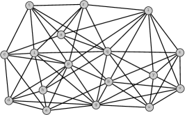
Figure 2: A candidate graph $B_{17}$ with $17$ vertices and $60$ edges

The exact number of optimal 1-planar graphs is known for graphs of size up to $36$. Bodendiek et al. [8] showed that $K_{6}$ is 1-planar but is not optimal and that there are no optimal 1-planar graphs with seven and nine vertices. There is a unique optimal 1-planar graph for $n=8,10,11$, and there are three optimal 1-planar graphs for $n=12,13$. For $n=14$, they found $11$ optimal 1-planar graphs, but one is missing. Brinkmann et al. [14] developed recurrence relations for the enumeration of quadrangulations and computed the number of 3-connected quadrangulations up to size $36$. For example, there are 12 for $n=14$ and 3000183106119 quadrangulations and optimal 1-planar graphs of size 36.

The pseudo-double wheels [14] and the extended wheel graphs $XW_{2k}$ play a particular role for quadrangulations and optimal 1-planar graphs, respectively, since thes are the irreducible or minimum graphs under two graph reduction rules. For $k\geq 3$, a pseudo-double wheel $W_{2k}$ is a quadrangulation with two distinguished vertices $p$ and $q$, called poles, a cycle of even length with vertices $v_{1},\ldots,v_{2k}$ and edges $(v_{i},v_{i+1})$ in circular order and further edges $(p,v_{2i})$ and $(q,v_{2i-1})$ for $i=1,\ldots,k$. Thus $p$ is connected with the vertices at even and $q$ with the vertices at odd positions on the cycle. $W_{2k}$ has $n=2k+2$ vertices, $2n-4$ edges and $n-2$ faces. The extended wheel graph $XW_{2k}$ additionally contains all possible pairs of 1-planar crossing edges $(p,v_{2i-1}),(v_{2i},v_{2i+2})$ and $(q,v_{2i}),(v_{2i-1},v_{2i+1})$ in circular order. This is the augmentation of $W_{2k}$ by kites, see Fig. 3. The two poles of $XW_{2k}$ have degree $2k$ and each of the $2k$ vertices on the cycle has degree six. If $k\geq 4$, then the edges $(v_{i},v_{i+1})$ on the cycle are black and the edges $(v_{2i},v_{2i+2})$ and $(v_{2i-1},v_{2i+1})$ are red. In addition, a graph is an extended wheel graph if it is optimal 1-planar and has a vertex of degree $n-2$ [8]. The second degree $n-2$ vertex is implied. Moreover, an optimal 1-planar graph is an extended wheel graph if the vertices of degree six form a cycle [8].

The notation $XW_{2k}$ for graphs of size $2k+2$ is taken from Suzuki [35] and is related to Schumacher’s $2*\hat{C}_{2k}$ notation.

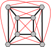
(a) The minimum extended wheel graph $XW_{6}$ drawn as a crossed cube

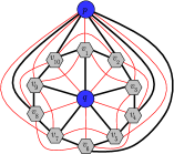
(b) The extended wheel graph $XW_{10}$ with poles $p$ and $q$ and with hexagons for vertices of degree $6$

Figure 3: Extended wheel graphs $XW_{6}$ and $XW_{10}$. Any two non-adjacent vertices $p$ and $q$ of $XW_{6}$ can be taken as poles. In larger extended wheel graphs, if poles $p$ and $q$ change places this swaps the coloring of the incident edges. Edges between consecutive vertices on the cycle are always planar and are colored black.

We summarize some basic properties of optimal 1-planar graphs from [7, 8, 35].

Proposition 1

Every optimal 1-planar graph $G=(V,E)$ consists of a planar quadrangulation $G_{P}=(V,E_{P})$ and a pair of crossing edges $e,f$ in each face of $G_{P}$ forming a kite such that $E=E_{P}\cup E_{C}$, where $E_{C}$ is the set of crossing edges. $G_{P}$ is 3-connected and bipartite. $G$ has a unique embedding, except if $G$ is an extended wheel graph $XW_{2k}$, which has two inequivalent embeddings for $k\geq 4$ in which the planar and crossing edges incident to a pole are interchanged and their colors swap. The minimum extended wheel graph $XW_{6}$ has six inequivalent 1-planar embeddings.

From the fact that $G_{P}$ is bipartite, we can conclude:

Lemma 1

Every cycle of odd length in an optimal 1-planar graph contains at least one red edge. If $C$ is a cycle of length four and three of its edges are black, then all edges of $C$ are black.

Schumacher [34] defined a relation on 1-planar embeddings and used it to characterize $5$-connected optimal 1-planar graphs.

Definition 1

Two 1-planar embeddings $\mathcal{E}(G)$ and $\mathcal{E}(G^{\prime})$ are related, $\mathcal{E}(G)\hookrightarrow\mathcal{E}(G^{\prime})$, if there is a planar quadrangle $(v_{1},v_{2},v_{3},v_{4})$ in the planar skeleton $P(\mathcal{E}(G))$ such that

(*)     all paths from $v_{1}$ to $v_{3}$ of length four in $P(\mathcal{E}(G))$ pass through $v_{2}$ or $v_{4}$.

Then $\mathcal{E}(G^{\prime})$ is obtained from $\mathcal{E}(G)$ by merging $v_{1}$ and $v_{3}$ and removing parallel edges. For graphs $G$ and $G^{\prime}$, let $G\hookrightarrow G^{\prime}$ if there exist embeddings such that $\mathcal{E}(G)\hookrightarrow\mathcal{E}(G^{\prime})$ and denote the transitive closure by “$\hookrightarrow^{*}$”.

The paths of (*) from $v_{1}$ to $v_{3}$ are simple and use only planar (black) edges. The embedding $\mathcal{E}(G)$ must satisfy special properties such that the planar quadrangle $(v_{1},v_{2},v_{3},v_{4})$ coincides with $(x,x_{3},x_{4},x_{5})$ in Fig. 5. Note that each quadrangle in an extended wheel graph has a path of length four between opposite vertices $(v_{i-1},v_{i+1})$ of a planar quadrangle through one of the poles, such that (*) is violated. In consequence, the “$\hookrightarrow$”-relation is not applicable.

Proposition 2

[34] Every 5-connected optimal 1-planar graph $G$ can be reduced to an extended wheel graph $XW_{2k}$ for some $k\geq 3$, i.e., $G\hookrightarrow^{*}XW_{2k}$. The extended wheel graphs are irreducible (or minimum) elements under the “$\hookrightarrow$”-relation.

By the restriction to 5-connected graphs, Schumacher excluded graphs with separating 4-cycles. Separating 4-cycles play a similar role in optimal 1-planar graphs as separating triangles do in triangulated planar graphs. In fact, every non-irreducible $5$-connected optimal 1-planar graph can be reduced to $XW_{8}$ [11].

Brinkmann et al. [14] introduced two graph transformations, called $P_{1}$-  and $P_{3}$-expansions, for the generation and characterization of (planar) 3-connected quadrangulations. We consider their inverse as reductions.

Definition 2

The $P_{1}$-reduction on a quadrangulation consists of a contraction of a face $f=(u,x,v,z)$ at $x,z$, where $x$ has degree $3$ and $u,v,z$ have degree at least $3$. It is shown in Fig. 4 and in an augmented version in Fig. 5 with the restriction to planar (black) edges. The $P_{3}$-reduction removes the vertices of the inner cycle of a planar cube, where the inner cycle is empty and the vertices of the outer cycle have degree at least $4$, see Fig. 6 restriced to planar (black) edges.

The reductions must be applied such that they preserve the class of 3-connected quadrangulations.

By the one-to-one correspondence between 3-connected quadrangulations and optimal 1-planar graphs, the $P_{1}$-  and $P_{3}$-reductions are extended straightforwardly to embedded 1-planar graphs, called vertex and face contraction by Suzuki [35]. Their inverse is called $Q_{v}$-splitting and $Q_{4}$-cycle addition, respectively, and are used from right to left. The illustration in Fig. 4 is taken from [35]. A $Q_{4}$-cycle addition removes the pair of crossing edges of a kite and inserts five new kites as illustrated in Fig. 6. Suzuki [35] observed that Schumacher’s “$\hookrightarrow$”-relation coincides with his face contraction and defines the $P_{1}$-reduction on the planar skeleton of an embedded 1-planar graph.

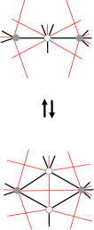
Figure 4: Face contraction or vertex splitting on 1-planar embeddings with planar (black and thick) and crossing (red and thin) edges

The distinction between graphs and embeddings is not important for the $P_{1}$-  and $P_{3}$-reductions of Brinkmann et. al., since there is a one-to-one correspondence on $3$-connected planar graphs. They point out that the reductions must be used with care such that the given class of graphs is preserved. It is not specified, however, how this is achieved. On the other hand, the “$\hookrightarrow$”-relation of Schumacher and the $Q_{v}$-splitting and $Q_{4}$-cycle addition and the inverse $Q_{f}$-contraction and $Q_{4}$-removal of Suzuki need a 1-planar embedding and the distinction between planar (black) and crossing (red) edges. It is not immediately clear how to apply these rules to graphs that are given without an embedding or an edge coloring. Nevertheless they characterize the respective graphs, as stated in Propositions 3 and 4.

3 Reduction Rules and Their Application

For the translation of the reduction rules from embeddings to graphs and an efficient check of their usability, we use the uniqueness of 1-planar embeddings of reducible optimal 1-planar graphs and the local environment of a reduction. In consequence, a reduction is applied to a subgraph which has (almost) a fixed embedding. A primary goal is to compute the embedding and to check the feasibility of the application of a reduction. The correctness follows from the works of Brinkmann et al. [14], Schumacher [34], and Suzuki [35].

Transformations on graphs and graph replacement systems have been studied in the theory of graph grammars [33]. In general, a graph transformation is a pair of left-hand and right-hand side graphs $\alpha=(L,R)$. An application of $\alpha$ to a graph $G$ replaces an occurrence of $L$ in $G$ by an occurrence of $R$ while the remainder $G-L$ is preserved. It results in a graph $G^{\prime}=G-L+R$. A graph $L$ occurs in $G$ and $L$ is said to match a subgraph $H$ of $G$ if there is a graph homomorphism between $L$ and $H$, which is one-to-one and onto on the vertices and one-to-one but not necessarily onto for the edges, and similarly for $R$ and $G^{\prime}$. Unmatched edges of $H$ remain in $G-L$ and are kept for $G-L+R$. This is elaborated in the algebraic approach to graph transformations [18]. In this particular case, the general approach does not really help, since the complexity of the element problem of graph grammars is PSPACE hard [9].

We reverse the expansions of Brinkmann et al. and Suzuki and call them SR-reduction (Schumacher reduction) and CR-reduction (crossed cube reduction), and the graphs of the left-hand sides $CS$ (crossed star) and $CC$ (crossed cube), respectively. The $SR$-reduction augments the vertex splitting of Suzuki and includes the subgraph induced by the center $x$. The reductions are shown in Figs. 5 and 6 including a 1-planar embedding and an edge coloring. The tiny strokes at the outer vertices indicate further edges, which are necessary. These vertices may have even more edges to outer vertices.

Following Brinkmann et al. [14], the given class, here the optimal 1-planar graphs, must be preserved and therefore an application of a reduction is constrained. An infeasible application may destroy the 3-connectivity of the underlying planar skeleton or introduce multiple edges, which ultimately leads to a violation of 3-connectivity.

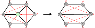
Figure 5: The reduction $SR(x\mapsto x_{4})$ for optimal 1-planar graphs. A candidate is drawn as a hexagon and other vertices as circles. Good candidates are light green and bad ones orange. Planar edges are drawn black and thick and crossing edges red and thin. The tiny strokes at the outside indicate further necessary edges. The left graph is $CS$ together with its embedding.

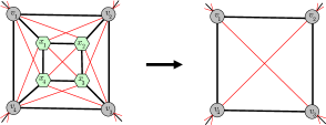
Figure 6: The reduction $CR(x_{1},x_{2},x_{3},x_{4})$ for optimal 1-planar graphs with candidates $x_{1},x_{2},x_{3},x_{4}$. The reduction is good and the candidates are colored light green if there is no edge $(v_{1},v_{3})$ or $(v_{2},v_{4})$ in the outer face. The graph on the left is $CC$ together with its embedding.

The main task of our algorithm is an efficient and feasible use of the reduction rules such that optimal 1-planar graphs are preserved. An obstacle is the gap between the graphs $CS$ and $CC$ of the left-hand side of the reductions, which come with an embedding, and the matched subgraph $H$, which comes as a part of $G$. A matched subgraph $H(x)$ of a $SR$-reduction is a subgraph induced by a vertex $x$ of degree six and its neighbors. There are three red and three black neighbors which alternate in the circular order around $x$. For a $CR$-reduction there is a subgraph of eight vertices. A matched subgraph may have further edges, since the matching is not onto for the edges. This introduces so-called blocking edges and is discussed later on. We grant 3-connectivity of the underlying planar skeleton by the absence of a blocking vertex, which has degree six. For example, vertices $x_{3}$ or $x_{5}$ are blocking vertices of $SR(x\mapsto x_{4})$ in Fig. 5 if they have degree six. In case of a $CR$-reduction, a vertex is blocking if it is matched by a vertex from the outer cycle of $CC$ and has degree six. Multiple edges are avoided by the absence of blocking edges, which can be planar or crossing, i.e., black or red. A blocking edge is always related to a reduction and it may be blocking for many reductions. Blocking black edges occur in separating 4-cycles, and red and black blocking edges are treated differently. Blocking vertices and planar blocking edges can also appear in the planar case, whereas blocking red edges are exclusive to 1-planar graphs. They also cover the case of blocking vertices, since a blocking vertex implies a blocking red edge. The converse does not hold.

A matching of $CS$ or $CC$ with a subgraph $H$ shall classify the edges of $H$ as planar and crossing and color them black and red, respectively. It shall determine the circular order of the vertices in the outer face of $CS$ and $CC$, and thus an embedding of $H$. However, this is not always the case. Graph $CS$ has several 1-planar embeddings, since some $K_{4}$’s may be drawn planar or as a kite. In fact, $CS$ is a planar graph, however, as a subgraph of a 1-planar graph it must be embedded with crossings as shown in Fig. 5, since reducible optimal 1-planar graphs have a unique embedding. Furthermore, if the matched graph of $CS$ also has edges $(x_{2},x_{6})$ and $(x_{3},x_{6})$, then it has two 1-planar embeddings in which $x_{1}$ and $x_{6}$ may change places, which implies a color change of the incident edges, just as in the case of extended wheel graphs. If edges $(x_{2},x_{4}),(x_{2},x_{6}$ and $(x_{4},x_{6})$ exists in addition to the edges of $CS$, then the situation is even worse and any circular order of the neighbors of $x$ is possible. Fortunately, these possibilities are represented by the degree vectors which are defined below.

The usability of a reduction is linked to one or four vertices of degree six and some conditions. A $SR$-reduction is applied to a vertex $x$ of degree six, which is the image of the central vertex and the corner of three kites of $CS$. For the right-hand side, $x$ is merged with a target, which is a red vertex $v$ of the outer cycle, denoted $SR(x\mapsto v)$, and $SR(x\mapsto x_{4})$ is shown in Fig. 5. A given optimal 1-planar graph may have several places for the application of a reduction, even at a single candidate, and the next reduction is chosen nondeterministically. There are candidates where a reduction is feasible and others where a reduction is infeasible. An application of a $CR$-reduction is linked to (one of) four vertices $x_{1},x_{2},x_{3},x_{4}$ of degree six, which are all infeasible for a $SR$-reduction, and is denoted $CR(x_{1},x_{2},x_{3},x_{4})$. The vertices are on the inner cycle of $CC$ and are removed and replaced by a pair of crossing edges, such that the vertices from the outer cycle form a kite. In a drawing, the inner cycle may be at the outside.

For convenience, we say that $SR$ is applied to vertex $x$ of the given graph if $SR(x\mapsto v)$ is feasible and call $v$ the target of $x$, and similarly, that $CR$ is applied to $(x_{1},x_{2},x_{3},x_{4})$ or just to $x_{i}$ for some $i=1,2,3,4$. In addition, we shall identify the vertices and edges of the left-hand sides $CS$ or $CC$ with those of the matched subgraph $H$, although the embedding and edge coloring of $H$ is not yet fixed and some vertices might change places. In general, the matching and embedding will be clear. Sometimes, it would be good to increase the degree of a vertex $u$, e.g., to avoid that $u$ is a blocking vertex for another reduction. The simplest way is to apply the inverse of $CR$, i.e., the $Q_{4}$-cycle addition of [35], and insert a new $4$-cycle together with five pairs of crossing edges in a quadrangular face at $u$ that is left if a pair of crossing edges is removed.

Definition 3

A vertex $x$ (of an optimal 1-planar graph $G$) of degree six is called a candidate.

A candidate $x$ is “good” if there is a feasible application of a reduction at $x$. Then the reduction is used as given in Figs. 5 and 6 and the class of optimal 1-planar graphs is preserved. A good candidate is drawn as a light green hexagon. In case of $SR$, $x$ is the center of a subgraph $H(x)$ of $G$ that matches $CS$ and there is some red neighbor $v$, called a target, such that $SR$ can be applied by merging $x$ with $v$, denoted $SR(x\mapsto v)$. Then $SR(x\mapsto v)$ is “good” and can feasibly be applied to $x$. There are three targets in $H(x)$ for a $SR$-reduction. In case of a $CR$-reduction, vertex $x$ belongs to the inner cycle of a subgraph $H$ that matches $CC$, and $CS$ is applied to any vertex of the inner cycle.

Otherwise, $x$ is a “bad” candidate and is drawn as an orange hexagon. Then the reductions $SR(x\mapsto v)$ are bad for all three red neighbors of $x$. The usage is illegal. A bad reduction $SR(x\mapsto v)$ is blocked by a vertex $u$ if $u$ is a black neighbor of $x$ and $v$ of degree six and if $u$ is any vertex on the outer cycle of degree six in case of $CR$, respectively. An edge $e=(u,v)$ of $H(x)$ is a blocking red edge of $SR(x\mapsto v)$ if $u$ is a red neighbors of $x$. Edge $e$ is a blocking black edge if $u$ is a black neighbor and $e$ is not matched by an edge of $CS$. If the outer cycle of $CC$ matches $(v_{1},v_{2},v_{3},v_{4})$, then edges $(v_{1},v_{3})$ and $(v_{2},v_{4})$ are blocking red edges of a $CR$-reduction.

A subgraph $H(x)$ with neighbors $(x_{1},\ldots,x_{6})$ of $x$ in circular order may have up to three blocking red edges, namely $(x_{2},x_{4}),(x_{4},x_{6})$ and $(x_{6},x_{2})$ if $x_{2},x_{4},x_{6}$ are the red neighbors of $x$, see Fig. 7. There may be none. Blocking red edges are associated in pairs with $SR$-reductions, and each blocking red edge $(u,v)$ is associated with two $SR$-reductions, $SR(x\mapsto u)$ and $SR(x\mapsto v)$. The edges must be red by Lemma 1. Accordingly, a blocking black edge $(u,v)$ of $SR(x\mapsto v)$ connects $v$ with the vertex at the opposite side of $CS$, since it is not matched, and, again, it must be black by Lemma 1, see Fig. 7. There are up to three blocking black edges in $H(x)$, and each $SR$-reduction has at most one blocking black edge, since blocking black edges do not cross. There are two blocking red edges in case a $CR$-reduction, however, at most one of them can occur in an optimal 1-planar graph that is not the minimum extended wheel graph $XW_{6}$. By Lemma 1, blocking black edges are excluded in this case.

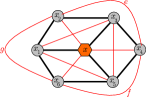
(a) Graph $CS$ with three blocking red edges $e,f$ and $g$. There may be a subgraph in the area between $e$ and (x2, x3, x4) and similarly for $f$ and $g$. $SR(x\mapsto x_{4})$ is blocked by $x_{3}$ if there is no such subgraph and $e$ is crossed by a red edge incident to $x_{3}$.

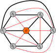
(b) Graph $CS$ with a blocking black edge and two blocking red edges

Figure 7: Blocking edges added to $CS$

An application of a reduction with a blocking vertex would decrease the degree of the blocking vertex to four, which would violate the 3-connectivity of the planar skeleton. The resulting graph would no longer be optimal 1-planar. The application of a reduction with a blocking edge would introduce a multiple edge, whose endpoints are a separation pair of the planar skeleton. This again leads to a violation of the 3-connectivity of the planar skeleton. Note that the case of a blocking vertex is covered by a blocking red edge between the black neighbors of the blocking vertex on the outer cycle. The converse is not true, since the blocking edge may enclose a (larger) subgraph. For example, add a forth vertex and then apply the inverse of $CR$.

Example 1

Consider graph $G_{17}$ which is optimal 1-planar by the 1-planar embedding displayed in Fig. 10(a). Vertices $a,c,d,h,r,s,t,u,v,y,z$ are candidates, where $a,c,h,s,t$ are good for a $SR$-reduction, whereas $d$ and $r$ are bad candidates, and therefore are colored orange. Vertices $u,v,y,z$ are good for a $CR$-reduction. A good $SR$-reduction $SR(x\mapsto v)$ is indicated by an arrowhead on the red edge from $x$ to $v$. Vertex $x$ moves along that edge and is merged with $v$. For example, $SR(a\mapsto b)$ is good, whereas $SR(a\mapsto c)$ and $SR(a\mapsto h)$ are bad, since $d$ is a blocking vertex and $(c,h)$ is a blocking red edge.

As another example, consider extended wheel graphs as in Fig. 3. Every vertex on the cycle of $XW_{2k}$ is a candidate which, however, is blocked by its neighbors on the cycle. In addition, all vertices of $XW_{6}$ are blocked candidates. Hence, all $SR$-reductions are bad and the extended wheel graphs are irreducible.

Definition 4

Every reduction $\alpha$ has a pair $\{e,f\}$ of associated red blocking edges. If $\alpha=SR(x\mapsto v)$, then $e=(u,v)$ and $f=(w,v)$, where $u,v$ and $w$ are the red neighbors of $x$. If $\alpha$ is a $CR$-reduction, then $e$ and $f$ are the two blocking red edges of $CC$.

Recall that $SR$ is Schumacher’s “$\hookrightarrow$”-relation and the reverse of Suzuki’s vertex splitting $Q_{v}$ [35], and $CR$ is the reverse of the $Q_{4}$-cycle addition, and the $P_{1}$-  and $P_{3}$-expansions of Brinkmann et al. are the restrictions to planar quadrangulations. The existential foundations for the reductions are:

Proposition 3

[14] The class $\mathcal{Q}_{3}$ of all 3-connected quadrangulations of the sphere is generated from the pseudo-double wheels by the $P_{1}(\mathcal{Q}_{3})$-  and $P_{3}(\mathcal{Q}_{3})$-expansions.

Proposition 4

[35] Every optimal 1-planar graph can be obtained from an extended wheel graph by a sequence of $Q_{v}$-splittings and $Q_{4}$-cycle additions.

3.1 Application of the Reduction Rules

For an application of a reduction one must find a matching of $CS$ and $CC$ and a subgraph $H$ that preserves the coloring and the 1-planar embedding of $CS$ and $CC$, respectively, and check whether the reduction is good or bad. In addition, the reason for a bad reduction must be known for the linear time algorithm in Section 4. Fortunately, the degree vector and the local degrees of the vertices of the matched subgraph provide the necessary information, as stated in Table 1.

Definition 5

Let $x$ be a candidate of graph $G$, and let $H(x)$ be the subgraph induced by $x$ and its six neighbors. Let $\overrightarrow{H(x)}=(d_{1},\ldots,d_{7})$ be the lexicographically ordered 7-tuple with the local degrees of the vertices of $H(x)$, called the degree vector of $x$, and call $\tau(x)=d_{1}$ the type of $x$.

Lemma 2

If $x$ is a candidate of an optimal 1-planar graph, then

1. $3\leq\tau(x)\leq 5$

2. $H(x)$ has between $15$ and $18$ edges, and

3. $\overrightarrow{H(x)}\in\{(3,3,3,5,5,5,6),(3,3,4,5,5,6,6),(3,4,4,5,5,5,6),(3,4,5,5,5,6,6)$,
              $(4,4,5,5,5,5,6),(4,4,5,5,6,6,6),(5,5,5,5,5,5,6)\}$.

Proof

The first tuple for $\overrightarrow{H(x)}$ is the degree vector of $CS$ and any sparser subgraph cannot match $CS$. As $x$ is the corner of three kites, one can add at most three extra edges in the outer face of $CS$, namely $(x_{2},x_{4}),(x_{2},x_{6}),(x_{6},x_{4})$ with $\overrightarrow{H(x)}=(5,5,5,5,5,5,6)$ and $(x_{2},x_{4}),(x_{2},x_{6}),(x_{2},x_{5})$ with $\overrightarrow{H(x)}=(4,4,5,5,6,6,6)$, where e.g., $(x_{2},x_{5})$ must be black and the other edges are red. The other degree vectors result from one or two edges added to $CS$. ∎

Obviously, $\overrightarrow{H(a)}=(3,4,4,5,5,5,6)$ for vertex $a$ of $G_{17}$ in Fig. 10(a) and vertex $b$ has local degree $3$. Moreover, $\overrightarrow{H(x)}=(4,4,5,5,5,5,6)$ if $x$ is on the inner cycle of $CC$ and the $CR$-reduction is good, such as $u,v,y,z$ in $G_{17}$, and if $x$ is on the cycle of an extended wheel graph $XW_{2k}$ for $k\geq 4$. Finally, the maximum degree vector $\overrightarrow{H(x)}=(5,5,5,5,5,5,6)$ appears at every vertex of $XW_{6}$ and at two candidates of $CC$ if there is a blocking red edge, e.g., $(b,g)$ in Fig. 11(b).

Definition 6

The subgraph $H(x)$ of a candidate $x$ of an optimal 1-planar graph is fixed if its embedding and coloring is uniquely determined. It has a partial coloring if two neighbors of $x$ may change places and the coloring of the incident edges is open, and, finally, $H(x)$ is unclear if the coloring of the edges of $H(x)$ is undecided.

Lemma 3

Let $x$ be a candidate of an optimal 1-planar graph $G$ and $H(x)$ the subgraph induced by $x$ and its neighbors.

1. If $\tau(x)=3$, then the coloring of $H(x)$ is fixed except for $\overrightarrow{H(x)}=(3,4,5,5,5,6,6)$, where there is a partial coloring.

2. If $\tau(x)=4$, then there is a partial coloring.

3. If $\tau(x)=5$, then the edge coloring is unclear.

Proof

First, a black neighbor of $x$ has local degree at least $5$.

If $\tau(x)=3$ and $x_{4}$ has local degree $3$, then $x_{4}$ is a red neighbor of $x$ and has two more neighbors, say $x_{3}$ and $x_{5}$, that are black neighbors of $x$ and $x_{4}$. Then the subgraph induced by $(x,x_{3},x_{4},x_{5})$ must form a kite, since it is $K_{4}$ and the embedding is unique by Proposition 1. If there is another vertex with local degree $3$, then the above applies again, such that the circular order of the neighbors of $x$, the edge coloring and the embedding of $H(x)$ are uniquely determined. If $d_{2}=d_{3}=4$, then the two vertices with local degree $4$ are red neighbors of $x$ and they have a red edge in between, whose removal leaves two vertices with local degree $3$. Again, $H(x)$ is uniquely determined. Finally, consider $\overrightarrow{H(x)}=(3,4,5,5,5,6,6)$ with $x_{4}$ of local degree $3$ and $x_{2}$ of local degree $4$. Vertex $x_{4}$ determines $x_{3}$ and $x_{5}$ as its black neighbors on the cycle. There are no edges $(x_{2},x_{4})$ and $(x_{2},x_{5})$ such that $x_{2}$ is opposite of $x_{5}$. Vertices $x_{2}$ and $x_{4}$ have $x_{3}$ as common neighbor and $x_{3}$ is a black neighbor of $x,x_{2}$ and $x_{4}$. However, the roles of $x_{1}$ and $x_{6}$ are undecided in $H(x)$. They may change places in the circular order around $x$, but the edge $(x_{1},x_{6})$ is black, see Fig. 8. Thus there is a partial coloring of $H(x)$.

If $\tau(x)=4$, there are two vertices of local degree $4$ by Lemma 2. Let $x_{2}$ and $x_{4}$ be these vertices, which are red neighbors of $x$. The third red neighbor of $x$ has local degree at least $5$. Hence, edge $(x_{2},x_{4})$ is missing in $H(x)$. There is a vertex of local degree $5$ that is not adjacent to $x_{4}$ and is opposite of $x_{4}$ and similarly for $x_{2}$. Let $x_{1}$ and $x_{5}$ be the respective vertices, which are black neighbors of $x$. Edges $(x_{1},x_{2})$ and $(x_{4},x_{5})$ are black, and the subgraph induced by $\{x,x_{1},x_{3},x_{4},x_{6}\}$ is fixed. However, $x_{3}$ and $x_{6}$ may change places and there is a partial edge coloring. Finally, the neighbors of $x$ are indistinguishable and the edge coloring is unclear if $\tau(x)=5$. ∎

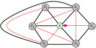
(a) The correct 1-planar drawing.

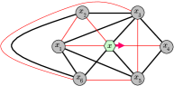
(b) The incorrect 1-planar drawing with a new edge coloring. For a correct drawing swap $x_{1}$ and $x_{6}$.

Figure 8: An ambiguous case where the embedding of $x_{1}$ and $x_{6}$ is not yet fixed.

Fortunately, neighboring candidates help each other in determining the edge coloring. Consider the candidates $x_{1},x_{2},x_{3},x_{4}$ of the inner cycle of $CC$, as given in Fig. 6, and assume that the graph is not $XW_{6}$. Then $\tau(x_{i})\geq 4$ and $\tau(x_{i})=4$ for two of them, say $x_{1}$ and $x_{3}$. Then $\overrightarrow{H(x_{1})}$ determines that $(x_{1},x_{2}),(x_{1},x_{4}),(x_{2},v_{2})$ and $(x_{4},v_{4})$ are black, whereas $v_{1}$ and $x_{3}$ may change places. Similarly, $\overrightarrow{H(x_{3})}$ determines the black edges $(x_{3},x_{2}),(x_{2},v_{2}),$ $(x_{3},x_{3}),$ $(x_{4},v_{4})$. If $\tau(x_{2})=5$ then $\tau(x_{4})=5$ and their coloring is unclear. However, the black neighbors of $x_{2}$ are $x_{1},v_{2},x_{3}$ and $v_{1}$ is a red neighbor, which implies that $v_{1}$ is a black neighbor of $x_{1}$ and the case is decided. Hence, the coloring of a subgraph matching $CC$ is fixed and its embedding is unique.

In fact, we have the following situation:

Lemma 4

Let $H$ be a (sub-) graph of size $7$ with a vertex $x$ of degree $6$. Then $H$ is unique and is maximal planar if $\overrightarrow{H(x)}=(3,3,3,5,5,5,6)$. There are (at least) two graphs $H_{1}$ and $H_{2}$ if $\overrightarrow{H(x)}=(3,4,4,5,5,5,6)$, and $H_{1}$ and $H_{2}$ are non-planar and $1$-planar.

Proof

Let $\{x,v_{1},\ldots,v_{6}\}$ be the vertices of $H$, where $x$ has degree $6$, and $v_{2},v_{4},v_{6}$ have local degree $3$. If each of $v_{2},v_{4},v_{6}$ has two vertices of $v_{1},v_{3},v_{5}$ as neighbors, then $H=CS$. Clearly, $CS$ satisfies the assumptions and is planar. For a contradiction, suppose that there is an edge $(v_{2},v_{4})$ and let $u,v$ be the two remaining neighbors of $v_{2}$ and $v_{4}$. Then $v_{1},v_{3}$ and $v_{5}$ cannot have local degree $5$ and there is no graph as required.

Let $H_{1}$ be obtained from $CS$ by adding edge $(x_{2},x_{4})$, and let $H_{2}$ be the graph displayed in Fig. 9. There is an edge from the vertex of degree $3$ to a vertex of degree $4$ in $H_{2}$, which does not exist in $H_{1}$. The graphs are non-planar, since there are $7$ vertices and $16$ edges and they are 1-planar, as shown by the figures. ∎

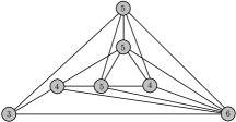
Figure 9: Graph $H_{2}$ from Lemma 4 with vertices labeled by degree

Similarly, there is a unique subgraph that matches $CC$ if $CR$ is good. The unique embedding is obtained from pairs of vertices that are placed opposite each other on the inner and outer cycles.

Lemma 5

There is a unique graph $H$ that matches $CC$ if $H$ has four mutually neighbored candidates $x_{1},x_{2},x_{3},x_{4}$ with $\overrightarrow{H(x_{i})}=(4,4,5,5,5,5,6)$ for $i=1,2,3,4$.

Proof

Let $v_{1},v_{2},v_{3},v_{4}$ be the remaining vertices of $H$. Each vertex of the inner cycle of $CC$ excludes exactly one vertex of the outer cycle as a neighbor. Assume this does not hold in $H$ and let e.g., $x_{1}$ and $x_{2}$ both exclude $v_{1}$ as a neighbor. Since $x_{1}$ and $x_{2}$ are candidates, vertices $v_{2},v_{3},v_{4}$ are their neighbors, and both $x_{1}$ and $x_{2}$ contribute a $6$ in the degree vector of the other such that $\overrightarrow{H(x_{1})}=(\ldots,6,6)$, a contradiction. ∎

The usability of a reduction is completely determined by the degree vector of a candidate and the type distinguishes between a $SR$-  and a $CR$-reduction.

Lemma 6

A candidate $x$ of an optimal 1-planar graph is good for $SR$ if and only if $\tau(x)=3$ and $SR(x\mapsto v)$ is good if $v$ has local degree $3$.

Proof

Let $H(x)$ be the subgraph matching $CR$ and let $\{x,x_{1},\ldots,x_{6}\}$ be the vertices of $H(x)$. Then $H(x)$ has a unique embedding matching the embedding of $CS$ as shown in Lemma 3 if $\tau(x)=3$ and $\overrightarrow{H(x)}\neq(3,4,5,5,5,6,6)$. Then $SR(x\mapsto x_{4})$ is good if $x_{4}$ has local degree $3$. Otherwise, there is a partial coloring and $x_{1}$ and $x_{6}$ may change places if $x_{4}$ has local degree $3$ and $x_{2}$ has local degree $4$. This ambiguity does not hinder using $SR(x\mapsto x_{4})$, which removes $x$ and the edge $(x_{3},x_{5})$ and inserts the edges $(x_{1},x_{4}),(x_{6},x_{4})$ and the red edge $(x_{2},x_{4})$. Then the color of the edges incident to $x_{1}$ and $x_{6}$ remains open.

If $\tau(x)\geq 4$, then every red neighbor of $x$ has a blocking red edge and there is no good $SR$-reduction. ∎

Lemma 7

A candidate $x_{1}$ of an optimal 1-planar graph is good for $CR$ if and only if $\tau(x_{1})=4$ and there are three more candidates $x_{2},x_{3},x_{4}$ with $\overrightarrow{H(x_{i})}=(4,4,5,5,5,5,6)$, and $CC$ matches the subgraph induced by $x_{1},x_{2},x_{3},x_{4}$ and its four common neighbors.

Proof

If $CR$ is good, then the degree vector of the four vertices that match the vertices of the inner cycle of $CC$ is $(4,4,5,5,5,5,6)$. The degree vector $(5,5,5,5,5,6,6)$ implies a blocking red edge and $\overrightarrow{H(x)}=(4,4,5,5,6,6,6)$ implies a black edge between two opposite neighbors of a center, which violates $CC$.

Conversely, there is a unique subgraph matching $CC$ by Lemma 5 if the degree vector of the candidates is $\overrightarrow{H(x)}=(4,4,5,5,6,6,6)$, and there is no blocking edge. ∎

Corollary 1

For each candidate $x$ of a graph $G$ it can be checked in $O(1)$ time whether $x$ is good or bad. It can be determined which reduction applies if $x$ is good. The reduction takes $O(1)$ time including a (partial) coloring of the edges.

Proof

The type of $x$ decides which reduction may apply and the degree vector(s) and the local degrees tell whether the reduction is good. The reductions operate on subgraphs with six resp. eight vertices. They remove one or four vertices and one more edge and insert three or two edges. This can be accomplished in $O(1)$ time. ∎

We summarize the degree vectors and their impact on an edge coloring, reductions and their blocking edges, and storing the reductions in the linear-time algorithm in Section 4 in Table 1. For convenience, assume that the circular order of the neighbors of candidate $x$ is $(x_{1},\ldots x_{6})$ as in Fig. 5, where $x_{2},x_{4}$ and $x_{6}$ are red neighbors and $x_{4}\leq x_{2}\leq x_{6}$ if the vertices are ordered by local degree. Let $e=(x_{2},x_{4}),f=(x_{6},x_{4}),g=(x_{2},x_{6})$ and let $d$ and $d^{\prime}$ be the diagonals $(v_{1},v_{3})$ and $(v_{2},v_{4})$ in case of $CC$ and a $CR$-reduction.

$\overrightarrow{H(x)}$	coloring	reductions	blocking edges	storing
$(3,3,3,5,5,5,6)$	fixed	$SR(x\mapsto x_{2})$	none	$GOOD_{e},GOOD_{g}$
		$SR(x\mapsto x_{4})$	none	$GOOD_{e},GOOD_{f}$
		$SR(x\mapsto x_{6})$	none	$GOOD_{f},GOOD_{g}$
$(3,3,4,5,5,6,6)$	fixed	$SR(x\mapsto x_{2})$	none	$GOOD_{e},GOOD_{g}$
		$SR(x\mapsto x_{4})$	none	$GOOD_{e},GOOD_{f}$
		$SR(x\mapsto x_{6})$	black	none
$(3,4,4,5,5,5,6)$	fixed	$SR(x\mapsto x_{2})$	$g$	$WAIT_{e},BAD_{g}$
		$SR(x\mapsto x_{4})$	none	$GOOD_{e},GOOD_{f}$
		$SR(x\mapsto x_{6})$	$g$	$WAIT_{f},BAD_{g}$
$(3,4,5,5,5,6,6)$	partial	$SR(x\mapsto x_{2})$	$g$	$WAIT_{e},BAD_{g}$
		$SR(x\mapsto x_{4})$	none	$GOOD_{e},GOOD_{f}$
		$SR(x\mapsto x_{6})$	black	none
$(4,4,5,5,5,5,6)$	fixed	$CR$	none	$GOOD_{d},GOOD_{d^{\prime}}$
$(4,4,5,5,6,6,6)$	fixed	$CR$	$d$	$BAD_{d},WAIT_{d^{\prime}}$
$(5,5,5,5,5,5,6)$	unclear	infeasible

Table 1: Degree vectors and their impact on reductions

The existence of a good candidate is granted unless all candidates are blocked, as in an extended wheel graph, or if the graph is not optimal 1-planar.

Lemma 8

If $G$ is a reducible optimal 1-planar graph, then $G$ has a good candidate.

Proof

According to Brinkmann et al. [14] there is a good candidate for their $P_{1}$-  and $P_{3}$-reductions (or expansions) on 3-connected quadrangulations unless the graph is a double-wheel graph, and thus irreducible. In Lemma 4 [14] they prove that a good candidate lies in the innermost (or outermost) separating $4$-cycle. By the one-to-one correspondence between planar 3-connected quadrangulations and optimal 1-planar graphs, this generalizes to optimal 1-planar graphs. ∎

As a final step, we consider the recognition of extended wheel graphs.

Lemma 9

There is a linear time algorithm to test whether a graph is an extended wheel graph $XW_{2k}$.

Proof

If the input graph $G$ has eight vertices, we check $G=XW_{6}$ by inspection. Here, each vertex $x$ is a candidate with $\overrightarrow{H(x)}=(5,5,5,5,5,5,6)$.

For $k\geq 4$, an extended wheel graph $XW_{2k}$ has two poles $p$ and $q$ of degree $2k$ as distinguished vertices and a cycle of $2k$ vertices of degree six. This is checked in a preprocessing step on the given graph and takes en passant $O(1)$ time. For a final check, we remove the poles and restrict ourselves to the subgraph induced by the vertices of degree six. Each such vertex $v$ has four neighbors and the cyclic ordering of these vertices is determined as $(v_{-2},v_{-1},v,v_{+1},v_{+2})$ by the missing edges $(v_{-2},v_{+1}),(v_{-2},v_{+2})$ and $(v_{-1},v_{+2})$. So we determine the cycle and then check for $XW_{2k}$. Altogether, the tests take $O(2k)$ time. ∎

From the above observations, we obtain a simple quadratic-time algorithm for the recognition of optimal 1-planar graphs. The algorithm scans the actual graph and searches a single candidate for $SR$ or a cluster of four candidates for $CR$ and checks in $O(1)$ time whether the reduction is good or bad. Each reduction removes one or four vertices. Hence, there are at most $n-2k-2$ reductions from a graph of size $n$ to an extended wheel graph $XW_{2k}$.

Theorem 3.1

There is a quadratic-time recognition algorithm for optimal 1-planar graphs.

Example 2

For an explanation of the reductions consider the input graph $G_{17}$ as shown in Fig. 10(a) with a 1-planar embedding. Vertices $a,c,h,s,t$ are good for an $SR$-reduction, and $u,v,y,z$ are good for a $CR$-reduction. If the $CR$-reduction is applied first, we obtain the graph in Fig. 10(b) and $SR(h\mapsto q)$ then yields $XW_{10}$.

Alternatively, using $SR(a\mapsto b),SR(h\mapsto q),SR(g\mapsto d),SR(c\mapsto b),SR(d\mapsto i)$ and finally $CR(u,v,y,z)$ ends up at $XW_{6}$. This computation is illustrated in Figs. 11(a) to 11(f). Note that the cluster $u,v,y,z$ flips from good to bad if there is an outer neighbor of degree six, which is blocking and induces a blocking red edge.

Also, $XW_{8}$ can be obtained by $SR(a\mapsto b),SR(h\mapsto q),SR(g\mapsto d)$, and finally $CR(u,v,y,z)$.

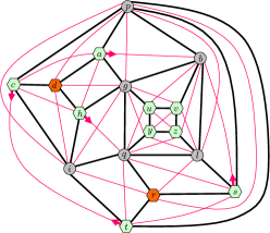
(a) A 1-planar embedding of $G_{17}$. Candidates are drawn as hexagons which are light green for good candidates and orange for bad candidates. Non-candidates of degree at least $8$ are drawn as circles.

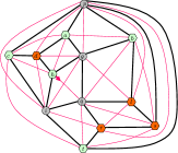
(b) Graph $G_{17}$ after $CR(u,v,y,z)$.

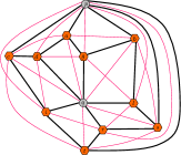
(c) and $XW_{10}$ after $SR(h\mapsto q)$.

Figure 10: A reduction of an input graph to an extended wheel graph.

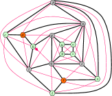
(a) after $SR(a\mapsto b)$

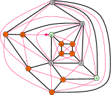
(b) and after $SR(h\mapsto q)$

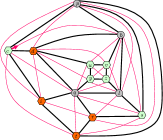
(c) and after $SR(g\mapsto d)$

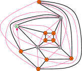
(d) and after $SR(c\mapsto b)$

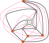
(e) and after $SR(d\mapsto i)$

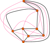
(f) and finally $CR(u,v,y,z)$ yields $XW_{6}$

Figure 11: A alternative reduction of an input graph to $XW_{6}$.

Graph $G_{17}$ in Example 2 can be reduced to different extended wheel graphs which are irreducible. In consequence, the graph reduction system with the rules $SR$ and $CR$ cannot be confluent, since confluence implies a unique irreducible representative. A rewriting system is confluent if $x\rightarrow^{*}u$ and $x\rightarrow^{*}v$ implies that there is a common descendant $z$ with $u\rightarrow^{*}z$ and $y\rightarrow^{*}z$. In consequence, if two rules can be applied at different places of $x$ starting two reductions, then the reductions join at a common descendant. This is not the case for $SR$ and $CR$. More properties are elaborated in [11].

Corollary 2

The reduction system with the rules $SR$ and $CR$ is non-confluent on optimal 1-planar graphs.

4 A Linear Time Algorithm

Example 2 shows that a reduction may change the role of other candidates and reductions. In particular, $SR(x\mapsto x_{4})$ increases the degree of $x_{4}$ by two. If $x_{4}$ was a candidate before, it is no longer. If $x_{4}$ blocked another reduction, it does no longer. On the other hand, the degree of $x_{3}$ and $x_{5}$ decreases by two and they may become new candidates, which may turn their neighbor candidates from good to bad. Accordingly, a $CR$-reduction decreases the degree of the vertices on the outer cycle by two, which may introduce some of them as candidates with an impact on candidates in their neighborhood. However, vertices at distance at least three from the vertex of the application of a rule are not affected. Hence, a reduction operates locally. However, a reduction may have a global effect and introduce or remove a blocking edge for many other reductions and candidates. This is illustrated in Figs. 12 and 13. Thus it may be advantageous to maintain lists with all reductions that are or may be blocked by an edge. There is a separating $4$-cycle if an edge blocks two or more reductions. Clearly, there is a separating $4$-cycle at a $CR$-reduction. If two $SR$-reductions are blocked by an edge $e=(u,v)$, then the centers of the reductions have degree $6$ and have $u$ and $v$ as common neighbors and there is a separating $4$-cycle through $u$ and $v$ which includes $e$ if the blocking edge is black.

We shall assume throughout that the given graph $G$ is reducible, i.e., not an extended wheel graph, and that $x$ is a candidate of a $SR$-reduction or $x$ is one of four candidates of a $CR$-reduction.

The degree vector of a candidate $x$ does not determine the coloring of $H(x)$, but it tells which reduction is applicable, see Lemmas 3 - 7. Infeasible applications can be restricted even further.

First, observe that $\tau(x)\leq 4$ if $x$ is a candidate of a reducible optimal 1-planar graph. Otherwise, $\overrightarrow{H(x)}=(5,5,5,5,5,5,6)$ implies $H(x)=K_{6}$, but $K_{6}$ is not a proper subgraph of a $5$-connected 1-planar graph [8].

Second, both blocking edges of a $CR$-reduction cannot occur simultaneously, since the induced subgraph would have a separation pair violating $4$-connectivity.

Finally, suppose there is a blocking black edge for an $SR$-reduction at candidate $x$, say edge $(x_{3},x_{6})$. Then $\overrightarrow{H(x)}=(3,3,4,5,5,6,6)$ or $\overrightarrow{H(x)}=(3,4,5,5,5,6,6)$ by Lemma 2. If vertex $x_{4}$ has local degree three, then $SR(x\mapsto x_{4})$ is applicable, whereas $SR(x\mapsto x_{6})$ is not. Suppose the coloring is fixed as in Fig. 5, otherwise one must also consider cases with $x_{1}$ and $x_{6}$ exchanged. Then $(x_{1},x_{2},x_{3},x_{6})$ and $(x_{1},x_{6},x_{4},x_{3})$ are separating $4$-cycles which separates $x$ from further black neighbors of $x_{2}$ and $x_{4}$, respectively. The blocking black edge $(x_{3},x_{6})$ for $SR(x\mapsto x_{6})$ cannot be removed if $x$ remains as a candidate. Then another reduction must remove the edge. A black edge is removed by a reduction if it is incident to a candidate. However, if $x$ is a candidate and there is the edge $(x_{3},x_{6})$, then $x_{3}$ has degree at least eight and the degree of $x_{3}$ cannot be decreased to six since $x$ is a blocking neighbor. Consider the $4$-cycle $C=(x_{1},x_{2},x_{3},x_{6})$ and suppose that $x$ is in the outer face of $C$, the other case is similar. Then $x_{2}$ has at least one more black neighbor $w$ besides $x_{1}$ and $x_{3}$. If $x_{6}$ had local degree six, then the red edge $(x_{6},w)$ were crossed by $(x_{1},x_{3})$, which were a multiple edge. Hence, also $x_{6}$ has degree at least eight and is not a candidate. Hence, the black prohibited edge $(x_{3},x_{6})$ remains if $x$ remains. However, if $SR(x\mapsto x_{2})$ or $SR(x\mapsto x_{4})$ can be applied, then $x$ is removed and also $SR(x\mapsto x_{6})$. In consequence, a reduction $SR(x\mapsto v)$ can never be used if there is a blocking black edge incident to $v$, and we add “none” in the last column of Table 1.

We summarize these facts:

Lemma 10

For a reducible optimal 1-planar graph the following holds:

1. If $x$ is a candidate, then $H(x)$ is fixed or has a partial coloring for an $SR$-reduction.

2. The subgraph matched by $CC$ has at most one blocking red edge.

3. A reduction $SR(x\mapsto v)$ is infeasible if there is a blocking black edge incident to $v$.

Next, consider the interaction between $SR$- and $CR$-reductions. Their usability is distinguished by the type of the candidates. The vertices of the inner cycle of $CC$ mutually block each other for a $SR$-reduction. These vertices are a “black hole” for $SR$-reductions, since they can never take the role of the center of a good $SR$-reduction. However, vertex $x$ of the inner cycle of $CC$ may be the target of a $SR$-reduction $SR(w\mapsto x)$, whose use absorbs vertex $w$. In that case, the $CR$-reduction is bad and is blocked by $w$. The vertices of the inner cycle can only be removed by a $CR$-reduction, or they remain for the final extended wheel graph.

Lemma 11

A $SR$-reduction never applies to a candidate $x_{i}$ if a $CR$-reduction applies to candidates $x_{1},x_{2},x_{3},x_{4}$ for $i=1,2,3,4$.

Proof

If $CR$ applies to $x_{1},x_{2},x_{3},x_{4}$, then $\overrightarrow{H(x_{i})}=(4,4,5,5,5,5,6)$ for $i=1,2,3,4$ if the reduction is good and $\overrightarrow{H(x_{i})}=(5,5,5,5,5,5,6)$ for two vertices if the reduction is bad by Lemma 7. The matching subgraph has a unique embedding. Vertices $x_{i}$ on the inner cycle of $CC$ mutually block each other and $\tau(x_{i})\geq 4$ excludes the use of a $SR$-reduction, which needs $\tau(x_{i})=3$ by Lemma 6. ∎

Finally, consider the relationship between reductions and blocking edges. A reduction may introduce a blocking edge for many reductions, and it may be blocked by several blocking edges. It is a many-to-many relation, say $(j:k)$, where $k$ may be linear in the size of the graph. By Lemma 10 it suffices to consider reductions with a fixed or a partial coloring, and a reduction with a blocking black edge can be discarded. Hence, a candidate $x$ may allow for three $SR$-reductions towards its red neighbors if $H(x)$ is fixed. Each $SR$-reduction has zero, one, or two blocking red edges, where zero means that the reduction is good. Therefore, $j\leq 2$ suffices. There are two bad $SR$-reductions for a candidate $x$ if there is a single blocking red edge, and $x$ is bad if and only if there are two blocking red edges or the graph is $XW_{6}$.

A $SR$-reduction $SR(x\mapsto x_{4})$ introduces the planar edge $(x_{1},x_{4})$, which simultaneously may close many 4-cycles and then may block many other candidates and their $SR$-reduction towards $x_{4}$, see Fig. 12. Similarly, edges $(x_{2},x_{4})$ and $(x_{6},x_{4})$ or the diagonals in $CR$ may be blocking red edges for many other reductions, as Fig. 13 illustrates. Such edges may be removed by another reduction, and then they can reappear after a further reduction.

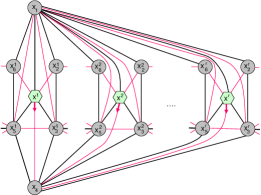
Figure 12: A conflict among good candidates $x^{1},\ldots,x^{r}$ and their $SR$-reduction $SR(x^{i}\mapsto x_{4})$. The first such reduction generates a blocking black edge and blocks the other reductions.

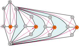
Figure 13: Illustration of a blocking red edge $(x_{2},x_{4})$ with many conflicts. There must be subgraphs in the shaded areas. If edge $e=(x_{2},x_{4})$ is introduced, e.g., by $SR(x\mapsto v_{4})$, then $e$ blocks the reductions $SR(x^{i}\mapsto x_{4})$ for $i=1,\ldots,r$. If $e$ is removed thereafter, it can be reintroduced by $SR(x^{j}\mapsto x_{4})$ for some $j$ and then it blocks the remaining $SR$-reductions again.

A direct treatment of all candidates and their reductions may lead to a quadratic running time. We use lists for the reductions that a red edge may block. For example, all reductions $SR(x^{i}\mapsto x_{4})$ and $SR(x\mapsto x_{4})$ in Fig. 13 are collected in a list $BAD_{e}$ if edge $e=(x_{2},x_{4})$ exists. The existence of a blocking red edge associated with a $SR$-reduction is determined by the degree vector and the local degree of the vertices. The outcome is given in Table 1 and is a consequence of Lemmas 6, 7 and 10.

To manage the reductions efficiently, we split each pair of associated blocking red edges of a reduction and treat each edge separately. For each red edge that occurs in $H(x)$ for some candidate $x$, there are three lists of reductions $GOOD_{e},BAD_{e}$ and $WAIT_{e}$ and two entries of each reduction as given in Table 1. Hence, there are up to six entries of $SR$-reductions at a candidate. A reduction $\alpha$ is good if and only if $\alpha$ is not blocked by an edge if and only if $\alpha$ is stored in $GOOD_{e}$ and in $GOOD_{f}$ or $WAIT_{f}$ and $\alpha$ is not blocked by a black edge. Here $e$ and $f$ are the blocking red edges associated with $\alpha$. If $\alpha$ is blocked by $f$ and is not blocked by $e$, then $\alpha$ is stored in $WAIT_{e}$ and in $BAD_{f}$ and, finally, $\alpha$ is stored in $BAD_{e}$ and in $BAD_{f}$ if both associated edges are blocking. In consequence, $BAD_{e}$ is empty if edge $e$ does not exist and, conversely, $GOOD_{e}$ and $WAIT_{e}$ are empty if $e$ exists.

However, it may happen that reduction $\alpha$ appears in $GOOD_{e}$ although $\alpha$ is blocked by the other blocking red edge $f$, and, conversely, that $\alpha$ appears in $WAIT_{e}$ although $\alpha$ is good. This happens unnoticed to $e$ and $GOOD_{e}$ if edge $f$ is (re)introduced or is removed, as indicated in Fig. 13. If $\alpha$ is accessed via $GOOD_{e}$ and $\alpha$ is bad, then there is an unsuccessful access, and $\alpha$ is moved from $GOOD_{e}$ to $WAIT_{e}$.

$CR$-reductions have a higher priority than $SR$-reductions. If it is encountered that a candidate $x$ has become a vertex of the inner cycle of $CC$, then its $SR$-reductions are removed from the lists and are replaced by the $CR$-reduction. This situation is detected as described in Lemma 7 and is justified by Lemma 11. In other words, $CR$ overrules $SR$.

In the next step of a computation a $\alpha$ is accessed via $GOOD_{e}$ for some edge $e$. Then it is checked whether $\alpha$ is good and if so, $\alpha$ is applied and some further actions are taken. Otherwise, there is an unsuccessful access. Then $\alpha$ is moved from $GOOD_{e}$ to $WAIT_{e}$ if there is the other blocking red edge $f$, and $\alpha$ is removed from the lists if $\alpha=SR(x\mapsto v)$ and there is a blocking black edge incident to $v$.

Suppose a reduction $SR(x\mapsto x_{4})$ is good and is applied as shown in Figs. 5 or 14. The case of a $CR$-reduction is similar, and even simpler. The actual graph is modified as described by the $SR$-reduction. Vertex $x$ is removed and so are all reductions at $x$ that are stored in the lists $GOOD_{e},BAD_{e}$, and $WAIT_{e}$. Also all lists with a red edge $e=(x,y)$ for some $y$ are removed. There are three vertices $y$, since $x$ is a candidate, and these removals take constant time. If $x_{4}$ was a candidate before, all reductions at $x_{4}$ are removed, since $x_{4}$ is no longer a candidate.

The $SR$-reduction removes edge $e=(x_{3},x_{5})$. Therefore, $BAD_{e}$ is renamed to $GOOD_{e}$. This makes the stored reductions accessible in the next step. Conversely, $GOOD_{e}$ and $WAIT_{e}$ are renamed to $BAD_{e}$ for $e=(x_{2},x_{4})$ and $e=(x_{6},x_{4})$, since these edges are introduced and may be blocking red edges for other reductions. Edge $h=(x_{1},x_{4})$ may become a blocking black edge, see Fig. 12. Here, no action is taken and reductions blocked by $h$ are removed at an unsuccessful access or if one of $x_{1}$ or $x_{4}$ is removed. Finally, vertices $x_{3}$ and $x_{5}$ may change their status and become a candidate. We consider $x_{3}$; the case of $x_{5}$ is similar. If vertex $x_{3}$ has become a candidate, then the possible reductions on $x_{3}$ are computed and are added to the respective lists $GOOD_{e},BAD_{e},WAIT_{e}$ and $GOOD_{f},BAD_{f},WAIT_{f}$ for the pair of associated red edges $e$ and $f$. Here $CR$ may overrule $SR$.

A change of the status of $x_{4}$ to a non-candidate and of $x_{3}$ and $x_{5}$ to a candidate has side effects on their neighbors if they were candidates, too. This is illustrated by the color change of candidates in Figs. 11(a) to 11(f) and in Fig. 14. However, there is no need for a special treatment, since everything is done by renaming the lists.

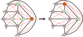
Figure 14: An update by $SR(x\mapsto x_{4})$ with candidates in the neighborhood.

Our linear time algorithm operates in three phases. First, it makes a static check that all vertices of the input graph $G$ of size $n$ have even degree at least six and that there are $4n-8$ edges. Then it sweeps the given graph for candidates $x$, checks $H(x)$, classifies and stores the reductions, and colors as many edges as possible. A second sweep may be helpful to clear some partial colorings. In general, it creates six entries for the $SR$-reductions at a candidate $x$ and stores them in the lists $GOOD_{e},BAD_{e}$, and $WAIT_{e}$ for each associated blocking red edge $e$. Two entries are discarded if there is a blocking black edge. If there is a $CR$-reduction at $x$, then two entries are created and $SR$-reductions at $x$ are removed immediately. If, surprisingly, the coloring of $G$ is complete, we are done. The planar skeleton is 3-connected and has a unique embedding and we test straightforwardly whether $G$ is optima1 1-planar. In general, there is a computation by a sequence of steps and each step is a reduction on a presumably optimal 1-planar graph $G=G_{0}\rightarrow G_{1}\rightarrow\ldots\rightarrow G_{t}=XW_{2k}$ for some $k\geq 3$ and $t\geq 0$. The algorithm immediately stops and reports a failure if the conditions for the application of a reduction are not met or there is a mismatch in the edge coloring between the graph and a reduction.

The algorithm has access to the lists $GOOD_{e}$, which, internally, are combined to a superlist. The data structure resembles an adjacency list for storing graphs. Empty sublists are removed. The algorithm renames lists which, internally, means removing and inserting sublists and takes $O(1)$ time. There is no preference or restriction for the manipulation of the superlist, which can be organized as a stack or as a queue or at random. The next reduction is taken from the neighborhood of the previous one if the superlist is organized as a stack, and all candidates of a given graph are checked sequentially if there is a queue. Moreover, one may use $CR$-reductions with higher priority than $SR$-reductions, since they remove four vertices in a step and have only two entries. Anyhow, there is a linear running time.

Input: A graph $G$

Output: $G$ is optimal 1-planar or fail

Data: A collection of lists $GOOD_{e}$, $BAD_{e}$ and $WAIT_{e}$ for some edges $e$. Each list contains reductions $\alpha=SR(x\mapsto x_{4})$ or $\alpha=CR(u,v,y,z)$ with candidates $x,u,v,y,z$.

1 // Preprocessing

2 if $\neg$($G$ has $4n-8$ edges and all vertices have even degree $\geq 6$) then return fail

3 // Initialization

4 foreach candidate $x$ of $G$ do call ADD_REDUCTIONS

5

6// Processing

7 while there is a reduction $\alpha$ accessible via $GOOD_{e}$ for some edge $e$ do

8      if $\alpha$ is good then

9             apply $\alpha$ and update $G$ and the coloring

10             remove all reductions at vertex $x$ from the lists $GOOD_{e},BAD_{e}$ and $WAIT_{e}$

11             if $\alpha=SR(x\mapsto x_{4})$ then

12                  remove all reductions on $x_{4}$ from the lists $GOOD_{e},BAD_{e}$ and $WAIT_{e}$

13                   remove all lists with $e=(x,y)$

14                   if $x_{3}$ is a candidate after the $SR$-reduction then call ADD_REDUCTIONS

15                   if $x_{5}$ is a candidate after the $SR$-reduction then call ADD_REDUCTIONS

16                   for $e=(x_{3},x_{5})$ do rename $BAD_{e}$ to $GOOD_{e}$

17                   for $e=(x_{2},x_{4})$ and $e=(x_{6},x_{4})$ do rename $GOOD_{e}$ and $WAIT_{e}$ to $BAD_{e}$

18                  

19             else  // $\alpha$ is a $CR$-reduction with outer cycle $(v_{1},v_{2},v_{3},v_{4})$

20                  apply $\alpha$ and update $G$ and the coloring

21                   for $v=v_{1},v_{2},v_{3},v_{4}$ do

22                        if $v$ is a candidate then call ADD_REDUCTIONS

23                        

24                   for $e=(v_{1},v_{3})$ and $e=(v_{2},v_{4})$ do rename $GOOD_{e}$ and $WAIT_{e}$ to $BAD_{e}$

25                  

26            

27       else  // an unsuccessful access to a reduction

28            if $\alpha=SR(x\mapsto v)$ has a blocking black edge incident to $v$ then remove $\alpha$ from the lists

29             else move $\alpha$ from $GOOD_{e}$ to $WAIT_{e}$

30            

31      

32 if $G$ is an extended wheel graph then return $G$ is optimal 1-planar

33 else return fail

Algorithm 1 OPTIMAL 1-PLANARITY TESTING

Input: A candidate $x$ and lists $GOOD_{e}$, $BAD_{e}$ and $WAIT_{e}$ for some edges $e$

Output: lists $GOOD_{e}$, $BAD_{e}$ and $WAIT_{e}$

1 if $x$ belongs to the inner cycle of $CC$ with outer cycle $(v_{1},v_{2},v_{3},v_{3})$ then

2       for $e=(v_{1},v_{3})$ and $f=(v_{2},v_{4})$ do

3            if $e$ exists then add $CR(x)$ to $BAD_{e}$ and to $WAIT_{f}$

4             else if $f$ exists then add $CR(x)$ to $BAD_{f}$ and to $WAIT_{e}$

5             else add $CR(x)$ to $GOOD_{e}$ and to $GOOD_{f}$

6            

7       remove all entries with $SR$-reductions of vertices from the inner cycle of $CC$ from the lists

8      

9 else  // $x$ is a candidate for $SR$-reductions

10       foreach $SR$-reduction $\alpha$ at $x$ with associated blocking red edges $e$ and $f$ do

11            if $\alpha=SR(x\mapsto v)$ is blocked by $e$ then

12                  add $\alpha$ to $BAD_{e}$

13                   if $\alpha$ is blocked by $f$ then add $\alpha$ to $BAD_{f}$

14                   else add $\alpha$ to $WAIT_{f}$

15                  

16             else

17                  if $\alpha$ is blocked by $f$ then add $\alpha$ to $WAIT_{e}$ and to $BAD_{f}$

18                   else add $\alpha$ to $GOOD_{e}$ and to $GOOD_{f}$

19                  

20            

21      

Algorithm 2 ADD REDUCTIONS

Algorithm 1 preserves the following invariant:

Lemma 12

Let $G=G_{0}\rightarrow G_{1}\rightarrow\ldots\rightarrow G_{t}$ for some $t\geq 0$ be the sequence of graphs computed by the algorithm on an optimal 1-planar graph $G$, i.e., a successful computation. For every $i=1,\ldots,t$ the following holds for $G_{i}$ and the lists $GOOD_{e},BAD_{e}$ and $WAIT_{e}$:

1. Each graph $G_{i}$ is optimal 1-planar and $G_{t}=XW_{2k}$ for some $k\geq 3$.

2. For each candidate $x$ of $G_{i}$ three $SR$-reductions $\alpha_{1},\alpha_{2},\alpha_{3}$ at $x$ are each stored in the lists of their associated blocking red edges if $x$ does not belong to an inner cycle of $CC$. If there is a blocking black edge, then only two $SR$-reductions may be stored; the one with an endvertex of the blocking black edge as a target may be missing.

3. If $x$ belongs to an inner cycle of $CC$, then one entry of $CR$ is stored in the lists of each associated blocking red edge.

4. If $\alpha$ is in $GOOD_{e}$ or in in $WAIT_{e}$, then $\alpha$ is not blocked by $e$.

5. A reduction $\alpha$ is in $BAD_{e}$ if and only if $\alpha$ is blocked by $e$.

6. A reduction $\alpha$ is good if and only if $\alpha$ is in $GOOD_{e}$ and in $GOOD_{f}$ or $WAIT_{f}$ for the associated blocking red edges $e$ and $f$ and $\alpha$ is not blocked by a blocking black edge.

7. If there is an entry in the lists of edge $e$, then $BAD_{e}$ is nonempty if and only if $GOOD_{e}$ and $WAIT_{e}$ are empty.

Proof

The first property is due to Propositions 3 and 4 since the algorithm either applies a reduction or does not change the graph if there is an unsuccessful access. Properties 2 and 7 hold for $G_{1}$ after the initialization, and they are maintained by each successful reduction $G_{i}\rightarrow G_{i+1}$ for $1\leq i<t$. If in the $i$-th step there is an unsuccessful access to some reduction $\alpha$ in $GOOD_{e}$, then $\alpha$ is bad and the red edge $e$ does not exist in $G_{i}$. Then $\alpha$ is blocked by a blocking black edge, in which case $\alpha$ is removed, or by the other associated blocking red edge $f$, in which case $\alpha$ is moved from $GOOD_{e}$ to $WAIT_{e}$, and the invariant is preserved. ∎

Concerning the running time, the critical part is the number of unsuccessful accesses.

Lemma 13

If $G=G_{0}\rightarrow G_{1}\rightarrow\ldots\rightarrow G_{t}$ is a successful computation of Algorithm 1 on an optimal 1-planar graph $G$ of size $n$, then there are at most $O(n)$ unsuccessful accesses.

Proof

Clearly, there are at most $n$ successful reductions. First, there are at most $3n$ unsuccessful accesses by blocking black edges, since, in total, $G_{1},\ldots,G_{t}$ have at most $3n$ black edges. Graph $G$ has $2n-4$ black edges and each $SR$-reduction introduces one black edge.

Suppose, reduction $\alpha$ is accessed via $GOOD_{e}$. Then $\alpha$ is not blocked by $e$ by Lemma 12. If the access is unsuccessful by the other associated blocking red edge, then $\alpha$ is moved to $WAIT_{e}$. Suppose that $\alpha$ is accessed a second time via $GOOD_{e}$. Then $\alpha$ was moved from $WAIT_{e}$ to $BAD_{e}$ when edge $e$ was inserted and from $BAD_{e}$ to $GOOD_{e}$ when $e$ was removed by another reduction. Hence, there were two successful reductions in between. As each edge may block two $SR$-reductions, the number of unsuccessful reductions by blocking red edges is bounded from above by the number of successful reductions. In total, there are at most $4n$ unsuccessful reductions. ∎

In summary, we can state:

Theorem 4.1

A graph $G$ is optimal 1-planar if and only if Algorithm 1 reduces $G$ to an extended wheel graph. If $G$ is optimal 1-planar, then a 1-planar embedding can be computed. The algorithm runs in linear time.

Proof

The correctness follows from Lemma 12. If $G$ is reducible, then every reduction adds a partial embedding, which ultimately results in the unique embedding of $G$, otherwise, there is an embedding of an extended wheel graph. Clearly, the preprocessing and initialization phases take linear time, since each candidate and its reductions can be checked in constant time. Each successful reduction decreases the size at least by one and takes $O(1)$ time, and there are $O(n)$ unsuccessful accesses by Lemma 13. Considering the maximum degree $d$ of a vertex, it takes $O(1)$ time to test that a graph is not an extended wheel graph, since $d=n-2$ must hold for an optimal 1-planar graph of size $n$ [34]. Finally, the test for $XW_{2k}$ takes $O(k$) time by Lemma 9. Hence, each phase of the algorithm runs in linear time. ∎

There is an immediate speed-up of the algorithm. If a reduction is accessed, then it is checked whether the vertex of the reduction is good. Thereby one considers three possible $SR$-reductions at a time. Secondly, $CR$-reductions are preferred over $SR$-reductions, since they remove four vertices at a time and lead to larger extended wheel graphs and a faster termination of the algorithm. Moreover, one can simplify the algorithm and avoid the bookkeeping in lists if the graph is $5$-connected. Then the $SR$-reduction is necessary and sufficient [34] and all updates are local. The situations illustrated in Figs. 12 and 13 cannot occur.

Lemma 14

There is a separating 4-cycle or a blocking vertex if a reduction is blocked by a (black or red) blocking edge.

Proof

If $SR(x\mapsto x_{4})$ is blocked by the black edge $(x_{1},x_{4})$, then it closes the 4-cycles $(x_{1},x_{2},x_{3},x_{4})$ and $(x_{1},x_{6},x_{5},x_{4})$, and these are separating, since they isolate $x$ from the further black neighbors of $x_{3}$ and $x_{5}$, respectively, see Fig. 7. Accordingly, if there is a red edge $(x_{2},x_{4})$ and $x_{3}$ is not blocking, then there exist two vertices $u$ and $v$ such that the edge $(u,v)$ crosses $(x_{2},x_{4})$. Then $(x_{2},x_{3},x_{4},u)$ and $(x_{2},x_{3},x_{4},v)$ are separating 4-cycles isolating the further neighbors of $x_{3}$.

If edge $(v_{1},v_{3})$ is blocking for $CR$ with outer cycle $(v_{1},v_{2},v_{3},v_{4})$, then $(v_{1},v_{3})$ is red, since $(v_{1},v_{2})$ and $(v_{2},v_{3})$ are black by Lemma 1. There is an edge $(u,v)$ crossing $(v_{1},v_{3})$ if $v_{2}$ and $v_{4}$ are not blocking. Then $(v_{1},v,v_{3},v_{4})$ and $(v_{1},u,v_{3},v_{4})$ are separating 4-cycles. ∎

Schumacher [34] has shown that every $5$-connected optimal 1-planar graph can be reduced to an extended wheel graph using only $SR$-reductions. Conversely, a $CR$-reduction must be used if there is a separating $4$-cycle.

Corollary 3

There is a linear-time algorithm to test whether a graph is a $5$-connected optimal 1-planar graph.

Proof

We restrict Algorithm 1 to use only $SR$-reductions and it succeeds if and only if the given graph is a $5$-connected optimal 1-planar graph. ∎

5 Conclusion and Perspectives

We have added optimal 1-planar graphs to a list of graphs that can be recognized in linear time. The restriction to optimal graphs is important, since 1-planarity is $\mathcal{NP}$-hard, in general.

The algorithm shows that graph $B_{17}$ in Fig. 2 is not optimal 1-planar. The graph is obtained from graph $G_{17}$ in Fig. 10(a) by exchanging edges $(p,s),(c,h)$ and $(p,h),(c,s)$. Consider candidate $c$ in $B_{17}$. Then $H(c)=(2,3,4,4,4,5,6)$ violates optimal 1-planarity.

Combinatorial properties of the $SR$- and $CR$-reductions have been studied in [11], where we have shown that every reducible optimal $1$-planar graph $G$ can be reduced to every extended wheel graph $XW_{2k}$ for $s\leq k\leq t$, where $s=3$ if and only if $G$ has a separating $4$-cycle and $s=4$ if and only if $G$ is $5$-connected and some $t<n$ for graphs of size $n$. The reductions to the small extended wheel graphs can also be computed in linear time.

The recognition problem of beyond planar graphs is $\mathcal{NP}$-hard, in general. It is open, whether there are other classes of optimal graphs with a linear time recognition, e.g., optimal IC planar graphs with $\frac{13}{4}n-6$ edges where each vertex is incident to at most one crossing edge [12] or optimal 2-planar graphs with $5n-10$ edges, where kites from optimal 1-planar graphs are replaced by pentagons of $K_{5}$’s [30].

5.0.1 Acknowledgements

I would like to thank Christian Bachmaier and Josef Reislhuber for many inspiring discussions and their support and the reviewers for their valuable suggestions.

References

- [1] E. N. Argyriou, M. A. Bekos, and A. Symvonis. The straight-line RAC drawing problem is NP-hard. J. Graph Algorithms Appl., 16(2):569–597, 2012.
- [2] C. Auer, C. Bachmaier, F. J. Brandenburg, A. Gleißner, K. Hanauer, D. Neuwirth, and J. Reislhuber. Outer 1-planar graphs. Algorithmica, published online, 2015.
- [3] C. Auer, F. J. Brandenburg, A. Gleißner, and J. Reislhuber. 1-planarity of graphs with a rotation system. J. Graph Algorithms Appl., 19(1):67–86, 2015.
- [4] M. J. Bannister, S. Cabello, and D. Eppstein. Parameterized complexity of 1-planarity. In F. Dehne, R. Solis-Oba, and J. Sack, editors, WADS 2013, volume 8037 of LNCS, pages 97–108, 2013.
- [5] M. A. Bekos, S. Cornelsen, L. Grilli, S. Hong, and M. Kaufmann. On the recognition of fan-planar and maximal outer-fan-planar graphs. In C. A. Duncan and A. Symvonis, editors, GD 2014, pages 198–209, 2014.
- [6] C. Binucci, E. D. Giacomo, W. Didimo, F. Montecchiani, M. Patrignani, and I. G. Tollis. Fan-planar graphs: Combinatorial properties and complexity results. In C. A. Duncan and A. Symvonis, editors, GD 2014, pages 186–197, 2014.
- [7] R. Bodendiek, H. Schumacher, and K. Wagner. Bemerkungen zu einem Sechsfarbenproblem von G. Ringel. Abh. aus dem Math. Seminar der Univ. Hamburg, 53:41–52, 1983.
- [8] R. Bodendiek, H. Schumacher, and K. Wagner. Über 1-optimale Graphen. Mathematische Nachrichten, 117:323–339, 1984.
- [9] F. J. Brandenburg. The computational complexity of certain graph grammars. In A. B. Cremers and H. Kriegel, editors, 6th GI-Conference Theoretical Computer Science, volume 145 of LNCS, pages 91–99. Springer, 1983.
- [10] F. J. Brandenburg. On 4-map graphs and 1-planar graphs and their recognition problem. Technical Report abs/1509.03447 [cs.CG], Computing Research Repository (CoRR), February 2015. http://arxiv.org/abs/1509.03447.
- [11] F. J. Brandenburg. A reduction system for optimal 1-planar graphs. Technical Report abs/1602.06407 [cs.CG], Computing Research Repository (CoRR), February 2016. http://arxiv.org/abs/1602.06407.
- [12] F. J. Brandenburg, W. Didimo, W. S. Evans, P. Kindermann, G. Liotta, and F. Montecchiani. Recognizing and drawing IC-planar graphs. In E. Di Giacomo and A. Lubiw, editors, GD 2015, volume 9411 of LNCS, pages 295–308, 2016.
- [13] F. J. Brandenburg, D. Eppstein, A. Gleißner, M. T. Goodrich, K. Hanauer, and J. Reislhuber. On the density of maximal 1-planar graphs. In M. van Kreveld and B. Speckmann, editors, GD 2012, volume 7704 of LNCS, pages 327–338. Springer, 2013.
- [14] G. Brinkmann, S. Greenberg, C. Greenhill, B. D. McKay, R. Thomas, and P. Wollan. Generation of simple quadrangulations of the sphere. Discrete Math., 305:33–54, 2005.
- [15] S. Cabello and B. Mohar. Adding one edge to planar graphs makes crossing number and 1-planarity hard. SIAM J. Comput., 42(5):1803–1829, 2013.
- [16] Z. Chen, M. Grigni, and C. H. Papadimitriou. Map graphs. J. ACM, 49(2):127–138, 2002.
- [17] Z. Chen, M. Grigni, and C. H. Papadimitriou. Recognizing hole-free 4-map graphs in cubic time. Algorithmica, 45(2):227–262, 2006.
- [18] A. Corradini, U. Montanari, F. Rossi, H. Ehrig, R. Heckel, and M. Löwe. Algebraic approaches to graph transformations. In G. Rozenberg, editor, Handbook of Graph Grammars and Computing by Graph Transformation, pages 163–245. World Scientific, 1997.
- [19] G. Di Battista and R. Tamassia. On-line planarity testing. SIAM J. Comput., 25(5):956–997, 1996.
- [20] W. Didimo. Density of straight-line 1-planar graph drawings. Inform. Process. Lett., 113(7):236–240, 2013.
- [21] P. Eades, S.-H. Hong, N. Katoh, G. Liotta, P. Schweitzer, and Y. Suzuki. A linear time algorithm for testing maximal 1-planarity of graphs with a rotation system. Theor. Comput. Sci., 513:65–76, 2013.
- [22] P. Eades and G. Liotta. Right angle crossing graphs and 1-planarity. Discrete Applied Mathematics, 161(7-8):961–969, 2013.
- [23] R. B. Eggleton. Rectilinear drawings of graphs. Utilitas Math., 29:149–172, 1986.
- [24] A. Grigoriev and H. L. Bodlaender. Algorithms for graphs embeddable with few crossings per edge. Algorithmica, 49(1):1–11, 2007.
- [25] C. Gutwenger and P. Mutzel. A linear time implementation of SPQR-trees. In J. Marks, editor, GD 2000, volume 1984 of LNCS, pages 77–90. Springer, 2001.
- [26] S. Hong, P. Eades, N. Katoh, G. Liotta, P. Schweitzer, and Y. Suzuki. A linear-time algorithm for testing outer-1-planarity. Algorithmica, 72(4):1033–1054, 2015.
- [27] S.-H. Hong, P. Eades, G. Liotta, and S.-H. Poon. Fáry’s theorem for 1-planar graphs. In J. Gudmundsson, J. Mestre, and T. Viglas, editors, COCOON 2012, volume 7434 of LNCS, pages 335–346. Springer, 2012.
- [28] V. P. Korzhik and B. Mohar. Minimal obstructions for 1-immersion and hardness of 1-planarity testing. J. Graph Theor., 72:30–71, 2013.
- [29] J. Kyncl. Enumeration of simple complete topological graphs. Eur. J. Comb., 30(7):1676–1685, 2009.
- [30] J. Pach and G. Tóth. Graphs drawn with a few crossings per edge. Combinatorica, 17:427–439, 1997.
- [31] M. Patrignani. Planarity testing and embedding. In R. Tamassia, editor, Handbook of Graph Drawing and Visualization. CRC Press, 2013.
- [32] G. Ringel. Ein Sechsfarbenproblem auf der Kugel. Abh. aus dem Math. Seminar der Univ. Hamburg, 29:107–117, 1965.
- [33] G. Rozenberg. Handbook of Graph Grammars and Computing by Graph Transformation. World Scientific, Singapore, 1997.
- [34] H. Schumacher. Zur Struktur 1-planarer Graphen. Mathematische Nachrichten, 125:291–300, 1986.
- [35] Y. Suzuki. Re-embeddings of maximum 1-planar graphs. SIAM J. Discr. Math., 24(4):1527–1540, 2010.
- [36] H. Whitney. Planar graphs. Fund. Math., 21:73–84, 1933.