STOCHASTIC FORWARD-BACKWARD AND PRIMAL-DUAL APPROXIMATION ALGORITHMS WITH APPLICATION TO ONLINE IMAGE RESTORATION

Abstract

Stochastic approximation techniques have been used in various contexts in data science. We propose a stochastic version of the forward-backward algorithm for minimizing the sum of two convex functions, one of which is not necessarily smooth. Our framework can handle stochastic approximations of the gradient of the smooth function and allows for stochastic errors in the evaluation of the proximity operator of the nonsmooth function. The almost sure convergence of the iterates generated by the algorithm to a minimizer is established under relatively mild assumptions. We also propose a stochastic version of a popular primal-dual proximal splitting algorithm, establish its convergence, and apply it to an online image restoration problem.

Index Terms—  convex optimization, nonsmooth optimization, primal-dual algorithm, stochastic algorithm, parallel algorithm, proximity operator, recovery, image restoration.

1 Introduction

A large array of optimization problems arising in signal processing involve functions belonging to $\Gamma_{0}({\mathsf{H}})$, the class of proper lower semicontinuous convex function from ${\mathsf{H}}$ to $\left]-\infty,+\infty\right]$, where ${\mathsf{H}}$ is a finite-dimensional real Hilbert space with norm $\|\cdot\|$. In particular, the following formulation has proven quite flexible and far reaching [18].

Problem 1.1

Let $\mathsf{f}\in\Gamma_{0}({\mathsf{H}})$, let $\vartheta\in\left]0,+\infty\right[$, and let $\mathsf{g}\colon{\mathsf{H}}\to\mathbb{R}$ be a differentiable convex function such that $\nabla\mathsf{g}$ is $\vartheta^{-1}$-Lipschitz continuous on ${\mathsf{H}}$. The goal is to

$$\underset{\begin{subarray}{c}{\mathsf{x}\in{\mathsf{H}}}\end{subarray}}{\text{\rm minimize}}\;\;\mathsf{f}(\mathsf{x})+\mathsf{g}(\mathsf{x}),$$ (1)

under the assumption that the set $\mathsf{F}$ of minimizers of $\mathsf{f}+\mathsf{g}$ is nonempty.

A standard method to solve Problem 1.1 is the forward-backward algorithm [18, 6, 9, 10, 16], which constructs a sequence $(\mathsf{x}_{n})_{n\in\mathbb{N}}$ in ${\mathsf{H}}$ via the recursion

$$(\forall n\in\mathbb{N})\quad\mathsf{x}_{n+1}=\text{\rm prox}_{\gamma_{n}\mathsf{f}}\big{(}\mathsf{x}_{n}-\gamma_{n}\mathsf{\nabla}\mathsf{g}(\mathsf{x}_{n})\big{)},$$ (2)

where $\gamma_{n}\in\left]0,2\vartheta\right[$ and $\text{\rm prox}_{\gamma_{n}\mathsf{f}}$ is the proximity operator of function $\gamma_{n}\mathsf{f}$, i.e., [3]

$$\text{\rm prox}_{\gamma_{n}\mathsf{f}}\colon\mathsf{x}\to\underset{\begin{subarray}{c}{\mathsf{y}\in{\mathsf{H}}}\end{subarray}}{\text{argmin}}\;\left(\mathsf{f}(\mathsf{y})+\frac{1}{2\gamma_{n}}\|\mathsf{x}-\mathsf{y}\|^{2}\right).$$ (3)

In practice, it may happen that, at each iteration $n$, $\mathsf{\nabla}\mathsf{g}(\mathsf{x}_{n})$ is not known exactly and is available only through some stochastic approximation $u_{n}$, while only a deterministic approximation $\mathsf{f}_{n}$ to $\mathsf{f}$ is known; see, e.g., [29]. To solve (1) in such uncertain environments, we propose to investigate the following stochastic version of (2). In this algorithm, at iteration $n$, $a_{n}$ stands for a stochastic error term modeling inexact implementations of the proximity operator of $\gamma_{n}\mathsf{f}_{n}$, $(\Omega,{\mathcal{F}},\mathsf{P})$ is the underlying probability space, and $L^{2}(\Omega,{\mathcal{F}},\mathsf{P};{\mathsf{H}})$ denotes the space of ${\mathsf{H}}$-valued random variable $x$ such that $\mathsf{E}\|x\|^{2}<{+\infty}$. Our algorithmic model is the following.

Algorithm 1.2

Let $x_{0}$, $(u_{n})_{n\in\mathbb{N}}$, and $(a_{n})_{n\in\mathbb{N}}$ be random variables in $L^{2}(\Omega,{\mathcal{F}},\mathsf{P};{\mathsf{H}})$, let $(\lambda_{n})_{n\in\mathbb{N}}$ be a sequence in $\left]0,1\right]$, and let $(\gamma_{n})_{n\in\mathbb{N}}$ be a sequence in $\left]0,2\vartheta\right[$, and let $(\mathsf{f}_{n})_{n\in\mathbb{N}}$ be a sequence of functions in $\Gamma_{0}({\mathsf{H}})$. For every $n\in\mathbb{N}$, set

$$x_{n+1}=x_{n}+\lambda_{n}\big{(}\text{\rm prox}_{\gamma_{n}\mathsf{f}_{n}}(x_{n}-\gamma_{n}u_{n})+a_{n}-x_{n}\big{)}.$$ (4)

The first instances of the stochastic iteration (4) can be traced back to [31] in the context of the gradient descent method, i.e., when $\mathsf{f}_{n}\equiv\mathsf{f}=\mathsf{0}$. Stochastic approximations in the gradient method were then investigated in the Russian literature of the late 1960s and early 1970s [21, 23, 36]. Stochastic gradient methods have also been used extensively in adaptive signal processing, in control, and in machine learning, (e.g., in [2, 26, 40]). More generally, proximal stochastic gradient methods have been applied to various problems; see for instance [1, 20, 27, 32, 35, 37, 38].

The first objective of the present work is to provide a thorough convergence analysis of the stochastic forward-backward algorithm described in Algorithm 1.2. In particular, our results do not require that the proximal parameter sequence $(\gamma_{n})_{n\in\mathbb{N}}$ be vanishing. A second goal of our paper is to show that the extension of Algorithm 1.2 for solving monotone inclusion problems allows us to derive a stochastic version of a recent primal-dual algorithm [39] (see also [17, 19]). Note that our algorithm is different from the random block-coordinate approaches developed in [4, 30], and that it is more in the spirit of the adaptive method of [28].

The organization of the paper is as follows. Section 2 contains our main result on the convergence of the iterates of Algorithm 1.2. Section 3 presents a stochastic primal-dual approach for solving composite convex optimization problems. Section 4 illustrates the benefits of this algorithm in signal restoration problems with stochastic degradation operators. Concluding remarks appear in Section 5.

2 A stochastic forward-backward algorithm

Throughout, given a sequence $(x_{n})_{n\in\mathbb{N}}$ of ${\mathsf{H}}$-valued random variables, the smallest $\sigma$-algebra generated by $x_{0},\ldots,x_{n}$ is denoted by $\sigma(x_{0},\ldots,x_{n})$, and we denote by $\mathscr{X}=(\mathcal{X}_{n})_{n\in\mathbb{N}}$ a sequence of sigma-algebras such that

$$(\forall n\in\mathbb{N})\quad\mathcal{X}_{n}\subset{\mathcal{F}}\quad\text{and}\quad\sigma(x_{0},\ldots,x_{n})\subset\mathcal{X}_{n}\subset\mathcal{X}_{n+1}.$$ (5)

Furthermore, $\ell_{+}(\mathscr{X})$ designates the set of sequences of $\left[0,+\infty\right[$-valued random variables $(\xi_{n})_{n\in\mathbb{N}}$ such that, for every $n\in\mathbb{N}$, $\xi_{n}$ is $\mathcal{X}_{n}$-measurable, and we define

$$\ell_{+}^{1/2}(\mathscr{X})=\left\{{(\xi_{n})_{n\in\mathbb{N}}\in\ell_{+}(\mathscr{X})}~{}\Big{|}~{}{\sum_{n\in\mathbb{N}}\xi_{n}^{1/2}<{+\infty}\;\text{\rm$\mathsf{P}$-a.s.}}\right\},$$ (6)

and

$$\ell_{+}^{\infty}({\mathscr{X}})=\left\{{(\xi_{n})_{n\in\mathbb{N}}\in\ell_{+}(\mathscr{X})}~{}\Big{|}~{}{\sup_{n\in\mathbb{N}}\xi_{n}<{+\infty}\;\text{\rm$\mathsf{P}$-a.s.}}\right\}.$$ (7)

We now state our main convergence result.

Theorem 2.1

Consider the setting of Problem 1.1, let $(\tau_{n})_{n\in\mathbb{N}}$ be a sequence in $\left[0,+\infty\right[$, let $(x_{n})_{n\in\mathbb{N}}$ be a sequence generated by Algorithm 1.2, and let $\mathscr{X}=(\mathcal{X}_{n})_{n\in\mathbb{N}}$ be a sequence of sub-sigma-algebras satisfying (5). Suppose that the following are satisfied:

1. $\sum_{n\in\mathbb{N}}\lambda_{n}\sqrt{{\mathsf{E}}(\|a_{n}\|^{2}\!\mid\!\mathcal{X}_{n})}<{+\infty}$.

2. $\sum_{n\in\mathbb{N}}\sqrt{\lambda_{n}}\|{\mathsf{E}}(u_{n}\!\mid\!\mathcal{X}_{n})-\nabla\mathsf{g}(x_{n})\|<{+\infty}$.

3. For every $\mathsf{z}\in\mathsf{F}$, there exists $(\zeta_{n}(\mathsf{z}))_{n\in\mathbb{N}}\in\ell^{\infty}_{+}({\mathscr{X}})$ such that $\big{(}\lambda_{n}\zeta_{n}(\mathsf{z})\big{)}_{n\in\mathbb{N}}\in\ell_{+}^{1/2}({\mathscr{X}})$ and

   $$(\forall n\in\mathbb{N})\quad{\mathsf{E}}(\|u_{n}-{\mathsf{E}}(u_{n}\!\mid\!\mathcal{X}_{n})\|^{2}\!\mid\!\mathcal{X}_{n})\\ \leqslant\tau_{n}\|\nabla\mathsf{g}(x_{n})-\nabla\mathsf{g}(\mathsf{z})\|^{2}+\zeta_{n}(\mathsf{z}).$$ (8)

4. There exist sequences $(\alpha_{n})_{n\in\mathbb{N}}$ and $(\beta_{n})_{n\in\mathbb{N}}$ in $\left[0,+\infty\right[$ such that $\sum_{n\in\mathbb{N}}\sqrt{\lambda_{n}}\alpha_{n}<{+\infty}$, $\sum_{n\in\mathbb{N}}\lambda_{n}\beta_{n}$ $<{+\infty}$, and

   $$(\forall n\in\mathbb{N})(\forall\mathsf{x}\in{\mathsf{H}})\\ \|\text{\rm prox}_{\gamma_{n}\mathsf{f}_{n}}\mathsf{x}-\text{\rm prox}_{\gamma_{n}\mathsf{f}}\mathsf{x}\|\leqslant\alpha_{n}\|\mathsf{x}\|+\beta_{n}.$$ (9)

5. $\inf_{n\in\mathbb{N}}\gamma_{n}>0$, $\sup_{n\in\mathbb{N}}\tau_{n}<{+\infty}$, and$\sup_{n\in\mathbb{N}}(1+\tau_{n})\gamma_{n}<2\vartheta$.

6. Either $\inf_{n\in\mathbb{N}}\lambda_{n}>0$ or $\big{[}\,\gamma_{n}\equiv\gamma$, $\sum_{n\in\mathbb{N}}\tau_{n}<{+\infty}$, and $\sum_{n\in\mathbb{N}}\lambda_{n}={+\infty}\,\big{]}$.

Then the following hold for every $\mathsf{z}\in\mathsf{F}$ and for some $\mathsf{F}$-valued random variable $x$:

1. $\sum_{n\in\mathbb{N}}\lambda_{n}\|\nabla\mathsf{g}(x_{n})-\nabla\mathsf{g}(\mathsf{z})\|^{2}<{+\infty}\;\text{\rm$\mathsf{P}$-a.s.}$

2. $\sum_{n\in\mathbb{N}}\lambda_{n}\|x_{n}-\gamma_{n}\nabla\mathsf{g}(x_{n})-\text{\rm prox}_{\gamma_{n}\mathsf{f}}\big{(}x_{n}-\gamma_{n}\nabla\mathsf{g}(x_{n})\big{)}+\gamma_{n}\nabla\mathsf{g}(\mathsf{z})\|^{2}<{+\infty}\;\text{\rm$\mathsf{P}$-a.s.}$

3. $(x_{n})_{n\in\mathbb{N}}$ converges almost surely to $x$.

In the deterministic case, Theorem 2.1(iii) can be found in [7, Corollary 6.5]. The proof the above stochastic version is based on the theoretical tools of [12] (see [13] for technical details and extensions to infinite-dimensional Hilbert spaces).

It should be noted that the existing works which are the most closely related to ours do not allow any approximation of the function $\mathsf{f}$ and make some additional restrictive assumptions. For example, in [1, Corollary 8] and [33], $(\gamma_{n})_{n\in\mathbb{N}}$ is a decreasing sequence. In [1, Corollary 8], [33], and [34], no error term is allowed in the numerical evaluations of the proximity operators ($a_{n}\equiv 0$). In addition, in the former work, it is assumed that $(x_{n})_{n\in\mathbb{N}}$ is bounded, whereas the two latter ones assume that the approximation of the gradient of $\mathsf{g}$ is unbiased, that is

$$(\forall n\in\mathbb{N})\quad{\mathsf{E}}(u_{n}\!\mid\!\mathcal{X}_{n})=\nabla\mathsf{g}(x_{n}).$$ (10)

3 Stochastic primal-dual splitting

The subdifferential

$$\partial\mathsf{f}\colon\mathsf{x}\mapsto\big{\{}{\mathsf{u}\in{\mathsf{H}}}~{}\big{|}~{}{(\forall\mathsf{y}\in{\mathsf{H}})\;\;{\left\langle{{\mathsf{y}-\mathsf{x}}\mid{\mathsf{u}}}\right\rangle}+\mathsf{f}(\mathsf{x})\leqslant\mathsf{f}(\mathsf{y})}\big{\}}$$ (11)

of a function $\mathsf{f}\in\Gamma_{0}({\mathsf{H}})$ is an example of a maximally monotone operator [3]. Forward-backward splitting has been developed in the more general framework of solving monotone inclusions [7, 3]. This powerful framework makes it possible to design efficient primal-dual strategies for optimization problems; see for instance [17, 25] and the references therein. More precisely, we are interested in the following optimization problem [11, Section 4].

Problem 3.1

Let $\mathsf{f}\in\Gamma_{0}({\mathsf{H}})$, let $\mu^{-1}\in\left]0,+\infty\right[$, let $\mathsf{h}\colon{\mathsf{H}}\to\mathbb{R}$ be convex and differentiable with a $\mu^{-1}$-Lipschitz-continuous gradient, and let $q$ be a strictly positive integer. For every $k\in\{1,\ldots,q\}$, let ${\mathsf{G}}_{k}$ be a finite-dimensional Hilbert space, let $\mathsf{g}_{k}\in\Gamma_{0}({\mathsf{G}}_{k})$, and let $\mathsf{L}_{k}\colon{\mathsf{H}}\to{\mathsf{G}}_{k}$ be linear. Let $\boldsymbol{{\mathsf{G}}}={\mathsf{G}}_{1}\oplus\cdots\oplus{\mathsf{G}}_{q}$ be the direct Hilbert sum of ${\mathsf{G}}_{1},\ldots,{\mathsf{G}}_{q}$, and suppose that there exists $\overline{\mathsf{x}}\in{\mathsf{H}}$ such that

$$0\in\partial\mathsf{f}(\overline{\mathsf{x}})+\sum_{k=1}^{q}\mathsf{L}_{k}^{*}\partial\mathsf{g}_{k}(\mathsf{L}_{k}\overline{\mathsf{x}})+\nabla\mathsf{h}(\overline{\mathsf{x}}).$$ (12)

Let $\mathsf{F}$ be the set of solutions to the problem

$$\underset{\begin{subarray}{c}{\mathsf{x}\in{\mathsf{H}}}\end{subarray}}{\text{\rm minimize}}\;\;\mathsf{f}(\mathsf{x})+\sum_{k=1}^{q}\mathsf{g}_{k}(\mathsf{L}_{k}\mathsf{x})+\mathsf{h}(\mathsf{x})$$ (13)

and let $\boldsymbol{\mathsf{F}}^{*}$ be the set of solutions to the dual problem

$$\underset{\begin{subarray}{c}{\boldsymbol{\mathsf{v}}\in\boldsymbol{{\mathsf{G}}}}\end{subarray}}{\text{\rm minimize}}\;\;(\mathsf{f}^{*}\mbox{\small$\,\square\,$}\mathsf{h}^{*})\bigg{(}-\displaystyle\sum_{k=1}^{q}\mathsf{L}_{k}^{*}\mathsf{v}_{k}\bigg{)}+\sum_{k=1}^{q}\mathsf{g}_{k}^{*}(\mathsf{v}_{k}),$$ (14)

where $\,\square\,$ denotes the infimal convolution operation and $\boldsymbol{\mathsf{v}}=(\mathsf{v}_{1},\ldots,\mathsf{v}_{q})$ designates a generic point in $\boldsymbol{{\mathsf{G}}}$. The objective is to find a point in $\mathsf{F}\times\boldsymbol{\mathsf{F}}^{*}$.

We are interested in the case when only stochastic approximations of the gradients of $\mathsf{h}$ and approximations of the function $\mathsf{f}$ are available to solve Problem 3.1. The following algorithm, which can be viewed as a stochastic extension of those of [39, 5, 22, 24, 8, 17, 19], will be the focus of our investigation.

Algorithm 3.2

Let $\rho\in\left]0,+\infty\right[$, let $(\mathsf{f}_{n})_{n\in\mathbb{N}}$ be a sequence of functions in $\Gamma_{0}({\mathsf{H}})$, let $(\lambda_{n})_{n\in\mathbb{N}}$ be a sequence in $\left]0,1\right]$ such that $\sum_{n\in\mathbb{N}}\lambda_{n}={+\infty}$, and, for every $k\in\{1,\ldots,q\}$, let $\sigma_{k}\in\left]0,+\infty\right[$. Let $x_{0}$, $(u_{n})_{n\in\mathbb{N}}$, and $(b_{n})_{n\in\mathbb{N}}$ be random variables in $L^{2}(\Omega,{\mathcal{F}},\mathsf{P};{\mathsf{H}})$, and let $\boldsymbol{v}_{0}$ and $(\boldsymbol{c}_{n})_{n\in\mathbb{N}}$ be random variables in $L^{2}(\Omega,{\mathcal{F}},\mathsf{P};{\boldsymbol{\mathsf{G}}})$. Iterate

$$\begin{array}[]{l}\text{for}\;n=0,1,\ldots\\ \left\lfloor\begin{array}[]{l}\displaystyle y_{n}=\text{\rm prox}_{\rho\mathsf{f}_{n}}\left(x_{n}-\rho\bigg{(}\sum_{k=1}^{q}{\mathsf{L}^{*}_{k}v_{k,n}}+u_{n}\bigg{)}\right)+b_{n}\\ x_{n+1}=x_{n}+\lambda_{n}(y_{n}-x_{n})\\ \text{for}\;k=1,\ldots,q\\ \left\lfloor\begin{array}[]{l}\displaystyle w_{k,n}=\text{\rm prox}_{\sigma_{k}\mathsf{g}_{k}^{*}}\big{(}v_{k,n}+\sigma_{k}\mathsf{L}_{k}(2y_{n}-x_{n})\big{)}+c_{k,n}\\ v_{k,n+1}=v_{k,n}+\lambda_{n}(w_{k,n}-v_{k,n}).\end{array}\right.\end{array}\right.\\ \end{array}$$ (15)

One of main benefits of the proposed algorithm is that it allows us to solve jointly the primal problem (13) and the dual one (14) in a fully decomposed fashion, where each function and linear operator is activated individually. In particular, it does not require any inversion of some linear operator related to the operators $(\mathsf{L}_{k})_{1\leqslant k\leqslant q}$ arising in the original problem. The convergence of the algorithm is guaranteed by the following result which follows from [13, Proposition 5.3].

Proposition 3.3

Consider the setting of Problem 3.1, let $\mathscr{X}=(\boldsymbol{\mathcal{X}}_{n})_{n\in\mathbb{N}}$ be a sequence of sub-sigma-algebras of ${\mathcal{F}}$, and let $(x_{n})_{n\in\mathbb{N}}$ and $(\boldsymbol{v}_{n})_{n\in\mathbb{N}}$ be sequences generated by Algorithm 3.2. Suppose that the following are satisfied:

1. $(\forall n\!\in\!\mathbb{N})$ $\sigma(x_{n^{\prime}},\boldsymbol{v}_{n^{\prime}})_{0\leqslant n^{\prime}\leqslant n}\subset\boldsymbol{\mathcal{X}}_{n}\subset\boldsymbol{\mathcal{X}}_{n+1}$.

2. $\sum_{n\in\mathbb{N}}\lambda_{n}\sqrt{{\mathsf{E}}(\|b_{n}\|^{2}\!\mid\!\boldsymbol{\mathcal{X}}_{n})}<{+\infty}$ and
   $\sum_{n\in\mathbb{N}}\lambda_{n}\sqrt{{\mathsf{E}}(\|\boldsymbol{c}_{n}\|^{2}\!\mid\!\boldsymbol{\mathcal{X}}_{n})}<{+\infty}$.

3. $\sum_{n\in\mathbb{N}}\sqrt{\lambda_{n}}\|{\mathsf{E}}(u_{n}\!\mid\!\boldsymbol{\mathcal{X}}_{n})-\nabla\mathsf{h}(x_{n})\|<{+\infty}$.

4. There exists a summable sequence $(\tau_{n})_{n\in\mathbb{N}}$ in $\left[0,+\infty\right[$ such that, for every $\mathsf{x}\in\mathsf{F}$, there exists $\big{(}\zeta_{n}(\mathsf{x})\big{)}_{n\in\mathbb{N}}\in\ell^{\infty}_{+}({\mathscr{X}})$ such that $\big{(}\lambda_{n}\zeta_{n}(\mathsf{x})\big{)}_{n\in\mathbb{N}}\in\ell_{+}^{1/2}({\mathscr{X}})$ and

   $$(\forall n\in\mathbb{N})\quad{\mathsf{E}}(\|u_{n}-{\mathsf{E}}(u_{n}\!\mid\!\boldsymbol{\mathcal{X}}_{n})\|^{2}\!\mid\!\boldsymbol{\mathcal{X}}_{n})\\ \leqslant\tau_{n}\|\nabla\mathsf{h}(x_{n})-\nabla\mathsf{h}(\mathsf{x})\|^{2}+\zeta_{n}(\mathsf{x}).$$ (16)

5. There exist sequences $(\alpha_{n})_{n\in\mathbb{N}}$ and $(\beta_{n})_{n\in\mathbb{N}}$ in $\left[0,+\infty\right[$ such that $\sum_{n\in\mathbb{N}}\sqrt{\lambda_{n}}\alpha_{n}<{+\infty}$, $\sum_{n\in\mathbb{N}}\lambda_{n}\beta_{n}$ $<{+\infty}$, and

   $$(\forall n\in\mathbb{N})(\forall\mathsf{x}\in{\mathsf{H}})\\ \|\text{\rm prox}_{\rho\mathsf{f}_{n}}\mathsf{x}-\text{\rm prox}_{\rho\mathsf{f}}\mathsf{x}\|\leqslant\alpha_{n}\|\mathsf{x}\|+\beta_{n}.$$ (17)

6. $\left(\rho^{-1}-\sum_{k=1}^{q}\sigma_{k}\|\mathsf{L}_{k}\|^{2}\right)\mu>1/2$.

Then, for some $\mathsf{F}$-valued random variable $x$ and some $\boldsymbol{\mathsf{F}}^{*}$-valued random variable $\boldsymbol{v}$, $(x_{n})_{n\in\mathbb{N}}$ converges almost surely to $x$ and $(\boldsymbol{v}_{n})_{n\in\mathbb{N}}$ converges almost surely to $\boldsymbol{v}$.

4 Application to online signal recovery

We consider the recovery of a signal $\overline{\mathsf{x}}\in{\mathsf{H}}=\mathbb{R}^{N}$ from the observation model

$$(\forall n\in\mathbb{N})\quad z_{n}=K_{n}\overline{\mathsf{x}}+e_{n},$$ (18)

where $K_{n}$ is a $\mathbb{R}^{M\times N}$-valued random matrix and $e_{n}$ is a $\mathbb{R}^{M}$-valued random noise vector. The objective is to recover $\overline{\mathsf{x}}$ from $(K_{n},z_{n})_{n\in\mathbb{N}}$, which is assumed to be an identically distributed sequence. Such recovery problems have been addressed in [14]. In this context, we propose to solve the primal problem (13) with $q=1$ and

$$(\forall\mathsf{x}\in\mathbb{R}^{N})\qquad\mathsf{h}(\mathsf{x})=\frac{1}{2}\mathsf{E}\|K_{0}\mathsf{x}-z_{0}\|^{2},$$ (19)

while functions $\mathsf{f}$ and $\mathsf{g}_{1}\circ\mathsf{L}_{1}$ are used to promote prior information on the target solution. Since the statistics of the sequence $(K_{n},z_{n})_{n\in\mathbb{N}}$ are not assumed to be known a priori and have to be learnt online, at iteration $n\in\mathbb{N}$, we employ the empirical estimate

$$u_{n}=\frac{1}{m_{n+1}}\sum_{n^{\prime}=0}^{m_{n+1}-1}K_{n^{\prime}}^{\top}(K_{n^{\prime}}x_{n}-z_{n^{\prime}})$$ (20)

of $\nabla\mathsf{h}(x_{n})$. The following statement, which can be deduced from [13, Section 5.2], illustrates the applicability of the results of Section 3.

Proposition 4.1

Consider the setting of Problem 3.1 and Algorithm 3.2, where $\mathsf{f}_{n}\equiv\mathsf{f}$, $b_{n}\equiv 0$, and $\boldsymbol{c}_{n}\equiv 0$. Let $(m_{n})_{n\in\mathbb{N}}$ be a strictly increasing sequence in $\mathbb{N}$ such that $m_{n}=O(n^{1+\delta})$ with $\delta\in\left]0,+\infty\right[$, and let

$$(\forall n\in\mathbb{N})\quad\boldsymbol{\mathcal{X}}_{n}=\sigma\big{(}x_{0},\boldsymbol{v}_{0},(K_{n^{\prime}},e_{n^{\prime}})_{0\leqslant n^{\prime}<m_{n}}).$$ (21)

Suppose that the following are satisfied:

1. The domain of $\mathsf{f}$ is bounded.

2. $(K_{n},e_{n})_{n\in\mathbb{N}}$, is an independent and identically distributed (i.i.d.) sequence such that $\mathsf{E}\|K_{0}\|^{4}<{+\infty}$ and$\mathsf{E}\|e_{0}\|^{4}<{+\infty}$.

3. $\lambda_{n}=O(n^{-\kappa})$, where $\kappa\in\left]1-\delta,1\right]\cap[0,1]$.

Then Assumptions (a)-(e) in Proposition 3.3 hold.

Based on this result, we apply Algorithm 3.2 to a practical scenario in which a grayscale image of size $256\times 256$ with pixel values in $[0,255]$ is degraded by a stochastic blur. The stochastic operator corresponds to a uniform i.i.d. subsampling of a uniform $5\times 5$ blur, performed in the discrete Fourier domain. More precisely, the value of the frequency response at each frequency bin is kept with probability $0.3$ or it is set to zero. In addition, the image is corrupted by an additive zero-mean white Gaussian noise with standard deviation equal to $5$. The average signal-to-noise ratio (SNR) is initially equal to $3.4$ dB.

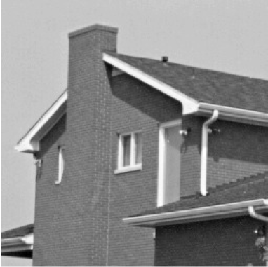
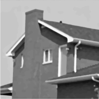
Fig. 1: Original image $\overline{x}$ (top), restored image (bottom).

In our restoration approach, the function $\mathsf{f}$ is the indicator function of the set $[0,255]^{N}$, while $\mathsf{g}_{1}\circ\mathsf{L}_{1}$ is a classical isotropic total variation regularizer, where $\mathsf{L}_{1}$ is the concatenation of the horizontal and vertical discrete gradient operators. Figs. 1–2 displays the original image, the restored image, as well as two realizations of the degraded images. The SNR for the restored image is equal to $28.1$ dB.

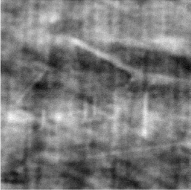
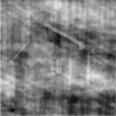
Fig. 2: Degraded image 1 (SNR = $0.14$ dB) (top), and degraded image 2 (SNR = $12.0$ dB) (bottom).

Fig. 3 shows the convergence behavior of the algorithm. In these experiments, we have chosen

$$(\forall n\in\mathbb{N})\quad\begin{cases}m_{n}=n^{1.1}\\ \lambda_{n}=(1+(n/500)^{0.95})^{-1}.\end{cases}$$ (22)

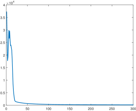
Fig. 3: $\|x_{n}-x_{\infty}\|$ versus the iteration number $n$.

5 Conclusion

We have proposed two stochastic proximal splitting algorithms for solving nonsmooth convex optimization problems. These methods require only approximations of the functions used in the formulation of the optimization problem, which is of the utmost importance for solving online signal processing problems. The almost sure convergence of these algorithms has been established. The stochastic version of the primal-dual algorithm that we have investigated has been evaluated in an online image restoration problem in which the data are blurred by a stochastic point spread function and corrupted with noise.

References

-
[1]
Y. F. Atchadé, G. Fort, and E. Moulines,
“On stochastic proximal gradient algorithms,”
2014.
http://arxiv.org/abs/1402.2365 - [2] F. Bach and E. Moulines, “Non-asymptotic analysis of stochastic approximation algorithms for machine learning”, in Proc. Ann. Conf. Neur. Inform. Proc. Syst., Granada, Spain, Dec. 12-17, 2011, pp. 451–459.
- [3] H. H. Bauschke and P. L. Combettes, Convex Analysis and Monotone Operator Theory in Hilbert Spaces. Springer, New York, 2011.
-
[4]
P. Bianchi, W. Hachem, and F. Iutzeler,
“A stochastic coordinate descent primal-dual algorithm and
applications to large-scale composite optimization,” 2014.
http://arxiv.org/abs/1407.0898 - [5] A. Chambolle and T. Pock, “A first-order primal-dual algorithm for convex problems with applications to imaging,” J. Math. Imaging Vision, vol. 40, pp. 120–145, 2011.
- [6] C. Chaux, P. L. Combettes, J.-C. Pesquet, and V. R. Wajs, “A variational formulation for frame-based inverse problems,” Inverse Problems, vol. 23, pp. 1495–1518, 2007.
- [7] P. L. Combettes, “Solving monotone inclusions via compositions of nonexpansive averaged operators,” Optimization, vol. 53, pp. 475–504, 2004.
- [8] P. L Combettes, L. Condat, J.-C. Pesquet, and B. C. Vũ. “A forward-backward view of some primal-dual optimization methods in image recovery,” Proc. IEEE Int. Conf. Image Process., Paris, France, 27-30 Oct. 2014, pp. 4141–4145.
- [9] P. L. Combettes and J.-C. Pesquet, “Proximal thresholding algorithm for minimization over orthonormal bases”, SIAM J. Optim., vol. 18, pp. 1351–1376, 2007.
- [10] P. L. Combettes and J.-C. Pesquet, “Proximal splitting methods in signal processing,” in Fixed-Point Algorithms for Inverse Problems in Science and Engineering, (H. H. Bauschke et al., eds), pp. 185–212. Springer, New York, 2011.
- [11] P. L. Combettes and J.-C. Pesquet, “Primal-dual splitting algorithm for solving inclusions with mixtures of composite, Lipschitzian, and parallel-sum type monotone operators,” Set-Valued Var. Anal., vol. 20, pp. 307–330, 2012.
- [12] P. L. Combettes and J.-C. Pesquet, “Stochastic quasi-Fejér block-coordinate fixed point iterations with random sweeping,” SIAM J. Optim., vol. 25, pp. 1221–1248, 2015.
- [13] P. L. Combettes and J.-C. Pesquet, “Stochastic approximations and perturbations in forward-backward splitting for monotone operators,” Pure Appl. Funct. Anal., vol. 1, pp. 13-37, 2016.
- [14] P. L. Combettes and H. J. Trussell, “Methods for digital restoration of signals degraded by a stochastic impulse response,” IEEE Trans. Acoustics, Speech, Signal Process., vol. 37, pp. 393–401, 1989.
- [15] P. L. Combettes and B. C. Vũ, “Variable metric forward-backward splitting with applications to monotone inclusions in duality,” Optimization, vol. 63, pp. 1289–1318, 2014.
- [16] P. L. Combettes and I. Yamada, “Compositions and convex combinations of averaged nonexpansive operators,” J. Math. Anal. Appl., vol. 425, pp. 55–70, 2015.
- [17] P. L. Combettes and B. C. Vũ, “Variable metric forward-backward splitting with applications to monotone inclusions in duality,” Optimization, vol. 63, pp. 1289–1318, 2014.
- [18] P. L. Combettes and V. R. Wajs, “Signal recovery by proximal forward-backward splitting,” Multiscale Model. Simul., vol. 4, pp. 1168–1200, 2005.
- [19] L. Condat, “A primal-dual splitting method for convex optimization involving Lipschitzian, proximable and linear composite terms,” J. Optim. Theory Appl., vol. 158, pp. 460–479, 2013.
- [20] J. Duchi and Y. Singer, “Efficient online and batch learning using forward backward splitting,” J. Mach. Learn. Res., vol. 10, pp. 2899–2934, 2009.
- [21] Yu. M. Ermoliev and Z. V. Nekrylova, “The method of stochastic gradients and its application,” in Seminar: Theory of Optimal Solutions, no. 1, Akad. Nauk Ukrain. SSR, Kiev, pp. 24–47, 1967.
- [22] E. Esser, X. Zhang, and T. Chan, “A general framework for a class of first order primal-dual algorithms for convex optimization in imaging science,” SIAM J. Imaging Sci., vol. 3, pp. 1015–1046, 2010.
- [23] O. V. Guseva, “The rate of convergence of the method of generalized stochastic gradients,” Kibernetika (Kiev), vol. 1971, pp. 143–145, 1971.
- [24] B. He and X. Yuan, “Convergence analysis of primal-dual algorithms for a saddle-point problem: from contraction perspective,” SIAM J. Imaging Sci., vol. 5, pp. 119–149, 2012.
- [25] N. Komodakis and J.-C. Pesquet, “Playing with duality: An overview of recent primal-dual approaches for solving large-scale optimization problems,” IEEE Signal Process. Mag., vol. 32, pp. 31–54, 2015.
- [26] H. J. Kushner and G. G. Yin, Stochastic Approximation and Recursive Algorithms with Applications, 2nd ed. Springer, New York, 2003.
- [27] J. Konec̆ný, J. Liu, P. Richtárik, and M. Takác̆, “Minibatch semi-stochastic gradient descent in the proximal setting,” IEEE J. Selected Topics Signal Process., vol. 10, pp. 242–255, 2016.
- [28] S. Ono, M. Yamagishi, and I. Yamada, “A sparse system identification by using adaptively-weighted total variation via a primal-dual splitting approach,” in Proc. Int. Conf. Acoust., Speech Signal Process., Vancouver, Canada, 26-31 May 2013, pp. 6029–6033.
- [29] M. Pereyra, P. Schniter, E. Chouzenoux, J.-C. Pesquet, J.-Y. Tourneret, A. O. Hero, and S. McLaughlin, “A survey of stochastic simulation and optimization methods in signal processing,” IEEE J. Selected Topics Signal Process., vol. 10, pp. 224–241, 2016.
- [30] J.-C. Pesquet and A. Repetti, “A class of randomized primal-dual algorithms for distributed optimization,” J. Nonlinear Convex Anal., vol. 16, pp. 2453–2490, 2015.
- [31] H. Robbins and S. Monro, “A stochastic approximation method,” Ann. Math. Statistics, vol. 22, pp. 400–407, 1951.
-
[32]
L. Rosasco, S. Villa, and B. C. Vũ,
“Convergence of stochastic proximal gradient algorithm,” 2014.
http://arxiv.org/abs/1403.5074 - [33] L. Rosasco, S. Villa, and B. C. Vũ, “Stochastic forward-backward splitting for monotone inclusions,” J. Optim. Theory Appl., to appear.
- [34] L. Rosasco, S. Villa, and B. C. Vũ, “A stochastic inertial forward-backward splitting algorithm for multivariate monotone inclusions,” Optimization, to appear.
- [35] S. Shalev-Shwartz and T. Zhang, “Stochastic dual coordinate ascent methods for regularized loss minimization,” J. Mach. Learn. Res., vol. 14, pp. 567–599, 2013.
- [36] N. Z. Shor, Minimization Methods for Non-Differentiable Functions. Springer, New York, 1985.
- [37] L. Xiao and T. Zhang, “A proximal stochastic gradient method with progressive variance reduction,” SIAM J. Optim., vol. 24, pp. 2057–2075, 2014.
- [38] M. Yamagishi, M. Yukawa, and I. Yamada, “Acceleration of adaptive proximal forward-backward splitting method and its application to sparse system identification,” in Proc. Int. Conf. Acoust., Speech Signal Process., Prague, Czech Republic, May 22-27, 2011, pp. 4296–4299.
- [39] B. C. Vũ, “A splitting algorithm for dual monotone inclusions involving cocoercive operators,” Adv. Comput. Math., vol. 38, pp. 667–681, 2013.
- [40] B. Widrow and S. D. Stearns, Adaptive Signal Processing. Prentice-Hall, Englewood Cliffs, NJ, 1985.