Meta-learning within Projective Simulation

Abstract

Learning models of artificial intelligence can nowadays perform very well on a large variety of tasks. However, in practice different task environments are best handled by different learning models, rather than a single, universal, approach. Most non-trivial models thus require the adjustment of several to many learning parameters, which is often done on a case-by-case basis by an external party. Meta-learning refers to the ability of an agent to autonomously and dynamically adjust its own learning parameters, or meta-parameters. In this work we show how projective simulation, a recently developed model of artificial intelligence, can naturally be extended to account for meta-learning in reinforcement learning settings. The projective simulation approach is based on a random walk process over a network of clips. The suggested meta-learning scheme builds upon the same design and employs clip networks to monitor the agent’s performance and to adjust its meta-parameters “on the fly”. We distinguish between “reflexive adaptation” and “adaptation through learning”, and show the utility of both approaches. In addition, a trade-off between flexibility and learning-time is addressed. The extended model is examined on three different kinds of reinforcement learning tasks, in which the agent has different optimal values of the meta-parameters, and is shown to perform well, reaching near-optimal to optimal success rates in all of them, without ever needing to manually adjust any meta-parameter.

I Introduction

There are many different kinds of artificial intelligent (AI) schemes. These schemes differ in their design, purpose, and underlying principles AI_ModernApproach . One feature common to all non-trivial proposals is the existence of learning parameters, which reflect certain assumptions or bias about the task or environment with which the agent has to cope 2009_Metalearning_book . Moreover, as a consequence of the so-called no-free lunch theorems NFL97 , it is known that it is impossible to have a fixed set of parameters which are optimal for all task environments. In practice these parameters (which, for some schemes, may be more than a dozen, e.g. in the extended learning classifier systems wilson1995classifier ) are typically fine-tuned manually by an external party (the user), on a case-by-case basis. An autonomous agent, however, is expected to adjust its learning parameters, automatically, by itself. Such a self monitoring and adaptation of the agent’s own internal settings is often termed as meta-learning 2009_Metalearning_book ; schaul2010metalearning ; 2004_ML_Carrier .

In the AI literature the term meta-learning, defined as “learning to learn” thrun1998learning or as a process of acquiring meta-knowledge 2004_ML_Carrier ; 2009_Metalearning_book , is used in a broad sense and accounts for various concepts. These concepts are tightly linked to practical problems, two of which are mostly considered in the context of meta-learning. In the first problem meta-learning accounts for a selection of a suitable learning model for a given task 2002_Duch_InBook ; brazdil2003ranking ; zhao2006model ; adankon2009model ; AbdulrahmanEtAl:MetaSel2015 or combination of models todorovski2003combining , including automatic adjustments when the task is changed. In the second problem meta-learning accounts for automatic tuning of model learning parameters, also referred to as meta-parameters schaul2010metalearning ; Ishii2002665 ; 2003_Schweighofer_ML_in_RL ; eriksson2003evolution ; kobayashi2009 ; tokic2013 in reinforcement learning (RL) or hyperparameters bengio2000gradient ; bardenet2010surrogating ; bergstra2012random ; reif2012meta ; Thornton:2013:ACS ; smith2014recommending ; feurer2015initializing in supervised learning.

Both of these concepts of meta-learning are widely addressed in the framework of supervised learning. The problem of supervised learning model selection, or algorithm recommendation, is solved by, e.g., the k-Nearest Neighbor algorithm brazdil2003ranking , similarity-based methods 2002_Duch_InBook , meta decision trees todorovski2003combining or an empirical error criterion adankon2009model . The second problem in meta-learning, the tuning of hyperparameters, is usually solved by gradient-based optimization bengio2000gradient , grid search bardenet2010surrogating , random search bergstra2012random , genetic algorithms reif2012meta or Bayesian optimization Thornton:2013:ACS ; feurer2015initializing . Approaches to combined algorithm selection and hyperparameter optimization were recently presented in Refs. Thornton:2013:ACS ; smith2014recommending ; feurer2015initializing .

In the RL framework, where an agent learns from interacting with a rewarding environment SuttonBarto98 , the notion of meta-learning usually addresses the second practical problem, the need to automatically adjust meta-parameters, such as the discount factor, the learning rate and the exploitation–-exploration parameter Ishii2002665 ; 2003_Schweighofer_ML_in_RL ; eriksson2003evolution ; Achbany20082507 ; kobayashi2009 ; tokic2013 . In the context of RL it is also worthwhile to mention the Gödel machine 2005_Schmidhuber_Godel_machine , which is, due to its complexity, of interest predominantly as a theoretical construction in which all possible meta-levels of learning are contained in fully self-referential learning system.

In this paper we develop a simple form of meta-learning for the recently introduced model of projective simulation (PS) 2012_Briegel_PSI . The PS is a model of artificial intelligence that is particularly suited to RL problems (see 2013_Mautner_PSII ; 2014_Melnikov_PSIII ; bjerland2015projective where the PS was shown to perform well, in comparison to more standard RL machinery, on both toy- and real-world tasks such as the “grid-world”, the “mountain-car”, the “cart-pole balancing” problem and the “Infinite Mario” game, and see 2015_Melnikov_PS_Generalization where it handles infinitely large RL environments through a particular generalization mechanism). The model is physics-oriented, aiming at an embodied Understanding_Intelligence_1999 (rather than computational) realization, with a random-walk through its memory structure as its primary process. PS is based on a special type of memory, called the episodic & compositional memory (ECM), that can be represented as a directed weighted graph of basic building blocks, called clips, where each clip represents a memorized percept, action, or combinations thereof. Once a percept is perceived by the PS agent, the corresponding percept clip is activated, initiating a random-walk on the clip-network, that is the ECM, until an action clip is hit and the corresponding action is performed by the agent. This realizes a stochastic processing of the agent’s experience.

The elementary process of the PS, namely the random-walk, is an established theoretical concept, with known applications in randomized algorithms Randomized_Algorithms_1995 , thus providing a large theoretical tool box for designing and analyzing the model. Moreover, the random walk can be extended to the quantum regime, leading to quantum walks 1965_Feynman ; 1993_Aharonov ; Aharonov:2001 , in which case polynomial and even exponential improvements have been reported in e.g. hitting and mixing times Childs:2003 ; Kempe2005 ; KMOR . The results in the theory of quantum walks suggest that improvements in the performance of the PS may be achievable by employing these quantum analogues. Recently, a quantum variant of the PS (envisioned already in 2012_Briegel_PSI ) was indeed formalized and shown to exhibit a quadratic speed-up in deliberation time over its classical counterpart 2014_Paparo_QPS ; dunjko2015quantum ; friis2015coherent .

From the perspective of meta-learning, the PS is a comparatively simple model with few number of learning parameters 2013_Mautner_PSII . This suggests that providing the PS agent with a meta-learning mechanism may be done while maintaining its overall simplicity. In addition to simplicity, we also aim at structural homogeneity: the meta-learning component should be combined with the basic model in a natural way, with minimal external machinery. In accordance with these requirements, the meta-learning capability which we develop here is based on supplementing the basic ECM network, which we call the base-level ECM network, with additional meta-level ECM networks that dynamically monitor and control the PS meta-parameters. This extends the structure of the PS model from a single network to several networks that influence each other.

In general, when facing the challenge of meta-learning in RL, one immediately encounters a trade-off between efficiency (in terms of learning times) and success rates (in terms of achievable rewards), on the one side, and flexibility on the other side (as pointed out, e.g., also in 2007_AI_Magazine_Anderson ). Humans, for example, are extremely flexible and robust to changes in the environment, but are not very efficient and reach sub-optimal success rates. Machines, on the other hand, can learn fast and perform optimally at a given task (or a family of tasks), yet fail completely on another. Clearly, to achieve a level of robustness, machines would have to repeatedly revise and update their internal design, i.e. to meta-learn, a process which necessarily takes time. Moreover, reaching optimal success rates in certain tasks, may require an over-fitting of the scheme’s meta-parameters, which might harm its success in other tasks. It can therefore be expected that any form of meta-learning (which improves the flexibility of the model), may do so at the expense of the model’s efficiency and (possibly even) success rates, and we will observe this inclination also in our work.

Another aspect of meta-learning which we highlight throughout the paper is the underlying principles that govern the agent’s internal adjustment. Here, we distinguish between two different (sometimes complementary) alternatives which we call reflexive adaptation and adaptation through learning. Informally, by reflexive adaptation we mean that the agent’s meta-parameters are adjusted via a fixed recipe (which may or may not be deterministic), which takes into account only the recent performance of the agent, while ignoring the rest of the agent’s history. Essentially, this amounts to adaptation without a need for additional memory. An example for such a reflexive adaptation approach for meta-learning can be found in 2003_Schweighofer_ML_in_RL where the fundamental RL parameters, namely, the learning rate $\alpha$, the exploitation-exploration parameter $\beta$, and the discount factor $\gamma$ are tuned according to predefined equations; In contrast, an agent which adapts its parameter through learning, exploits to that end its entire individual experience. Accordingly, adaptation through learning does require an additional memory. In this work we consider both kinds of approaches.

The paper is structured as follows: Section II shortly describes the PS model including its meta-parameters. Section III demonstrates the advantages of meta-learning, by considering explicit task scenarios where the PS model has different optimal values of the meta-parameters. In Section IV we present the proposed meta-learning design and explain how it combines with the basic model. The model is then examined and analyzed through simulations in Section V, where the performance of the meta-learning PS agent is evaluated in three different types of changing environments. Throughout this section the proposed meta-learning scheme is further compared to other, more naive, alternatives of meta-learning schemes. Finally, Section VI concludes the paper and discusses some of its open questions.

II The PS model

For the benefit of the reader we first give a short summary of the PS; for a more detailed description, including recent developments see 2012_Briegel_PSI ; 2013_Mautner_PSII ; 2014_Melnikov_PSIII ; 2015_Melnikov_PS_Generalization ; bjerland2015projective . The central component of the PS model is the episodic $\&$ compositional memory (ECM), formally a network of clips. The possible clips include percept clips (representing a percept) and action clips (representing an action), but can also include the representations of various combinations of percept and action sequences (thus representing e.g. an elapsed exchange between the agent and environment, or subsets of the percept space as occurring in the model of PS with generalization 2015_Melnikov_PS_Generalization ). Within the ECM, a clip $c_{i}$ may be connected to clip $c_{j}$ via a weighted directed edge, with a corresponding time-dependent real positive weight $h^{(t)}(c_{i},c_{j})$ (called $h$-value), which is larger than or equal to its initial value of $h_{0}=1$.

The deliberation process of the agent corresponds to a random walk in the ECM, where the transition probabilities are proportional to the $h-$values. More specifically, upon encountering a percept, the clip corresponding to that percept is activated, and a random walk is initiated. The transition probability from clip $c_{i}$ to $c_{j}$ at time step $t$, corresponds to the re-normalized $h$-values:

$$p^{(t)}(c_{j}|c_{i})=\dfrac{h^{(t)}(c_{i},c_{j})}{\sum_{k}h^{(t)}(c_{i},c_{k})}.$$ (1)

The random walk is continued until an action clip has been hit, upon which point the corresponding action is carried out.

The learning aspect of the PS agent is achieved by the dynamic modification of the $h-$values, depending on the response of the environment. Formally, at each time-step, the $h$-values of the edges that were traversed during the preceding random walk are updated as follows:

$$h^{(t+1)}(c_{i},c_{j})=h^{(t)}(c_{i},c_{j})-\gamma(h^{(t)}(c_{i},c_{j})-1)+\lambda,$$ (2)

where $0\leq\gamma\leq 1$ is a damping parameter and $\lambda$ is a non-negative reward given by the environment. The $h$-values of the edges which were not traversed during the preceding random walk are not rewarded (no addition of $\lambda$), but are nonetheless damped away toward their initial value $h_{0}=1$ (by the $\gamma$ term). With this update rule in place, the probability to take rewarded actions is increased with time, that is, the agent learns.

The damping parameter $\gamma$ is a meta-parameter of the PS model. The higher it is, the faster the agent forgets its knowledge. For certain settings, introducing additional parameters to the ECM network can lead to better learning performance. A particularly useful generalization is the “edge glow” mechanism, introduced to the model in 2013_Mautner_PSII . Here, an additional time-dependent variable $0\leq g\leq 1$ is attributed to each edge of the ECM, and a term depending on its value is added to the update rule of the $h-$values:

$$h^{(t+1)}(c_{i},c_{j}) = h^{(t)}(c_{i},c_{j})-\gamma(h^{(t)}(c_{i},c_{j})-1)$$ (3)

$$+ g^{(t)}(c_{i},c_{j})\lambda.$$

This update rule holds for all edges, so that edges which were not traversed still may end up being enhanced, proportional to their $g-$value. The $g-$value dynamically changes. Each time an edge is traversed, its $g$-value is set to $g=1$, and dissipates in the following time steps with a rate $\eta$:

$$g^{(t+1)}(c_{i},c_{j})=g^{(t)}(c_{i},c_{j})(1-\eta).$$ (4)

The $\eta$ parameter is thus another meta-parameter of the model.

The decay of the $g$-values ensures that the reward effects the edges traversed at different points in time, to a different extent. In particular, recently traversed edges are enhanced more (after a rewarding step), relative to edges traversed in the more remote past. The $\eta$ parameter controls the strength of this temporal dependence. For instance, a low value of $\eta$ implies that the edges which were traversed a while back in the past will nonetheless be enhanced. In contrast, by setting $\eta=1$, only the last traversed path is enhanced in which case the update rule reverts back to Eq. (2).

The glow mechanism thus establishes temporal correlations between percept-action pairs, and enables the agent to perform well also in settings where the reward is delayed (e.g. in the grid-world and the mountain-car tasks 2014_Melnikov_PSIII ) and/or contingent on more than just the immediate history of agent-environment interaction (such as in the $n$-ship game, as presented in 2013_Mautner_PSII ).

The basic variant of the PS model (so-called two-layered variant) can be formally contrasted to more standard RL schemes, where it closely resembles the SARSA algorithm rummery1994line . An initial analysis of the relationship of the two models was given in 2015_Melnikov_PS_Generalization . Readers familiar with the SARSA model may benefit from the observation that the functional roles of the $\alpha$ and $\gamma$ parameters in SARSA are closely matched by the $\gamma$ and $\eta$ parameters of the PS, respectively. However, as the PS is explicitly not a state-action value function-based model, the analogy is not exact. For more details we refer the interested reader to 2015_Melnikov_PS_Generalization . In the following section, we describe the behaviour of the PS model, and the functional role of its meta-parameters in greater detail.

III Advantages of Meta-learning

The basic memory update mechanism of the PS, as captured by Eq. (3)-(4) has two meta-parameters, namely the damping parameter $\gamma$, and the glow parameter $\eta$. In what follows, we examine the role of these parameters in the learning process of the agent. We then demonstrate, through examples, that for none of these parameters there is a unique value that is universally optimal, i.e. that different environments induce different optimal $\gamma$ and $\eta$ values. These examples provide direct motivation for introducing a meta-learning mechanism for the PS model.

III.1 Damping: the $\gamma$ parameter

The damping parameter $0\leq\gamma\leq 1$ controls the forgetfulness of the agent, by continuously damping the $h$-values of the clip network. A direct consequence of this is that a non-zero $\gamma$ value bounds the $h$-values of the clip network to a finite value, which in turn limits the maximum achievable success probability of the agent. As a result, in many typical tasks considered in the RL literature (grid-world, mountain-car, and tic-tac-toe, to name a few), in which the environments are consistent, i.e. not changing, the optimal performance is achieved without any damping, that is by setting $\gamma=0$.

However, when the environment does change, the agent may need to modify its “action pattern”, which implies varying the relative weights of the $h$-values. Presetting a finite $\gamma$ parameter would then quicken the agent’s learning time in the new environment, at the expense of reaching lower success probabilities, as demonstrated and discussed in Ref. 2012_Briegel_PSI . This gives rise to a clear trend: The higher the value of $\gamma$, the faster is the relearning in a changing environment, and the lower is the agent’s asymptotic success probability.

The trade-off between learning time and success probability in changing environments can be demonstrated on the invasion game 2012_Briegel_PSI example. The invasion game is a special case of the contextual multi-armed bandit problem Bandits05 and has no temporal dependence. In this game an agent is a defender and should try to block an attacker by moving in the same direction (left or right) with the attacker. Before making a move, the attacker shows a symbol (“$\Leftarrow$” or “$\Rightarrow$”), which encodes its future direction of movement. Essentially, the agent has to learn where to go for every given direction symbol. Fig. 1 illustrates how the PS agent learns by receiving rewards for successfully blocking the attacker. Here, during a phase of 250 steps, the attacker goes right (left) whenever it shows a right (left) symbol, but then, at the second phase of the game, the attacker inverts its rules, and goes right (left) whenever it shows left (right). It is seen that higher values of $\gamma$ yield lower success probabilities, but allow for a faster learning in the second phase of the game.

Figure 1: (Color online) Invasion game: The attacker inverts its strategy after 250 steps. The agent’s average success probability is plotted as a function of number of trials (games). A trade-off between success probability and relearning time is depicted for different $\gamma$ values. An optimal value of $\eta=1$ is used. The simulation was done by averaging over $10^{6}$ agents. Adapted from 2012_Briegel_PSI .

To illustrate further the slow-down of the learning time in a changing environment when setting $\gamma=0$, Fig. 2 shows the average success probability of the basic PS agent in the invasion game as a function of number of trials, on a log scale. Here the attacker inverts its rules whenever the agent reaches a certain success probability (here set to 0.8). We can see that the time that the agent needs to learn at each phase grows exponentially in the number of the changes of the phases, requiring more and more time for the agent to learn, so that eventually, for any finite learning time, there will be a phase for which the agent fails to learn.

Figure 2: Invasion game: The attacker inverts its strategy whenever the agent’s success probability reaches 0.8. The agent’s performance is plotted as a function of number of trials on a log scale, demonstrating learning times that increase exponentially with the number of inversions. The simulation was done with a single agent, where the success probabilities were extracted directly from the agent’s base-level ECM network. Meta-parameters: $\gamma=0$, $\eta=1$.

Setting a zero damping parameter in changing environments may even be more harmful for the agent than merely increasing its learning time. To give an example, consider an invasion game, where the attacker inverts its rules every fixed finite number of steps. Without damping, the agent will only be able to learn a single set of rules, while utterly failing on the inverted set. This is shown in Fig. 3.

Figure 3: Invasion game: The attacker changes its strategy every 500 steps. The agent’s average success probability is plotted as a function of number of trials, demonstrating that only one of the two set of the attacker’s strategy can be learned. Moreover, the performance of the agent, averaged over the two phases, converges to the performance of a random agent. The simulation was done by averaging over 100 agents, where for each agent the success probabilities were extracted directly from its base-level ECM network. Meta-parameters: $\gamma=0$, $\eta=1$.

The performance of the PS agent in the considered examples, shown in Figs. 1 – 3, suggests that it is important to raise the $\gamma$ parameter whenever the environment changes (the performance drops down) and set it to zero whenever the performance is steady. As we will show in Section IV.2 this adjustment can be implemented by means of reflexive adaptation. However the reflexive adaptation of the $\gamma$ parameter makes meta-learning less general, because it fixes the rule of the parameter adjustment. To make the PS agent more general we will implement $\gamma$ adaptation also through learning, which gives the agent the possibility to learn the opposite rule, i.e. to decrease $\gamma$ whenever the agent’s performance goes down.

So far we assumed that the glow mechanism is turned off by setting $\eta=1$, which is optimal for the invasion game. The same holds in all environments where the rewards depend only on the current percept-action pair, with no temporal correlations to previous percepts and actions. In the next section, however, we look further into scenarios where such temporal correlations do exist, and study their influence on the optimal $\eta$ value.

III.2 Glow: the $\eta$ parameter

In task environments where reward from an environment is a consequence of a series of decisions made by an agent, it is vital to ensure that not only the last action is rewarded, but the entire sequence of actions. Otherwise, these previous actions, which eventually led to a rewarded decision, will not be learned. As described in Sec. II, rewarding a sequence of actions is done in the PS model by attributing a time dependent $g$-value to each edge of the clip network and rewarding the edge with a reward proportional to its $g$-value. Once an edge is excited, its $g$-value is set to $g=1$, whereas all other $g$-values decay with a rate $\eta$, which essentially determines the extent to which past actions are rewarded. As we show next, the actual value of the $\eta$ parameter plays a crucial role in obtaining high average reward, its optimal value depends on the task, and finding it is not trivial.

Here we study the role of the $\eta$ parameter in the $n$-ship game example, introduced in 2013_Mautner_PSII . In this game $n$ ships arrive in a sequence, one by one, and the agent is capable of blocking them. If the agent blocks one or several ships out of the first $n-1$ ships, it will get a reward of $\lambda_{\mathrm{min}}=1$ for each ship immediately after blocking it. If, however, the agent will refrain from blocking the ships, although there is an immediate reward for that, it will get a larger reward of $\lambda_{\mathrm{max}}=5\times(n-1)$ for blocking only the last, $n$-th ship. In this scenario the optimal strategy differs from the greedy strategy of collecting immediate rewards, because the reward $\lambda_{\mathrm{max}}$ is larger than the sum of all the small rewards that can be obtained during the game.

The optimal strategy in the described game can be learned by using the glow mechanism and by carefully choosing the $\eta$ parameter. The optimal $\eta$ value depends on the number of ships $n$, as shown in Fig. 4, where the dependence of the average reward received during the game on the $\eta$ parameter is plotted for each $n\in\{2,3,4\}$. It is seen that as the number of $n$ ships grows, the best average reward is obtained using a smaller $\eta$ value, i.e. the optimal $\eta$ value decreases. This makes sense as a smaller $\eta$ value leads to larger sequences of rewarded actions.

Figure 4: (Color online) $n$-ship game: The dependence of the performance on the $\eta$ parameter is shown for different $n$. The performance is evaluated by an average reward gained during the $10^{6}$-th game. The simulation was done by averaging over $10^{3}$ agents. The $\gamma$ parameter was set to $10^{-4}$. Adapted from 2013_Mautner_PSII .

The simulations of the $n$-ship game shown in Fig. 4 emphasize the importance of setting a suitable $\eta$ value. In other, more involved scenarios, such a dependency may be more elusive, making the task of setting a proper $\eta$ value even harder. An internal mechanism that dynamically adapts the glow parameter according to the (possibly changing) external environment would therefore further enhance the autonomy of the PS agent. In Section IV.1 we will show how to implement this internal mechanism by means of adaptation through learning.

IV Meta-learning within PS

To enhance the PS model with a meta-learning component, we supplement the base-level clip-network (ECM) with additional networks, one for each meta-parameter $\xi$ (where $\xi$ could be, e.g. $\gamma$ or $\eta$). Each such meta-level network, which we denote by ECM_ξ obeys the same principle structure and dynamic as the base-level ECM network as described in Section II: it is composed of clips, its activation initiates a random-walk through the clips until an action-clip is hit, and its update rule is given by the update rule of Eq. (2), albeit with a different internal reward:

$$h_{\xi}^{(t+1)}(c_{i},c_{j})=h_{\xi}^{(t)}(c_{i},c_{j})-\gamma_{\xi}(h_{\xi}^{(t)}(c_{i},c_{j})-1)+\lambda_{\xi}.\leavevmode\nobreak\ \leavevmode\nobreak\ \leavevmode\nobreak\ \leavevmode\nobreak\$$ (5)

The meta-level ECM networks we consider in this work are two-layered, with a single percept-clip and several action-clips. The action clips of each meta-level network determine the next value of the corresponding meta-parameter. This is illustrated schematically in Fig. 5.

Figure 5: A schematic two-layered meta-level ECM_ξ network, whose actions control the value of a general meta-parameter $\xi$.

While the base-level ECM network is activated at every interaction with the environment (where each percept-action pair of the agent counts as a single interaction), a meta-level ECM_ξ network is activated only every $\tau_{\xi}$ interactions with the environment. Following each activation, an action-clip is encountered and the meta-parameter $\xi$ (thus either $\gamma$ or $\eta$) is updated accordingly. At the end of each such $\tau_{\xi}$ time window the meta-level network receives an internal reward $\lambda_{\xi}$ which reflects how well the agent performed during the past $\tau_{\xi}$ interactions, or time steps, compared to the performance during the previous $\tau_{\xi}$ time window. This allows a statistical evaluation of the agent’s performance in the last $\tau_{\xi}$ time window.

Specifically, we consider the quantity

$$\Lambda_{\xi}(T)=\sum_{t=T-\tau_{\xi}+1}^{T}\lambda^{(t)},$$ (6)

which accounts for the sum of rewards that the agent has received from the environment in the $\tau_{\xi}$ steps before the end of the time step $T$. The internal reward $\lambda_{\xi}$ is then set by comparing two successive values of such accumulative rewards:

$$\lambda_{\xi}=\mathop{\mathrm{sgn}}\left(\Delta_{\xi}\right)$$ (7)

where $\Delta_{\xi}(T)=\frac{\Lambda_{\xi}(T)-\Lambda_{\xi}(T-\tau_{\xi})}{\max\{\Lambda_{\xi}(T),\Lambda_{\xi}(T-\tau_{\xi})\}}$ is the normalized difference in the agent’s performance between two successive time windows, before time step $T$. In short, the meta-level ECM_ξ network is rewarded positively (negatively) whenever the agent performs better (worse) in the latter time window (implementation insures that the corresponding $h$-values do not go below 1). The normalization plays no role at this point, however the numerical value of $\Delta_{\xi}$ will matter later on. When there is no change in performance ($\Delta_{\xi}(T)=0$) the network is not rewarded.

The presented design requires the specification of several quantities for each meta-level ECM_ξ network, including: the time window $\tau_{\xi}$, the number of its actions and the meaning of each action. In what follows we specify these choices for both the $\eta$ and the $\gamma$ meta-level networks.

IV.1 The glow meta-level network (ECM_η) – adaptation through learning only

The glow meta-level network (ECM_η) we use in this work is depicted in Fig. 6. The network is composed of a single percept ($S_{\eta}=1$) and $A_{\eta}=10$ actions which correspond to setting the $\eta$ parameter to one of 10 values from the set $\{0.1,0.2,\ldots,1\}$. The internal glow network is activated every $\tau_{\eta}$ times steps. This time window should be large enough so as to allow the agent to gather reliable statistics of its performance. It is therefore sensible to set $\tau_{\eta}$ to be of the order of the learning time of the agent, that is the time it takes the agent to reach a certain fraction of its asymptotic success probability (see also 2013_Mautner_PSII ). The learning time of the PS was shown in 2013_Mautner_PSII to be linear in the number of percepts $S$ and actions $A$ in the base-level network. We thus set the time window to be $\tau_{\eta}=N_{\eta}SAS_{\eta}A_{\eta}$, which is also linear with the number of percepts $S_{\eta}$ and actions $A_{\eta}$ of the meta-level network. Here $N_{\eta}$ is a free parameter; the higher its value, the better the statistics the agent gathers. In this work, we set $N_{\eta}=30$ throughout, for all the examples we study.

Figure 6: The glow meta-level network (ECM_η): The specific realization employed in this work.

The $h_{\eta}$-values of the $\eta$-network are updated through internal rewarding as described, and the PS agent learns with time what the preferable $\eta$ values in a given scenario are. The preferable $\eta$ values are further adjusted to account for changes in the environment. These continuous adjustments of the $\eta$-network then allow the PS agent to adapt to new environments by learning.

IV.2 The damping meta-level network (ECM_γ) – combining reflexive adaptation with adaptation through learning

The second meta-learning network, the damping meta-level network (ECM_γ), is presented in Fig. 7. It is composed of only two actions which correspond to updating the $\gamma$ parameter by using one of two functions according to the following rules:

$$\text{Rule I:}\quad\gamma\leftarrow f_{\mathrm{I}}(\gamma)=(1-|\tilde{\Delta}_{\gamma}|)\gamma+\frac{|\tilde{\Delta}_{\gamma}|-\tilde{\Delta}_{\gamma}}{2}$$ (8)

and

$$\text{Rule II:}\quad\gamma\leftarrow f_{\mathrm{II}}(\gamma)=(1-|\tilde{\Delta}_{\gamma}|)\gamma+\frac{|\tilde{\Delta}_{\gamma}|+\tilde{\Delta}_{\gamma}}{2}$$ (9)

where $\tilde{\Delta}_{\gamma}=\frac{\Delta_{\gamma}+C_{\gamma}}{1+C_{\gamma}}$ and $\Delta_{\gamma}$ is defined after Eq. (7). Rule I invokes a reflexive increase of the $\gamma$ parameter when the agent’s performance deteriorates, and a reflexive decrease when the performance improves. This rule (“natural rule”) is natural for typical RL scenarios: a drop of performance is assumed to signify a change in the environment, at which point the agent should do well to forget what it learned thus far, and focus on exploring new options - in the PS both are achieved by the increase of $\gamma$. In contrast, if the environment is in a stable phase, as the agent learns, the performance improves, causing $\gamma$ to decrease, which will lead to optimal performance. Rule II (“opposite rule”) is chosen to do exactly the opposite, namely performance increase causes the agent to forget. Our main purpose for the introduction of this rule is to demonstrate the flexibility of the meta-learning agent to learn even the correct strategy of updating $\gamma$. Although in all the environments which are typically considered in literature, and in this work, the natural rule is the better choice, and thus could in principle be hard-wired, our agent is challenged to learn even this. The role of $C_{\gamma}$ parameter, which we set to $C_{\gamma}=0.2$ throughout this work, is to avoid unwanted increase of $\gamma$ under statistical fluctuations. Note that the functions in Eqs. (8) and (9) ensure that $\gamma\in[0,1]$.

Figure 7: The damping meta-level network (ECM_γ): The specific realization employed in this work.

The described $\gamma$-network is activated every $\tau_{\gamma}=N_{\gamma}\tau_{\eta}$ steps, where $\tau_{\eta}$ is the time window of the glow network as defined above, and where $N_{\gamma}$ is a free parameter of the $\gamma$-network, which we set it to $N_{\gamma}=5$ throughout the paper. The agent first learns an estimate of the range of an optimal $\eta,$ and changes $\gamma$ afterwards. This is assured by choosing the time window for the $\gamma$-network larger than for the $\eta$-network. This relationship between the time windows $\tau_{\gamma}$ and $\tau_{\eta}$ is required in order for the PS agent to gain a meaningful statistics during $\tau_{\gamma}$ steps. Otherwise, if $\eta$ is not learned first, the agent’s performance will significantly fluctuate, leading to erratic changes of $\gamma$ through the reflexive adaptation rule. Note that large fluctuations in $\gamma$ yield very poor learning results as even moderate values of $\gamma$ lead to a rapid forgetting of the agent.

The meta-learning by the ECM_γ network is realized as follows. Starting from an initially random value, the $\gamma$ parameter is adapted both via direct learning in the $\gamma$-network and via reflexive adaptation through rule I or rule II. Given that the overall structure of the environment was learned (i.e. whether the natural rule I or opposite rule II is preferable), $\gamma$ is henceforth adapted reflexively. These reflexive rules reflect an a-priory knowledge about what strategy is preferable in given environments. We note that the $\gamma$ parameters could be learned without such reflexive rules, by using networks which directly select the $\gamma$ values (like in the case of the $\eta$ network), however such approaches have shown to be much less efficient. In general, reflexive adaptation of the meta-parameters is preferable to adaptation through learning as it is simpler. The need for learning adaptation arises when the landscape of optimal values of the meta-parameters is not straightforward, as is the case for the $\eta$ parameter, as illustrated in Fig. 4.

V Simulations

To examine the proposed meta-learning mechanism we next evaluate the performance of the meta-learning PS agent in several environments, namely the invasion game, the $n$-ship game and variants of the grid-world setting. These environments were chosen because of their different structures, which exhibit different optimal damping and glow parameters. The goal is that the PS agent will adjust its meta-parameters properly, so as to cope well with these different tasks. To challenge the agent even further, each of the three environments will suddenly change, thereby forcing the agent to readjust its parameters accordingly. Critically, for all tasks the same meta-level networks are used, along with the same choice of free parameters ($N_{\eta}=30$, $N_{\gamma}=5$, and $C_{\gamma}=0.2$), as described in Sections IV.1-IV.2.

To demonstrate the role of the meta-learning mechanism, we compare the performance of the meta-learning PS agent to the performance of the PS agent without this mechanism. Without the meta-learning the PS agent starts the task with random $\gamma$ and $\eta$ parameters and does not change them afterwards. To show the importance of learning the optimal $\eta$ parameter (which may not be as obvious as for the case of $\gamma$) we construct a second reference PS agent for comparison, which uses the $\gamma$-network to adjust the $\gamma$ parameter, but takes a random choice out of the possible $\eta$-actions in the $\eta$-network.

V.1 The invasion game

We start with the simplest task: the invasion game (see Section III.1). As before, the agent is rewarded with $\lambda=1$ whenever it manages to block the attacker and it has to learn whether the attacker will go left or right, after presenting one of two symbols. We consider, once again, the scenario in which the attacker switches between two strategies every fixed number of trials. In one phase of the game it goes left (right) after showing a left (right) symbol, whereas in the other phase it does the opposite. This is repeated several times. The task of the agent is to block the attacker regardless of its strategy. We recall that in such a scenario (see Fig. 3) the basic PS agent with fixed meta-parameters ($\gamma=0,\eta=1$) can only cope with the first phase, but fails completely at the second.

Fig. 8 (a) shows in solid blue the performance of the meta-learning PS agent, in terms of average success probabilities, in this changing invasion game. Here each phase lasts $1.2\times 10^{5}$ steps, and the attacker changes its strategy 20 times. It is seen that with time the average success probability of the PS agents increases towards optimal values and that the agents manage to block the attacker equally well for both of its strategies. This performance is achieved due to meta-learning of the $\gamma$ and $\eta$ parameters, the dynamics of which are shown in solid blue in Fig. 8 (b) and (c), respectively. It is seen in Fig. 8 (b) that after some time and several phase changes, the value of the $\gamma$ parameter raises sharply whenever the attacker changes its strategy, and decays toward zero during the following phase. This allows the agent to rapidly forget its knowledge of the previous strategy and then to learn the new one. Fig. 8 (c) shows the $\eta$ parameter dynamics. As explained in Section III.2 the optimal glow value for the invasion-game is $\eta=1$, as the environment induces no temporal correlations between previous actions and rewards. The meta-learning agent begins with an

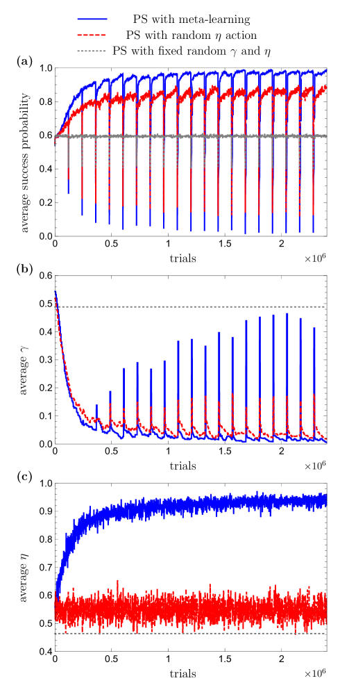
Figure 8: (Color online) Invasion game: The attacker inverts its strategy every $1.2\times 10^{5}$ steps. Three types of PS agents are depicted: with full meta-learning capability (in solid blue), with adjusted $\gamma$ value but with $\eta$ value that is chosen randomly from the ECM_η network (in dashed red), and agents whose $\gamma$ and $\eta$ values are fixed to random values, each agent with its own values (in dotted gray). Top: The performances of the different agents are shown as a function of trials; Middle: The average $\gamma$ value is shown as a function of trials; Bottom: The average $\eta$ value is shown as a function of trials. The simulations were done by averaging over 100 agents, where for each agent the success probabilities were extracted directly from its base-level ECM network.

$\eta$-network that has a uniform action probability. Yet, with time, its meta-level ECM_η network learns and the average $\eta$ parameter approaches the optimal value of $\eta=1$.

To show the advantage of the meta-learning networks we next consider the performance of agents without this mechanism. First, we look at the performance of a PS agent with fixed random $\gamma$ and $\eta$ parameters as shown in Fig. 8 (a) in dotted gray. It is seen that on average, such an agent performs rather poor, with an average success rate of $0.6$. This can be expected, as most of the $\gamma$ and $\eta$ values are in fact harmful for the agent’s success. The average value of each parameter goes to $0.5$ as depicted in Fig. 8 (b) for the $\gamma$ parameter and in Fig. 8 (c) for the $\eta$ parameter in dotted gray (the slight deviation from $0.5$ is due to finite sample size).

A more challenging comparison is shown in Fig. 8 (a) in dashed red, where the agent adjusts its $\gamma$ parameter exactly like the meta-learning one, but uses an $\eta$-network (the same one as the meta-learning agent) that does not learn or update. It is seen that such an intermediate agent can already learn both phases to some extent, but does not reach optimal values. This is because small $\eta$ values – corresponding to sustained glow over several learning cycles – are harmful in this case. The dynamics of the parameters of this PS agent are shown in Fig. 8 (b) and (c) in dashed red, where $\gamma$ behavior is similar to the one of the meta-learning agent, and the average $\eta$ fluctuates around $\eta=0.55$, which is the average value of the $10$ possible actions in the $\eta$-network.

In this example we encounter for the first time the trade-off between flexibility and learning time. The meta-learning agent exhibits high flexibility and robustness, as it manages to repeatedly adapt to changes in the environment. However, this comes with a price: the learning time of the agent slows down and the agent requires millions of trials to master this task. This is, however, to be expected. Not only that the agent has to learn how to act in a changing environment, but it must also learn how to properly adapt its meta-parameters, and the latter occurs at the time-scales of $\tau_{\gamma}=6000$ elementary cycles. The agent begins with no bias whatsoever regarding its a action pattern or its $\gamma$ and $\eta$ parameters. Furthermore, the agent begins with no a-priory knowledge regarding the inherent nature of the rewarding process of the environment: is it a typical environment (where the agent should prefer the natural rule), or is it an untypical environment which ultimately rewards random behavior (where the opposite rule will do better)? This too needs to be learned. Fig. 9 shows the average probability of choosing rule I (Eq. (8)) in the $\gamma-$network as a function of trials. It is seen that with time the $\gamma-$network chooses to update the $\gamma$ parameter according to rule I with increasing probability, reflecting the fact that in this setup the environment acts indeed according to the natural rule.

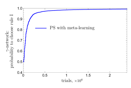
Figure 9: Invasion game: The attacker inverts its strategy every $1.2\times 10^{5}$ steps as in Fig. 8. The performance of the $\gamma$-network of the meta-learning PS is shown as a function of trials, in terms of the probability to choose rule I (see Eq. 8). The simulation was done by averaging over 100 agents.

V.2 The $n$-ship game

In the $n$-ship game (see Section III.2) the environment rewards the agent depending on its previous actions. In what follows we consider a dynamic $n$-ship game, that is we allow $n$ to change with time. In particular, the environment starts with $n=1$ (where no temporal correlations exist) and increases the number of ships $n$ by one, every $3.5\times 10^{5}\times n$ steps. As explained in Section III.2 each $n$-value requires a different glow parameter $\eta$. This scenario therefore poses the challenge of continuously adjusting the glow parameter.

Fig. 10 (a) shows in solid blue the performance of the meta-learning PS agent in this changing $n$-ship game. The best possible reward is indicated by a dashed blue horizontal line, and it is seen that such agents learn to perform optimally, for all number of ships $n$. This success is made possible by the meta-learning mechanism.

First, the $\gamma$ parameter is adjusted, such that the agent forgets whenever its performance decrease and vice versa (see Eq. (8)). Here we assume that the $\gamma$-network already learned in previous stages that the environment follows the natural rule (we used an h-value ratio of $10^{5}$ to $1$ for rule I). This $\gamma$-network leads to a dynamics of the average $\gamma$ parameter shown in Fig. 10(b) in solid blue. It is seen that whenever the environment changes, the $\gamma$ parameter increases, thereby allowing the agent to forget its previous knowledge. A slow decrease of the damping parameter makes it then possible for the agent to learn how to act in the new setup.

Second, the glow parameter $\eta$ is adjusted dynamically. Fig. 10 (c) shows the probability distribution of choosing each action of the $\eta$-network at the end of each phase. It is seen that as $n$ grows, the $\eta$-network learns to choose a smaller and smaller glow parameter value, which allows the back propagation of the reward from the final ship to the first $n-1$ ships. A similar trend was observed in Fig. 4 where larger $n$ values result with smaller

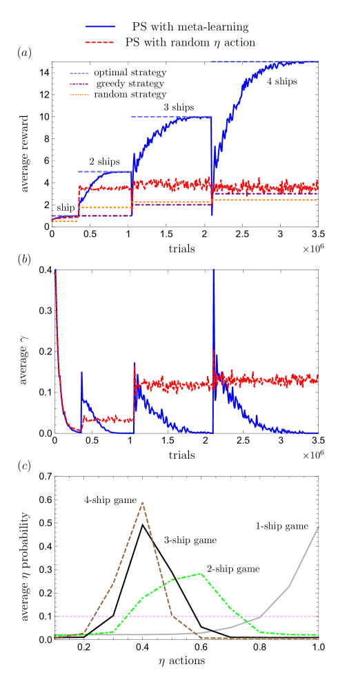
Figure 10: (Color online) n-ship game: The number of ships $n$ increases from one to four. Each phase lasts for $3.5\times 10^{5}\times n$ trials. Two types of PS agents are depicted: with full meta-learning capability (in solid blue), and with adjusted $\gamma$ value but with $\eta$ value that is chosen randomly from the ECM_η network (in dashed red). Top: The performance of the two different agents is shown as a function of trials in terms of average reward. For each phase the average reward of the optimal strategy, a greedy strategy and a fully random one is plotted in dashed light-blue, dotted-dashed purple, and dotted orange, respectively; Middle: The average $\gamma$ values of the two different kinds of agents are shown as a function of trials; Bottom: For the meta-learning PS agent the probability to choose each of the 10 $\eta$-actions is plotted at the end of each phase in a different plot. Connecting lines are shown to guide the eyes. The simulations were done by averaging over 100 agents, where for each agent the average reward was extracted directly from its base-level ECM network.

optimal $\eta$ values. As shown in Fig. 10 (c) the meta-learning PS agent essentially captures the same knowledge in its $\eta$-network. Yet, this time the knowledge is obtained through the agent’s experience, rather than by an external party.

The PS agent without the meta-learning is not able to achieve similar performance. Performance of an agent with fixed random $\gamma$ and $\eta$ is poor and not shown, because its behavior was close to a random strategy (dotted orange horizontal lines in Fig. 10 (a)). This performance is expected, because most of the values are harmful for the agent’s success. We only show the more challenging comparison (dashed red in Fig. 10), where the agent adjusts its $\gamma$ parameter exactly like the meta-learning one, but uses an $\eta$-network (the same one as the meta-learning agent) which does not learn or update. It is seen that for $n=1$ such an intermediate agent can cope with the environment, but that for higher values of $n$ it fails to reach the optimal performance because of a random $\eta$ parameter, and achieves only a mixture of a greedy strategy (dot-dashed purple horizontal lines) and an optimal strategy (dashed light blue horizontal lines).

V.3 The grid-world task

As a last example, we consider a benchmark problem in the form of the grid-world setup as presented in Ref. sutton1990integrated . This is a delayed-reward scenario, where the agent walks through a maze and gets rewarded with $\lambda=1$ only when it reaches its goal. At each position, the agent can move in one of four directions: left, right, up, or down. Each move counts as a single step. Reaching the goal marks the end of the current trial and the agent is then reset to its initial place, to start another round. The basic PS agent was shown to perform well in this benchmark task 2014_Melnikov_PSIII . Here, to challenge the new meta-learning scheme we situate the agent in three different kinds of grid-worlds: (a) The basic grid-world of Ref. sutton1990integrated , illustrated in the left part of Fig. 11; (b) The same sized grid-world with some of the walls positioned differently, as shown in the middle part of Fig. 11; and (c) The original grid-world, but with an additional small distracting reward $\lambda_{\min}=\frac{1}{3}$, placed only 12 steps from the agent, shown in the right part of Fig. 11. The game then ends either when the big reward $\lambda_{\max}=1$ or the small reward $\lambda_{\min}$ are reached. In all cases the shortest path to the (large) reward is composed of 14 steps.

Since it is the same agent that goes through each of the phases, it has to forget its previous knowledge whenever a new phase is encountered, and to adjust its meta-parameters to fit the new scenario. The third phase poses an additional challenge for the agent: for optimal performance, it must avoid taking the small reward and aim at the larger one.

Fig. 12 (a) shows in solid blue the performance of the meta-learning PS agent throughout the three different phases of the grid-world. The performance is shown in

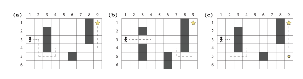
Figure 11: (Color online) Three setups of the grid-world task. Left: The basic grid-world as presented in Ref. sutton1990integrated ; Middle: Some of the walls are positioned differently; Right: The basic grid-world with a distracting small reward $\lambda_{\min}$ placed 12 steps from the agent. In all three setups a large reward of $\lambda_{\max}$ awaits the agent in 14 steps.

terms of steps per reward as a function of trials. In all cases the optimal performance is 14 steps per one reward. In the last phase, a greedy agent would reach the small reward of $\lambda_{\min}=\frac{1}{3}$ in 12 steps, thus resulting with 36 steps per unit of reward. It is seen that the meta-learning agent performs optimally in all phases, except of the last phase, where the performance is only suboptimal with an average of about $16$ steps per unit reward (instead of $14$). This flexibility through all phases is achieved due to the adjustments of the $\gamma$ parameter, whose progress over time is shown in Fig. 12 (b) in solid blue. Similar to the $n$-ship game, we assume that the $\gamma$-network has already learned that the environment uses the “straightforward” logic, by setting the $h$-value ratio of $10^{5}$ to 1 for choosing rule I. The PS agent with the same $\gamma$-network, but without updated $\eta$-network, performs similarly in the first two phases (Fig. 12 (a) in dashed red) in terms of finding eventually an optimal path. This is to be expected because for finding an optimal path it is only necessary that $0<\eta<1$. It is seen, however, that this agent learns much slower than the full meta-learning agent, so that hundreds of thousands more steps are required on average to find an optimal path. This is also reflected in the behavior of the $\gamma$ parameter: with a random $\eta$ value, the $\gamma$ parameter goes to zero much slower, as shown in Fig. 12 (b).

The importance of the $\eta$ parameter is however better demonstrated in the third phase, where the difference between the achieved performance of the agent with and without $\eta$-learning is very significant. In particular, the PS agent with a random $\eta$ converges to the greedy strategy and gets a unit of reward every $36$ steps (Fig. 12 (a) in dashed red). The reason is that optimal performance (a unit of a reward every $14$ steps) can only be achieved by setting the $\eta$ parameter to a value from a certain, limited, range, which we analyze next.

The range of optimal $\eta$ values can be obtained by focusing on the (4, 9) location in the grid-world (see Fig. 11 (c)). In this location, the agent has two possible actions that lead faster to the large and small rewards, namely up and down, respectively. Because these two actions result with a faster reward, edges corresponding to these actions are enhanced stronger than for the other actions. This enhancement is gained by adding the increments $g^{(t)}(c_{i},c_{j})\lambda$ to the $h$-values at the end of each game, as one can see from the update rule in Eq. (3). If the PS agent follows the greedy strategy, then this increment is equal to $\lambda_{\min}=1/3$ and is added to the edge corresponding to the action “down”. For the optimal strategy the increment is $\lambda_{\max}(1-\eta)^{2}=(1-\eta)^{2}$ (since $\lambda_{\max}=1$), because the large reward occurs two decisions away from the current position and the $g$-value is damped from the value of $1$ to the value of $(1-\eta)^{2}$. The optimal strategy will prevail only if the increment in each game is larger than for the greedy strategy. This is the only case when $0<\eta<1-\sqrt{1/3}<0.43$. Most of the actions in the $\eta$-network of the PS agent have values larger than $0.43$, therefore the agent with random $\eta$ actions converges to the greedy strategy and does not get the best possible reward. The PS agent with meta-learning is able to learn to use the $\eta$ parameter from the optimal range, and as shown in Fig. 12 (c) the agent indeed mostly uses the values of $\eta=0.1$ and $0.2$.

VI Summary and Discussion

We have developed a meta-learning machinery that allows the PS agent to dynamically adjust its own meta-parameters. This was shown to be desirable by demonstrating that, like in other AI schemes, no unique choice of the model’s learning parameters can account for all possible tasks, as optimal values for the meta-parameters vary from one task environment to another. We emphasize that the presented meta-learning component is based on the same design as the basic PS, using random walk on clip-networks as the central information processing step. It is therefore naturally integrated into the PS learning framework, preserving the model’s stochastic nature, along with its simplicity.

The basic PS has two principal meta-parameters: the damping parameter $\gamma$ and the glow parameter $\eta$. For each meta-parameter we have assigned a meta-learning clip-network, whose actions control the parameter’s value. Each meta-level network is activated every fixed number of interactions with the environment. This time

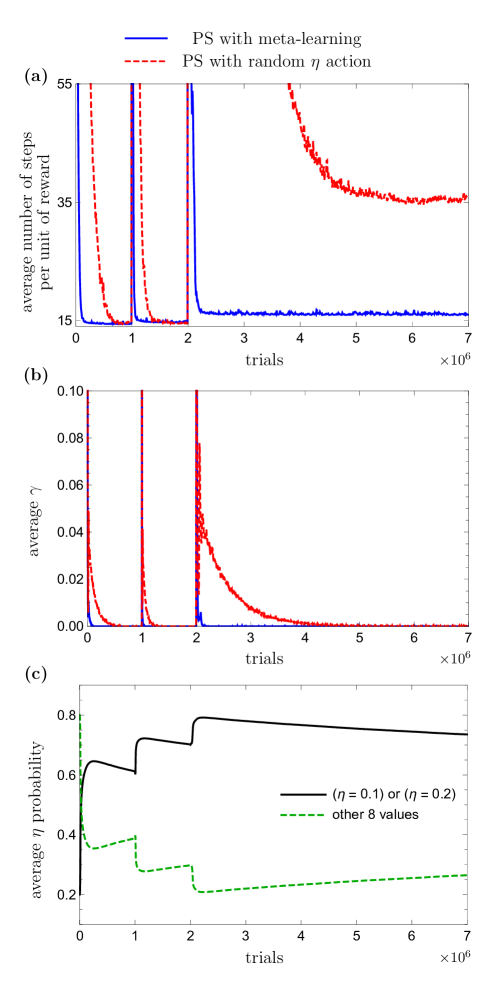
Figure 12: (Color online) Grid-world task: Two types of PS agents are depicted: with full meta-learning capability (in solid blue), and with adjusted $\gamma$ value but with $\eta$ value that is chosen randomly from the ECM_η network (in dashed red). Top: The performances of the two different agents are shown as a function of trials in terms of average number of steps per unit reward; Middle: The average $\gamma$ values of the two different kinds of agents are shown as a function of trials; Bottom: For the meta-learning PS agent the probability to choose $\eta=0.1$ or $\eta=0.2$ and the probability to choose either of the other 8 $\eta$-actions are plotted as a function of trials; The first two phases of the game last $10^{6}$ trials, whereas the last phase lasts $5\times 10^{6}$ trials. These phases correspond to three different kinds of grid-worlds shown in Fig. 11. The simulations were done by averaging over $10^{4}$ agents.

window allows the agent to gather statistics about its performance, so as to monitor its recent success rates and thereby to evaluate the setting of the corresponding parameters. When the agent’s success increases, the previous action of the meta-level network is rewarded positively, otherwise, when the performance deteriorates, a negative reward is assigned (no reward is assigned when there is no change in the agent’s success). As a result, the probability that the random walk on the meta-level network hits more favorable action clips increases with time and the meta-level network essentially learns how to properly adjust the corresponding parameter in the current environment.

The meta-learning process occurs on a much larger time-scale compared to the base-level network learning time scale. This is necessary as meta-level learning requires statistical knowledge of the agent’s performance, which is directly controlled by the base-level network, whose learning time is linear with the state space of the task, represented by the number of percepts and actions in the base-level network.

In meta-level learning we have distinguished between adaptation through learning, which exploits the entire individual history of the agent to update the value of the meta-parameter, and reflexive adaptation, which updates the meta-parameter using only recent, localized information of the agent’s performance. We saw that the glow parameter can be well adjusted with a full learning network that is only via adaptation through learning, whereas for the damping parameter, it is more sensible to combine the two kinds of adaptations.

The presented meta-learning scheme was examined in three different environmental scenarios, each of which requires a different set of meta-parameters for optimal performance. Specifically, we have considered the “invasion game”, where there are no temporal correlations between actions and rewards (implying that the optimal glow value is $\eta_{\text{opt}}=1$), the “$n$-ship game” where temporal correlations do exist and $\eta_{\text{opt}}$ depends on $n$, and finally the “grid-world”, a real-world scenario with delayed rewards, for which it is sufficient that $\eta_{\text{opt}}\neq 1$ in the basic setup, but requires that $\eta_{\text{opt}}<<1$ in the more advanced setup, where the agent can be distracted by a small reward.

In all scenarios, the environment furthermore suddenly changes, thus requiring the agent to also adjust its forgetting parameter $\gamma$. Overall, situating an agent in such changing environments enforces it to repeatedly and dynamically revise its internal settings. The meta-learning PS agent was shown to cope well in all scenarios, reaching success probabilities that approach near-optimal or optimal values.

For comparison, we checked how a PS agent with fixed set of random meta-parameters would handle these scenarios, and observed that such an agent would perform significantly worse. This is not surprising, as most of the possible meta-parameter values (especially those of the $\gamma$ parameter) are harmful for the agent. Therefore, for a more challenging comparison, we checked the performance of an agent that adapts its forgetting parameter $\gamma$ in exactly the same way as the meta-learning agent, but chooses its glow parameter $\eta$ randomly, out of the same set of actions available in the $\eta$-network we used. Such an intermediate agent performed better than the basic PS agent with random choice of meta-parameters, but substantially worse than the full meta-learning agent. This demonstrates the importance of adjusting both $\gamma$ and $\eta$ in a proper way. In particular, it shows that the learning of the $\eta$-network plays a crucial role.

Importantly, throughout the paper, we used the same set of choices for the meta-learning scheme. In particular, we used the same meta-level networks ECM_γ (including the reflexive rules of the $\gamma$-parameter adaptation) and ECM_η, and the same time windows $\tau_{\gamma}$ and $\tau_{\eta}$. This indicates that the suggested meta-learning scheme is robust, as it requires no further adjustment of additional parameters by an external party, for all the cases we have considered.

References

- (1) Russell, S. J. & Norvig, P. Artificial Intelligence - A Modern Approach, chap. 4 (Pearson Education, New Jersey, 2003).
- (2) Brazdil, P., Giraud-Carrier, C., Soares, C. & Vilalta, R. Metalearning: Applications to Data Mining (Springer, 2009).
- (3) Wolpert, D. & Macready, W. No free lunch theorems for optimization. IEEE Transactions on Evolutionary Computation 1, 67–82 (1997).
- (4) Wilson, S. W. Classifier fitness based on accuracy. Evolutionary computation 3, 149–175 (1995).
- (5) Schaul, T. & Schmidhuber, J. Metalearning. Scholarpedia 5, 4650 (2010).
- (6) Giraudo-Carrier, C., Vilalta, R. & Brazdil, P. Introduction to the special issue on meta-learning. Machine Learning 54, 187–193 (2004).
- (7) Thrun, S. & Pratt, L. (eds.) Learning to learn (Springer Science & Business Media, 1998).
- (8) Duch, W. & Grudziński, K. Meta-learning via search combined with parameter optimization. In Kłopotek, M., Wierzchoń, S. & Michalewicz, M. (eds.) Intelligent Information Systems 2002, vol. 17 of Advances in Soft Computing, 13–22 (Physica-Verlag HD, 2002).
- (9) Brazdil, P., Soares, C. & da Costa, J. Ranking learning algorithms: Using IBL and meta-learning on accuracy and time results. Machine Learning 50, 251–277 (2003).
- (10) Zhao, P. & Yu, B. On model selection consistency of lasso. Journal of Machine Learning Research 7, 2541–2563 (2006).
- (11) Adankon, M. M. & Cheriet, M. Model selection for the LS-SVM. Application to handwriting recognition. Pattern Recognition 42, 3264–3270 (2009).
- (12) Abdulrahman, S. M., Brazdil, P., van Rijn, J. N. & Vanschoren, J. Algorithm selection via meta-learning and sample-based active testing. In Proceedings of the Meta-learning and algorithm selection workshop at ECMLPKDD 2015, 55–66 (2015).
- (13) Todorovski, L. & Džeroski, S. Combining classifiers with meta decision trees. Machine Learning 50, 223–249 (2003).
- (14) Ishii, S., Yoshida, W. & Yoshimoto, J. Control of exploitation–exploration meta-parameter in reinforcement learning. Neural Networks 15, 665 – 687 (2002).
- (15) Schweighofer, N. & Doya, D. Meta-learning in reinforcement learning. Neural Networks 16, 5–9 (2003).
- (16) Eriksson, A., Capi, G. & Doya, K. Evolution of meta-parameters in reinforcement learning algorithm. In Proceedings of the IEEE/RSJ International Conference on Intelligent Robots and Systems 2003.
- (17) Kobayashi, K., Mizoue, H., Kuremoto, T. & Obayashi, M. A meta-learning method based on temporal difference error. In Leung, C., Lee, M. & Chan, J. (eds.) Neural Information Processing, vol. 5863 of Lecture Notes in Computer Science, 530–537 (Springer Berlin Heidelberg, 2009).
- (18) Tokic, M., Schwenker, F. & Palm, G. Meta-learning of exploration and exploitation parameters with replacing eligibility traces. In Zhou, Z.-H. & Schwenker, F. (eds.) Partially Supervised Learning, vol. 8183 of Lecture Notes in Computer Science, 68–79 (Springer Berlin Heidelberg, 2013).
- (19) Bengio, Y. Gradient-based optimization of hyperparameters. Neural computation 12, 1889–1900 (2000).
- (20) Bardenet, R. & Kégl, B. Surrogating the surrogate: accelerating gaussian-process-based global optimization with a mixture cross-entropy algorithm. In Proceedings of the 27th International Conference on Machine Learning, 55–62 (2010).
- (21) Bergstra, J. & Bengio, Y. Random search for hyper-parameter optimization. Journal of Machine Learning Research 13, 281–305 (2012).
- (22) Reif, M., Shafait, F. & Dengel, A. Meta-learning for evolutionary parameter optimization of classifiers. Machine learning 87, 357–380 (2012).
- (23) Thornton, C., Hutter, F., Hoos, H. H. & Leyton-Brown, K. Auto-weka: Combined selection and hyperparameter optimization of classification algorithms. In Proceedings of the 19th ACM SIGKDD International Conference on Knowledge Discovery and Data Mining, 847–855 (ACM, 2013).
- (24) Smith, M., Mitchell, L., Giraud-Carrier, C. & Martinez, T. Recommending learning algorithms and their associated hyperparameters. In Proceedings of the Meta-learning and algorithm selection workshop at ECAI 2014, 39–40 (2014).
- (25) Feurer, M., Springenberg, T. & Hutter, F. Initializing Bayesian hyperparameter optimization via meta-learning. In Proceedings of the 29th AAAI Conference on Artificial Intelligence, 1128–1135 (2015).
- (26) Sutton, R. S. & Barto, A. G. Reinforcement learning: An introduction (MIT Press, Cambridge Massachusetts, 1998).
- (27) Achbany, Y., Fouss, F., Yen, L., Pirotte, A. & Saerens, M. Tuning continual exploration in reinforcement learning: An optimality property of the boltzmann strategy. Neurocomputing 71, 2507 – 2520 (2008). Artificial Neural Networks (ICANN 2006) / Engineering of Intelligent Systems (ICEIS 2006).
- (28) Schmidhuber, J. Completely self-referential optimal reinforcement learners. In Artificial Neural Networks: Formal Models and Their Applications, vol. 3697 of Lecture Notes in Computer Science, 223–233 (Springer Berlin Heidelberg, 2005).
- (29) Briegel, H. J. & De las Cuevas, G. Projective simulation for artificial intelligence. Scientific Reports 2, 400 (2012).
- (30) Mautner, J., Makmal, A., Manzano, D., Tiersch, M. & Briegel, H. J. Projective simulation for classical learning agents: a comprehensive investigation. New Generation Computing 33, 69–114 (2015).
- (31) Melnikov, A. A., Makmal, A. & Briegel, H. J. Projective simulation applied to the grid-world and the mountain-car problem. Artificial Intelligence Research 3 (3), 24–34 (2014). arXiv:1405.5459.
- (32) Bjerland, Ø. F. Projective Simulation compared to reinforcement learning. Master’s thesis, University of Bergen, Norway (2015).
- (33) Melnikov, A. A., Makmal, A., Dunjko, V. & Briegel, H. J. Projective simulation with generalization. Preprint, arXiv:1504.02247 [cs.AI] (2015).
- (34) Pfeiffer, R. & Scheier, C. Understanding intelligence (MIT Press, Cambridge Massachusetts, 1999).
- (35) Motwani, R. & Raghavan, P. Randomized Algorithms, chap. 6 (Cambridge University Press, New York, NY, USA, 1995).
- (36) Feynman, R. P. & Hibbs, A. R. Quantum mechanics and path integrals. International series in pure and applied physics (McGraw-Hill, New York, 1965).
- (37) Aharonov, Y., Davidovich, L. & Zagury, N. Quantum random walks. Physical Review A 48, 1687–1690 (1993).
- (38) Aharonov, D., Ambainis, A., Kempe, J. & Vazirani, U. Quantum walks on graphs. In Proceedings of the 33rd Annual ACM Symposium on Theory of Computing, STOC ’01, 50–59 (ACM, New York, 2001).
- (39) Childs, A. M. et al. Exponential algorithmic speedup by a quantum walk. In Proceedings of the 35th Annual ACM Symposium on Theory of Computing, STOC ’03, 59–68 (ACM, New York, 2003).
- (40) Kempe, J. Discrete quantum walks hit exponentially faster. Probability Theory and Related Fields 133, 215–235 (2005).
- (41) Krovi, H., Magniez, F., Ozols, M. & Roland, J. Quantum walks can find a marked element on any graph. Algorithmica 1–57 (2015).
- (42) Paparo, G. D., Dunjko, V., Makmal, A., Martin-Delgado, M. A. & Briegel, H. J. Quantum speed-up for active learning agents. Physical Review X 4, 031002 (2014).
- (43) Dunjko, V., Friis, N. & Briegel, H. J. Quantum-enhanced deliberation of learning agents using trapped ions. New Journal of Physics 17, 023006 (2015).
- (44) Friis, N., Melnikov, A. A., Kirchmair, G. & Briegel, H. J. Coherent controlization using superconducting qubits. Scientific Reports 5, 18036 (2015).
- (45) Anderson, M. L. & Oats, T. A review of recent research in metareasoning and metalearning. AI Magazine 28, 7–16 (2007).
- (46) Rummery, G. A. & Niranjan, M. On-line Q-learning using connectionist systems. Tech. Rep., University of Cambridge (1994).
- (47) Wang, C.-C., Kulkarni, S. R. & Poor, H. V. Bandit problems with side observations. IEEE Transactions on Automatic Control 50, 338–355 (2005).
- (48) Sutton, R. S. Integrated architectures for learning, planning, and reacting based on approximating dynamic programming. In Proceedings of the 7th International Conference on Machine Learning, 216–224 (1990).