Justification of the Nonlinear Schrödinger approximation for a quasilinear Klein-Gordon equation

Abstract.

We consider a nonlinear Klein-Gordon equation with a quasilinear quadratic term. The Nonlinear Schrödinger (NLS) equation can be derived as a formal approximation equation describing the evolution of the envelopes of slowly modulated spatially and temporarily oscillating wave packet-like solutions to the quasilinear Klein-Gordon equation. It is the purpose of this paper to present a method which allows one to prove error estimates in Sobolev norms between exact solutions of the quasilinear Klein-Gordon equation and the formal approximation obtained via the NLS equation. The paper contains the first validity proof of the NLS approximation of a nonlinear hyperbolic equation with a quasilinear quadratic term by error estimates in Sobolev spaces. We expect that the method developed in the present paper will allow an answer to the relevant question of the validity of the NLS approximation for other quasilinear hyperbolic systems.

1. Introduction and Result

The Nonlinear Schrödinger (NLS) equation plays an important role in describing approximately slow modulations in time and space of an underlying spatially and temporarily oscillating wave packet in a more complicated hyperbolic system, such as Maxwell’s equations for modeling nonlinear optics or the equations describing surface water waves, see, for example, [1]. In this paper, we study the NLS approximation of the quasilinear Klein-Gordon equation

(1) $$\partial_{t}^{2}u=\partial_{x}^{2}u-u+\partial_{x}^{2}(u^{2})\,,$$

with $x,t\in\mathbb{R}$, and $u(x,t)\in\mathbb{R}$. We make the ansatz $u=\varepsilon\Psi_{NLS}+\mathcal{O}(\varepsilon^{2})$, with

(2) $$\varepsilon\Psi_{NLS}(x,t)=\varepsilon A(\varepsilon(x-c_{g}t),\varepsilon^{2}t)e^{i(k_{0}x-\omega_{0}t)}+\mathrm{c.c.}\,.$$

Here $0<\varepsilon\ll 1$ is a small perturbation parameter, $\omega_{0}>0$ the basic temporal wave number associated to the basic spatial wave number $k_{0}>0$ of the underlying carrier wave $e^{i(k_{0}x-\omega_{0}t)}$, $c_{g}$ the group velocity, $A$ the complex-valued amplitude, and c.c. the complex conjugate. With the help of (2) we describe slow spatial and temporal modulations of the underlying carrier wave. Inserting the above ansatz into (1) we find that $A$ satisfies at leading order in $\varepsilon$ the NLS equation

(3) $$\partial_{T}A=i\nu_{1}\partial_{X}^{2}A+i\nu_{2}A|A|^{2}\,,$$

where $X=\varepsilon(x-c_{g}t)$, $T=\varepsilon^{2}t$, and $\nu_{j}=\nu_{j}(k_{0})\in\mathbb{R}$. $T$ is the slow time scale and $X$ is the slow spatial scale, that means, the time scale of the modulations is $\mathcal{O}({1/\varepsilon^{2}})$ and the spatial scale of the modulations is $\mathcal{O}({1/\varepsilon})$. See Figure 1. The basic spatial wave number $k=k_{0}$ and the basic temporal wave number $\omega=\omega_{0}$ are related via the linear dispersion relation of the quasilinear Klein-Gordon equation (1), namely

(4) $$\omega^{2}(k)-(1+k^{2})=0\,,$$

where we choose the branch of solutions

(5) $$\omega(k):=\ {\rm sign}(k)\sqrt{1+k^{2}}\,.$$

Then the group velocity $c_{g}$ of the wave packet is given by $c_{g}=\partial_{k}\omega|_{k=k_{0}}$. Our ansatz leads to waves moving to the right. To obtain waves moving to the left, $-\omega_{0}$ and $c_{g}$ have to be replaced by $\omega_{0}$ and $-c_{g}$.

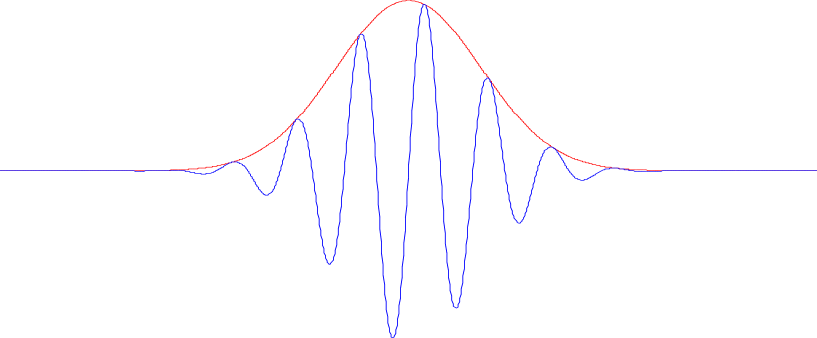
$c_{\mathrm{g}}$

$c_{\mathrm{p}}$

$\varepsilon$

$1/\varepsilon$

Figure 1. The envelope (advancing with the group velocity $c_{g}$) of the oscillating wave packet (advancing with the phase velocity $c_{p}=\omega_{0}/k_{0}$) is described by the amplitude $A$ which solves the NLS equation (3).

It is the goal of the present paper to prove

Theorem 1.1.

Fix $s_{A}\geq 6$. Then for all $k_{0}>0$ and for all $C_{1},T_{0}>0$ there exist $C_{2}>0$, $\varepsilon_{0}>0$ such that for all solutions $A\in C([0,T_{0}],H^{s_{A}}(\mathbb{R},\mathbb{C}))$ of the NLS equation (3) with

$$\sup_{T\in[0,T_{0}]}\|A(\cdot,T)\|_{H^{s_{A}}(\mathbb{R},\mathbb{C})}\leq C_{1}$$

the following holds. For all $\varepsilon\in(0,\varepsilon_{0})$ there are solutions

$$u\in C([0,T_{0}/\varepsilon^{2}],H^{s_{A}}(\mathbb{R},\mathbb{R}))$$

of the quasilinear Klein-Gordon equation (1) which satisfy

$$\sup_{t\in[0,T_{0}/\varepsilon^{2}]}\|u(\cdot,t)-\varepsilon\Psi_{NLS}(\cdot,t)\|_{H^{s_{A}}(\mathbb{R},\mathbb{R})}\leq C_{2}\varepsilon^{3/2}.$$

The error of order $\mathcal{O}(\varepsilon^{3/2})$ is small compared with the solution $u$ and the approximation $\varepsilon\Psi_{NLS}$, which are both of order $\mathcal{O}(\varepsilon)$ in $L^{\infty}$ such that the dynamics of the NLS equation can be found in the quasilinear Klein-Gordon equation (1), too. The NLS equation is a completely integrable Hamiltonian system, which can be solved explicitly with the help of some inverse scattering scheme, see, for example, [1].

It should be noted that the smoothness in our error bound is equal to the assumed smoothness of the amplitude. This can be achieved by using a modified approximation which has compact support in Fourier space but differs only slightly from $\varepsilon\Psi_{NLS}$. Such an approximation can be constructed because the Fourier transform of $\varepsilon\Psi_{NLS}$ is sufficiently strongly concentrated around the wave numbers $\pm k_{0}$.

Like in many other proofs of error estimates in the literature we will assume in our proof of Theorem 1.1 that $s_{A}$ is an integer in order to simplify the analysis by using Leibniz’s rule, but our proof can be generalized to be valid for all $s_{A}\geq 6$.

We remark that such an approximation theorem like Theorem 1.1 should not be taken for granted. There are various counterexamples, where approximation equations derived by reasonable formal arguments make wrong predictions about the dynamics of the original systems, see, for example, [16, 19]. For an introduction into theory and applications of the NLS approximation we refer to [17].

In order to explain our method to prove Theorem 1.1 and the relevance of this method we consider the more general abstract evolutionary problem

(6) $$\partial_{t}V=\Lambda V+B(V,V)\,,$$

with $V=V(x,t)\in\mathbb{R}^{2}$, $x,t\in\mathbb{R}$, $\Lambda$ a linear operator whose symbol is a diagonal matrix of the form

(7) $$\widehat{\Lambda}(k)=\mathrm{diag}\,(-i\lambda(k),\,i\lambda(k))\,,$$

where $k\in\mathbb{R}$ and $\lambda$ is a piecewise smooth real-valued odd function, and $B$ a symmetric bilinear operator. Writing the quasilinear Klein-Gordon equation (1) as a first-order system and diagonalizing the linear part of the resulting system we obtain a special case of (6), where $\lambda=\omega$, with $\omega$ defined by (5).

The NLS equation (3) can be derived as a formal approximation equation with the help of the ansatz $V=\varepsilon\tilde{\Psi}$, where

(12) $$\varepsilon\tilde{\Psi}(x,t)=\; \varepsilon\left(\begin{array}[]{c}\Psi_{NLS}(x,t)\\ 0\\ \end{array}\right)+\varepsilon^{2}\left(\begin{array}[]{c}{\widetilde{A}}_{01}(\varepsilon(x-c_{g}t),\varepsilon^{2}t)\\ {\widetilde{A}}_{02}(\varepsilon(x-c_{g}t),\varepsilon^{2}t)\\ \end{array}\right)$$

(15) $$+\varepsilon^{2}\left(\left(\begin{array}[]{c}{\widetilde{A}}_{21}(\varepsilon(x-c_{g}t),\varepsilon^{2}t)\\ {\widetilde{A}}_{22}(\varepsilon(x-c_{g}t),\varepsilon^{2}t)\\ \end{array}\right)e^{2i(k_{0}x-\omega_{0}t)}+\mathrm{c.c.}\right),$$

with $\Psi_{NLS}$ as in (2), where $\omega_{0}=\lambda(k_{0})$ and $c_{g}=\partial_{k}\lambda(k_{0})$, real-valued functions ${\widetilde{A}}_{01},{\widetilde{A}}_{02}$, and complex-valued functions ${\widetilde{A}}_{21},{\widetilde{A}}_{22}$. Inserting this ansatz into (6) and equating the coefficients in front of the $\varepsilon^{m}e^{ji(k_{0}x-\omega_{0}t)}$ for $m\in\{1,2,3\}$ and $j\in\{0,1,2\}$ to zero yields the NLS equation (3) if $\lambda$ satisfies $\lim\limits_{k\to 0^{\pm}}\lambda(k)\neq 0$ or $\lim\limits_{k\to 0^{\pm}}\partial_{k}\lambda(k)\neq c_{g}$ as well as $\pm\lambda(2k_{0})\neq 2\lambda(k_{0})$, which is true for $\lambda=\omega$.

It is possible to modify $\varepsilon\tilde{\Psi}$ to make it an even more accurate approximation. Indeed, for all $\gamma>0$ there exists a function $\Psi$ such that $\Psi-\tilde{\Psi}\to 0$ for $\varepsilon\to 0$ and

(16) $$\mbox{Res}(\varepsilon\Psi):=-\partial_{t}(\varepsilon\Psi)+\Lambda(\varepsilon\Psi)+B(\varepsilon\Psi,\varepsilon\Psi)=\mathcal{O}(\varepsilon^{\gamma})\,.$$

In order to prove Theorem 1.1 we have to estimate the error

(17) $$\varepsilon^{\beta}R:=V-\varepsilon{\Psi}$$

for all $t\in[0,T_{0}/\varepsilon^{2}]$ to be of order $\mathcal{O}(\varepsilon^{\beta})$ for a $\beta>1$, that means, we have to prove that $R$ is of order $\mathcal{O}(1)$ for all $t\in[0,T_{0}/\varepsilon^{2}]$. The error $R$ satisfies the equation

(18) $$\partial_{t}R=\Lambda R+2\varepsilon^{\alpha}B({\Psi},R)+\varepsilon^{\beta}B(R,R)+\varepsilon^{-\beta}\mbox{Res}(\varepsilon{\Psi})\,,$$

with $\alpha=1$.

Since our linear operator $\Lambda$ generates a uniformly bounded strongly continuous semigroup, we would be done if we had a) $\alpha\geq 2$, b) $\beta>2$, and c) $\varepsilon^{-\beta}{\rm Res}(\varepsilon{\Psi})=\mathcal{O}(\varepsilon^{2})$. The result then would follow by a rescaling of time, $T=\varepsilon^{2}t$, and an application of Gronwall’s inequality, see, for example, [12]. However, we have $\alpha=1$. We can still make $\gamma$ in (16) arbitrary large by constructing our approximate solution $\varepsilon\Psi$ as described below, and in particular, strictly bigger than $4$. Consequently, we can choose $\beta>2$ and so the points b) and c) are satisfied easily. Hence, the difficulty is to control the quadratic term $2\varepsilon B({\Psi},R)$.

Semilinear quadratic terms can be eliminated with the help of a so-called normal-form transform

(19) $$\tilde{R}:=R+\varepsilon N({\Psi},R)\,,$$

where $N$ is an appropriately constructed bilinear mapping, if the so-called non-resonance condition

(20) $$\inf_{k\in\mathbb{R},\atop j_{1},j_{2}\in\{\pm 1\}}\,|{-j_{1}\lambda(k)-\lambda(k_{0})+j_{2}\lambda(k-k_{0})}|\geq C>0$$

is satisfied. This normal-form transform is invertible and the new error function $\tilde{R}$ satisfies an evolution equation of the form

(21) $$\partial_{t}\tilde{R}=\Lambda\tilde{R}+\varepsilon^{2}g({\Psi},\tilde{R})+\varepsilon^{-\beta}\mbox{Res}(\varepsilon{\Psi})\,,$$

where $g({\Psi},\tilde{R})$ is a semilinear term of order $\mathcal{O}(1)$. Therefore, to this equation, Gronwall’s inequality can be applied to bound $\tilde{R}$ and hence $R$ for all $t\in[0,T_{0}/\varepsilon^{2}]$.

The strategy of using normal-form transforms to eliminate semilinear quadratic terms in hyperbolic systems was introduced in [23]. In the context of justifying NLS approximations, it was first applied in [11] and was further developed in [14, 15], where also first attempts were made to weaken the non-resonance condition (20). Proving the validity of 2D NLS approximations with the help of a normal-form transform was addressed in [5].

However, in the case of equation (1) the quadratic term $2\varepsilon B({\Psi},R)$ is quasilinear and loses one derivative, that means, $R\mapsto 2\varepsilon B({\Psi},R)$ maps $H^{m+1}(\mathbb{R},\mathbb{C})$ into $H^{m}(\mathbb{R},\mathbb{C})$ or $C^{n+1}(\mathbb{R},\mathbb{C})$ into $C^{n}(\mathbb{R},\mathbb{C})$. Since the non-resonance condition (20) is satisfied for $\lambda=\omega$, it is still possible to construct a normal-form transform of the form (19) to eliminate this term. But the normal-form transform also loses one derivative. At least, the term $2\varepsilon B({\Psi},R)$ being generated by equation (1) has a structure that nevertheless allows one to invert the normal-form transform. Hence, the new error function $\tilde{R}$ still satisfies an evolution equation of the form (21), but the loss of one derivative caused by the normal-form transform implies that the term $g({\Psi},\tilde{R})$ loses even two derivatives.

Consequently, the variation of constants formula and Gronwall’s inequality cannot be applied to bound $\tilde{R}$ - in this situation not because of missing powers of $\varepsilon$ but due to regularity problems, since the semigroup generated by $\Lambda$ is not smoothing. For the same reasons it does not work either to bound $\tilde{R}$ by deriving energy inequalities for $\tilde{R}$ and applying Gronwall’s inequality to them.

Hence, the validity of the NLS approximation for hyperbolic systems with quasilinear quadratic terms is a highly nontrivial problem, which has been remained unsolved in general for more than four decades. Only for some examples of quasilinear systems the NLS approximation has been justified so far. All these examples avoid the major difficulty captured by equation (1).

The first and very general NLS approximation theorem for quasilinear dispersive wave systems was proven in [11]. However, the occurrence of quasilinear quadratic terms was excluded explicitly. Another example are dispersive wave systems where the right-hand sides lose only half a derivative. The 2D water wave problem without surface tension and finite depth in Lagrangian coordinates falls into this class. In this case the elimination of the quadratic terms is possible with the help of normal-form transforms. The right-hand sides of the transformed systems then lose one derivative and can be handled with the help of the Cauchy-Kowalevskaya theorem [22, 7]. Furthermore, the NLS approximation was justified for the 2D and 3D water wave problem without surface tension and infinite depth [25, 24] by finding a different transform adapted to the special structure of that problem. Similarly, for the quasilinear Korteweg-de Vries equation the result can be obtained by simply applying a Miura transform [18]. In [2], the NLS approximation of time oscillatory long waves for equations with quasilinear quadratic terms was proven for analytic data without using a normal-form transform. Moreover, another approach to address the problem of the validity of the NLS approximation can be found in [13]. Finally, some numerical evidence that the NLS approximation is also valid for quasilinear equations like equation (1) was given in [3].

The present paper contains the first validity proof of the NLS approximation of a nonlinear hyperbolic equation with a quasilinear quadratic term in Sobolev spaces. We expect that the method developed here will allow an answer to the relevant question of the validity of the NLS approximation for many other quasilinear hyperbolic systems. Our method of proof is as follows.

Instead of performing the normal-form transform (19) we only use the term $\varepsilon N(\Psi,R)$ to define the energy

(22) $$\mathcal{E}_{s}=\sum_{\ell=0}^{s}\Big{(}\frac{1}{2}\|\partial_{x}^{\ell}R\|_{L^{2}}^{2}+\varepsilon\int_{\mathbb{R}}\partial_{x}^{\ell}R\bullet\partial_{x}^{\ell}N(\Psi,R)\,dx\Big{)}\,,$$

where $s=s_{A}\geq 6$. Since $\|\tilde{R}\|_{H^{s}}^{2}$ differs from $\mathcal{E}_{s}$ only by terms of order $\mathcal{O}(\varepsilon^{2})$, the evolution equations of $\mathcal{E}_{s}$ and $\|\tilde{R}\|_{H^{s}}^{2}$ share the property that their right-hand sides are of order $\mathcal{O}(\varepsilon^{2})$.

This strategy was already used in [4] as an ingredient to simplify the proof of error estimates compared with the alternative proofs in [20, 21]. To overcome regularity problems caused by quasilinear quadratic terms, this strategy was first used in [9] and was further developed in [8, 10] to apply it to the water wave problem with infinite depth. In these three papers, structural properties of the Hilbert transform help to construct and estimate the energy.

In the case of equation (1) we can show that $N(\Psi,R)$ can be split into a term of the form $\mathrm{diag}\,(f_{1}(\Psi),\,f_{2}(\Psi))\,\partial_{x}R$ and terms which do not lose regularity such that partial integration yields the equivalence of $\sqrt{\mathcal{E}_{s}}$ and $\|R\|_{H^{s}}$ for sufficiently small $\varepsilon$. Consequently, the right-hand side of the evolution equation of $\mathcal{E}_{s}$ can be written as a sum of integral terms containing at most one factor $\partial_{x}^{s+1}R$ and not two.

Therefore, the structure of $\Lambda$ and the properties of $\omega$ allow us to construct a modified energy

(23) $$\tilde{\mathcal{E}_{s}}=\mathcal{E}_{s}+\varepsilon^{2}h\,,$$

where $h=\mathcal{O}(\|R\|_{H^{s}}^{2})$ as long as $\|R\|_{H^{s}}=\mathcal{O}(1)$ and $\varepsilon^{2}\partial_{t}h$ eliminates all the integral terms on the right-hand side of the evolution equation of $\mathcal{E}_{s}$ with a factor $\partial_{x}^{s+1}R$. Consequently, we obtain

(24) $$\partial_{t}\tilde{\mathcal{E}_{s}}\lesssim\varepsilon^{2}(\tilde{\mathcal{E}_{s}}+1)$$

as long as $\|R\|_{H^{s}}=\mathcal{O}(1)$ such that Gronwall’s inequality yields the $\mathcal{O}(1)$-boundedness of $\tilde{\mathcal{E}_{s}}$ and hence of $R$ for all $t\in[0,T_{0}/\varepsilon^{2}]$.

We finish the discussion of our method of proof with a comment on the chosen regularity of the quadratic nonlinearity. The term $\partial_{x}^{2}(u^{2})$ is the least regular quadratic term which can be added to the linear part of the right-hand side of equation (1) so that the method developed in the present paper allows us to construct an energy $\tilde{\mathcal{E}_{s}}$ satisfying (23)-(24) as long as $\|R\|_{H^{s}}=\mathcal{O}(1)$. It is a question of ongoing research if this method can be generalized to be applicable to less regular nonlinearities.

The plan of the paper is as follows. In Section 2 we rewrite the quasilinear Klein-Gordon equation (1) to make it a special case of the evolutionary system (6) and derive the NLS approximation. In Section 3 we present the error equations, construct our energy and perform the error estimates to prove Theorem 1.1.

In a forthcoming paper, we intend to combine the methods of the present paper with the methods from [4, 6] to generalize the approximation theorem for the NLS approximation from [6] to the case of the water wave problem with surface tension.

Notation. We denote the Fourier transform of a function $u\in L^{2}(\mathbb{R},\mathbb{K})$, with $\mathbb{K}=\mathbb{R}$ or $\mathbb{K}=\mathbb{C}$ by

$$\hat{u}(k)=\frac{1}{2\pi}\int_{\mathbb{R}}u(x)e^{-ikx}dx.$$

Let $H^{s}(\mathbb{R},\mathbb{K})$ be the space of functions mapping from $\mathbb{R}$ into $\mathbb{K}$ for which the norm

$$\|u\|_{H^{s}(\mathbb{R},\mathbb{K})}=\left(\int_{\mathbb{R}}|\hat{u}(k)|^{2}(1+|k|^{2})^{s}dk\right)^{1/2}$$

is finite. We also write $L^{2}$ and $H^{s}$ instead of $L^{2}(\mathbb{R},\mathbb{R})$ and $H^{s}(\mathbb{R},\mathbb{R})$. Moreover, we use the space $L^{p}(m)(\mathbb{R},\mathbb{K})$ defined by $u\in L^{p}(m)(\mathbb{R},\mathbb{K})\Leftrightarrow u\sigma^{m}\in L^{p}(\mathbb{R},\mathbb{K})$, where $\sigma(x)=(1+x^{2})^{1/2}$.

Furthermore, we write $A\lesssim B$, if $A\leq CB$ for a constant $C>0$, and $A=\mathcal{O}(B)$, if $|A|\lesssim B$.

2. The Derivation of the NLS Approximation

We rewrite the quasilinear Klein-Gordon equation

$$\partial_{t}^{2}u=\partial_{x}^{2}u-u+\partial_{x}^{2}(u^{2})$$

as a first-order system

(25) $$\partial_{t}u =\sqrt{1-\partial_{x}^{2}}\,Hv\,,$$

(26) $$\partial_{t}v =\sqrt{1-\partial_{x}^{2}}\,Hu-\partial_{x}^{2}(1-\partial_{x}^{2})^{-1/2}H(u^{2})\,,$$

where $H$ denotes the Hilbert transform. In Fourier space we have

(27) $$\partial_{t}\widehat{u}(k,t) =-i\omega(k)\widehat{v}(k,t)\,,$$

(28) $$\partial_{t}\widehat{v}(k,t) =-i\omega(k)\widehat{u}(k,t)-i\rho(k)(\widehat{u}\ast\widehat{u})(k,t)\,,$$

where

(29) $$\omega(k)=\mathrm{sign}(k)\sqrt{1+k^{2}}$$

and

(30) $$\rho(k)=\mathrm{sign}(k)\frac{k^{2}}{\sqrt{1+k^{2}}}\,.$$

We diagonalize this system by

(31) $$\left(\begin{array}[]{c}\widehat{u}\\ \widehat{v}\end{array}\right)=\left(\begin{array}[]{cc}1&1\\ 1&-1\end{array}\right)\left(\begin{array}[]{c}\widehat{u}_{-1}\\ \widehat{u}_{1}\end{array}\right).$$

Then we obtain

(32) $$\left(\begin{array}[]{c}\widehat{u}_{-1}\\ \widehat{u}_{1}\end{array}\right)=\frac{1}{2}\left(\begin{array}[]{cc}1&1\\ 1&-1\end{array}\right)\left(\begin{array}[]{c}\widehat{u}\\ \widehat{v}\end{array}\right)$$

and

(33) $$\partial_{t}\widehat{u}_{-1}(k,t) =-i\omega(k)\widehat{u}_{-1}(k,t)-\frac{1}{2}i\rho(k)(\widehat{u}_{-1}+\widehat{u}_{1})^{\ast 2}(k,t)\,,$$

(34) $$\partial_{t}\widehat{u}_{1}(k,t) =i\omega(k)\widehat{u}_{1}(k,t)+\frac{1}{2}i\rho(k)(\widehat{u}_{-1}+\widehat{u}_{1})^{\ast 2}(k,t)\,.$$

In order to derive the NLS equation as an approximation equation for system (33)-(34) we make the ansatz

(35) $$\left(\begin{array}[]{c}{u}_{-1}\\ {u}_{1}\end{array}\right)=\varepsilon\widetilde{\Psi}=\varepsilon{\widetilde{\Psi}}_{1}+\varepsilon{\widetilde{\Psi}}_{-1}+\varepsilon^{2}{\widetilde{\Psi}}_{0}+\varepsilon^{2}{\widetilde{\Psi}}_{2}+\varepsilon^{2}{\widetilde{\Psi}}_{-2}\,,$$

with

$$\varepsilon{\widetilde{\Psi}}_{\pm 1} =\varepsilon{\widetilde{A}}_{\pm 1}(\varepsilon(x-c_{g}t),\varepsilon^{2}t)\,{\bf E}^{\pm 1}\!\left(\begin{array}[]{c}1\\ 0\end{array}\right),$$

$$\varepsilon^{2}\widetilde{\Psi}_{0} =\left(\begin{array}[]{c}\varepsilon^{2}{\widetilde{A}}_{01}(\varepsilon(x-c_{g}t),\varepsilon^{2}t)\\ \varepsilon^{2}{\widetilde{A}}_{02}(\varepsilon(x-c_{g}t),\varepsilon^{2}t)\\ \end{array}\right),$$

$$\varepsilon^{2}{\widetilde{\Psi}}_{\pm 2} =\left(\begin{array}[]{c}\varepsilon^{2}{\widetilde{A}}_{(\pm 2)1}(\varepsilon(x-c_{g}t),\varepsilon^{2}t)\,{\bf E}^{\pm 2}\\ \varepsilon^{2}{\widetilde{A}}_{(\pm 2)2}(\varepsilon(x-c_{g}t),\varepsilon^{2}t)\,{\bf E}^{\pm 2}\end{array}\right),$$

where $0<\varepsilon\ll 1$, ${\bf E}=e^{i(k_{0}x-\omega_{0}t)}$, $\omega_{0}=\omega(k_{0})$, ${\widetilde{A}}_{-j}=\overline{\widetilde{A}}_{j}$, and ${\widetilde{A}}_{-j\ell}=\overline{\widetilde{A}}_{j\ell}$.

Remark 2.1.

Our ansatz leads to waves moving to the right. For waves moving to the left one has to replace in the above ansatz the vector $(1,0)^{T}$ by $(0,1)^{T}$ as well as $-\omega_{0}$ by $\omega_{0}$ and $c_{g}$ by $-c_{g}$.

We insert our ansatz (35) into system (33)-(34). Then we replace the dispersion relation $\omega=\omega(k)$ in all terms of the form $\omega{\widetilde{A}}_{j}{\bf E}^{j}$ or $\omega{\widetilde{A}}_{j\ell}{\bf E}^{j}$ by their Taylor expansions around $k=jk_{0}$. (Details of these expansions are contained in Lemma 25 of [22], for example.) After that, we equate the coefficients of the $\varepsilon^{m}{\bf E}^{j}$ to zero.

We find that the coefficients of $\varepsilon{\bf E}^{1}$ and $\varepsilon^{2}{\bf E}^{1}$ vanish identically due to the definition of $\omega$ and $c_{g}$. For $\varepsilon^{3}{\bf E}^{1}$ we obtain

$$\partial_{T}{\widetilde{A}}_{1}=\frac{1}{2}i\,\partial_{k}^{2}\omega(k_{0})\,\partial^{2}_{X}{\widetilde{A}}_{1}+g_{1}\,,$$

where $g_{1}$ is a sum of multiples of ${\widetilde{A}}_{1}{\widetilde{A}}_{0\ell}$ and ${\widetilde{A}}_{-1}{\widetilde{A}}_{2\ell}$. In the next steps we obtain algebraic relations such that the ${\widetilde{A}}_{2\ell}$ can be expressed in terms of $({\widetilde{A}}_{1})^{2}$ and the ${\widetilde{A}}_{0\ell}$ in terms of $|{\widetilde{A}}_{1}|^{2}$, respectively.

For $\varepsilon^{2}{\bf E}^{2}$ we obtain

$$(-2\omega_{0}+\omega(2k_{0})){\widetilde{A}}_{21} =\gamma_{21}({\widetilde{A}}_{1})^{2}\,,$$

$$(-2\omega_{0}-\omega(2k_{0})){\widetilde{A}}_{22} =\gamma_{22}({\widetilde{A}}_{1})^{2}\,,$$

with coefficients $\gamma_{2\ell}\in\mathbb{C}$. Since $-2\omega_{0}\pm\omega(2k_{0})\neq 0$, which follows from the explicit form of $\omega(k)$, the ${\widetilde{A}}_{2\ell}$ are well-defined in terms of $({\widetilde{A}}_{1})^{2}$.

For $\varepsilon^{2}{\bf E}^{0}$ we find

$$\lim\limits_{k\to 0^{-}}\omega(k)\,{\widetilde{A}}_{01} =\gamma_{01}({\widetilde{A}}_{1}{\widetilde{A}}_{-1})\,,$$

$$\lim\limits_{k\to 0^{+}}\omega(k)\,{\widetilde{A}}_{02} =\gamma_{02}({\widetilde{A}}_{1}{\widetilde{A}}_{-1})\,,$$

where now $\gamma_{0\ell}\in\mathbb{R}$ according to the fact that we consider a real-valued problem. Since $\lim\limits_{k\to 0^{\pm}}\omega(k)\neq 0$, we can express the ${\widetilde{A}}_{0\ell}$ in terms of $|{\widetilde{A}}_{1}|^{2}$.

As mentioned above the nonlinear term in the equation for $\varepsilon^{3}{\bf E}^{1}$ include terms consisting of combinations of ${\widetilde{A}}_{1}$ with the ${\widetilde{A}}_{0\ell}$ and of ${\widetilde{A}}_{-1}$ with the ${\widetilde{A}}_{2\ell}$. Eliminating ${\widetilde{A}}_{0\ell}$ and ${\widetilde{A}}_{2\ell}$ by the algebraic relations obtained for $\varepsilon^{2}{\bf E}^{0}$ and $\varepsilon^{2}{\bf E}^{2}$ gives finally the NLS equation

(36) $$\partial_{T}{\widetilde{A}}_{1}=i\,\frac{\omega^{\prime\prime}(k_{0})}{2}\,\partial^{2}_{X}{\widetilde{A}}_{1}+i\nu_{2}(k_{0}){\widetilde{A}}_{1}|{\widetilde{A}}_{1}|^{2}\,,$$

with a $\nu_{2}(k_{0})\in\mathbb{R}$.

To prove the approximation property of the NLS equation (36) it will be helpful to make the residual

(37) $${\rm Res}_{u}(\varepsilon\widetilde{\Psi})=\left(\begin{array}[]{c}{\rm Res}_{u_{-1}}(\varepsilon\widetilde{\Psi})\\ {\rm Res}_{u_{1}}(\varepsilon\widetilde{\Psi})\end{array}\right)$$

which contains all terms that do not cancel after inserting ansatz (35) into system (33)-(34), smaller by modifying $\varepsilon\widetilde{\Psi}$ in the following way. First, the above approximation $\varepsilon\widetilde{\Psi}$ is extended by higher order terms. Secondly, by some cut-off function the support of the modified approximation in Fourier space is restricted to small neighborhoods of a finite number of integer multiples of the basic wave number $k_{0}>0$. Since the approximation in Fourier space is strongly concentrated around these wave numbers, the approximation is only changed slightly by this modification, but this second step will give us a simpler control of the error and makes the approximation an analytic function.

Since $\pm\omega(mk_{0})\neq m\omega(k_{0})$ for all integers $m\geq 2$, we can proceed analogously as in [7] to replace $\varepsilon\widetilde{\Psi}$ by a new approximation $\varepsilon\Psi$ of the form

(38) $$\varepsilon\Psi=\varepsilon\Psi_{1}+\varepsilon\Psi_{-1}+\varepsilon^{2}\Psi_{q}\,,$$

where

$$\varepsilon\Psi_{\pm 1} =\varepsilon\psi_{\pm 1}\!\left(\begin{array}[]{c}1\\ 0\end{array}\right)=\varepsilon A_{\pm 1}(\varepsilon(x-c_{g}t),\varepsilon^{2}t)\,{\bf E}^{\pm 1}\!\left(\begin{array}[]{c}1\\ 0\end{array}\right),$$

$$\varepsilon^{2}\Psi_{q} =\left(\begin{array}[]{c}\varepsilon^{2}\psi_{q_{-1}}\\ \varepsilon^{2}\psi_{q_{1}}\\ \end{array}\right)=\varepsilon^{2}\Psi_{0}+\varepsilon^{2}\Psi_{2}+\varepsilon^{2}\Psi_{-2}+\varepsilon^{2}\Psi_{h}\,,$$

$$\varepsilon^{2}\Psi_{0} =\left(\begin{array}[]{c}\varepsilon^{2}\psi_{01}\\ \varepsilon^{2}\psi_{02}\\ \end{array}\right)=\left(\begin{array}[]{c}\varepsilon^{2}A_{01}(\varepsilon(x-c_{g}t),\varepsilon^{2}t)\\ \varepsilon^{2}A_{02}(\varepsilon(x-c_{g}t),\varepsilon^{2}t)\\ \end{array}\right),$$

$$\varepsilon^{2}\Psi_{\pm 2} =\left(\begin{array}[]{c}\varepsilon^{2}\psi_{(\pm 2)1}\\ \varepsilon^{2}\psi_{(\pm 2)2}\\ \end{array}\right)=\left(\begin{array}[]{c}\varepsilon^{2}A_{(\pm 2)1}(\varepsilon(x-c_{g}t),\varepsilon^{2}t)\,{\bf E}^{\pm 2}\\ \varepsilon^{2}A_{(\pm 2)2}(\varepsilon(x-c_{g}t),\varepsilon^{2}t)\,{\bf E}^{\pm 2}\\ \end{array}\right),$$

$$\varepsilon^{2}\Psi_{h}=\, \sum\limits_{j=-1,1\atop n=1,2,3}\left(\begin{array}[]{c}\varepsilon^{1+n}A^{n}_{j1}(\varepsilon(x-c_{g}t),\varepsilon^{2}t){\bf E}^{j}\\ \varepsilon^{1+n}A^{n}_{j2}(\varepsilon(x-c_{g}t),\varepsilon^{2}t){\bf E}^{j}\\ \end{array}\right)$$

$$+\sum\limits_{j=-2,2\atop n=1,2}\left(\begin{array}[]{c}\varepsilon^{2+n}A^{n}_{j1}(\varepsilon(x-c_{g}t),\varepsilon^{2}t){\bf E}^{j}\\ \varepsilon^{2+n}A^{n}_{j2}(\varepsilon(x-c_{g}t),\varepsilon^{2}t){\bf E}^{j}\\ \end{array}\right)$$

$$+\sum\limits_{n=1,2}\left(\begin{array}[]{c}\varepsilon^{2+n}A^{n}_{01}(\varepsilon(x-c_{g}t),\varepsilon^{2}t)\\ \varepsilon^{2+n}A^{n}_{02}(\varepsilon(x-c_{g}t),\varepsilon^{2}t)\end{array}\right)$$

$$+\sum\limits_{j=-3,3\atop n=0,1}\left(\begin{array}[]{c}\varepsilon^{3+n}A^{n}_{j1}(\varepsilon(x-c_{g}t),\varepsilon^{2}t){\bf E}^{j}\\ \varepsilon^{3+n}A^{n}_{j2}(\varepsilon(x-c_{g}t),\varepsilon^{2}t){\bf E}^{j}\\ \end{array}\right)\,+$$

$$+\sum\limits_{j=-4,4}\left(\begin{array}[]{c}\varepsilon^{4}A^{n}_{j1}(\varepsilon(x-c_{g}t),\varepsilon^{2}t){\bf E}^{j}\\ \varepsilon^{4}A^{n}_{j2}(\varepsilon(x-c_{g}t),\varepsilon^{2}t){\bf E}^{j}\\ \end{array}\right),$$

${A}_{-j}=\overline{A}_{j}$, and ${A}_{-j\ell}=\overline{A}_{j\ell}$, which has compact support in Fourier space for all $0<\varepsilon\ll 1$. Then, exactly as in Section 2 of [7], the following estimates for the modified residual hold.

Lemma 2.2.

Let $s_{A}\geq{6}$ and ${\widetilde{A}}_{1}\in C([0,T_{0}],H^{s_{A}}(\mathbb{R},\mathbb{C}))$ be a solution of the NLS equation (36) with

$$\sup_{T\in[0,T_{0}]}\|\widetilde{A}_{1}\|_{H^{s_{A}}}\leq C_{A}.$$

Then for all $s\geq 0$ there exist $C_{Res},C_{\Psi},\varepsilon_{0}>0$ depending on $C_{A}$ such that for all $\varepsilon\in(0,\varepsilon_{0})$ the approximation $\varepsilon\Psi$ satisfies

(39) $$\sup_{t\in[0,T_{0}/\varepsilon^{2}]}\|{\rm Res}_{u}(\varepsilon\Psi)\|_{H^{s}} \leq C_{Res}\,\varepsilon^{{9/2}},$$

(40) $$\sup_{t\in[0,T_{0}/\varepsilon^{2}]}\|\varepsilon\Psi-(\varepsilon{\widetilde{\Psi}_{1}}+\varepsilon{\widetilde{\Psi}_{-1}})\|_{H^{{s_{A}}}} \leq{C_{\Psi}}\,\varepsilon^{3/2},$$

(41) $$\sup_{t\in[0,T_{0}/\varepsilon^{2}]}(\|\widehat{\Psi}_{\pm 1}\|_{L^{1}({s+1})(\mathbb{R},\mathbb{C})}+\|\widehat{\Psi}_{q}\|_{L^{1}({s+1})(\mathbb{R},\mathbb{C})}) \leq{C_{\Psi}}\,.$$

The proof of Lemma 2.2 goes analogously as the proof of Lemma 2.6 in [7]. The fact that for all $s\geq 0$ the first and the third estimate are valid for appropriate constants $C_{Res}$ and $C_{\Psi}$ is a consequence of the fact that our approximation $\varepsilon\Psi$ has compact support in Fourier space. The approximation $\varepsilon\Psi$ differs so slightly from the actual NLS approximation $\varepsilon({\widetilde{\Psi}_{1}}+{\widetilde{\Psi}_{-1}})$ and higher order asymptotic expansions of the exact solution, which are needed to make the residual sufficiently small, that the bounds in (39)-(40) hold if $s_{A}\geq 6$. This is shown with the help of the estimate

$$\|(\chi_{[-\delta,\delta]}-1)\,\varepsilon^{-1}\widehat{f}(\varepsilon^{-1}\cdot)\|_{L^{2}(m)}\lesssim\varepsilon^{m+{M}-1/2}\|f\|_{H^{m+{M}}}$$

for all $M,m\geq 0$, where $\chi_{[-\delta,\delta]}$ is the characteristic function on $[-\delta,\delta]$.

Remark 2.3.

The bound (41) will be used for instance to estimate

$$\|\psi_{j}f\|_{H^{s}}\leq C\|\psi_{j}\|_{C^{s}_{b}}\|f\|_{H^{s}}\leq C\|\widehat{\psi}_{j}\|_{L^{1}(s)(\mathbb{R},\mathbb{C})}\|f\|_{H^{s}}$$

without loss of powers in $\varepsilon$ as it would be the case with $\|\widehat{\psi}_{j}\|_{L^{2}(s)(\mathbb{R},\mathbb{C})}$.

Moreover, by an analogous argumentation as in the proof of Lemma 3.3 in [7] we obtain the fact that $\partial_{t}\psi_{\pm 1}$ can be approximated by $-i\omega\psi_{\pm 1}$. More precisely, we get

Lemma 2.4.

For all $s>0$ there exists a constant $C_{\psi}>0$ such that

(42) $$\|\partial_{t}\widehat{\psi}_{\pm 1}+i\omega\widehat{\psi}_{\pm 1}\|_{L^{1}(s)}\leq C_{\psi}\,\varepsilon^{2}\,.$$

3. The Error Estimates

Now, we write $u_{\pm 1}$ as approximation plus error:

(43) $$\left(\begin{array}[]{c}\widehat{u}_{-1}\\ \widehat{u}_{1}\end{array}\right)=\varepsilon\Psi+\varepsilon^{5/2}\left(\begin{array}[]{c}\widehat{R}_{-1}\\ \widehat{R}_{1}\end{array}\right)\,.$$

This yields

(44) $$\partial_{t}\widehat{R}_{-1}(k,t)= -i\omega(k)\widehat{R}_{-1}(k,t)-\varepsilon i\rho(k)(\widehat{\psi}\ast(\widehat{R}_{-1}+\widehat{R}_{1}))(k,t)$$

$$-\frac{1}{2}\varepsilon^{5/2}i\rho(k)(\widehat{R}_{-1}+\widehat{R}_{1})^{\ast 2}(k,t)+\varepsilon^{-5/2}\widehat{{\rm Res}}_{u_{-1}}(\varepsilon\Psi)(k,t)\,,$$

(45) $$\partial_{t}\widehat{R}_{1}(k,t)= \;i\omega(k)\widehat{R}_{1}(k,t)+\varepsilon i\rho(k)(\widehat{\psi}\ast(\widehat{R}_{-1}+\widehat{R}_{1}))(k,t)$$

$$+\frac{1}{2}\varepsilon^{5/2}i\rho(k)(\widehat{R}_{-1}+\widehat{R}_{1})^{\ast 2}(k,t)+\varepsilon^{-5/2}\widehat{{\rm Res}}_{u_{1}}(\varepsilon\Psi)(k,t)\,,$$

where $\psi=\psi_{-1}+\psi_{1}+\varepsilon\psi_{q_{-1}}+\varepsilon\psi_{q_{1}}$.

In order to control the error we use the energy

(46) $$\mathcal{E}_{s}=\sum_{\ell=0}^{s}E_{\ell}\,,$$

$$E_{\ell}=\sum_{j_{1}\in\{\pm 1\}}\Big{(}\frac{1}{2}\int_{\mathbb{R}}(\partial_{x}^{\ell}R_{j_{1}})^{2}\,dx+\varepsilon\sum_{j_{2}\in\{\pm 1\}}\int_{\mathbb{R}}\partial_{x}^{\ell}R_{j_{1}}\partial_{x}^{\ell}N_{j_{1}j_{2}}(\psi,R_{j_{2}})\,dx\Big{)},$$

with

$$\widehat{N}_{j_{1}j_{2}}(\psi,R_{j_{2}})(k)=\int_{\mathbb{R}}\widehat{n}_{j_{1}j_{2}}(k,k-m,m)\widehat{\psi}(k-m)\widehat{R}_{j_{2}}(m)\,dm\,,$$

$$\widehat{n}_{j_{1}j_{2}}(k,k-m,m)=\frac{-j_{1}\rho(k)\,\chi(k-m)}{-j_{1}\omega(k)-\omega(k-m)+j_{2}\omega(m)}\,,$$

where $s=s_{A}\geq 6$ and $\chi$ is the characteristic function on $\rm{supp}\,\widehat{\psi}$.

Lemma 3.1.

The operators $N_{j_{1}j_{2}}$ have the following properties:
a)  Fix $h\in L^{2}(\mathbb{R},\mathbb{R})$. Then $f\mapsto N_{jj}(h,f)$ defines a continuous linear map from $H^{1}(\mathbb{R},\mathbb{R})$ into $L^{2}(\mathbb{R},\mathbb{R})$ and $f\mapsto N_{j-j}(h,f)$ a continuous linear map from $L^{2}(\mathbb{R},\mathbb{R})$ into $L^{2}(\mathbb{R},\mathbb{R})$. In particular, for all $f\in H^{1}(\mathbb{R},\mathbb{R})$ we have

(47) $$N_{jj}(h,f) =-j\partial_{x}(G_{jj}h\,f)+Q_{jj}(h,f)\,,$$

(48) $$N_{j-j}(h,f) =G_{j-j}h\,f+Q_{j-j}(h,f)\,,$$

with

$$\widehat{G_{jj}h}(k) =\frac{\chi(k)}{-i(\omega(k)+jk)}\widehat{h}(k)\,,$$

$$\widehat{G_{j-j}h}(k) =\frac{1}{2}\chi(k)\widehat{h}(k)\,,$$

$$\|Q_{j\pm j}(h,f)\|_{H^{1}} =\mathcal{O}(\|h\|_{L^{2}}\|f\|_{L^{2}})\,.$$

b)  For all $f\in H^{1}(\mathbb{R},\mathbb{R})$ we have

(49) $$-j_{1}i\omega N_{j_{1}j_{2}}(\psi,f)-N_{j_{1}j_{2}}(i\omega\psi,f)+j_{2}N_{j_{1}j_{2}}(\psi,i\omega f) =-j_{1}i\rho(\psi f)\,,$$

where the operators $\omega$ and $\rho$ are defined by the symbols (29)-(30).
c)  For all $f,g,h\in H^{1}(\mathbb{R},\mathbb{R})$ we have

(50) $$\int_{\mathbb{R}}f\,N_{j_{1}j_{2}}(h,g)\,dx =-\frac{j_{1}}{j_{2}}\int_{\mathbb{R}}N_{j_{2}j_{1}}(h,f)\,g\,dx+\int_{\mathbb{R}}S_{j_{2}j_{1}}(\partial_{x}h,f)\,g\,dx\,,$$

where

$$\widehat{S}_{j_{2}j_{1}}(\partial_{x}h,f)(k) =\int_{\mathbb{R}}\widehat{{s}}_{j_{2}j_{1}}(k,k-m,m)\widehat{\partial_{x}h}(k-m)\widehat{f}(m)\,dm\,,$$

with

$$\widehat{{s}}_{j_{2}j_{1}}(k,k-m,m) =\frac{-j_{1}\,(\rho(k)-\rho(m))\,\chi(k-m)}{(k-m)\,i\,(-j_{2}\omega(k)-\omega(k-m)+j_{1}\omega(m))}\,.$$

In particular, we have

(51) $$S_{jj}(\partial_{x}h,f) =-jG_{jj}\partial_{x}h\,f+\tilde{Q}_{jj}(\partial_{x}h,f)\,,$$

with

$$\|\tilde{Q}_{jj}(\partial_{x}h,f)\|_{H^{2}} =\mathcal{O}(\|h\|_{L^{2}}\|f\|_{L^{2}})\,.$$

Proof. Since $\rm{supp}\,\widehat{\psi}$ is compact by construction, there exists a $k_{1}>0$ with ${\rm{supp}}\,\chi\subset[-k_{1},k_{1}]$. Therefore, the non-resonance condition

(52) $$\inf_{{k\in\mathbb{R},\atop p\in[-k_{1},k_{1}],}\atop j_{1},j_{2}\in\{\pm 1\}}\,|-j_{1}\omega(k)-\omega(p)+j_{2}\omega(k-p)|\geq C>0$$

is satisfied with a constant $C=C(k_{1})\rightarrow 0$ for $k_{1}\rightarrow\infty$, see [16], which implies $|\widehat{n}_{j_{1}j_{2}}(k,k-m,m)|<\infty$ for all $k,m\in\mathbb{R}$.

Next, we analyze the asymptotic behavior of the $\widehat{n}_{j_{1}j_{2}}(k,k-m,m)$ for $|k|\rightarrow\infty$. We have

(53) $$\omega(k) =k+\mathcal{O}(|k|^{-1})\qquad\mathrm{for}\;|k|\rightarrow\infty\,,$$

(54) $$\omega^{\prime}(k) =1+\mathcal{O}(k^{-2})\qquad\mathrm{for}\;|k|\rightarrow\infty\,,$$

(55) $$\rho(k) =k+\mathcal{O}(|k|^{-1})\qquad\mathrm{for}\;|k|\rightarrow\infty\,.$$

By the mean value theorem we get

$$\widehat{n}_{jj}(k,k-m,m) =\frac{j\rho(k)\,\chi(k-m)}{\omega(k-m)+j(\omega(k)-\omega(m))}$$

$$=\frac{j\rho(k)\,\chi(k-m)}{\omega(k-m)+j(k-m)\,\omega^{\prime}(k-\vartheta(k,m)(k-m))}\,,$$

with $\vartheta(k,m)\in[0,1]$. Using again the fact that $\rm{supp}\,\chi$ is compact, we conclude with the help of the expansions (54) and (55) that

$$\widehat{n}_{jj}(k,k-m,m) =\frac{j\,(k+\mathcal{O}(|k|^{-1}))\,\chi(k-m)}{\omega(k-m)+j(k-m)(1+\mathcal{O}(k^{-2}))}\qquad\mathrm{for}\;|k|\rightarrow\infty\,,$$

$$=\Big{(}\frac{jk}{\omega(k-m)+j(k-m)}+\mathcal{O}(|k|^{-1})\Big{)}\,\chi(k-m)\qquad\mathrm{for}\;|k|\rightarrow\infty\,.$$

Exploiting once more the compactness of $\rm{supp}\,\chi$ as well as the expansions (53)-(55) yields

$$\widehat{n}_{j-j}(k,k-m,m) =\frac{j\rho(k)\,\chi(k-m)}{j(\omega(k)+\omega(k-(k-m)))+\omega(k-m)}$$

$$=\frac{\rho(k)\,\chi(k-m)}{2\omega(k)(1+\mathcal{O}(|k|^{-1}))}\qquad\mathrm{for}\;|k|\rightarrow\infty\,,$$

$$=\Big{(}\frac{1}{2}+\mathcal{O}(|k|^{-1})\Big{)}\,\chi(k-m)\qquad\mathrm{for}\;|k|\rightarrow\infty\,.$$

These asymptotic expansions of the $\widehat{n}_{j_{1}j_{2}}(k,k-m,m)$ imply (47)-(48).

Finally, since

$$\widehat{n}_{j_{1}j_{2}}(-k,-(k-m),-m)=\widehat{n}_{j_{1}j_{2}}(k,k-m,m)\in\mathbb{R}$$

and $\psi$ is real-valued, we obtain the validity of all assertions of a).

b) is a direct consequence of the construction of the operators $N_{j_{1}j_{2}}$.

In order to prove c) we compute for all $f,g,h\in H^{1}(\mathbb{R},\mathbb{R})$:

$$\int_{\mathbb{R}}\overline{\widehat{f}(k)}\,\widehat{N}_{j_{1}j_{2}}(h,g)(k)\,dk$$

$$=\; \int_{\mathbb{R}}\int_{\mathbb{R}}\overline{\widehat{f}(k)}\;\frac{-j_{1}\rho(k)\,\chi(k-m)}{-j_{1}\omega(k)-\omega(k-m)+j_{2}\omega(m)}\;\widehat{h}(k-m)\,\widehat{g}(m)\,dm\,dk$$

$$=\; \int_{\mathbb{R}}\int_{\mathbb{R}}\overline{\widehat{g}(-m)}\;\frac{-j_{1}\rho(k)\,\chi(k-m)}{j_{2}\omega(m)-\omega(k-m)-j_{1}\omega(k)}\;\widehat{h}(k-m)\,\widehat{f}(-k)\,dk\,dm$$

$$=\; \int_{\mathbb{R}}\int_{\mathbb{R}}\overline{\widehat{g}(k)}\;\frac{j_{1}\rho(m)\,\chi(k-m)}{-j_{2}\omega(k)-\omega(k-m)+j_{1}\omega(m)}\;\widehat{h}(k-m)\,\widehat{f}(m)\,dm\,dk$$

$$=\; \int_{\mathbb{R}}\int_{\mathbb{R}}\overline{\widehat{g}(k)}\;\frac{j_{1}\rho(k)\,\chi(k-m)}{-j_{2}\omega(k)-\omega(k-m)+j_{1}\omega(m)}\;\widehat{h}(k-m)\,\widehat{f}(m)\,dm\,dk$$

$$+\int_{\mathbb{R}}\int_{\mathbb{R}}\overline{\widehat{g}(k)}\;\frac{-j_{1}(\rho(k)-\rho(m))\,\chi(k-m)}{-j_{2}\omega(k)-\omega(k-m)+j_{1}\omega(m)}\;\widehat{h}(k-m)\,\widehat{f}(m)\,dm\,dk$$

$$=\; -\frac{j_{1}}{j_{2}}\int_{\mathbb{R}}\overline{\widehat{g}(k)}\,\widehat{N}_{j_{2}j_{1}}(h,f)(k)\,dk+\int_{\mathbb{R}}\overline{\widehat{g}(k)}\,\widehat{S}_{j_{2}j_{1}}(\partial_{x}h,f)(k)\,dk\,,$$

which yields (50), and due to (47) and (55) we obtain (51). ∎

The assertions of Lemma 3.1 a), c) and the Cauchy-Schwarz inequality imply

Corollary 3.2.

$\sqrt{\mathcal{E}_{s}}$ is equivalent to $\|R_{1}\|_{H^{s}}+\|R_{-1}\|_{H^{s}}$ for sufficiently small $\varepsilon>0$.

Since the right-hand sides of the error equations (44)-(45) lose one derivative, we will need the following identities to control the time evolution of $\mathcal{E}_{s}$.

Lemma 3.3.

Let $j\in\{\pm 1\}$, $a_{j}\in H^{2}(\mathbb{R},\mathbb{R})$, and $f_{j}\in H^{1}(\mathbb{R},\mathbb{R})$. Then we have

(56) $$\int_{\mathbb{R}}a_{j}\,f_{j}\,\partial_{x}f_{j}\,dx= -\frac{1}{2}\,\int_{\mathbb{R}}\partial_{x}a_{j}\,f_{j}^{2}\,dx\,,$$

(57) $$\sum_{j\in\{\pm 1\}}\,\int_{\mathbb{R}}a_{j}\,f_{j}\,\partial_{x}f_{-j}\,dx= \;\frac{1}{2}\,\int_{\mathbb{R}}(a_{-1}-a_{1})\,(f_{1}+f_{-1})\,\partial_{x}(f_{1}-f_{-1})\,dx$$

$$+\mathcal{O}\big{(}(\|a_{1}\|_{H^{2}}+\|a_{-1}\|_{H^{2}})(\|f_{1}\|^{2}_{L^{2}}+\|f_{-1}\|^{2}_{L^{2}})\big{)}\,.$$

Proof. Identity (56) follows directly by partial integration. Using again partial integration, the Cauchy-Schwarz inequality, and (56) we obtain

$$\sum_{j\in\{\pm 1\}}\,\int_{\mathbb{R}}a_{j}\,f_{j}\,\partial_{x}f_{-j}\,dx$$

$$=\; \frac{1}{2}\,\sum_{j\in\{\pm 1\}}\Big{(}\int_{\mathbb{R}}a_{j}\,f_{j}\,\partial_{x}f_{-j}\,dx-\int_{\mathbb{R}}a_{j}\,\partial_{x}f_{j}\,f_{-j}\,dx-\int_{\mathbb{R}}\partial_{x}a_{j}\,f_{j}\,f_{-j}\,dx\Big{)}$$

$$=\; \frac{1}{2}\,\Big{(}\int_{\mathbb{R}}(a_{-1}-a_{1})\,f_{-1}\,\partial_{x}f_{1}\,dx-\int_{\mathbb{R}}(a_{-1}-a_{1})\,f_{1}\,\partial_{x}f_{-1}\,dx\Big{)}$$

$$+\mathcal{O}\big{(}(\|a_{1}\|_{H^{2}}+\|a_{-1}\|_{H^{2}})(\|f_{1}\|^{2}_{L^{2}}+\|f_{-1}\|^{2}_{L^{2}})\big{)}$$

$$=\; \frac{1}{2}\,\Big{(}\int_{\mathbb{R}}(a_{-1}-a_{1})\,(f_{1}+f_{-1})\,\partial_{x}f_{1}\,dx-\int_{\mathbb{R}}(a_{-1}-a_{1})\,(f_{1}+f_{-1})\,\partial_{x}f_{-1}\,dx\Big{)}$$

$$+\mathcal{O}\big{(}(\|a_{1}\|_{H^{2}}+\|a_{-1}\|_{H^{2}})(\|f_{1}\|^{2}_{L^{2}}+\|f_{-1}\|^{2}_{L^{2}})\big{)}$$

$$=\; \frac{1}{2}\,\int_{\mathbb{R}}(a_{-1}-a_{1})\,(f_{1}+f_{-1})\,\partial_{x}(f_{1}-f_{-1})\,dx$$

$$+\mathcal{O}\big{(}(\|a_{1}\|_{H^{2}}+\|a_{-1}\|_{H^{2}})(\|f_{1}\|^{2}_{L^{2}}+\|f_{-1}\|^{2}_{L^{2}})\big{)}\,.$$

∎

Now, we are prepared to analyze $\partial_{t}E_{\ell}$. We compute

$$\partial_{t}E_{\ell}= \sum_{j_{1}\in\{\pm 1\}}\Big{(}\int_{\mathbb{R}}\partial^{\ell}_{x}R_{j_{1}}\,\partial_{t}\partial^{\ell}_{x}R_{j_{1}}\,dx\,+\varepsilon\sum_{j_{2}\in\{\pm 1\}}\Big{(}\int_{\mathbb{R}}\partial_{t}\partial^{\ell}_{x}R_{j_{1}}\,\partial^{\ell}_{x}N_{j_{1}j_{2}}(\psi,R_{j_{2}})\,dx$$

$$+\int_{\mathbb{R}}\partial^{\ell}_{x}R_{j_{1}}\,\partial^{\ell}_{x}N_{j_{1}j_{2}}(\psi,\partial_{t}R_{j_{2}})\,dx\,+\int_{\mathbb{R}}\partial^{\ell}_{x}R_{j_{1}}\,\partial^{\ell}_{x}N_{j_{1}j_{2}}(\partial_{t}\psi,R_{j_{2}})\,dx\Big{)}\Big{)}\,.$$

Using the error equations (44)-(45) we get

$$\partial_{t}E_{\ell}=\; \sum_{j_{1}\in\{\pm 1\}}\Big{(}\,j_{1}\int_{\mathbb{R}}\partial^{\ell}_{x}R_{j_{1}}\,i\omega\partial^{\ell}_{x}R_{j_{1}}\,dx$$

$$\qquad\qquad\!+\int_{\mathbb{R}}\partial^{\ell}_{x}R_{j_{1}}\,\varepsilon^{-5/2}\partial^{\ell}_{x}\mathrm{Res}_{u_{j_{1}}}\!(\varepsilon\Psi)\,dx\,\Big{)}$$

$$+\;\varepsilon\sum_{j_{1},j_{2}\in\{\pm 1\}}\!\Big{(}\,j_{1}\int_{\mathbb{R}}\partial^{\ell}_{x}R_{j_{1}}\,i\rho\partial^{\ell}_{x}({\psi}R_{j_{2}})\,dx$$

$$\qquad\qquad\qquad\,\,\,+j_{1}\int_{\mathbb{R}}i\omega\partial^{\ell}_{x}R_{j_{1}}\,\partial^{\ell}_{x}N_{j_{1}j_{2}}(\psi,R_{j_{2}})\,dx$$

$$\qquad\qquad\qquad\,\,\,+j_{2}\int_{\mathbb{R}}\partial^{\ell}_{x}R_{j_{1}}\,\partial^{\ell}_{x}N_{j_{1}j_{2}}(\psi,i\omega R_{j_{2}})\,dx$$

$$\qquad\qquad\qquad\,\,\,-\int_{\mathbb{R}}\partial^{\ell}_{x}R_{j_{1}}\,\partial^{\ell}_{x}N_{j_{1}j_{2}}(i\omega\psi,R_{j_{2}})\,dx$$

$$\qquad\qquad\qquad\,\,\,+\int_{\mathbb{R}}\partial^{\ell}_{x}R_{j_{1}}\,\partial^{\ell}_{x}N_{j_{1}j_{2}}(\partial_{t}\psi+i\omega\psi,R_{j_{2}})\,dx$$

$$\qquad\qquad\qquad\,\,\,-\int_{\mathbb{R}}\varepsilon^{-5/2}\partial^{\ell+1}_{x}\mathrm{Res}_{u_{j_{1}}}\!(\varepsilon\Psi)\,\partial^{\ell-1}_{x}N_{j_{1}j_{2}}(\psi,R_{j_{2}})\,dx$$

$$\qquad\qquad\qquad\,\,\,+\int_{\mathbb{R}}\partial^{\ell}_{x}R_{j_{1}}\,\partial^{\ell}_{x}N_{j_{1}j_{2}}(\psi,\varepsilon^{-5/2}\mathrm{Res}_{u_{j_{2}}}\!(\varepsilon\Psi))\,dx\,\Big{)}$$

$$+\;\varepsilon^{2}\sum_{j_{1},j_{2},j_{3}\in\{\pm 1\}}\!\Big{(}\,j_{1}\int_{\mathbb{R}}i\rho\partial^{\ell}_{x}(\tilde{\psi}R_{j_{3}})\,\partial^{\ell}_{x}N_{j_{1}j_{2}}(\psi,R_{j_{2}})\,dx$$

$$\qquad\qquad\qquad\qquad\!+j_{2}\int_{\mathbb{R}}\partial^{\ell}_{x}R_{j_{1}}\,\partial^{\ell}_{x}N_{j_{1}j_{2}}(\psi,i\rho(\tilde{\psi}R_{j_{3}}))\,dx\,\Big{)}$$

$$+\;\varepsilon^{5/2}\sum_{j_{1},j_{2},j_{3}\in\{\pm 1\}}\frac{j_{1}}{2}\int_{\mathbb{R}}\partial^{\ell}_{x}R_{j_{1}}\,i\rho\partial_{x}^{\ell}(R_{j_{3}}R_{j_{2}})\,dx\,,$$

where $\tilde{\psi}=\psi+\frac{1}{2}\varepsilon^{3/2}(R_{1}+R_{-1})$.

Due to the skew symmetry of $i\omega$ the first integral equals zero. Since the operators $N_{j_{1}j_{2}}$ satisfy (49), the third integral cancels with the sum of the fourth, the fifth, and the sixth integral.

Moreover, because of the estimates (39) and (41) for the residual, the bound (42) for $\partial_{t}\psi_{\pm 1}+i\omega\psi_{\pm 1}$, the regularity properties of the operators $N_{j_{1}j_{2}}$ from Lemma 3.1 a), identity (56), and Corollary 3.2, the second, the seventh, the eighth, and the ninth integral can be bounded by $C\varepsilon^{2}(\mathcal{E}_{s}+1)$ for a constant $C>0$. Hence, we have

$$\partial_{t}E_{\ell}=\; \varepsilon^{2}\sum_{j_{1},j_{3}\in\{\pm 1\}}\Big{(}\,j_{1}\int_{\mathbb{R}}i\rho\partial^{\ell}_{x}(\tilde{\psi}R_{j_{3}})\,\partial_{x}^{\ell}N_{j_{1}j_{1}}(\psi,R_{j_{1}})\,dx$$

$$\qquad\qquad\qquad+j_{1}\int_{\mathbb{R}}\partial^{\ell}_{x}R_{j_{1}}\,\partial^{\ell}_{x}N_{j_{1}j_{1}}(\psi,i\rho(\tilde{\psi}R_{j_{3}}))\,dx$$

$$\qquad\qquad\qquad+j_{1}\int_{\mathbb{R}}i\rho\partial^{\ell}_{x}(\tilde{\psi}R_{j_{3}})\,\partial_{x}^{\ell}N_{j_{1}-j_{1}}(\psi,R_{-j_{1}})\,dx\;$$

$$\qquad\qquad\qquad-j_{1}\int_{\mathbb{R}}\partial^{\ell}_{x}R_{j_{1}}\,\partial^{\ell}_{x}N_{j_{1}-j_{1}}(\psi,i\rho(\tilde{\psi}R_{j_{3}}))\,dx\,\Big{)}$$

$$+\,\varepsilon^{5/2}\sum_{j_{1},j_{2},j_{3}\in\{\pm 1\}}\frac{j_{1}}{2}\int_{\mathbb{R}}\partial^{\ell}_{x}R_{j_{1}}\,i\rho\partial_{x}^{\ell}(R_{j_{3}}R_{j_{2}})\,dx$$

$$+\,\varepsilon^{2}\,\mathcal{O}(\mathcal{E}_{s}+1)$$

$$=:\; \sum_{j=1}^{5}I_{j}+\varepsilon^{2}\,\mathcal{O}(\mathcal{E}_{s}+1)\,.$$

First, we analyze $I_{1}+I_{2}$. To extract all terms with more than $\ell$ spatial derivatives falling on $R_{1}$ or $R_{-1}$ we apply Leibniz’s rule and get

$$I_{1}+I_{2}=\; \varepsilon^{2}\sum_{j_{1},j_{3}\in\{\pm 1\}}\Big{(}\,j_{1}\int_{\mathbb{R}}i\rho\partial^{\ell}_{x}(\tilde{\psi}R_{j_{3}})\,N_{j_{1}j_{1}}(\psi,\partial^{\ell}_{x}R_{j_{1}})\,dx$$

$$\qquad\qquad\qquad+\ell j_{1}\int_{\mathbb{R}}i\rho\partial^{\ell}_{x}(\tilde{\psi}R_{j_{3}})\,N_{j_{1}j_{1}}(\partial_{x}\psi,\partial^{\ell-1}_{x}R_{j_{1}})\,dx$$

$$\qquad\qquad\qquad+j_{1}\int_{\mathbb{R}}\partial^{\ell}_{x}R_{j_{1}}\,N_{j_{1}j_{1}}(\psi,i\rho\partial^{\ell}_{x}(\tilde{\psi}R_{j_{3}}))\,dx$$

$$\qquad\qquad\qquad+\ell j_{1}\int_{\mathbb{R}}\partial^{\ell}_{x}R_{j_{1}}\,N_{j_{1}j_{1}}(\partial_{x}\psi,i\rho\partial^{\ell-1}_{x}(\tilde{\psi}R_{j_{3}}))\,dx\,\Big{)}$$

$$+\,\varepsilon^{2}\,\mathcal{O}(\mathcal{E}_{s}+\varepsilon^{3/2}\mathcal{E}^{3/2}_{s})\,.$$

Because of (50) we obtain

$$I_{1}+I_{2}=\; \varepsilon^{2}\sum_{j_{1},j_{3}\in\{\pm 1\}}\Big{(}\,j_{1}\int_{\mathbb{R}}i\rho\partial^{\ell}_{x}(\tilde{\psi}R_{j_{3}})\,{S}_{j_{1}j_{1}}(\partial_{x}\psi,\partial^{\ell}_{x}R_{j_{1}})\,dx$$

$$\qquad\qquad\qquad+2\ell j_{1}\int_{\mathbb{R}}i\rho\partial^{\ell}_{x}(\tilde{\psi}R_{j_{3}})\,N_{j_{1}j_{1}}(\partial_{x}\psi,\partial^{\ell-1}_{x}R_{j_{1}})\,dx\,\Big{)}$$

$$+\,\varepsilon^{2}\,\mathcal{O}(\mathcal{E}_{s}+\varepsilon^{3/2}\mathcal{E}^{3/2}_{s})\,.$$

Using the asymptotic expansions (47), (51), and (55) yields

$$I_{1}+I_{2}=\, -(2\ell+1)\,\varepsilon^{2}\sum_{j_{1},j_{3}\in\{\pm 1\}}\int_{\mathbb{R}}G_{j_{1}j_{1}}\!\partial_{x}\psi\,\tilde{\tilde{\psi}}\,\partial^{\ell}_{x}R_{j_{1}}\,\partial^{\ell+1}_{x}R_{j_{3}}\,dx$$

$$+\,\varepsilon^{2}\,\mathcal{O}(\mathcal{E}_{s}+\varepsilon^{3/2}\mathcal{E}^{3/2}_{s})\,,$$

where $\tilde{\tilde{\psi}}=\psi+\varepsilon^{3/2}(R_{1}+R_{-1})$. With the help of (56), (57), and

$$(\widehat{G}_{-1-1}-\widehat{G}_{11})(k)=\frac{2ik\,\chi(k)}{\omega^{2}(k)-k^{2}}=2ik\,\chi(k)$$

we obtain

$$I_{1}+I_{2}=\, -\frac{2\ell+1}{2}\,\varepsilon^{2}\,\int_{\mathbb{R}}(G_{-1-1}-G_{11})\partial_{x}\psi\,\tilde{\tilde{\psi}}\,\,\partial^{\ell}_{x}(R_{1}+R_{-1})\,\partial^{\ell+1}_{x}(R_{1}-R_{-1})\,dx$$

$$+\,\varepsilon^{2}\,\mathcal{O}(\mathcal{E}_{s}+\varepsilon^{3/2}\mathcal{E}^{3/2}_{s})$$

$$=\, -(2\ell+1)\,\varepsilon^{2}\,\int_{\mathbb{R}}\partial^{2}_{x}\psi\,\tilde{\tilde{\psi}}\,\partial^{\ell}_{x}(R_{1}+R_{-1})\,\partial^{\ell+1}_{x}(R_{1}-R_{-1})\,dx$$

$$+\,\varepsilon^{2}\,\mathcal{O}(\mathcal{E}_{s}+\varepsilon^{3/2}\mathcal{E}^{3/2}_{s})\,,$$

and because of

(58) $$\partial_{t}(R_{1}+R_{-1})=i\omega(R_{1}-R_{-1})+\varepsilon^{-5/2}({\rm Res}_{u_{1}}(\varepsilon\Psi)+{\rm Res}_{u_{-1}}(\varepsilon\Psi))$$

and (53) we arrive at

$$I_{1}+I_{2}=\, -(2\ell+1)\,\varepsilon^{2}\,\int_{\mathbb{R}}\partial^{2}_{x}\psi\,\tilde{\tilde{\psi}}\,\partial^{\ell}_{x}(R_{1}+R_{-1})\,\partial_{t}\partial^{\ell}_{x}(R_{1}+R_{-1})\,dx$$

$$+\,\varepsilon^{2}\,\mathcal{O}(\mathcal{E}_{s}+\varepsilon^{3/2}\mathcal{E}^{3/2}_{s})$$

$$=\, -\frac{2\ell+1}{2}\,\varepsilon^{2}\,\partial_{t}\int_{\mathbb{R}}\partial^{2}_{x}\psi\,(\psi+\varepsilon^{3/2}(R_{1}+R_{-1}))\,(\partial^{\ell}_{x}(R_{1}+R_{-1}))^{2}\,dx$$

$$+\,\varepsilon^{2}\,\mathcal{O}(\mathcal{E}_{s}+\varepsilon^{3/2}\mathcal{E}^{3/2}_{s})\,.$$

The terms $I_{3}$, $I_{4}$ and $I_{5}$ can be analyzed in the same way. Using again Leibniz’s rule and (50) as well as the asymptotic expansions (48), (53), and (55) to extract in $I_{3}+I_{4}$ all integral terms containing factors with more than $\ell$ spatial derivatives falling on $R_{1}$ or $R_{-1}$ we get

$$I_{3}+I_{4}=\; \varepsilon^{2}\sum_{j_{1},j_{3}\in\{\pm 1\}}\Big{(}\,j_{1}\int_{\mathbb{R}}i\rho\partial^{\ell}_{x}(\tilde{\psi}R_{j_{3}})\,N_{j_{1}-j_{1}}(\psi,\partial^{\ell}_{x}R_{-j_{1}})\,dx$$

$$\qquad\qquad\qquad-j_{1}\int_{\mathbb{R}}\partial^{\ell}_{x}R_{j_{1}}\,N_{j_{1}-j_{1}}(\psi,i\rho\partial^{\ell}_{x}(\tilde{\psi}R_{j_{3}}))\,dx\,\Big{)}$$

$$+\,\varepsilon^{2}\,\mathcal{O}(\mathcal{E}_{s}+\varepsilon^{3/2}\mathcal{E}^{3/2}_{s})$$

$$=\; \varepsilon^{2}\sum_{j_{1},j_{3}\in\{\pm 1\}}\Big{(}\,j_{1}\int_{\mathbb{R}}i\rho\partial^{\ell}_{x}(\tilde{\psi}R_{j_{3}})\,N_{j_{1}-j_{1}}(\psi,\partial^{\ell}_{x}R_{-j_{1}})\,dx$$

$$\qquad\qquad\qquad-j_{1}\int_{\mathbb{R}}i\rho\partial^{\ell}_{x}(\tilde{\psi}R_{j_{3}})\,N_{-j_{1}j_{1}}(\psi,\partial^{\ell}_{x}R_{j_{1}})\,dx$$

$$\qquad\qquad\qquad+j_{1}\int_{\mathbb{R}}\partial^{\ell}_{x}(\tilde{\psi}R_{j_{3}})\,i\rho{S}_{-j_{1}j_{1}}(\partial_{x}\psi,\partial^{\ell}_{x}R_{j_{1}})\,dx\,\Big{)}$$

$$+\,\varepsilon^{2}\,\mathcal{O}(\mathcal{E}_{s}+\varepsilon^{3/2}\mathcal{E}^{3/2}_{s})$$

$$=\; -\varepsilon^{2}\sum_{j_{1},j_{3}\in\{\pm 1\}}2j_{1}\int_{\mathbb{R}}i\rho\partial^{\ell}_{x}(\tilde{\psi}R_{j_{3}})\,N_{-j_{1}j_{1}}(\psi,\partial^{\ell}_{x}R_{j_{1}})\,dx$$

$$+\,\varepsilon^{2}\,\mathcal{O}(\mathcal{E}_{s}+\varepsilon^{3/2}\mathcal{E}^{3/2}_{s})$$

$$\qquad=\; -\varepsilon^{2}\sum_{j_{1},j_{3}\in\{\pm 1\}}j_{1}\int_{\mathbb{R}}\psi\,\tilde{\tilde{\psi}}\,\partial^{\ell}_{x}R_{j_{1}}\,\partial^{\ell+1}_{x}R_{j_{3}}\,dx$$

$$+\,\varepsilon^{2}\,\mathcal{O}(\mathcal{E}_{s}+\varepsilon^{3/2}\mathcal{E}^{3/2}_{s})\,,$$

and because of (56), (57), and (58) we arrive at

$$I_{3}+I_{4}=\; \varepsilon^{2}\,\int_{\mathbb{R}}\psi\,\tilde{\tilde{\psi}}\,\partial^{\ell}_{x}(R_{1}+R_{-1})\,\partial^{\ell+1}_{x}(R_{1}-R_{-1})\,dx$$

$$+\,\varepsilon^{2}\,\mathcal{O}(\mathcal{E}_{s}+\varepsilon^{3/2}\mathcal{E}^{3/2}_{s})$$

$$=\; \varepsilon^{2}\,\int_{\mathbb{R}}\psi\,\tilde{\tilde{\psi}}\,\partial^{\ell}_{x}(R_{1}+R_{-1})\,\partial_{t}\partial^{\ell}_{x}(R_{1}+R_{-1})\,dx$$

$$+\,\varepsilon^{2}\,\mathcal{O}(\mathcal{E}_{s}+\varepsilon^{3/2}\mathcal{E}^{3/2}_{s})$$

$$=\; \frac{1}{2}\,\varepsilon^{2}\,\partial_{t}\int_{\mathbb{R}}\psi\,(\psi+\varepsilon^{3/2}(R_{1}+R_{-1}))\,(\partial^{\ell}_{x}(R_{1}+R_{-1}))^{2}\,dx$$

$$+\,\varepsilon^{2}\,\mathcal{O}(\mathcal{E}_{s}+\varepsilon^{3/2}\mathcal{E}^{3/2}_{s})\,.$$

Finally, we examine $I_{5}$. Using once more (56), (57), and (58) yields

$$I_{5}=\; \frac{1}{2}\,\varepsilon^{5/2}\sum_{j_{1},j_{2},j_{3}\in\{\pm 1\}}j_{1}\int_{\mathbb{R}}\partial^{\ell}_{x}R_{j_{1}}\,\partial^{\ell+1}_{x}(R_{j_{3}}R_{j_{2}})\,dx$$

$$+\,\varepsilon^{5/2}\,\mathcal{O}(\mathcal{E}^{3/2}_{s})$$

$$=\; \varepsilon^{5/2}\sum_{j_{1},j_{2},j_{3}\in\{\pm 1\}}j_{1}\int_{\mathbb{R}}R_{j_{3}}\,\partial^{\ell}_{x}R_{j_{1}}\,\partial^{\ell+1}_{x}R_{j_{2}}\,dx$$

$$+\,\varepsilon^{5/2}\,\mathcal{O}(\mathcal{E}^{3/2}_{s})$$

$$=\; -\varepsilon^{5/2}\int_{\mathbb{R}}(R_{1}+R_{-1})\,\partial^{\ell}_{x}(R_{1}+R_{-1})\,\partial^{\ell+1}_{x}(R_{1}-R_{-1})\,dx$$

$$+\,\varepsilon^{5/2}\,\mathcal{O}(\mathcal{E}^{3/2}_{s})$$

$$=\; -\varepsilon^{5/2}\int_{\mathbb{R}}(R_{1}+R_{-1})\,\partial^{\ell}_{x}(R_{1}+R_{-1})\,\partial_{t}\partial^{\ell}_{x}(R_{1}+R_{-1})\,dx$$

$$+\,\varepsilon^{5/2}\,\mathcal{O}(\mathcal{E}^{3/2}_{s})$$

$$=\; -\frac{1}{2}\,\varepsilon^{5/2}\,\partial_{t}\int_{\mathbb{R}}(R_{1}+R_{-1})\,(\partial^{\ell}_{x}(R_{1}+R_{-1}))^{2}\,dx$$

$$+\,\varepsilon^{5/2}\,\mathcal{O}(\mathcal{E}^{3/2}_{s})\,.$$

Hence, we define the modified energy

(59) $$\tilde{\mathcal{E}_{s}}=\mathcal{E}_{s}+\frac{1}{2}\,\varepsilon^{2}\,\sum_{\ell=1}^{s}h_{l}\,,$$

with

$$h_{l}=\int_{\mathbb{R}}\big{(}((2\ell+1)\partial^{2}_{x}\psi-\psi)(\psi+\varepsilon^{3/2}(R_{1}+R_{-1}))+\varepsilon^{1/2}(R_{1}+R_{-1})\big{)}(\partial^{\ell}_{x}(R_{1}+R_{-1}))^{2}\,dx\,,$$

to obtain

(60) $$\partial_{t}\tilde{\mathcal{E}_{s}}\,\lesssim\,\varepsilon^{2}(\tilde{\mathcal{E}_{s}}+\varepsilon^{1/2}\tilde{\mathcal{E}}^{3/2}_{s}+1)\,.$$

Consequently, Gronwall’s inequality yields for sufficiently small $\varepsilon>0$ the $\mathcal{O}(1)$-boundedness of $\tilde{\mathcal{E}_{s}}$ for all $t\in[0,T_{0}/\varepsilon^{2}]$. Because of $\|R_{1}+R_{-1}\|_{H^{s}}\lesssim\sqrt{\tilde{\mathcal{E}_{s}}}$ for sufficiently small $\varepsilon>0$ and estimate (40) Theorem 1.1 follows. ∎

References

• [1] Ablowitz, M.J., Segur, H.: Solitons and the inverse scattering transform. In: SIAM Studies in Applied Mathematics, vol. 4. SIAM (1981)
• [2] Chirilus-Bruckner, M., Düll, W.-P., Schneider, G.: NLS approximation of time oscillatory long waves for equations with quasilinear quadratic terms. Math. Nachr. 288(2-3), 158-166 (2015)
• [3] Chong, C., Schneider, G.: Numerical evidence for the validity of the NLS approximation in systems with a quasilinear quadratic nonlinearity. ZAMM Z. Angew. Math. Mech. 93(9), 688-696 (2013)
• [4] Düll, W.-P.: Validity of the Korteweg-de Vries Approximation for the Two-Dimensional Water Wave Problem in the Arc Length Formulation. Comm. Pure Appl. Math. 65(3), 381-429 (2012)
• [5] Düll, W.-P., Hermann, A., Schneider, G., Zimmermann, D.: Justification of the 2D NLS equation – Quadratic resonances do not matter in case of analytic initial conditions. J. Math. Anal. Appl. 436, 847-867 (2016)
• [6] Düll, W.-P., Schneider, G.: Justification of the Nonlinear Schrödinger equation for a resonant Boussinesq model. Indiana Univ. Math. J. 55(6), 1813-1834 (2006)
• [7] Düll, W.-P., Schneider, G., Wayne, C.E.: Justification of the Nonlinear Schrödinger equation for the evolution of gravity driven 2D surface water waves in a canal of finite depth. Arch. Rat. Mech. Anal. 220(2), 543-602 (2016)
• [8] Hunter, J.K., Ifrim, M., Tataru, D.: Two dimensional water waves in holomorphic coordinates. Comm. Math. Phys. 346(2), 483-552 (2016)
• [9] Hunter, J.K., Ifrim, M., Tataru, D., Wong, T.K.: Long Time Solutions for a Burgers-Hilbert Equation via a Modified Energy Method. Proc. Amer. Math. Soc. 143(8), 3407-3412 (2015)
• [10] Ifrim, M., Tataru, D.: The lifespan of small data solutions in two dimensional capillary water waves. arXiv:1406.5471v2 (2014)
• [11] Kalyakin, L.A.: Asymptotic decay of a one-dimensional wave packet in a nonlinear dispersive medium. Sb. Math. 60, 457-483 (1988)
• [12] Kirrmann, P., Schneider, G., Mielke, A.: The validity of modulation equations for extended systems with cubic nonlinearities. Proc. Roy. Soc. Edinburgh Sect. A 122, 85-91 (1992)
• [13] Masmoudi, N., Nakanishi, K.: Multifrequency NLS scaling for a model equation of gravity-capillary waves. Commun. Pure Appl. Math. 66(8), 1202-1240 (2013)
• [14] Schneider, G.: Justification of modulation equations for hyperbolic systems via normal forms. NoDEA Nonlinear Differential Equations Appl. 5, 69-82 (1998)
• [15] Schneider, G.: Approximation of the Korteweg-de Vries equation by the Nonlinear Schrödinger equation. J. Differential Equations 147, 333-354 (1998)
• [16] Schneider, G.: Justification and failure of the nonlinear Schrödinger equation in case of non-trivial quadratic resonances. J. Differential Equations 216, 354-386 (2005)
• [17] Schneider, G.: The role of the Nonlinear Schrödinger equation in nonlinear optics. In: Oberwolfach seminars 42: Photonic Crystals: Mathematical Analysis and Numerical Approximation by Dörfler, W., Lechleiter, A., Plum, M., Schneider, G. and Wieners, C.. Birkhäuser (2011)
• [18] Schneider, G.: Justification of the NLS approximation for the KdV equation using the Miura transformation. Advances in Mathematical Physics (2011) 854719
• [19] Schneider, G., Sunny, D.A., Zimmermann, D.: The NLS approximation makes wrong predictions for the water wave problem in case of small surface tension and spatially periodic boundary conditions. J. Dynam. Differential Equations 27(3), 1077-1099 (2015)
• [20] Schneider, G., Wayne, C.E.: The long wave limit for the water wave problem. I. the case of zero surface tension. Comm. Pure Appl. Math. 53(12), 1475-1535 (2000)
• [21] Schneider, G., Wayne, C.E.: The rigorous approximation of long-wavelength capillary-gravity waves. Arch. Rat. Mech. Anal. 162, 247-285 (2002)
• [22] Schneider, G., Wayne, C.E.: Justification of the NLS approximation for a quasilinear water wave model. J. Differential Equations 251, 238-269 (2011)
• [23] Shatah, J.: Normal forms and quadratic nonlinear Klein-Gordon equations. Comm. Pure Appl. Math. 38, 685-696 (1985)
• [24] Totz, N.: A justification of the modulation approximation to the 3d full water wave problem. Comm. Math. Phys. 335(1), 369-443 (2015)
• [25] Totz, N., Wu, S.: A rigorous justification of the modulation approximation to the 2D full water wave problem. Comm. Math. Phys. 310(3), 817-883 (2012)