Forward Modelling of Standing Kink Modes in Coronal Loops II. Applications

Abstract

Magnetohydrodynamic waves are believed to play a significant role in coronal heating, and could be used for remote diagnostics of solar plasma. Both the heating and diagnostic applications rely on a correct inversion (or backward modelling) of the observables into the thermal and magnetic structures of the plasma. However, owing to the limited availability of observables, this is an ill-posed issue. Forward Modelling is to establish a plausible mapping of plasma structuring into observables. In this study, we set up forward models of standing kink modes in coronal loops and simulate optically thin emissions in the extreme ultraviolet bandpasses, and then adjust plasma parameters and viewing angles to match three events of transverse loop oscillations observed by the Solar Dynamics Observatory/Atmospheric Imaging Assembly. We demonstrate that forward models could be effectively used to identify the oscillation overtone and polarization, to reproduce the general profile of oscillation amplitude and phase, and to predict multiple harmonic periodicities in the associated emission intensity and loop width variation.

1 Introduction

The solar atmosphere and its magnetic structure support a variety of magnetohydrodynamic (MHD) wave phenomena (see reviews by Nakariakov & Verwichte 2005; De Moortel & Nakariakov 2012; Jess et al. 2015). Standing kink waves in coronal loops (Edwin & Roberts 1983; Goossens et al. 2014) were first observed by the Transition Region and Coronal Explorer (Nakariakov et al. 1999; Aschwanden et al. 1999). Coronal loops are observed to oscillate transversely in response to explosive events, i.e., mass ejections (Schrijver et al. 2002; Zimovets & Nakariakov 2015), filament destablizations (Schrijver et al. 2002), magnetic reconnections (He et al. 2009), or vortex shedding (Nakariakov et al. 2009). This kind of transverse loop oscillations has typical amplitude of the order of the loop radius and period at minute timescales, and is damped within several wave cycles (Aschwanden et al. 2002). Another type of low-amplitude (sub-megameter scale) transverse oscillations is observed to last for dozens of wave cycles without significant damping (Nisticò et al. 2013; Anfinogentov et al. 2013, 2015); no apparent exciter has been identified for this type of coronal oscillations.

The discovery of standing kink mode initiated a new field, MHD seismology (remote diagnostics of solar plasma, Nakariakov & Verwichte 2005; De Moortel & Nakariakov 2012). Nakariakov & Ofman (2001) inferred the magnetic field strength of coronal loops using the wave parameters. Subsequent applications spread to studying the cross-sectional loop structuring (Aschwanden et al. 2003), Alfvén transit times (Arregui et al. 2007), polytropic index and heat transport coefficient (Van Doorsselaere et al. 2011b), magnetic topology of sunspots (Yuan et al. 2014a, b), magnetic structure of large-scale streamers (Chen et al. 2010, 2011), and the correlation length of randomly structured plasmas (Yuan et al. 2015a).

De Moortel & Pascoe (2009) made the first attempt to validate MHD seismology with a three-dimensional (3D) MHD simulation, and found that the magnetic field strength obtained by MHD seismology is only half of the input value. Pascoe & De Moortel (2014) demonstrated that, if a loop is excited by an external driver, a second period would blend with the eigenmode and may mislead the estimation of wave period. Aschwanden & Schrijver (2011) and Verwichte et al. (2013) demonstrated that the magnetic field inferred by MHD seismology only agrees with the potential field model within a factor of about two. Chen & Peter (2015) found that the magnetic field inverted with a kink MHD mode agrees with the input average field along a coronal loop. Therefore, forward modelling is required to establish the connectivity between the plasma structuring and the spectrographic and imaging observables (e.g., Yuan et al. 2015b; Antolin & Van Doorsselaere 2013). Wang et al. (2008) applied a simple geometric model to identify the polarizations and the longitudinal overtones of kink waves observed at various parts of the solar disk. Yuan & Van Doorsselaere (2015) (referred to as Paper I hereafter) synthesised the spectrographic observations of the standing kink modes of coronal loops and demonstrated that the quadrupole terms in the kink mode solution could lead to the detection of rotational motions and nonthermal broadening at loop edges, and emission intensity and loop width variation.

In this paper, we apply the forward modelling of Paper I to interpret observational data. Section 2 presents the selection of Solar Dynamics Observatory/Atmospheric Imaging Assembly (SDO/AIA Lemen et al. 2012; Boerner et al. 2012) observations and the corresponding forward models. Section 3 demonstrates how forward modelling could be applied to quantify the kink wave amplitude, explain the loop width oscillation and identify the overtones. finally, the conclusion is given in Section 4.

2 Observations and forward models

In this study, we select three events of kink loop oscillations (Table 1) and constructed the relevant forward models (Table 2) based on measured parameters. The selected events were previously analyzed in Verwichte et al. (2013), Aschwanden & Schrijver (2011) and White et al. (2012), respectively. Henceforth, we refer to them as Event V, A, and W, respectively; while the associated models are labeled as Model V, A, and W. We only constructed the fundamental mode for Event V and A; whereas for Event W, we simulate the $1^{\mathrm{st}}$, $2^{\mathrm{nd}}$ and $3^{\mathrm{rd}}$ overtones, i.e., W₁, W₂ and W₃ (Table 2). We could exclude the possibility of the fundamental mode, as already did in White et al. (2012), so we only include the illustrations and discussion for $n=2$ and $3$ overtones. Here the $n$-th overtone means that there is $n$ nodes in a standing wave. $n=1,2,3$ stands for the fundamental, 2nd and 3rd overtones, respectively.

For each event, we configure a straight, magnetized plasma cylinder and its ambient plasma using observed parameters. Then we solve the analytical model for the kink MHD mode (see e.g., Edwin & Roberts 1983; Goossens et al. 2014), the wave amplitude is choosen as estimated in observations. Three dimensional distributions of plasma density, temperature and velocity are passed to a Forward Modelling code (FoMo, Van Doorsselaere et al., Frontiers, submitted; Yuan et al. 2015b). The FoMo code includes the atomic emission effect in the optically thin plasma approximation and synthesizes spectrographic and imaging observations. Details on modelling standing kink wave are given in Paper I. In this study, the AIA imaging observation of standing kink waves are synthesized to match observations by varying the viewing angles.

In this paper, we present the methods to identify polarisation and overtones of standing kink modes (Section 3.1), the properties inferred from the amplitude and phase distribution (Section 3.2), and the periodicity in loop intensity and width variations (Section 3.3).

2.1 Event and Model V

Event V (Verwichte et al. 2013) was observed at AR 11283 in the AIA 171 Å channel on 06 Sep 2011. AR 11283 was associated with a Hale-class $\beta\gamma$ or $\beta\delta$ sunspot; the general $\beta$ (bipolar) magnetic configuration formed a bundle of distinct coronal loops connecting the opposite polarities. It crossed the central meridian on the previous day and was well exposed for AIA observation on 06 Sep 2011 (Figure 1). Two or more loops oscillated transversely in response to a GOES class X2.1 flare, which started at 22:12 UT and peaked at 22:20 UT. A fainter loop (labeled by the green dashed line in Figure 1, corresponding to loop # 2 in Verwichte et al. (2013)) oscillated for about four wave cycles. It did not fade out, nor become significantly brighter during the kink oscillation, and therefore, it is chosen for further investigation. In our study, the latter three wave cycles were selected for modelling.

Verwichte et al. (2013) performed 3D stereoscopy and gave a loop geometry with a length of $L_{0}=160\,\mathrm{Mm}$ and a radius of $a=0.85\,\mathrm{Mm}$. The plasma temperature was assumed to be the nominal response temperature ($0.8\,\mathrm{MK}$) of the AIA 171 Å bandpass, since this loop was only visible in this channel (Verwichte et al. 2013). The electron density was estimated at a lower limit at $n_{e\text{i}}=0.7\cdot 10^{9}\,\mathrm{cm^{-3}}$. The loop oscillated with a period of about $2.0\,\mathrm{min}$ and an amplitude at $1.9\pm 1.0\,\mathrm{Mm}$ (about $1.0a$-$3.4a$). The relevant measurements are summarised in Table 1 (Event V).

We model this loop with a length of $L_{0}=160\,\mathrm{Mm}$ and a radius of $a=0.85\,\mathrm{Mm}$. The internal electron density is set to $n_{e\text{i}}=1.0\cdot 10^{9}\,\mathrm{cm^{-3}}$, while the density ratio is defined as $n_{e\text{i}}/n_{e\text{e}}=3.0$. The loop is filled with plasma at $T_{\text{i}}=0.8\,\mathrm{MK}$, 1.5 times hotter than the ambient plasma. We used $B_{\text{i}}=B_{\text{e}}=30\,\mathrm{G}$ for both internal and external magnetic field strength. This equilibrium state has internal acoustic and Alfvén speeds $C_{\text{s}\text{i}}=150\,\mathrm{km\,s^{-1}}$ and $V_{\text{A}\text{i}}=2100\,\mathrm{km\,s^{-1}}$, and $C_{\text{s}\text{e}}=120\,\mathrm{km\,s^{-1}}$ and $V_{\text{A}\text{e}}=3600\,\mathrm{km\,s^{-1}}$ as the corresponding external speeds. The oscillation period is about $126\,\mathrm{s}$; and the amplitude $\xi_{0}$ about $2.0\,\mathrm{Mm}$ ($2.4a$).

The horizontal mode is modelled with parameters listed in Table 2 (Model V). The viewing angle $[30^{\circ},130^{\circ}]$ (see Paper I, for definition) matches the loop orientation very well (Figure 1). The synthetic image is interpolated into AIA resolution and aligned by matching the centre of the baseline at $[226.3\arcsec,215.3\arcsec]$. Then the aligned synthetic image is then rotated by an angle of $3^{\circ}$ clockwisely.

Figure 2 displays the time distance plots along the slits labeled in Figure 1 (in counter-clockwise order). The oscillations at various parts of the loop are in phase with each other and exhibit amplitude variation along the loop. The loop motions are traced manually (red crosses in Figure 3), and then, the time series of loop displacement was fitted with a sinusoidal function, as presented in Aschwanden & Schrijver (2011) but without the damping term. Figure 3 plots the fitted amplitude and phase for Event V. The same procedure is applied to both Event A and Event W. We also measure the amplitude and phase from the synthetic time-distance plots as diplayed in Figure 2, 5, and 8, and plots them in Figure 3, 6, and 9, respectively. In the synthetic time-distance plots, we simply track loop positions by finding the maximum intensity within each time step.

The selected loop in Event V is clear from background contamination, therefore, we measure the oscillation along the slit at $s=0.5L_{0}$ in detail. We fit Gaussian functions to the intensity profiles across the loop at $s=0.5L_{0}$ and extract the loop displacement, flux, and width (full width at half maximum, FWHM) variations. And then we compare them with synthetic kink oscillation, see results in Section 3.3.

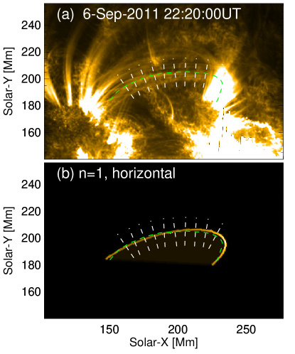
Figure 1: (a) FOV of AR 11283 (Event V) observed in the AIA 171 Å channel on 06 Sep 2011. (b) Synthetic view (Model V) in the 171 Å bandpass. The green dashed lines label the loop of interest (loop coordinate increases counter-clockwisely); while the set of white dashed segments denotes the slits used for time distance plots (Figure 2).

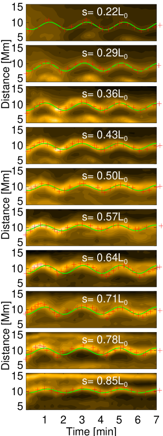
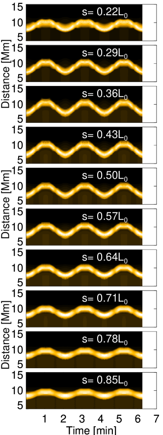
Figure 2: Left panel: time distance plots along slits normal to loop spine at selected loop coordinates in Event V. The crosses are the traced loop motions, while the green continuous line are the sinusoidal fits. Right panel: same as left panel, but extracted at the synthetic view for the $n=1$ horizontal mode (Model V).

Figure 3: Oscillation amplitude (a) and phase (b) as functions of the loop coordinate, measured in Event V and the $n=1$ horizontal mode (Model V), respectively.

2.2 Event and Model A

Event A was studied in detail by Aschwanden & Schrijver (2011). On 16 Oct 2010, a GOES-class M2.9 flare occurred at active region AR 11112. The excited coronal wave was observed to propagate to the north-west of AR 11112 and swept across the extended flare ribbons (Kumar et al. 2013). A bundle of coronal loops was located at a distance of about $0.32R_{\sun}$ to the disk centre (about $230\,\mathrm{Mm}$ north-west to AR 11112, Figure 4). Sequential brightening of the flare ribbons provided a good estimate of the Alfvén transit time, and therefore, the external Alfvén speed of the loop system was roughly measured (Aschwanden & Schrijver 2011). Two or more adjacent loops oscillated for about three to four cycles, no significant damping was observed. Moreover, the loop displacement appeared to exhibit a saw-tooth pattern (Figure 5), rather than sinusoidal curves as usually observed (Aschwanden et al. 2002).

Event A was claimed to be a vertical transverse loop oscillation observed by the AIA 171 Å channel (Aschwanden & Schrijver 2011). The loop length measured $163\,\mathrm{Mm}$; and the radius about $2.5\pm 0.3\,\mathrm{Mm}$. A bundle of loops connected two opposite polarities that were not associated with any sunspots. A potential field extrapolation gave a field strength of about $6\,\mathrm{G}$ at the loop apex; while the field value was measured at $4.0\pm 0.7\,\mathrm{G}$ using MHD seismology (Aschwanden & Schrijver 2011). The loop was filled with plasma of density of about $2\cdot 10^{8}\,\mathrm{cm^{-3}}$ and temperature of about $0.6\,\mathrm{MK}$. The oscillation period was about $6.3\,\mathrm{min}$; and the amplitude about $1.7\pm 0.4\,\mathrm{Mm}$. The measured parameters are listed in Table 1 (Event A).

We model the loop with a semi-toroidal geometry of a length at $L_{0}=160\,\mathrm{Mm}$ and a radius at $a=2.5\,\mathrm{Mm}$. The internal and external magnetic field is $B_{\text{i}}=4.0\,\mathrm{G}$ and $B_{\text{i}}=4.1\,\mathrm{G}$, respectively. The loop is filled with plasma of density at $2.2\cdot 10^{8}\,\mathrm{cm^{-3}}$, 12 times denser than the ambient plasma. The loop temperature is set at $0.57\,\mathrm{MK}$, 1.5 times hotter than the background. The plasma $\beta$ is about 0.054 and 0.003 for the internal and external plasma, respectively. This configuration gives a kink mode solution with $P_{0}=6.7\,\mathrm{min}$, obtained by solving the dispersion relationship (Equation 13 in Paper I, ). The oscillation amplitude is set at $\xi_{0}=4.5\,\mathrm{Mm}$ ($1.8a$).

We construct both horizontal and vertical kink wave models for this loop (Table 2, Model A). The best matching viewing angle is $[32^{\circ},135^{\circ}]$. The centre of the baseline is placed at $[646.2\arcsec,-274.8\arcsec]$; the synthetic image is interpolated in to AIA resolution and rotated by an angle of $5^{\circ}$ clockwisely.

Figure 5 illustrates the time distance plots along selected slits normal to the loop spine (Figure 4). The loop oscillations are coherently in phase along the loop, which confirms that the kink oscillation is an established eigenmode of the loop. The synthetic kink wave exhibits similar motions (Figure 5, middle and right columns). The horizontal mode finds intensity maxima when the loop oscillates to extreme positions, while the vertical mode reaches maxima when the loop crosses the equilibrium position. The phase and amplitude of the oscillation as functions of loop coordinates are measured and plotted in Figure 6.

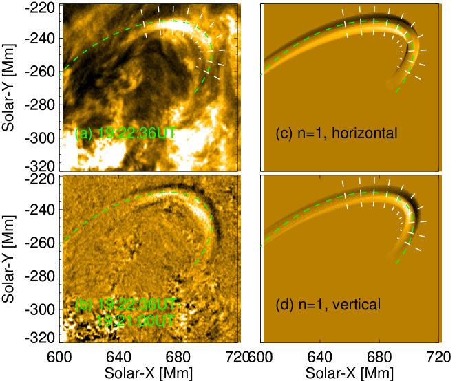
Figure 4: (a) FOV of Event A observed in the SDO/AIA 171 Å channel. (b) Difference image displaying the loop oscillation. (c) Difference image of the $n=1$ horizontal kink mode in the 171 Å bandpass. (d) Same as (c), but for the $n=1$ vertical mode. The green dashed lines in all panels label the approximate loop spine, the loop coordinate increases counter-clockwisely; while time-distance plots (Figure 5) are extracted along the set of white dashed slits.

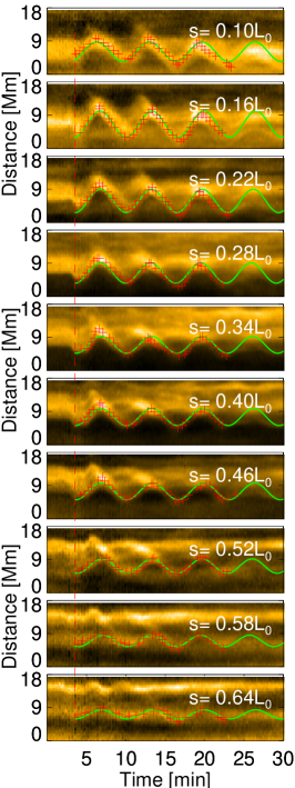
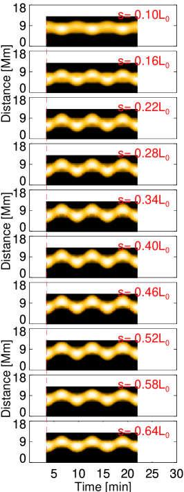
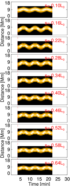
Figure 5: Time distance plots at selected loop coordinates extracted along the slits in the SDO/AIA 171 Å images during Event A (left column) and synthetic emission images for the $n=1$ horizontal (middle column) and vertical modes (right column). The red dashed line marks the start of oscillations; the crosses label the identified loop displacement; and the yellow continuous lines are the sinusoidal fits. The time starts at 19:10:00 UT 16 Oct 2010.

Figure 6: Oscillation amplitude (a) and phase (b) as functions of the loop coordinate, measured in Event A, the synthesised horizontal and vertical modes (Model A), respectively.

2.3 Event and Model W

AR 11121 was associated an Hale-class $\alpha$ sunspot group with a unipolar magnetic configuration, observed on the east limb of the solar disk on 03 Nov 2010. A GOES-class C3.4 flare started at about 12:12 UT and excited two EUV waves (see, e.g, Liu & Ofman 2014) or wave trains (e.g., Yuan et al. 2013). A magnetic flux tube that connected the main spot and another polarity was quickly filled up with hot and dense plasma (Figure 7). A kink loop oscillation was excited by the mass ejecta and exhibited non-coherent motions. Event W was a sporadic transverse oscillation of a flaring loop observed in the SDO/AIA channels that are sensitive to hot plasma emissions (131 Å, $\raise 0.73193pt\hbox{$\scriptstyle\sim$}10\,\mathrm{MK}$). The loop supported possible higher longitudinal overtones, and perhaps vertical polarisation of a kink wave (White et al. 2012).

White et al. (2012) performed 3D stereoscopy loop reconstruction combining the STEREO-B EUVI 195 Å bandpass and the SDO/AIA 131 Å channel. This procedure, using a low ($\raise 0.73193pt\hbox{$\scriptstyle\sim$}1.6\,\mathrm{MK}$) and a high ($\raise 0.73193pt\hbox{$\scriptstyle\sim$}10\,\mathrm{MK}$) temperature channel, may have overestimated the loop length by a factor of two, therefore, we measure the loop length by fitting a projected semi-torus to the loop (Figure 7(a)), and obtain a loop length of $L_{0}=240\,\mathrm{Mm}$. Differential emission measure (DEM) analysis using the forward-fitting technique (Aschwanden et al. 2013) gives the loop radius $a=3.8\,\mathrm{Mm}$, electron density $n_{e\text{i}}=3.2\cdot 10^{9}\,\mathrm{cm^{-3}}$, and loop temperature $T_{\text{i}}=10\,\mathrm{MK}$. The loop oscillated back and forth about every 5 min with an amplitude of about $4.7\,\mathrm{Mm}$ ($1.2a$).

To identify the overtone number, we constructed models of $n=2$ and $3$ overtones with options of either vertical and horizontal polarization (Figure 7). For the $n=2$ overtone, we use $B_{\text{i}}=11\,\mathrm{G}$ and $B_{\text{e}}=17\,\mathrm{G}$ as internal and external magnetic field strength. The flux tube is filled with plasma of $n_{e\text{i}}=2.5\cdot 10^{9}\,\mathrm{cm^{-3}}$ and $T_{\text{i}}=10\,\mathrm{MK}$, 4 times denser and 2 times hotter than the background. Therefore, the internal and external plasma $\beta$ are about $1.7$ and $0.08$, respectively, which are reasonable values for flaring loops (see, e.g., Van Doorsselaere et al. 2011a). In this configuration, the internal acoustic and Alfvén speeds are $C_{\text{s}\text{i}}=520\,\mathrm{km\,s^{-1}}$ and $V_{\text{A}\text{i}}=480\,\mathrm{km\,s^{-1}}$, while the external speeds are $C_{\text{s}\text{e}}=370\,\mathrm{km\,s^{-1}}$ and $V_{\text{A}\text{e}}=1600\,\mathrm{km\,s^{-1}}$, respectively. The kink mode solution gives the period $P_{0}=301\,\mathrm{s}$; the amplitude is set at $\xi_{0}=1.5\,\mathrm{Mm}$ ($0.5a$).

For the $n=3$ overtone, the internal and external magnetic field values are $B_{\text{i}}=9\,\mathrm{G}$ and $B_{\text{e}}=15\,\mathrm{G}$, respectively. The loop is filled with plasma at $n_{e\text{i}}=3.0\cdot 10^{9}\,\mathrm{cm^{-3}}$ and $T_{\text{i}}=10\,\mathrm{MK}$, 2 times denser and 2 times hotter than the ambient plasma. Then, the typical speeds are $C_{\text{s}\text{i}}=520\,\mathrm{km\,s^{-1}}$, $V_{\text{A}\text{i}}=360\,\mathrm{km\,s^{-1}}$, $C_{\text{s}\text{e}}=370\,\mathrm{km\,s^{-1}}$, and $V_{\text{A}\text{e}}=870\,\mathrm{km\,s^{-1}}$; and the internal and external plasma beta are 2.5 and 0.22, respectively. $P_{0}=277\,\mathrm{s}$ is the period of the kink mode solution. We used an oscillation amplitude at $\xi_{0}=1.5\,\mathrm{Mm}$ ($0.5a$).

The synthetic images of both $n=2$ and $n=3$ modes are interpolated into AIA resolution and aligned with AIA FOV by matching the centre of the loop baseline at $[-884.7\arcsec,-392.9\arcsec]$; then they are rotated by an angle of $-120^{\circ}$ clockwisely.

Figure 8 illustrates the time distance plots extracted from the AIA 131 Å observations and synthetic views of the $n=3$ horizontal and vertical overtones. We compare the oscillation amplitude and phase distribution along the loop coordinate and attempt to identify the loop node (Figure 9).

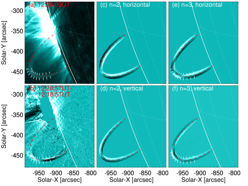
Figure 7: (a) FOV of AR 11121 observed at the South-East solar limb by the SDO/AIA 131 Å channel. The dashed line labels the hot flaring loop of interest. (b) Difference images made by subtracting two images taken at about half an oscillation cycle apart. (c) - (f) Difference images of two synthetic images taken at half a wave cycle apart for $n=2$ horizontal and vertical overtones, and $n=3$ horizontal and vertical overtones, respectively.

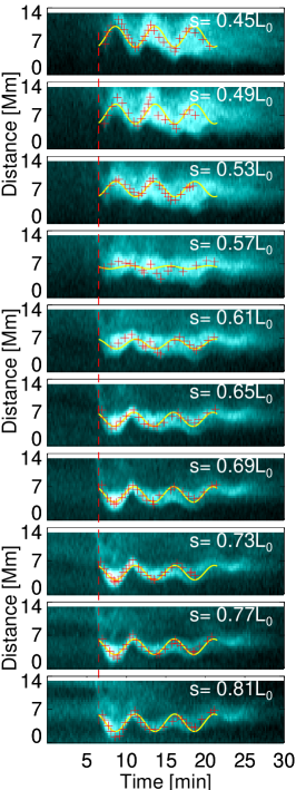
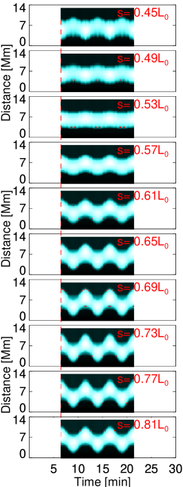
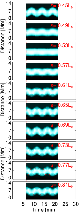
Figure 8: Left panel: time distance plots along slits normal to the loop spine at selected loop coordinates at Event W. The crosses are the traced loop motions, while the green continuous lines are the sinusoidal fits. Middle and right panels: same as left panel, but extracted at the synthetic loop views for the $n=3$ horizontal and vertical modes, respectively (Model W).

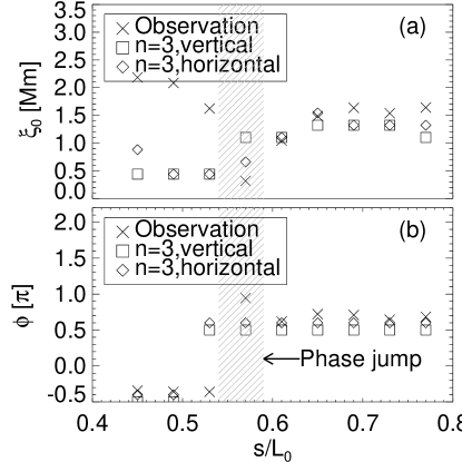
Figure 9: Amplitude (a) and phase (b) of the loop oscillation as functions of loop coordinate, measured in observation (Event W) and the $n=3$ horizontal and vertical modes (Model $\text{W}_{3}$), respectively. The hatched areas highlight a $180^{\circ}$-phase jump.

Table 1: List of transverse loop oscillations

Kink wave	Event V	Event A	Event W
Active region	AR 11283	AR 11112	11121
Date of observation	06 Sep 2011	16 Oct 2010	03 Nov 2010
Time interval of observation	22:19-22:30 UT	19:13-19:35 UT	12:10-12:40 UT
Flare class (start time)	X2.1 (22:12 UT)	M2.9 (19:07 UT)	C3.4 (12:12 UT)
EUV channel	171 Å	171 Å	131 Å and 94 Å
Characteristic temperature $\,\mathrm{[MK]}$	0.6	0.6	10
Longitudinal mode number $n$	1	1	2 or 3
Polarisation: horizontal (H) or vertical (V) ?	H	V	H or V
Loop length $L_{0}\,\mathrm{[Mm]}$	$160\pm 20$	163	240
Loop radius $a\,\mathrm{[Mm]}$	0.85	$2.5\pm 0.3$	3.8
Internal magnetic field $B_{\text{i}}\,\mathrm{[G]}$	32-41	$4.0\pm 0.7$	$\cdots$
Internal plasma density $\rho_{\text{i}}\,\mathrm{[10^{-12}kg\,m^{-3}]}$	1.2	$0.32\pm 0.05$	5.4
Internal electron density $n_{e\text{i}}\,\mathrm{[10^{9}cm^{-3}]}$	$\raise 0.73193pt\hbox{$\scriptstyle\sim$}0.7$	$0.19\pm 0.03$	3.2
Density ratio $\rho_{\text{i}}/\rho_{\text{e}}$	1.0-3.3	11-14	$\cdots$
Internal temperature $T_{\text{i}}\,\mathrm{[10^{6}K]}$	0.8	$0.57\pm 0.14$	10
Internal Alfvén speed $V_{\text{A}\text{i}}\,\mathrm{[km\,s^{-1}]}$	1860-2620	$560\pm 100$	$\cdots$
External Alfvén speed $V_{\text{A}\text{e}}\,\mathrm{[km\,s^{-1}]}$	$\cdots$	$1940\pm 100$	$\cdots$
Oscillation period $P_{0}\,\mathrm{[s]}$	$122\pm 6$	$370\pm 30$	$302\pm 14$
Amplitude of displacement $\xi_{0}\,\mathrm{[Mm]}$	0.9-2.9 ($1.0a$-$3.4a$)	1.4-2.2 (0.56a-0.88a)	4.7 (1.2a)

Table 2: Parameters of the loop systems and the standing kink modes

Loops	Model V	Model A	Model $\text{W}_{1}$	Model $\text{W}_{2}$	Model $\text{W}_{3}$
Loop length $L_{0}\,\mathrm{[Mm]}$	160	163	240	240	240
Loop radius $a\,\mathrm{[Mm]}$	0.85	2.5	3.0	3.0	3.0
Internal magnetic field $B_{\text{i}}\,\mathrm{[G]}$	30	4.0	25	11	9.0
External magnetic field $B_{\text{e}}\,\mathrm{[G]}$	30	4.1	28	17	15
Internal plasma density $\rho_{\text{i}}\,\mathrm{[10^{-12}kg\,m^{-3}]}$	1.67	0.37	4.2	4.2	5.0
Internal electron density $n_{e\text{i}}\,\mathrm{[10^{9}cm^{-3}]}$	1.0	0.22	2.5	2.5	3.0
Density ratio $\rho_{\text{i}}/\rho_{\text{e}}$	3.0	12	6.0	5.0	2.0
Internal temperature $T_{\text{i}}\,\mathrm{[10^{6}K]}$	0.8	0.57	10	10	10
Temperature ratio $T_{\text{i}}/T_{\text{e}}$	1.5	1.5	2.0	2.0	2.0
Internal plasma beta $\beta_{i}$	0.0062	0.054	0.27	1.4	2.5
External plasma beta $\beta_{e}$	0.0014	0.0029	0.018	0.06	0.22
Internal acoustic speed $C_{\text{s}\text{i}}\,\mathrm{[km\,s^{-1}]}$	150	130	520	520	520
Internal Alfvén speed $V_{\text{A}\text{i}}\,\mathrm{[km\,s^{-1}]}$	2100	590	1090	480	360
External acoustic speed $C_{\text{s}\text{e}}\,\mathrm{[km\,s^{-1}]}$	120	100	370	370	370
External Alfvén speed $V_{\text{A}\text{e}}\,\mathrm{[km\,s^{-1}]}$	3600	2100	3000	1600	870
Longitudinal mode number $n$	1	1	1	2	3
Period $P_{0}\,\mathrm{[s]}$	126	403	317	303	277
Amplitude of displacement $\xi_{0}\,\mathrm{[Mm]}$	1.9 ($2.2a$)	4.5 ($1.8a$)	1.5 (0.5a)	1.5 (0.5a)	1.5 ($0.5a$)
Amplitude of velocity perturbation $\hat{v}\,\mathrm{[km\,s^{-1}]}$	100	70 42		30	35
Relative amplitude of density perturbation $\hat{\rho}_{1}/\rho_{\text{i}}$	0.0003	0.003	0.0006	0.003	0.005
Relative amplitude of temperature perturbation $\hat{T}_{1}/T_{\text{i}}$	0.0002	0.002	0.0004	0.002	0.003
AIA channel	171 Å	171 Å	131 Å	131 Å	131 Å
Polarisation: horizontal (H) or vertical (V) ?	H	H & V	H & V	H & V	H & V
Viewing angle $[\tau,\eta]$	$[30^{\circ},130^{\circ}]$	$[32^{\circ},135^{\circ}]$	$[90^{\circ},25^{\circ}]$	$[90^{\circ},25^{\circ}]$	$[90^{\circ},25^{\circ}]$
Centre of the loop baseline	$[226.3\arcsec,215.3\arcsec]$	$[646.2\arcsec,-274.8\arcsec]$	$[-884.7\arcsec,-392.9\arcsec]$
Rotation angle of synthetic image (clockwise)	$3^{\circ}$	$5^{\circ}$	$-120^{\circ}$	$-120^{\circ}$	$-120^{\circ}$

3 Applications

3.1 Mode identification

Event V is a horizontally polarised fundamental kink mode, given the simple geometry and projection (Figure 1). The time distance plot of the synthetic data are consistent with the observation (Figure 2): the oscillations at different position of the loop are coherently in phase, and the emission intensity maxima are found when the loop oscillates to the extreme positions.

Figure 4 compares the difference images of Event A and synthetic data of the $n=1$ horizontal and vertical polarisations. The vertical mode agrees better with the observation: it stretches the loop geometry; and the oscillation phase remains unchanged in this viewing angle (Figure 4(d)). In the horizontal mode, the oscillation phase jumps by $180^{\circ}$ at the right leg owing to the LOS effect. The maxima of emission intensity could not be effectively measured in observation, therefore, no further information could be extracted from the intensity variation owing to the contamination of other loops (Figure 5).

In Event W, one leg of the loop blended into the background and could not be effectively identified; however the rest of the loop gave a possible geometry for the missing leg (Figure 7(a)). By comparing the difference images of Event W and Model W, one could tell that both the $n=3$ horizontal and vertical modes agree with the observation (Figure 7), while the $n=2$ modes do not give the right position of the node. The left panel of Figure 8 illustrates that the emission intensity reached maxima when the loop oscillated to extreme positions; it implies that the horizontal polarisation is more likely to be the right mode. In the follow-up analysis of this event, we, henceforth, only consider the $n=3$ modes.

3.2 Amplitude and phase distribution

Figure 3 compares the amplitude and phase distribution of Event V and Model V. Model V reproduces the general trend of amplitude distribution along the loop and successfully matches the location of maximum amplitude. The phase extracted in Model V is constant at the selected loop coordinate, while those measured in the observation scatters around the synthetic values.

Figure 6 presents the case of Event A and Model A. The $n=1$ vertical mode reproduces Event A better: both the general profile and the position of maximum displacement. Again, the match between the phases of the observation and models is excellent. However, close to the footpoint, the horizontal mode exhibits a $180^{\circ}$ phase jump, as also illustrated in Figure 4. Near the footpoint, the observational errors are large in the phase, and thus, this can not be used to distinguish the mode.

Figure 9 studies the case of Event W and Model W. Since we already determined the longitudinal overtone (see Section 3.1), only two polarisations of the $n=3$ modes are plotted. The amplitude finds a minimum at a node around $s/L_{0}=0.54-0.59$, the horizontal mode reproduces this minimum at a close position. The phase jump is also well modelled by both modes. By considering the difference images (Figure 7) and the profile of the oscillation amplitude (Figure 9(a)), we conclude that the $n=3$ horizontal mode agrees better with the Event W than the other modes.

3.3 Loop intensity and width oscillations

In Paper I, we show that a quadrupole term in the kink mode could deform the loop cross-section, and thus, the loop width is liable to a periodic modulation at half of the kink mode period. In spectral observations, the non-thermal spectral line broadening, caused by the quadrupole term, leads to line intensity suppression at loop edges, so it further enhances the effective loop width modulation. In imaging observations, the line intensity suppression at loop edges does not exist, however, if the loop displacement is large enough, this effect could also be observed. In Event V, the loop of interest was clear from background contamination, and it had an displacement at the order of two loop radii. Therefore, Event V is selected to demonstrate the loop width modulation effect. We extracted the time series of the loop displacement, normalised flux and width variation at $s=0.5L_{0}$, and measured the oscillation period with Lamb-Scargle periodogram (see, e.g., Scargle 1982; Horne & Baliunas 1986; Yuan et al. 2011).

The loop oscillated back and forth about every $2\,\mathrm{min}$ with an amplitude of about $2\,\mathrm{Mm}$ (Figure 10 (a) and (b)). The modelled loop oscillation reproduces similar amplitude and periodicity (Figure 11 (a) and (b)).

The normalized flux also has periodic variations, and the power spectrum exhibits a prominent peak at $1.8\pm 0.2\,\mathrm{min}$ (Figure 10 (c) and (d)), which has a False Alarm Probability (FAP, see Horne & Baliunas 1986; Yuan et al. 2011, for definition) or a significance level less than 0.05. The peak value is consistent with the oscillation period of the kink oscillation, if we consider the $1\sigma$ error bar ($1.6-2.0\,\mathrm{min}$ vs $1.9-2.4\,\mathrm{min}$) and the coarse resolution of the spectra. The modulation depth is about 20% of the average loop intensity. In the synthetic loop oscillation, the flux also shows the period of the kink oscillation, but also its harmonics at $0.52\,\mathrm{min}$ and $1.0\,\mathrm{min}$. The strongest periodicity is at $0.52\pm 0.02\,\mathrm{min}$, this may be due to the complex motions of the quasi-rigid kink oscillations, the quadrupole terms and the breaking of symmetry due to the LOS effect. The lack of this period in the observation may be cause of lower time resolution, therefore, we do a four-point moving average on the times series and re-calculate the power spectrum (blue lines in Figure 11 (c) and (d)). Now the periodicity at $2.1\pm 0.3\,\mathrm{min}$ become more prominent and is more consistent with observation.

The loop width was also measured and appears to vary with a clear periodicity. The amplitude is about $0.15\,\mathrm{Mm}$ ($0.17a$), about 15% of the loop displacement. The order of magnitude is consistent with the measurement in Paper I. Two peaks in the spectrum are measured at $2.3\pm 0.5\,\mathrm{min}$ and $1.0\pm 0.1\,\mathrm{min}$, respectively, although they are below the value of $95\%$-confidence level, but the periodicities are clearly seem in the time series, albeit for only 2-3 cycles. In the synthetic data, these two peaks are significantly measured. Other higher harmonics are also seen. As we have much better time resolution, we are able to measure more details of kink oscillations, which is beyond the detectability of modern instrument.

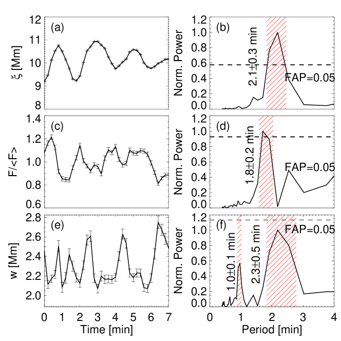
Figure 10: (a),(c) and (e) are the time series of loop displacement $\xi$, normalised emission flux $F/<F>$,and loop width $w$, measured at $s=0.5L_{0}$ in Event V, respectively; while (b), (d) and (f) are the corresponding spectra. The dashed lines mark the relevant false alarm probability (FAP) at 0.05. The hatched areas highlight the prominent oscillation periods.

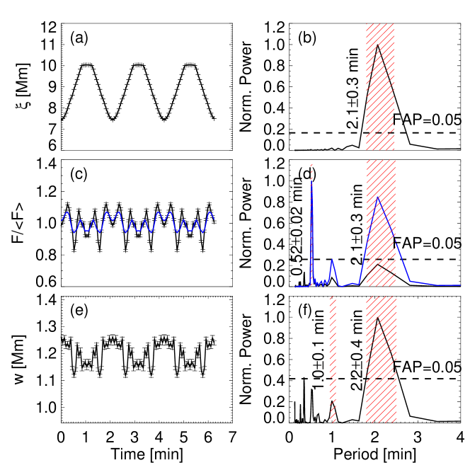
Figure 11: Same as Figure 10, but for Model V. In panel (c), the blue continuous line plots the 4-point running average of normalised flux; and the power spectrum (blue line) has enhanced peaks in long-period range.

4 Conclusions

In this paper, we demonstrated how forward models can be used to understand observational data of transverse loop oscillations. Three events were selected and forward modelled to reproduce the SDO/AIA imaging observations. We have performed mode identification to determine the oscillation polarisation and overtone. Moreover, we measured the amplitude and phase distribution along the loop, and the loop intensity and width oscillations, and compared them with observations.

Longitudinal overtone could be identified by comparing difference images of the observational and synthetic data, and further clues could be obtained by identifying and matching the nodes in amplitude and phase distributions along the loop. The polarisation could not be effectively fixed by difference images alone. However, a key point is where the loop intensity variation reaches its maxima. The horizontal mode finds its maxima when the loop oscillates to extreme positions, while for the vertical mode, maxima are reached when the loop sweeps across the equilibrium position.

The longitudinal amplitude distribution could only be reproduced quantitatively as a general trend. On the other hand, our models could reproduce the longitudinal phase distribution very well for both the fundamental mode and higher overtones.

In our forward modelling, the loop intensity flux is found to oscillate with multiple periodic components, which are basically the kink oscillation period and its 2nd and 4th overtones. If the time resolution allows, the 4th overtone could have the strongest power. However, with AIA, one may only observe the fundamental mode and its 2nd overtone. But, if the kink oscillation period is longer, then the 4th overtone may be resolved as well.

For loops without background contamination, the loop width is measured to vary periodically, at both the fundamental kink period and its 2nd overtone. Our models also reproduce these periodicities. However, other higher overtones are also possible to detect, if the instrument capability allows.

Our model has reproduced many interesting features of kink oscillations, many of them still await for rigid detection with modern instruments. Forward modelling could assist in measuring overtone mode number, identifying polarisation, investigating the amplitude and phase distribution, and predict the possible origin of intensity and width variations.

References

- Anfinogentov et al. (2013) Anfinogentov, S., Nisticò, G., & Nakariakov, V. M. 2013, A&A, 560, A107
- Anfinogentov et al. (2015) Anfinogentov, S. A., Nakariakov, V. M., & Nisticò, G. 2015, A&A, 583, A136
- Antolin & Van Doorsselaere (2013) Antolin, P., & Van Doorsselaere, T. 2013, A&A, 555, A74
- Arregui et al. (2007) Arregui, I., Andries, J., Van Doorsselaere, T., Goossens, M., & Poedts, S. 2007, A&A, 463, 333
- Aschwanden et al. (2013) Aschwanden, M. J., Boerner, P., Schrijver, C. J., & Malanushenko, A. 2013, Sol. Phys., 283, 5
- Aschwanden et al. (2002) Aschwanden, M. J., de Pontieu, B., Schrijver, C. J., & Title, A. M. 2002, Sol. Phys., 206, 99
- Aschwanden et al. (1999) Aschwanden, M. J., Fletcher, L., Schrijver, C. J., & Alexander, D. 1999, ApJ, 520, 880
- Aschwanden et al. (2003) Aschwanden, M. J., Nightingale, R. W., Andries, J., Goossens, M., & Van Doorsselaere, T. 2003, ApJ, 598, 1375
- Aschwanden & Schrijver (2011) Aschwanden, M. J., & Schrijver, C. J. 2011, ApJ, 736, 102
- Boerner et al. (2012) Boerner, P., Edwards, C., Lemen, J., et al. 2012, Sol. Phys., 275, 41
- Chen & Peter (2015) Chen, F., & Peter, H. 2015, A&A, 581, A137
- Chen et al. (2011) Chen, Y., Feng, S. W., Li, B., et al. 2011, ApJ, 728, 147
- Chen et al. (2010) Chen, Y., Song, H. Q., Li, B., et al. 2010, ApJ, 714, 644
- De Moortel & Nakariakov (2012) De Moortel, I., & Nakariakov, V. M. 2012, Royal Society of London Philosophical Transactions Series A, 370, 3193
- De Moortel & Pascoe (2009) De Moortel, I., & Pascoe, D. J. 2009, ApJ, 699, L72
- Edwin & Roberts (1983) Edwin, P. M., & Roberts, B. 1983, Sol. Phys., 88, 179
- Goossens et al. (2014) Goossens, M., Soler, R., Terradas, J., Van Doorsselaere, T., & Verth, G. 2014, ApJ, 788, 9
- He et al. (2009) He, J., Marsch, E., Tu, C., & Tian, H. 2009, ApJ, 705, L217
- Horne & Baliunas (1986) Horne, J. H., & Baliunas, S. L. 1986, ApJ, 302, 757
- Jess et al. (2015) Jess, D. B., Morton, R. J., Verth, G., et al. 2015, Space Sci. Rev., 190, 103
- Kumar et al. (2013) Kumar, P., Cho, K.-S., Chen, P. F., Bong, S.-C., & Park, S.-H. 2013, Sol. Phys., 282, 523
- Lemen et al. (2012) Lemen, J. R., Title, A. M., Akin, D. J., et al. 2012, Sol. Phys., 275, 17
- Liu & Ofman (2014) Liu, W., & Ofman, L. 2014, Sol. Phys., 289, 3233
- Nakariakov et al. (2009) Nakariakov, V. M., Aschwanden, M. J., & van Doorsselaere, T. 2009, A&A, 502, 661
- Nakariakov & Ofman (2001) Nakariakov, V. M., & Ofman, L. 2001, A&A, 372, L53
- Nakariakov et al. (1999) Nakariakov, V. M., Ofman, L., Deluca, E. E., Roberts, B., & Davila, J. M. 1999, Science, 285, 862
- Nakariakov & Verwichte (2005) Nakariakov, V. M., & Verwichte, E. 2005, Living Reviews in Solar Physics, 2, 3
- Nisticò et al. (2013) Nisticò, G., Nakariakov, V. M., & Verwichte, E. 2013, A&A, 552, A57
- Pascoe & De Moortel (2014) Pascoe, D. J., & De Moortel, I. 2014, ApJ, 784, 101
- Scargle (1982) Scargle, J. D. 1982, ApJ, 263, 835
- Schrijver et al. (2002) Schrijver, C. J., Aschwanden, M. J., & Title, A. M. 2002, Sol. Phys., 206, 69
- Van Doorsselaere et al. (2011a) Van Doorsselaere, T., De Groof, A., Zender, J., Berghmans, D., & Goossens, M. 2011a, ApJ, 740, 90
- Van Doorsselaere et al. (2011b) Van Doorsselaere, T., Wardle, N., Del Zanna, G., et al. 2011b, ApJ, 727, L32
- Verwichte et al. (2013) Verwichte, E., Van Doorsselaere, T., Foullon, C., & White, R. S. 2013, ApJ, 767, 16
- Wang et al. (2008) Wang, T. J., Solanki, S. K., & Selwa, M. 2008, A&A, 489, 1307
- White et al. (2012) White, R. S., Verwichte, E., & Foullon, C. 2012, A&A, 545, A129
- Yuan et al. (2011) Yuan, D., Nakariakov, V. M., Chorley, N., & Foullon, C. 2011, A&A, 533, A116
- Yuan et al. (2014a) Yuan, D., Nakariakov, V. M., Huang, Z., et al. 2014a, ApJ, 792, 41
- Yuan et al. (2015a) Yuan, D., Pascoe, D. J., Nakariakov, V. M., Li, B., & Keppens, R. 2015a, ApJ, 799, 221
- Yuan et al. (2013) Yuan, D., Shen, Y., Liu, Y., et al. 2013, A&A, 554, A144
- Yuan et al. (2014b) Yuan, D., Sych, R., Reznikova, V. E., & Nakariakov, V. M. 2014b, A&A, 561, A19
- Yuan & Van Doorsselaere (2015) Yuan, D., & Van Doorsselaere, T. 2015, submitted to ApJS
- Yuan et al. (2015b) Yuan, D., Van Doorsselaere, T., Banerjee, D., & Antolin, P. 2015b, ApJ, 807, 98
- Zimovets & Nakariakov (2015) Zimovets, I. V., & Nakariakov, V. M. 2015, A&A, 577, A4