A see-saw scenario of an $A_{4}$ flavour symmetric
standard model

Abstract

A see-saw scenario for an $A_{4}$ flavour symmetric standard model is presented. The latter, compared with the standard model, has an extended field content adopting now an additional $A_{4}$ symmetry structure (along with the standard model symmetry). As before, the see-saw mechanism can be realized in several models of different types depending on different ways of neutrino mass generation corresponding to the introduction of new (heavy in general) fields with different symmetry structures. In the present paper, a general description of all these see-saw types is made with a more detailed investigation on type-I models, while for type-II and type-III models a similar strategy can be followed. As within the original see-saw mechanism, the symmetry structure of the standard model fields decides the number and the symmetry structure of the new fields. In a model considered here, the scalar sector consists of three standard-model-Higgs-like iso-doublets ($SU_{L}(2)$-doublets) forming together an $A_{4}$-triplet, and three iso-singlets transforming as three singlets (1,$1^{{}^{\prime}}$ and $1^{{}^{\prime\prime}}$) of $A_{4}$. In the lepton sector, the three left-handed lepton iso-doublets form an $A_{4}$-triplet, while the three right-handed charged leptons are either $A_{4}$-singlets in one version of the model, or components of an $A_{4}$-triplet in another version. To generate neutrino masses through, say, the type-I see-saw mechanism, it is natural to add four right-handed neutrino multiplets, including one $A_{4}$-triplet and three $A_{4}$-singlets. For an interpretation, the model is applied to deriving some physics quantities such as neutrinoless double beta decay effective mass $|\langle m_{ee}\rangle|$, CP violation phase $\delta_{CP}$ and Jarlskog parameter $J_{CP}$, which can be verified experimentally.

I Introduction

Although the standard model (SM) sm1 ; sm2 ; qft ; quangyem has proved to be a very successful model of elementary particles and their interactions, especially after the discovery of the Brout-Englert-Higgs boson, or, shortly, the Higgs boson, by the LHC collaborations ATLAS and CMS Aad:2012tfa ; Chatrchyan:2012ufa (see also Ky:2015eka for a review), it, however, cannot solve a number of problems in particle physics and astrophysics. One of such problems is that of neutrino masses and mixing which is an experimental fact. These problems often require an extension of the SM. Among many extended, or say, beyond standard model (BSM), models, suggested, the models based on a flavour symmetry have attracted much interest for over one decade. In these models, the original SM fields, including neutrinos, along with new fields which may be added, are assumed to adopt a flavour symmetry (transformation) structure.

In the SM, neutrinos are massless and not mixing, but experimental results on neutrino oscillations Fukuda:1998tw ; Fukuda:1998ub ; Fukuda:1998mi ; Ahmad:2001an ; Ahmad:2002jz ; Ahmad:2002ka have shown that neutrinos are massive and mixing. A flavour neutrino, thus, is a mixture of light neutrinos $\nu_{i}$ (where $i=1,2,3$, for a three-neutrino model) with masses, say $m_{i}$, expected so far to be smaller than $1$ eV (see, e.g., Olive:2016xmw ). The (three-neutrino) mixing matrix in the canonical form, known as Pontecorvo-Maki-Nakagawa-Sakata (PMNS) neutrino mixing matrix, and parametrized by three mixing angles, $\theta_{12}$, $\theta_{23}$, $\theta_{13}$, one Dirac phase $\delta$ and, if neutrinos are Majorana particles, two more Majorana phases, $\alpha_{21}$ and $\alpha_{31}$, can be written in the form

$$U_{PMNS}=U\times P,$$ (1)

where

$$P={\rm diag}(e^{i\alpha_{21}/2},e^{i\alpha_{31}/2},1),$$ (2)

and

$$U=\left(\begin{array}[]{ccc}c_{12}c_{13}&s_{12}c_{13}&s_{13}e^{-i\delta}\\ -c_{23}s_{12}-s_{13}s_{23}c_{12}e^{i\delta}&c_{23}c_{12}-s_{13}s_{23}s_{12}e^{i\delta}&s_{23}c_{13}\\ s_{23}s_{12}-s_{13}c_{23}c_{12}e^{i\delta}&-s_{23}c_{12}-s_{13}c_{23}s_{12}e^{i\delta}&c_{23}c_{13}\end{array}\right),$$ (3)

with the notations $s_{ij}=\sin\theta_{ij}$ and $c_{ij}=\cos\theta_{ij}$, $1\leq i<j\leq 3$, used. Here, the mixing angles and the phases are taken within the following ranges: $\theta_{ij}\in[0,\pi/2]$, $\delta\in[0,2\pi]$, $\alpha_{j1}\in[0,2\pi]$, $j=2,3$. As the Dirac phase $\delta$ is related to the CP violation (CPV) phenomenon, it is also called the CPV phase and denoted as $\delta_{CP}$ (but below the short notation $\delta$ is more frequently used). The best fit values of the neutrino oscillation angles, given in Olive:2016xmw ; Capozzi:2017ipn ; Esteban:2016qun , are close to the tri-bi-maximal (TBM) mixing, where $\sin^{2}\theta_{12}^{\tiny{TBM}}=1/3$, $\sin^{2}\theta_{23}^{TBM}=1/2$ and $\sin^{2}\theta_{13}^{TBM}=0$ Harrison:2002er . The most recent neutrino oscillation experimental data Olive:2016xmw ; Capozzi:2017ipn ; Esteban:2016qun , summarized in Table 1 for both the normal ordering (NO) and the inverse ordering (IO) of neutrino masses, has shown, however, a deviation of the PMNS matrix from the TBM form. There have been many attempts, including an assumption of a flavour symmetry (see more details below), to explain this phenomenon.

Parameter	Best fit	$1\sigma$ range	$2\sigma$ range	$3\sigma$ range
$\Delta m_{21}^{2}/10^{-5}~{}\mathrm{eV}^{2}$ (NO or IO)	7.54	7.32 – 7.80	7.15 – 8.00	6.99 – 8.18
$\sin^{2}\theta_{12}/10^{-1}$ (NO or IO)	3.08	2.91 – 3.25	2.75 – 3.42	2.59 – 3.59
$\Delta m_{31}^{2}/10^{-3}~{}\mathrm{eV}^{2}$ (NO)	2.47	2.41 – 2.53	2.34 – 2.59	2.27 – 2.65
$|\Delta m_{32}^{2}|/10^{-3}~{}\mathrm{eV}^{2}$ (IO)	2.42	2.36 – 2.48	2.29 – 2.55	2.23 – 2.61
$\sin^{2}\theta_{13}/10^{-2}$ (NO)	2.34	2.15 – 2.54	1.95 – 2.74	1.76 – 2.95
$\sin^{2}\theta_{13}/10^{-2}$ (IO)	2.40	2.18 – 2.59	1.98 – 2.79	1.78 – 2.98
$\sin^{2}\theta_{23}/10^{-1}$ (NO)	4.37	4.14 – 4.70	3.93 – 5.52	3.74 – 6.26
$\sin^{2}\theta_{23}/10^{-1}$ (IO)	4.55	4.24 – 5.94	4.00 – 6.20	3.80 – 6.41

Table 1: The best-fit values and $n\sigma$ allowed ranges of the 3-neutrino oscillation parameters for a normal neutrino mass ordering (NO) and an inverse neutrino mass ordering (IO) Olive:2016xmw ; Capozzi:2017ipn ; Esteban:2016qun .

Besides the parameters in the PMNS mixing matrix, neutrino oscillation experiments also allow us to determine the neutrino squared mass differences $\Delta m_{21}^{2}$ and $\Delta m_{31}^{2}$. Although the absolute neutrino masses have not yet been known but it is believed that they are very tiny, less than 1 eV, as said above. Therefore, one needs to understand why the neutrinos, compared with the charged leptons, are so light, and find a mechanism for generation of such small masses. A very popular mechanism of this kind is called the see-saw mechanism which can generate a small neutrino mass due to an introduction of a larger scale which could be a mass of a heavy, compared with neutrinos, BSM particle. The see-saw mechanism, appearing first as type I in Minkowski:1977sc ; GellMann:1980vs ; Mohapatra:1979ia ; Schechter:1980gr ; Schechter:1981cv , has been originally applied to the SM (see Bilen ; Mohapatra:1998rq for later developments and a more complete presentation) but a natural question arising here is whether this mechanism can be incorporated in a model with an additional symmetry. This idea has attracted interest of other authors investigating different models, including those with a flavour symmetry adopted (see, for example, Caldwell:1993kn ; Petcov:1993rk ).

Various models with flavour symmetries have been introduced to explain the mass spectrum and the mixing matrix of the quarks and leptons. Among them, the models constructed with non-Abelian discrete flavour symmetries added are investigated quite intensively (see King:2014nza ; Ishimori:2010au ; Altarelli:2010gt for a review). Especially, a number of models that are not only able to give a TBM mixing as well as adjustable to fit the data of the observed neutrino oscillations but also interesting due to their simplicity, are based on the $A_{4}$ flavour symmetry Ishimori:2010au ; Altarelli:2010gt ; Ma:2001dn ; Ma:2002iq ; Babu:2002dz ; Ma:2004zv ; Altarelli:2009kr ; Parattu:2010cy ; King:2011ab ; Altarelli:2012bn ; Altarelli:2012ss ; Ferreira:2013oga ; Barry:2010zk ; Ahn:2012tv ; Felipe:2013vwa ; Hernandez:2013dta ; Varzielas:2015joa ; Hung:2015nva ; Ky:2016rzl . There are many models based on other flavour symmetries but they are beyond the scope of this paper.

In the present work, a “naturally” extended see-saw version of the SM adopting an $A_{4}$ flavour symmetry is suggested and considered. In this model the three generations of the left-handed leptons are grouped in a triplet of $A_{4}$, while the three right-handed charged leptons either transform under $A_{4}$ as its 1, $1^{{}^{\prime}}$ and $1^{{}^{\prime\prime}}$ singlets (but there is another version, in which the right-handed charged leptons form an $A_{4}$ triplet). The scalar sector is extended with the SM Higgs boson acquiring now an $A_{4}$ triplet structure and three additional scalar iso-singlets transforming as 1, $1^{{}^{\prime}}$ and $1^{{}^{\prime\prime}}$ singlets of $A_{4}$. Light neutrino masses can be generated via the type I see-saw mechanism by introducing four right-handed neutrinos, which are one triplet and three singlets $(1,1^{\prime},1^{\prime\prime})$ under the transformation of the $A_{4}$ group. This model is a multiple model of several copies corresponding to different representations of $A_{4}$. To our knowledge, this approach is done for the first time here, and it reminds of the co-variant diagram approach in supersymmetry models Gates:1983nr ; Grisaru:1984ja ; Galperin:1987vx ; Ky:1988yn .

In Section 2 we present the main idea of the original see-saw mechanism applied to the SM and extend it to the case with a flavour symmetry involved. Sections 3 and 4 are devoted to a more detailed investigation on a type I see-saw mechanism within the newly suggested $A_{4}$-flavour symmetric SM which is checked by calculating some physics quantities for neutrino masses and mixing and comparing them with the current experimental data.
Section 5 is designed for some comments and conclusion. The bibliography of the cited works may be still far from being complete but we hope it gives a general view on the development of the topic considered here. Before going to physics details in the sections following, the reader can have a look at the appendix for notations and a quick review on the basic elements of $A_{4}$ representations.

II See-saw mechanism for an $A_{4}$-flavour symmetric standard model

Neutrinos in the standard model (SM) are massless but, as said above, experimental results Fukuda:1998tw ; Fukuda:1998ub ; Fukuda:1998mi ; Ahmad:2001an ; Ahmad:2002jz ; Ahmad:2002ka have shown that they have masses though very tiny. The see-saw mechanism Bilen ; Mohapatra:1998rq is an attempt to explain the neutrino mass smallness. Let us first recall the see-saw mechanism applied to the (original) SM. Generally speaking, this mechanism imposes an extension on the SM by adding in different ways new (heavy in general) fields in order to generate (small effective) masses of neutrinos (due to big masses of the new fields). These ways of neutrino mass generation are called see-saw models referred below to as classical or pre-flavour symmetric see-saw models.

II.1 Pre-flavour-symmetric see-saw models

There are three types of classical see-saw models: I, II and III, corresponding to three ways of neutrino mass generation, requiring an introduction of three kinds of new fields which in general are heavy. The see-saw I generates neutrino masses with the introduction of a lepton iso-singlet (a right-handed neutrino), while the generation of neutrino masses via the see-saw II and III requires respectively a new scalar iso-triplet and a new lepton iso-triplet to be introduced. Let us look at a closer distance how they work.

A neutrino mass could be of Dirac- or Majorana type. A general Lagrangian neutrino mass term, denoted below by $\mathcal{L}_{m_{\nu}}$, has the form

$$\mathcal{L}_{m_{\nu}}=-\frac{1}{2}\overline{n}_{L}M_{\nu}(n_{L})^{c}+h.c.,$$ (4)

where

$$n_{L}=\begin{pmatrix}\nu_{L}\\ (N_{R})^{c}\\ \end{pmatrix}$$ (5)

is a neutrino pattern, and

$$M_{\nu}=\left(\begin{array}[]{cc}M_{L}&M_{D}\\ (M_{D})^{T}&M_{R}\\ \end{array}\right)$$ (6)

is a neutrino mass matrix ($M_{L}$ is a $3\times 3$ matrix for the case of three left-handed neutrinos $\nu_{L}$, and $M_{R}$ is an $n\times n$ matrix for the case of $n$ right-handed neutrinos $N_{R}$, then $M_{D}$ is a $3\times n$ matrix). If $M_{L}\ll M_{R}$, the matrix (6) can be approximately diagonalized in the block form Bilen ; Mohapatra:1998rq

$$M_{\nu}=\left(\begin{array}[]{cc}M_{1}&0\\ 0&M_{2}\\ \end{array}\right),$$ (7)

where $M_{1}$ and $M_{2}$,

$$\begin{cases}M_{1}\approx M_{L}-(M_{D})^{T}(M_{R})^{-1}M_{D},\\ M_{2}\approx M_{R},\end{cases}$$ (8)

are complex matrices and they are the mass matrices of the light- and heavy neutrinos, respectively. The light neutrinos, which are (mostly) left-handed and can interact with ordinary SM fields, are called active neutrinos, while the heavy, and right-handed here, neutrinos, which, in many models, interact very weakly or do not interact at all with the SM fields, are referred to as sterile neutrinos. The constraint (8) means that the masses of the light neutrinos, upto a small amount ($M_{L}$), are inversely proportional to the masses of the heavy neutrinos. This is the general spirit, thus the name, of the see-saw mechanics for generation of a small neutrino mass with a mass scale $M_{R}$ taking usually a value very large, between $10^{9}$ GeV and the GUT scale, around $10^{15}$ GeV Drewes:2013gca , but in some see-saw- and other models, $M_{R}$ can varies within a wider range, even it could take a value at few keV’s or less (see, for example, Drewes:2013gca ; Dinh:2006ia ; Ky:2005yq ; Merle:2013gea ; Adhikari:2016bei ).

A large $M_{R}$ can be generated via a newly-introduced heavy field. It can be done in different ways, corresponding to different see-saw models, depending on how a coupling of a neutrino to a scalar field is constructed, as we still assume that neutrinos can acquire mass via interacting somehow with a scalar field. Since, in the SM, a neutrino belongs to an iso-doublet 2 and the Higgs field forms another iso-doublet 2, there are (at the tree level, as illustrated in Figs. 1–2 below) three possible ways of their coupling due to the tensor product decomposition $\textbf{2}\times\textbf{2}=\textbf{1}+\textbf{3}$: two ways in which neutrino and Higgs are coupled at a vertex to a fermion iso-singlet or a fermion iso-(anti)triplet, and one way, two ways at first sight, in which neutrino is coupled to Higgs via a scalar iso-(anti)triplet (see more details below). The see-saw models constructed with neutrino-Higgs coupled to a fermion iso-singlet, a scalar iso-(anti)triplet and a fermion iso-(anti)triplet are called of type I, II and III, respectively.

The see-saw mechanism can be linked to the high-dimension effective operator approach such as Weinberg’s 5-dimension one in which the neutrino (effective) mass can originate from the Lagrangian effective term $\mathcal{L}_{\nu}^{eff}$,

$$\mathcal{L}_{\nu}^{eff}=\frac{\lambda_{\nu}}{\Lambda}\left(\overline{f}_{lL}H\right)\left(H^{\dagger}f_{lL}^{c}\right),$$ (9)

where $\Lambda$ is a characteristic scale,

$$f_{l}=\left(\begin{array}[]{c}\nu_{lL}\\ \l_{L}\end{array}\right),\hskip 5.69054ptl=e,\mu,\tau,$$ (10)

and

$$H=\left(\begin{array}[]{c}H^{0}\\ H^{-}\end{array}\right).$$ (11)

This effective process, illustrated by Fig. 1, can be broken down into subprocesses such as the ones illustrated in Fig. 2, where the first diagram illustrates see-saw models of type I and III, which respectively require the introduction of new fields, say $N$ and $\Sigma$, being respectively a fermion iso-singlet and a fermion iso-(anti)triplet, while the second diagram illustrates a see-saw model of type II, which requires the introduction of a new field $\Delta$, being a scalar iso-(anti)triplet. Mathematically, one can ask a question if it is possible to introduce a model with $\Delta$ replaced by a scalar iso-singlet, say $S$, but the latter is not relevant to describe a neutrino mass term (because it is impossible to contact an antisymmetrized $S$ (in iso-indices) with a symmetrized fermion couple). In these figures and all figures bellow, the letters $\nu$ and $H$ symbolically denote the fields “neutrino” and “Higgs” (or their anti fields), respectively.

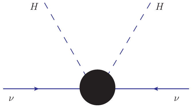
Figure 1: Neutrino effective mass.

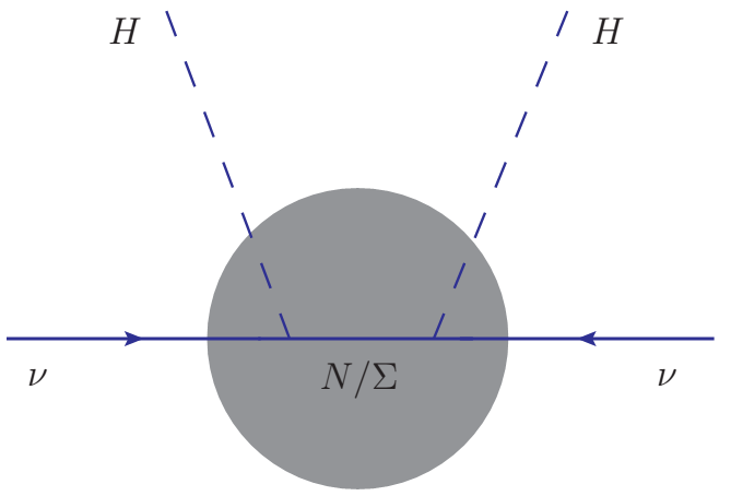
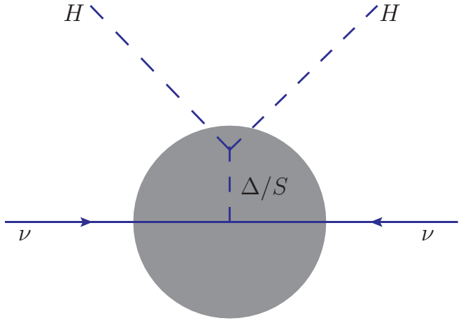
Figure 2: See-saw models.

When the fields transform under an additional symmetry group, such as an $A_{4}$ one, each of these (sub)processes itself will be further broken down to sub-sub-processes according to their symmetry structure. It is the spirit of the see-saw mechanism in a new scenario with an additionally introduced symmetry.

II.2 $A_{4}$-flavour symmetric see-saw models

There are also three types of see-saw models for this case corresponding to the above-described type I, II and III see-saw models (for some versions, see, for example, Barry:2010zk ; Felipe:2013vwa and references therein). Now, each of the processes in Fig. 2 becomes an effective process containing other (sub)processes. Let us consider an effective process, illustrated in Fig. 3, corresponding to the type I see-saw one, where $N$ is a fermion iso-singlet (or a set of fermion iso-singlets). This process in turn represents, accordingly to the rule (97f)–Appendix, a sum of different sub-processes (see Fig. 4 below). We will see this model in more details next section. The type III model (i.e., the model corresponding to the type III see-saw model) has a similar structure, where the fermion iso-singlets $N$’s are replaced by fermion iso-triplets $\Sigma$’s being also a triplet and singlets $1$, $1^{{}^{\prime}}$ and $1^{{}^{\prime\prime}}$ of $A_{4}$.

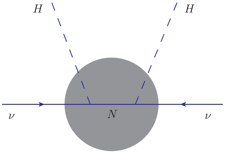
Figure 3: Type-I see-saw neutrino effective mass.

III $A_{4}$-flavour symmetric see-saw-I model

We present in this section an $A_{4}$-flavour symmetric extension of a type-I see-saw model, while the see-saw models of type-II and type-III can be investigated in separate works. There could be different versions of this extended model but the one given in Tab. 2 requires a minimal and “natural” extension, thus, this model can be referred to as the minimally extended model of the type-I see-saw model, or, just, the minimal model, for short.

	$\ell_{L}$	$\ell_{Ri}$	$\Phi_{h}$	$\Phi_{S}$	$\Phi_{S^{{}^{\prime}}}$	$\Phi_{S^{{}^{\prime\prime}}}$	$N_{T}$	$N_{S}$	$N_{S^{\prime}}$	$N_{S^{\prime\prime}}$
Spin	1/2	1/2	0	0	0	0	1/2	1/2	1/2	1/2
$SU(2)_{L}$	2	1, 1, 1	2	1	1	1	1	1	1	1
$A_{4}$	3	$1,1^{{}^{\prime}},1^{{}^{\prime\prime}}$	3	1	$1^{{}^{\prime}}$	$1^{{}^{\prime\prime}}$	3	1	$1^{{}^{\prime}}$	$1^{{}^{\prime\prime}}$

Table 2: An $A_{4}$-flavour symmetric extended standard model

The group transformation nature of the fields in the considered model is shown on the table, where $\ell_{L}=(\ell_{L1},\ell_{L2},\ell_{L3})$ and $\ell_{Ri}$, $i=1,2,3$, are the three generations of the left-handed- and the right-handed charged leptons, respectively. The three iso-doublets $\ell_{Li}$ form together an $A_{4}$-triplet, while the iso-singlets $\ell_{Ri}$ are also $A_{4}$-singlets, 1, $1^{\prime}$ and $1^{\prime\prime}$ (we can consider another version in which $\ell_{Ri}$ are components of an $A_{4}$-triplet). We note that the states $\ell_{i}$ ($\ell_{Li}$ and $\ell_{Ri}$) in general may not coincide with the states $l=e,\mu,\tau$, to which we need to make a rotation given in the subsection following. The new fermions $N_{T}$, $N_{S}$, $N_{S^{\prime}}$ and $N_{S^{\prime\prime}}$, being neutral fields and iso-singlets, are an $A_{4}$-triplet and three $A_{4}$-singlets 1, $1^{\prime}$ and $1"$, respectively.

The scalar field

$$\Phi_{h}^{T}=(\phi_{h1},\phi_{h2},\phi_{h3}),$$ (12)

is an $A_{4}$-triplet composed of three SM-like Higgs fields $\phi_{hi}$ being iso-doublets,

$$\phi_{hi}=\left(\begin{array}[]{c}\varphi_{i}^{+}\\[5.69054pt] \varphi_{i}^{0}\end{array}\right),~{}~{}i=1,2,3.$$ (13)

The vacuum expectation value (composed of those of the neutral components) of the scalar field $\Phi^{0}_{h}$ is denoted as

$$\langle\Phi^{0}_{h}\rangle^{T}=\left(\langle\varphi_{1}^{0}\rangle,\langle\varphi_{2}^{0}\rangle,\langle\varphi_{3}^{0}\rangle\right):={1\over\sqrt{2}}(v_{1},v_{2},v_{3}).$$ (14)

The structure of this vacuum expectation value (VEV), as well as the VEV’s of other scalar fields, can be fixed when the potential of the scalar sector is considered. The fields $\Phi_{S}$, $\Phi_{S^{{}^{\prime}}}$ and $\Phi_{S^{{}^{\prime\prime}}}$ are iso-singlet and $A_{4}$-singlet scalars with

$$\langle\Phi_{S}\rangle=\sigma_{1},~{}~{}\langle\Phi_{S^{{}^{\prime}}}\rangle=\sigma_{2},~{}~{}\langle\Phi_{S^{{}^{\prime\prime}}}\rangle=\sigma_{3},$$ (15)

denoting their VEV’s. These scalar fields can be re-expressed in terms of quantum fields $h_{i}$, $\eta_{i}$ and $\xi_{i}$ with zero VEV’s by shifting

$$\phi_{h1}=\left(\begin{array}[]{c}\varphi_{1}^{+}\\[5.69054pt] {1\over\sqrt{2}}(v_{1}+h_{1}+i\eta_{1})\end{array}\right),\hskip 8.5359pt\phi_{h2}=\left(\begin{array}[]{c}\varphi_{2}^{+}\\[5.69054pt] {1\over\sqrt{2}}(v_{2}+h_{2}+i\eta_{2})\end{array}\right),\hskip 8.5359pt\phi_{h3}=\left(\begin{array}[]{c}\varphi_{3}^{+}\\[5.69054pt] {1\over\sqrt{2}}(v_{3}+h_{3}+i\eta_{3})\end{array}\right),$$ (16)

and

$$\Phi_{S}=\sigma_{1}+\xi_{1},~{}~{}\Phi_{S^{\prime}}=\sigma_{2}+\xi_{2},~{}~{}\Phi_{S^{\prime\prime}}=\sigma_{3}+\xi_{3}.$$ (17)

Below, we shall choose to consider the type I see-saw model given in Tab. 2 and illustrated in Fig. 4.

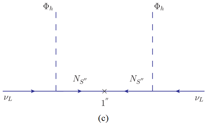
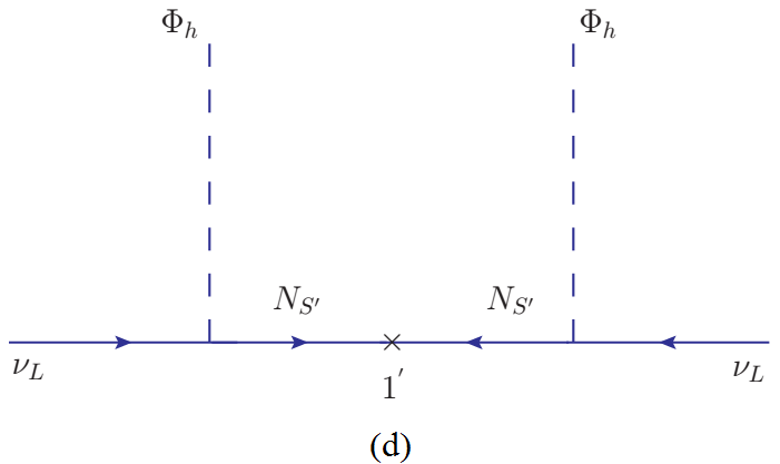
Figure 4: An $A_{4}$-flavour-symmetric type-I see-saw model.

Now, let us make a brief description of the scalar- and the lepton sector of the model (the quark sector not considered here requires a separate investigation).

III.1 Scalar sector

This sector consists of four scalars which are an iso-doublet $A_{4}$-triplet $\Phi_{h}$, and three iso-singlets $\Phi_{S}$, $\Phi_{S^{{}^{\prime}}}$ and $\Phi_{S^{{}^{\prime\prime}}}$ transforming as $A_{4}$-singlets 1, $1^{{}^{\prime}}$ and $1^{{}^{\prime\prime}}$, respectively. A logical model construction requires the symmetry breaking to follow this scheme:

$$\begin{array}[]{c}A_{4}\otimes SU(2)_{L}\otimes U(1)_{N}\\[5.69054pt] \downarrow\langle\mathcal{S}\rangle\\[5.69054pt] SU(2)_{L}\otimes U(1)_{Y}\\[5.69054pt] \downarrow\langle\Phi_{h}\rangle\\[5.69054pt] U(1)_{Q},\end{array}$$ (18)

where $\mathcal{S}$ stands for the scalars $\Phi_{S}$, $\Phi_{S^{{}^{\prime}}}$ and $\Phi_{S^{{}^{\prime\prime}}}$. The additional scalar fields may play a similar role as that of the scalar fields in a supersymmetric model Martin:1997ns in compensating divergences of fermion fields, therefore, we may not need SUSY in building a finite field theory (to have a precise conclusion we must make a detailed analysis which is beyond the subject of this paper).

Here, we briefly discuss the Higgs potential in the model. It has the general form

$$V=V(\Phi_{h})+V(\Phi_{h},\Phi_{S},\Phi_{S^{{}^{\prime}}},\Phi_{S^{{}^{\prime\prime}}})+V(\Phi_{S},\Phi_{S^{{}^{\prime}}},\Phi_{S^{{}^{\prime\prime}}}),$$ (19)

with

$$V(\Phi_{h})= ~{}\mu^{2}_{0}(\Phi_{h}^{\dagger}\Phi_{h})_{1}+\lambda_{1}(\Phi_{h}^{\dagger}\Phi_{h})^{2}_{1}+\lambda_{2}(\Phi_{h}^{\dagger}\Phi_{h})_{1^{{}^{\prime}}}(\Phi_{h}^{\dagger}\Phi_{h})_{1^{{}^{\prime\prime}}}$$

$$+\lambda_{3}(\Phi_{h}^{\dagger}\Phi_{h})_{3_{s}}(\Phi_{h}^{\dagger}\Phi_{h})_{3_{s}}+\lambda_{4}(\Phi_{h}^{\dagger}\Phi_{h})_{3_{a}}(\Phi_{h}^{\dagger}\Phi_{h})_{3_{a}}+\lambda_{5}(\Phi_{h}^{\dagger}\Phi_{h})_{3_{s}}(\Phi_{h}^{\dagger}\Phi_{h})_{3_{a}},$$ (20)

$$V(\Phi_{h},\Phi_{S},\Phi_{S^{{}^{\prime}}},\Phi_{S^{{}^{\prime\prime}}})= ~{}\gamma_{1}(\Phi_{h}^{\dagger}\Phi_{h})_{1}(\Phi_{S}^{\dagger}\Phi_{S})_{1}+\gamma_{2}(\Phi_{h}^{\dagger}\Phi_{h})_{1}(\Phi_{S^{\prime}}^{\dagger}\Phi_{S^{{}^{\prime\prime}}})_{1}$$

$$+\beta_{1}(\Phi_{h}^{\dagger}\Phi_{h})_{1^{{}^{\prime}}}(\Phi_{S^{\prime}}^{\dagger}\Phi_{S^{{}^{\prime}}})_{1^{{}^{\prime\prime}}}+\beta_{2}(\Phi_{h}^{\dagger}\Phi_{h})_{1^{{}^{\prime}}}(\Phi_{S^{\prime\prime}}^{\dagger}\Phi_{S})_{1^{{}^{\prime\prime}}}$$

$$+\eta_{1}(\Phi_{h}^{\dagger}\Phi_{h})_{1^{{}^{\prime\prime}}}(\Phi_{S^{\prime\prime}}^{\dagger}\Phi_{S^{{}^{\prime\prime}}})_{1^{{}^{\prime}}}+\eta_{2}(\Phi_{h}^{\dagger}\Phi_{h})_{1^{{}^{\prime\prime}}}(\Phi_{S^{\prime}}^{\dagger}\Phi_{S})_{1^{{}^{\prime}}}+H.c.,$$ (21)

$$V(\Phi_{S},\Phi_{S^{{}^{\prime}}},\Phi_{S^{{}^{\prime\prime}}})= ~{}\alpha_{0}(\Phi_{S}^{\dagger}\Phi_{S})_{1}+\alpha_{1}(\Phi_{S}^{\dagger}\Phi_{S})_{1}^{2}$$

$$+\alpha_{2}(\Phi_{S}^{\dagger}\Phi_{S})_{1}(\Phi_{S^{\prime}}^{\dagger}\Phi_{S^{{}^{\prime\prime}}})_{1}+\alpha_{3}(\Phi_{S^{\prime}}^{\dagger}\Phi_{S^{{}^{\prime\prime}}})_{1}$$

$$+\alpha_{4}(\Phi_{S^{\prime}}^{\dagger}\Phi_{S^{{}^{\prime\prime}}})_{1}(\Phi_{S^{\prime}}^{\dagger}\Phi_{S^{{}^{\prime\prime}}})_{1}+\alpha_{5}(\Phi_{S^{\prime}}^{\dagger}\Phi_{S^{{}^{\prime}}})_{1^{{}^{\prime\prime}}}(\Phi_{S^{\prime\prime}}^{\dagger}\Phi_{S^{{}^{\prime\prime}}})_{1^{{}^{\prime}}}+H.c..$$ (22)

For a logical reason, we require that $A_{4}$ symmetry should be broken at an energy scale higher (or much higher) than the electroweak one. This symmerty breaking can be caused when some or all of the scalar fields $\Phi_{S}$, $\Phi_{S^{{}^{\prime}}}$ and $\Phi_{S^{{}^{\prime\prime}}}$ acquire non-zero VEV’s. Therefore, $\Phi_{S}$, $\Phi_{S^{{}^{\prime}}}$ and $\Phi_{S^{{}^{\prime\prime}}}$, which can be candidates for the dark matter, should be sterile scalars interacting very weakly, or not interacting at all, with the SM fields including $\Phi_{h}$. That means that the interaction (21) should be much smaller than the interaction (20). After an $A_{4}$ symmetry breaking, $\Phi_{h}$ is seen as a single SM Higgs scalar coupled to three fermion generations with different coupling coefficients leading to different masses of the fermions.

Imposing the extremum condition to $\Phi_{h}$,

$$\left.\frac{\partial V}{\partial\phi_{h_{i}}}\right|_{\langle\phi_{h_{i}}\rangle=v_{i}}=0,~{}~{}~{}~{}(i=1,2,3),$$ (23)

we get an equation system of their VEV’s

$$\begin{cases}\mu_{0}^{2}+2(\lambda_{1}+\lambda_{2})v_{1}^{2}+(2\lambda_{1}-\lambda_{2}+2\lambda_{4}+\lambda_{5})v_{2}^{2}+(2\lambda_{1}-\lambda_{2}+2\lambda_{3}+\lambda_{5})v_{3}^{2}=0,\\ \mu_{0}^{2}+2(\lambda_{1}+\lambda_{2})v_{2}^{2}+(2\lambda_{1}-\lambda_{2}+2\lambda_{3}+\lambda_{5})v_{1}^{2}+(2\lambda_{1}-\lambda_{2}+2\lambda_{4}+\lambda_{5})v_{3}^{2}=0,\\ \mu_{0}^{2}+2(\lambda_{1}+\lambda_{2})v_{3}^{2}+(2\lambda_{1}-\lambda_{2}+2\lambda_{3}+\lambda_{5})v_{2}^{2}+(2\lambda_{1}-\lambda_{2}+2\lambda_{4}+\lambda_{5})v_{1}^{2}=0.\end{cases}$$ (24)

The latter equation system for general coefficients (general $\lambda_{0}$ and $\lambda_{i}$’s), is equivalent to the constraints

$$v_{1}^{2}=v_{2}^{2}=v_{3}^{2}:=v^{2},$$ (25)

leading to eight different choices,

$$\pm v_{1}=\pm v_{2}=\pm v_{3}=\pm v,$$

of the VEV’s structure of $\Phi_{h}$, where

$$v^{2}=\frac{-\mu_{0}^{2}}{2(3\lambda_{1}+\lambda_{3}+\lambda_{4}+\lambda_{5})}~{}\cdot$$ (26)

Due to the couplings of $\Phi_{h}$ to the SM fields, in particular, the SM gauge bosons, the VEV $v$ can have a value at the electroweak scale as in the SM.

In general, the Higgs fields defined above are flavour states but not mass-eigen states. To get their mass-eigen states one must diagonal the Higgs mass matrix appearing squared in the mass term

$$V_{M}(\Phi)\sim{1\over 2}\left(\begin{array}[]{ccc}h_{1}&h_{2}&h_{3}\end{array}\right)M_{h}^{2}\left(\begin{array}[]{c}h_{1}\\ h_{2}\\ h_{3}\end{array}\right),$$ (27)

where

$$M_{h}^{2}=\left(\begin{array}[]{ccc}p&q&q\\ q&p&q\\ q&q&p\end{array}\right),$$ (28)

with

$$p= 2v^{2}(\lambda_{1}+\lambda_{2}+\lambda_{3}+\lambda_{4}),$$

$$q= v^{2}(2\lambda_{1}-\lambda_{2}+\lambda_{5}).$$

As (28) is a real symmetric matrix, its eigenvalues, therefore, the scalar masses, are always real. It is not difficult to see that the matrix

$$U_{H}=\left(\begin{array}[]{ccc}\sqrt{1\over 3}&-\sqrt{2\over 3}&0\\[5.69054pt] \sqrt{1\over 3}&\sqrt{1\over 6}&-\sqrt{1\over 2}\\[5.69054pt] \sqrt{1\over 3}&\sqrt{1\over 6}&\sqrt{1\over 2}\end{array}\right).$$ (29)

can rotate the (squared) mass matrix $M_{h}^{2}$ to the diagonal matrix

$$M_{H}^{2}=\left(\begin{array}[]{ccc}m^{2}_{H1}&0&0\\[11.38109pt] 0&m^{2}_{H2}&0\\[11.38109pt] 0&0&m^{2}_{H3}\end{array}\right),$$ (30)

where

$$m_{H_{1}}^{2}=p+2q= 2(3\lambda_{1}+\lambda_{3}+\lambda_{4}+\lambda_{5})v^{2}=-\mu_{0}^{2},$$ (31)

$$m_{H_{2}}^{2}=m_{H_{3}}^{2}= ~{}p-q=(3\lambda_{2}+2\lambda_{3}+2\lambda_{4}-\lambda_{5})v^{2}$$

$$= -\mu^{2}_{0}-3(2\lambda_{1}-\lambda_{2}+\lambda_{5})v^{2},$$ (32)

are masses of the Higgs mass-eigen states $H_{i}$ related to the flavour states $h_{i}$ via the rotation

$$\left(\begin{array}[]{c}h_{1}\\ h_{2}\\ h_{3}\end{array}\right)=U_{H}^{t}\left(\begin{array}[]{c}H_{1}\\ H_{2}\\ H_{3}\end{array}\right).$$ (33)

A similar analysis can be done for other scalar fields. A more detailed analysis on the scalar sector is very interesting but such as analysis, however, goes beyond the scope of this paper, and therefore, it will be a subject of a separate work.

III.2 Lepton sector

The lepton sector contains charged leptons and neutrinos. In the present model, the charged lepton masses can be generated by the Yukawa terms of the Lagrangian

$$-\mathcal{L}_{Y_{cl}}= ~{}y_{1}(\overline{\ell}_{L}\Phi_{h})\ell_{R1}+y_{2}(\overline{\ell}_{L}\Phi_{h})^{{}^{\prime\prime}}\ell_{R2}+y_{3}(\overline{\ell}_{L}\Phi_{h})^{{}^{\prime}}\ell_{R3}+h.c.$$ (34)

After an $A_{4}$ and gauge symmetry breaking, the above-given Yukawa terms become

$$-\mathcal{L}_{Y_{cl}}= y_{1}(v_{1}\overline{\ell}_{L1}+v_{2}\overline{\ell}_{L2}+v_{3}\overline{\ell}_{L3})\ell_{R1}$$

$$+y_{2}(v_{1}\overline{\ell}_{L1}+\omega v_{2}\overline{\ell}_{L2}+\omega^{2}v_{3}\overline{\ell}_{L3})\ell_{R2}$$

$$+y_{3}(\overline{v_{1}\ell}_{L1}+\omega^{2}v_{2}\overline{\ell}_{L2}+\omega v_{3}\overline{\ell}_{L3})\ell_{R3}+h.c.,$$ (35)

and the charged leptons gain masses with the mass matrix

$$M_{lept}=\left(\begin{array}[]{ccc}y_{1}v_{1}&y_{2}v_{1}&y_{3}v_{1}\\ y_{1}v_{2}&\omega y_{2}v_{2}&\omega^{2}y_{3}v_{2}\\ y_{1}v_{3}&\omega^{2}y_{2}v_{3}&\omega y_{3}v_{3}\end{array}\right).$$ (36)

Taking into account (25), we can, without loss of generality, assume that $\langle\Phi_{h}\rangle^{T}=\frac{1}{\sqrt{2}}(v,v,v)$. The charged lepton mass matrix, then, takes the form

$$M_{lept}=\frac{1}{\sqrt{2}}U_{L}\left(\begin{array}[]{ccc}m_{e}&0&0\\ 0&m_{\mu}&0\\ 0&0&m_{\tau}\end{array}\right),$$ (37)

where

$$m_{e}=y_{1}v,~{}~{}m_{\mu}=y_{2}v,~{}~{}m_{\tau}=y_{3}v,$$ (38)

are the charged lepton masses, and

$$U_{L}=\frac{1}{\sqrt{3}}\left(\begin{array}[]{ccc}1&1&1\\ 1&\omega&\omega^{2}\\ 1&\omega^{2}&\omega\end{array}\right).$$ (39)

For the neutrinos, their masses can be generated by Yukawa terms of Dirac and Majorana type. First, we deal with the Dirac Yukawa terms

$$-\mathcal{L}_{Y_{\nu}}^{D}= ~{}y^{\nu}_{Ta}\left(\bar{\ell_{L}}\widetilde{\Phi}_{h}\right)_{3_{a}}\cdot N_{T}+y^{\nu}_{Tb}\left(\bar{\ell_{L}}\widetilde{\Phi}_{h}\right)_{3_{s}}\cdot N_{T}$$ (40)

$$+y^{\nu}_{S}\left(\bar{\ell_{L}}\widetilde{\Phi}_{h}\right)_{1}\cdot N_{S}+y^{\nu}_{S^{\prime}}\left(\bar{\ell_{L}}\widetilde{\Phi}_{h}\right)_{1^{\prime\prime}}\cdot N_{S^{\prime}}$$

$$+y^{\nu}_{S^{\prime\prime}}\left(\bar{\ell_{L}}\widetilde{\Phi}_{h}\right)_{1^{\prime}}\cdot N_{S^{\prime\prime}}+h.c..$$

The Dirac mass matrix extracted from these Yukawa terms is

$$M_{D}=\left(\begin{array}[]{ccccccccc}0&{y_{Ta}^{\nu}}v_{3}&{y_{Tb}^{\nu}}v_{2}&{y_{S}^{\nu}}v_{1}&{y_{S^{\prime}}^{\nu}}v_{1}&{y_{S^{\prime\prime}}^{\nu}}v_{1}\\ {y_{Tb}^{\nu}}v_{3}&0&{y_{Ta}^{\nu}}v_{1}&{y_{S}^{\nu}}v_{2}&{y_{S^{\prime}}^{\nu}}v_{2}\omega^{2}&{y_{S^{\prime\prime}}^{\nu}}v_{2}\omega\\ {y_{Ta}^{\nu}}v_{2}&{y_{Tb}^{\nu}}v_{1}&0&{y_{S}^{\nu}}v_{3}&{y_{S^{\prime}}^{\nu}}v_{3}\omega&{y_{S^{\prime\prime}}^{\nu}}v_{3}\omega^{2}\end{array}\right).$$ (41)

The Majorana Yukawa terms have the form

$$-\mathcal{L}_{Y_{\nu}}^{M}= ~{}y_{T_{1}}^{M}\left(\overline{N}_{T}N_{T}\right)_{1}\Phi_{S}+y_{T_{2}}^{M}\left(\overline{N}_{T}N_{T}\right)_{1^{{}^{\prime}}}\Phi_{S^{{}^{\prime\prime}}}+y_{T_{2}}^{M}\left(\overline{N}_{T}N_{T}\right)_{1^{{}^{\prime\prime}}}\Phi_{S^{{}^{\prime}}}$$

$$+y_{1}^{M}\left(\overline{N}_{S}N_{S}\right)_{1}\Phi_{S}+y_{2}^{M}\left(\overline{N}_{S^{{}^{\prime}}}N_{S^{{}^{\prime\prime}}}\right)_{1}\Phi_{S}$$

$$+y_{3}^{M}\left(\overline{N}_{S^{{}^{\prime}}}N_{S^{{}^{\prime}}}\right)_{1^{{}^{\prime\prime}}}\Phi_{S^{{}^{\prime}}}+y_{4}^{M}\left(\overline{N}_{S}N_{S^{{}^{\prime\prime}}}\right)_{1^{{}^{\prime\prime}}}\Phi_{S^{{}^{\prime}}}$$

$$+y_{5}^{M}\left(\overline{N}_{S^{{}^{\prime\prime}}}N_{S^{{}^{\prime\prime}}}\right)_{1^{{}^{\prime}}}\Phi_{S^{{}^{\prime\prime}}}+y_{6}^{M}\left(\overline{N}_{S}N_{S^{{}^{\prime}}}\right)_{1^{{}^{\prime}}}\Phi_{S^{{}^{\prime\prime}}}+h.c..$$ (42)

The latter Lagrangian (III.2) can be re-witten as

$$-\mathcal{L}_{Y_{\nu}}^{M}=\frac{1}{2}\overline{(N_{R})^{c}}\cdot M_{R}\cdot N_{R}+h.c.,$$ (43)

where

$$N_{T}= \left(N_{T1},N_{T2},N_{T3}\right)^{T},$$ (44)

$$N_{R}= \left(N_{T1},N_{T2},N_{T3},N_{S},N_{S^{\prime}},N_{S^{\prime\prime}}\right)^{T},$$ (45)

and

$$M_{R}=\left(\begin{array}[]{ccccccccc}M_{11}&0&0&0&0&0\\ 0&M_{22}&0&0&0&0\\ 0&0&M_{33}&0&0&0\\ 0&0&0&M_{44}&M_{45}&M_{46}\\ 0&0&0&M_{54}&M_{55}&M_{56}\\ 0&0&0&M_{64}&M_{65}&M_{66}\\ \end{array}\right)$$ (46)

is the Majorana mass matrix in the present case with

$$M_{11} =y_{T_{1}}^{M}\sigma_{1}+~{}~{}~{}y_{T_{2}}^{M}\sigma_{2}+~{}~{}~{}y_{T_{3}}^{M}\sigma_{3},$$

$$M_{22} =y_{T_{1}}^{M}\sigma_{1}+\omega^{2}y_{T_{2}}^{M}\sigma_{2}+\omega~{}y_{T_{3}}^{M}\sigma_{3},$$

$$M_{33} =y_{T_{1}}^{M}\sigma_{1}+\omega~{}y_{T_{2}}^{M}\sigma_{2}+\omega^{2}y_{T_{3}}^{M}\sigma_{3},$$

$$M_{44} =y_{1}^{M}\sigma_{1},~{}~{}~{}M_{56}=M_{65}=y_{2}^{M}\sigma_{1},$$

$$M_{55} =y_{3}^{M}\sigma_{2},~{}~{}~{}M_{46}=M_{64}=y_{4}^{M}\sigma_{2},$$

$$M_{66} =y_{5}^{M}\sigma_{3},~{}~{}~{}M_{45}=M_{54}=y_{6}^{M}\sigma_{3}.$$ (47)

It is not easy to diagonalize the Majorana mass matrix (46) in its general form which, however, is not always physical. Therefore, we could make some assumptions which are physically reasonable and can simlify the diagonalization of the mass matrix (46).

We assume that interactions between the sterile neutrinos and each of the sterile scalars have strengths of the same order, that is,

• $y_{1}^{M}=y_{2}^{M}$, that means $M_{44}=M_{56}=M_{65}$,

• $y_{3}^{M}=y_{4}^{M}$, that means $M_{55}=M_{46}=M_{64}$,

• $y_{5}^{M}=y_{6}^{M}$, that means $M_{66}=M_{45}=M_{54}$.

Thus the Majorana mass takes now the form

$$M_{R}=\left(\begin{array}[]{ccccccccc}M_{11}&0&0&0&0&0\\ 0&M_{22}&0&0&0&0\\ 0&0&M_{33}&0&0&0\\ 0&0&0&M_{44}&M_{66}&M_{55}\\ 0&0&0&M_{66}&M_{55}&M_{44}\\ 0&0&0&M_{55}&M_{44}&M_{66}\\ \end{array}\right).$$ (48)

Taking into account (40) and (III.2) we write the Yukawa terms for neutrinos

$$\mathcal{L}_{Y_{\nu}}=\mathcal{L}_{Y_{\nu}}^{D}+\mathcal{L}_{Y_{\nu}}^{M}$$ (49)

as follows

$$\mathcal{L}_{Y_{\nu}}=\frac{1}{2}\overline{n}_{L}M_{\rm seesaw}(n_{L})^{c}+h.c,$$ (50)

where

$$n_{L}=\left(\nu_{L},(N_{R})^{c}\right)^{T},$$ (51)

and

$$M_{\rm seesaw}=\left(\begin{array}[]{cc}0&M_{D}\\ M_{D}^{T}&M_{R}\end{array}\right).$$ (52)

From here, we get the type-I see-saw mass matrix

$$M_{\nu}=-M_{D}^{T}(M_{R})^{-1}M_{D},$$ (53)

which in the charged-lepton diagonalizing basis becomes

$$\mathcal{M}_{\nu}=U_{L}^{\dagger}M_{\nu}U_{L}^{\ast}=\left(\begin{array}[]{ccc}A&B&C\\ B&E&D\\ C&D&F\end{array}\right),$$ (54)

Before finishing this section let us discuss the mass scales, $M_{R}$, $M_{D}$ and $M_{\nu}$, involved. The general ranges of these mass scales are given in Tab. 5. According to the current experimental data Olive:2016xmw the upper bound of the light neutrino masses (the scale of $M_{\nu}$) is below $10^{-1}$ eV = $10^{-10}$ GeV. Thus, if the scale of $M_{D}$ is known, we can estimate the mass scale $M_{R}$ in relation to the coupling coefficients in (40) and (III.2), and vice versa, knowing $M_{R}$ we can determine $M_{D}$. While the scale $M_{\nu}$ is bounded today narrowly between 0 eV and $10^{-1}$ eV (even less), the scales of $M_{R}$ and $M_{D}$ still vary in wider ranges covering the electroweak (EW) scale $10^{2}$ GeV as well as the LHC discovering potential at about 1 TeV = $10^{3}$ GeV. On searching for heavy Majorana neutrinos within the type-I see-saw mechanism with the ATLAS detector in $\sqrt{s}=8$ TeV $pp$ collisions Aad:2015xaa the range of $M_{R}$ has been set to be between 100 – 500 GeV, while the ranges given by CMS are 90 GeV $<M_{R}<200$ GeV (for $ee$ final states in $\sqrt{s}=7$ TeV $pp$ collisions) Chatrchyan:2012fla and 40 GeV $<M_{R}<500$ GeV (for $\mu\mu$ final states in $\sqrt{s}=8$ TeV $pp$ collisions) Khachatryan:2015gha . An $M_{R}$ at the GUT scale and an $M_{D}$ at the EW scale are often taken in a see-saw model (see, for example, Dinh:2006ia and references therein) but, in general, the range of $M_{R}$, as mentioned earlier, could spread from the eV scale to the GUT scale (see, for example, Adhikari:2016bei and references therein) and $M_{D}$, at least here, is not constrained yet by any other constraint besides that related to Yukawa coupling coefficients in (40) and (III.2). A determination or estimation of the latter (via measurements of some processes such as those involved charged leptons) can shed a light on the scale of $M_{D}$ and thus on that of $M_{R}$. The branching ratios of a charged lepton decay tells us that these Yukawa coupling coefficients could be at least four magnitudes (10^-4) below that of an EW one, hence $M_{D}$ could be at the order 10^-2 GeV at most, thus, $M_{R}$ could be at the 10 TeV scale at most. Interestingly, the recent observation of 3.5 keV X-ray signals from several galaxies and galaxy clusters Bulbul:2014sua ; Boyarsky:2014jta could be explained by a decay of keV sterile neutrinos. The latter, if in a see-saw model, lead to very small (unless the VEV of the related scalar field(s) is small or the scale of $M_{\nu}$ is big enough) Dirac mass scale and coupling coefficients (see Tab. 5), the measurement of which is still very difficult.

Mass scale	$\mathbf{M_{R}}$ (GeV)	$\mathbf{M_{\nu}}$ (GeV)	$\mathbf{M_{D}=(M_{\nu}M_{R})^{1/2}}$ (GeV)	$\mathbf{y_{D}=M_{D}v^{-1}}$
GUT	$\sim 10^{15}$	$<10^{-10}$	$\sim 10^{2}\div 10^{3}$	$\sim 10^{0}\div 10^{1}$
TeV	$\sim 10^{3}$	$<10^{-10}$	$\sim 10^{-4}\div 10^{-3}$	$\sim 10^{-6}\div 10^{-5}$
GeV	$\sim 10^{0}$	$<10^{-10}$	$\sim 10^{-5}$	$\sim 10^{-7}$
MeV	$\sim 10^{-3}$	$<10^{-10}$	$\sim 10^{-7}\div 10^{-6}$	$\sim 10^{-9}\div 10^{-8}$
keV	$\sim 10^{-6}$	$<10^{-10}$	$\sim 10^{-8}$	$\sim 10^{-10}$
eV	$\sim 10^{-9}$	$<10^{-10}$	$\sim 10^{-10}\div 10^{-9}$	$\sim 10^{-12}\div 10^{-11}$

Figure 5: Mass scales of the model.

IV Neutrino masses and mixing

It is observed from (40), (43) and (54) that if

$$y_{S}^{\nu}=y_{S^{{}^{\prime}}}^{\nu}=y_{S^{{}^{\prime\prime}}}^{\nu},~{}~{}~{}y_{Ta},y_{Tb}\ll y_{S}^{\nu},~{}~{}~{}M_{55}=M_{66},$$ (55)

the neutrino mass matrix having the form

$$\mathcal{M}_{\nu 0}=\frac{1}{\Lambda}\left(\begin{array}[]{ccc}3(M_{44}+M_{66})(y_{S}^{\nu})^{2}&-3M_{66}(y_{S}^{\nu})^{2}&-3M_{66}(y_{S}^{\nu})^{2}\\ -3M_{66}(y_{S}^{\nu})^{2}&-3M_{66}(y_{S}^{\nu})^{2}&3(M_{44}+M_{66})(y_{S}^{\nu})^{2}\\ -3M_{66}(y_{S}^{\nu})^{2}&3(M_{44}+M_{66})(y_{S}^{\nu})^{2}&-3M_{66}(y_{S}^{\nu})^{2}\end{array}\right),$$ (56)

where

$$\Lambda=(M_{44}-M_{66})(M_{44}+2M_{66}),$$ (57)

can be diagonalized

$${\rm diag}(\mathcal{M}_{\nu 0})={(U^{\prime}_{tbm})}^{T}\mathcal{M}_{\nu 0}U^{\prime}_{tbm},$$ (58)

by the matrix

$$U^{\prime}_{tbm}=\left(\begin{array}[]{ccc}\sqrt{\frac{2}{3}}&\sqrt{\frac{1}{3}}&0\\ -\sqrt{\frac{1}{6}}&\sqrt{\frac{1}{3}}&-\sqrt{\frac{1}{2}}\\ -\sqrt{\frac{1}{6}}&\sqrt{\frac{1}{3}}&\sqrt{\frac{1}{2}}\end{array}\right).$$ (59)

That means, the model with the condition (55) is a TBM model. Here, the matrix $U^{\prime}_{tbm}$ can be converted to a more convenient form

$$U_{tbm}=\left(\begin{array}[]{ccc}\sqrt{\frac{2}{3}}&\sqrt{\frac{1}{3}}&0\\ -\sqrt{\frac{1}{6}}&\sqrt{\frac{1}{3}}&\sqrt{\frac{1}{2}}\\ \sqrt{\frac{1}{6}}&-\sqrt{\frac{1}{3}}&\sqrt{\frac{1}{2}}\end{array}\right),$$ (60)

However, as said above (and also in Ky:2016rzl ; Dinh:2015tna ), the experimental PNMS mixing matrix has a small deviation from a TBM form, therefore, the former can be presented as a perturbation around the latter. It follows from the fact that the difference, say $\Delta U$, between the experimental PNMS mixing matrix Olive:2016xmw and the TBM one is just a small correction to the latter (upto a phase factor):

$$\Delta U=\left(\begin{array}[]{ccc}0.006&-0.029&0.153e^{-i\delta}\\ -0.008-0.084e^{i\delta}&0.047\,-0.056e^{i\delta}&-0.054\\ -0.041-0.095e^{i\delta}&0.027\,-0.064e^{i\delta}&0.034\\ \end{array}\right).$$ (61)

Therefore, the (actual) neutrino mass matrix diagonalisable by the (experimental) PMNS mixing matrix, can be developed pertubatively around the TBM one Ky:2016rzl ; Dinh:2015tna ; Brahmachari:2014npa . As the present model under the condition (55) becomes a TBM model, a realistic model can be obtained by imposing a condition slightly differing from (55). In other words, to obtain a realistic model we could replace (55) by another condition which at the first order of approximation reads

$$y_{S^{{}^{\prime}}}^{\nu}=y_{S}^{\nu}+\epsilon_{1},~{}~{}~{}y_{S^{{}^{\prime\prime}}}^{\nu}=y_{S}^{\nu}+\epsilon_{2},~{}~{}~{}M_{55}=M_{66}+\sigma,$$ (62)

with $\epsilon_{i}$, $i=1,2$, and $\sigma$ are small number (i.e., $|\epsilon_{i}|,|\sigma|\ll 1$). From here we can develope perturbation of the Dirac and the Majorana mass matrix $M_{D}$ and $M_{R}$ around their TBM limit $M_{D_{0}}$ and $M_{R_{0}}$ respectively,

$$M_{D}=M_{D_{0}}+\Delta_{D}$$ (63)

and

$$M_{R}^{-1}=M_{R_{0}}^{-1}+\Delta_{R},$$ (64)

where $\Delta_{D}$ and $\Delta_{R}$ are small corrections to $M_{D_{0}}$ and $M_{R_{0}}^{-1}$, respectively. Now the neutrino mass matrix has the following (perturbative) form

$$\mathcal{M}_{\nu}=(M_{D_{0}}+\Delta_{D})^{T}(M_{R_{0}}^{-1}+\Delta_{R})(M_{D_{0}}+\Delta_{D})$$ (65)

which can be re-written as

$$\mathcal{M}_{\nu}=\mathcal{M}_{\nu 0}+\mathcal{W},$$ (66)

where

$$\mathcal{M}_{\nu 0}=M_{D_{0}}^{T}M_{R_{0}}^{-1}M_{D_{0}},$$ (67)

is the TBM mass matrix (56) and ${\cal W}$ is a deviation from the latter

$${\cal W}=\frac{1}{\Lambda^{{}^{\prime}}}\left(\begin{array}[]{ccc}e_{1}&e_{2}&e_{2}^{\ast}\\ e_{2}&e_{4}&e_{3}\\ e_{2}^{\ast}&e_{3}&e_{4}^{\ast}\end{array}\right),$$ (68)

with

$$\Lambda^{{}^{\prime}}=\frac{2(M_{44}-M_{66})\left[(M_{44}-M_{66})(M_{44}+2M_{66})-3\sigma M_{66}\right]}{y_{S}^{\nu}}$$ (69)

and

$$e_{1}= -\frac{4(\epsilon_{1}+\epsilon_{2})(M_{44}-M_{66})\left[M_{66}(2M_{66}+\sigma)-(M_{44}+M_{66})(M_{44}-\sigma)\right]}{(M_{44}+2M_{66})}$$

$$+\frac{6y_{S}^{\nu}(M_{44}-M_{66})^{2}}{(M_{44}+2M_{66})},$$

$$e_{2}= ~{}(\epsilon_{1}+\epsilon_{2})(M_{66}-M_{44})(M_{66}+2M_{44})+3\sqrt{3}i(\epsilon_{1}-\epsilon_{2})M_{66}(M_{44}-M_{66})$$

$$+2\sigma(\epsilon_{1}-2\epsilon_{2})(\omega M_{44}-M_{66})-2\sqrt{3}i\sigma(2\epsilon_{1}-\epsilon_{2})M_{66},$$

$$e_{3}= -2(\epsilon_{1}+\epsilon_{2})(M_{44}-M_{66})(M_{44}+2M_{66})+2\sigma(\epsilon_{1}-2\epsilon_{2})M_{44}-2\sigma(\epsilon_{2}-5\epsilon_{1})M_{66},$$

$$e_{4}= ~{}2(M_{44}+2M_{66})\left[2(\epsilon_{1}+\epsilon_{2})(M_{44}-M_{66})-3\omega\sigma y_{S}^{\nu}\right]$$

$$+4\sigma(\epsilon_{1}+\epsilon_{2})(2\omega M_{66}-\omega^{2}M_{44}-3M_{66}).$$ (70)

The TBM mixing matrix can be expressed in terms of eigen-vectors $|n^{0}\rangle$, $n=1,2,3$, of $\mathcal{M}_{\nu 0}$ and also $\mathcal{M}_{\nu 0}^{\dagger}\mathcal{M}_{\nu 0}$ as follows

$$U_{TBM}=\left(|1^{0}\rangle,|2^{0}\rangle,|3^{0}\rangle\right).$$ (71)

The eigen-vectors $|n\rangle$ of the matrix $\mathcal{M}_{\nu}^{\dagger}\mathcal{M}_{\nu}$ perturbatively developed around $|n^{0}\rangle$ have the form (taken upto the first perturbation order)

$$|n\rangle=|n^{0}\rangle+\sum_{k\neq n}\lambda_{nk}|k^{0}\rangle+...,$$ (72)

where

$$\lambda_{nk}= (|m_{n}^{0}|^{2}-|m_{k}^{0}|^{2})^{-1}V_{nk},$$ (73)

$$V_{nk}= \langle n^{0}|\mathcal{M}_{\nu 0}^{\dagger}\mathcal{W}+\mathcal{W}^{\dagger}\mathcal{M}_{\nu 0}|k^{0}\rangle,$$ (74)

and $|m_{i}^{0}|^{2}$, $i=1,2,3$, are eigenvalues of $\mathcal{M}_{\nu 0}^{\dagger}\mathcal{M}_{\nu 0}$.

Now we can diagonalize the neutrino mass matrix square $\mathcal{M}_{\nu}^{\dagger}\mathcal{M}_{\nu}$,

$$\tilde{U}^{\dagger}\mathcal{M}_{\nu}^{\dagger}\mathcal{M}_{\nu}\tilde{U}=\text{diag}~{}(|m_{1}|^{2},|m_{2}|^{2},|m_{3}|^{2}),$$ (75)

by the matrix

$$\tilde{U}=\begin{matrix}\left(\begin{array}[]{llr}\sqrt{\frac{2}{3}}+\sqrt{\frac{1}{3}}x^{*}&\sqrt{\frac{1}{3}}-\sqrt{\frac{2}{3}}x&-\sqrt{\frac{2}{3}}y-\sqrt{\frac{1}{3}}z\\ -\sqrt{\frac{1}{6}}+\sqrt{\frac{1}{3}}x^{*}+\sqrt{\frac{1}{2}}y^{*}&\sqrt{\frac{1}{3}}+\sqrt{\frac{1}{6}}x+\sqrt{\frac{1}{2}}z^{*}&\sqrt{\frac{1}{2}}+\sqrt{\frac{1}{6}}y-\sqrt{\frac{1}{3}}z\\ \sqrt{\frac{1}{6}}-\sqrt{\frac{1}{3}}x^{*}+\sqrt{\frac{1}{2}}y^{*}&-\sqrt{\frac{1}{3}}-\sqrt{\frac{1}{6}}x+\sqrt{\frac{1}{2}}z^{*}&\sqrt{\frac{1}{2}}-\sqrt{\frac{1}{6}}y+\sqrt{\frac{1}{3}}z\end{array}\right),\end{matrix}$$ (76)

with

$$x=\lambda_{12},\hskip 5.69046pty=\lambda_{13},\hskip 5.69046ptz=\lambda_{23}.$$ (77)

Any matrix $U^{\prime}$, related to $\tilde{U}$ by the relation $U^{\prime}=\tilde{U}\times P^{\prime}$, where $P^{\prime}={\rm diag}\left(e^{i\alpha^{\prime}_{1}/2},e^{i\alpha^{\prime}_{2}/2},e^{i\alpha^{\prime}_{3}/2}\right),$ with arbitrary $\alpha^{\prime}_{1}$, $\alpha^{\prime}_{2}$, $\alpha^{\prime}_{3}$, is also able to diagonalize $\mathcal{M}_{\nu}^{\dagger}\mathcal{M}_{\nu}$. Therefore, a PMNS matrix $U_{PMNS}$ can be defined upto a phase matrix $P^{\prime}$,

$$U_{PMNS}=\tilde{U}\times P^{\prime},$$ (78)

Writing $P^{\prime}$ as $P^{\prime}=e^{i\alpha^{\prime}_{3}/2}{\rm diag}\left(e^{i(\alpha^{\prime}_{1}-\alpha^{\prime}_{3})/2},e^{i(\alpha^{\prime}_{2}-\alpha_{3})/2},1\right)\equiv e^{i\alpha^{\prime}_{3}/2}{\rm diag}\left(e^{i{\alpha^{\prime}}_{21}/2},e^{i{\alpha^{\prime}}_{31}/2},1\right)$, we see that the phase $\alpha^{\prime}_{3}$ can be removed by redefining the overall field phase as done in the case of $P$. Thus, one can write $P^{\prime}$ in a form similar to that of $P$ in (2):

$$P^{\prime}={\rm diag}\left(e^{i{\alpha^{\prime}}_{21}/2},e^{i{\alpha^{\prime}}_{31}/2},1\right).$$ (79)

It is important to mention that $x$, $y$ and $z$, in general, are complex numbers, so do the matrix elements of $\tilde{U}$, therefore, not only the mixing angles but also the Majorana phases can get a small correction from $\tilde{U}$. The latter, through complex $x$, $y$ and $z$, has six degrees of freedom (DOF’s). Four of them parametrize the three mixing angles and the CPV phase. The other two DOF’s, namely, two phases, can be used to synchronize the phases of $P^{\prime}$ with those of $P$. Therefore, two of $x$, $y$ and $z$ (or two of their independent linear combinations) can be taken to be real. Comparing (3) with (76), we see that it is reasonable to choose a real $x$.

Using the trivial properties of the PMNS matrix given in (3), $\tan^{2}\theta_{12}=|U_{12}|^{2}/|U_{11}|^{2}$, $\sin\theta_{13}=|U_{13}|$, $\tan^{2}\theta_{23}=|U_{23}|^{2}/|U_{33}|^{2}$, applied to (76), we obtain at the first perturbation order the following relations:

$$\tan^{2}\theta_{12}\approx\frac{1-2\sqrt{2}{\rm Re}(x)}{2+2\sqrt{2}{\rm Re}(x)},$$ (80)

$$\sin\theta_{13}=\left|\sqrt{\frac{2}{3}}y+\sqrt{\frac{1}{3}}z\right|,$$ (81)

$$\tan^{2}\theta_{23}\approx\frac{1+2\sqrt{2}{\rm Re}\left(\sqrt{\frac{1}{6}}y-\sqrt{\frac{1}{3}}z\right)}{1-2\sqrt{2}{\rm Re}\left(\sqrt{\frac{1}{6}}y-\sqrt{\frac{1}{3}}z\right)}.$$ (82)

Further, from Eqs. (1) and (78), it is easy to get

$$\begin{array}[]{c}\left(\sqrt{\frac{2}{3}}+\sqrt{\frac{1}{3}}x^{*}\right)e^{i\alpha^{\prime}_{21}/2}=c_{12}c_{13}e^{i\alpha_{21}/2},\\[8.53581pt] \left(\sqrt{\frac{1}{3}}-\sqrt{\frac{2}{3}}x\right)e^{i\alpha^{\prime}_{31}/2}=s_{12}c_{13}e^{i\alpha_{31}/2},\\[8.53581pt] \left(-\sqrt{\frac{2}{3}}y-\sqrt{\frac{1}{3}}z\right)=s_{13}e^{-i\delta}.\end{array}$$ (83)

In general, as $x$ is complex, $\alpha^{\prime}_{21}\neq\alpha_{21}$ and $\alpha^{\prime}_{31}\neq\alpha_{31}$, but in the case of a real $x$ we have (at the first order of perturbation) $\alpha^{\prime}_{21}=\alpha_{21}$ and $\alpha^{\prime}_{31}=\alpha_{31}$.

Below, to check how our model works we will consider the case of a real parameter $x$, that is $P^{\prime}=(e^{i\alpha_{21}/2},e^{i\alpha_{31}/2},1)=P$, as argued above. Now, the PMNS matrix (78) gets the form

$$U_{PMNS}=\begin{matrix}\left(\begin{array}[]{lll}\sqrt{\frac{2}{3}}+\sqrt{\frac{1}{3}}x&\sqrt{\frac{1}{3}}-\sqrt{\frac{2}{3}}x&-\sqrt{\frac{2}{3}}y-\sqrt{\frac{1}{3}}z\\ -\sqrt{\frac{1}{6}}+\sqrt{\frac{1}{3}}x+\sqrt{\frac{1}{2}}y^{*}&\sqrt{\frac{1}{3}}+\sqrt{\frac{1}{6}}x+\sqrt{\frac{1}{2}}z^{*}&\sqrt{\frac{1}{2}}+\sqrt{\frac{1}{6}}y-\sqrt{\frac{1}{3}}z\\ \sqrt{\frac{1}{6}}-\sqrt{\frac{1}{3}}x+\sqrt{\frac{1}{2}}y^{*}&-\sqrt{\frac{1}{3}}-\sqrt{\frac{1}{6}}x+\sqrt{\frac{1}{2}}z^{*}&\sqrt{\frac{1}{2}}-\sqrt{\frac{1}{6}}y+\sqrt{\frac{1}{3}}z\end{array}\right)\times P.\end{matrix}$$ (84)

Deriving $x$, $y$ and $z$ by matching the matrix elements $(U_{PMNS})_{11}$, $(U_{PMNS})_{13}$ and $(U_{PMNS})_{23}$ in Eq. (84) with the corresponding elements of the experimentally measured PMNS matrix at the current best fit value of neutrino oscillation data Olive:2016xmw ; Capozzi:2017ipn ; Esteban:2016qun , then, inserting them back in Eq. (84), we obtain the PMNS matrix given by the model

$$U_{PMNS}^{model}=\begin{matrix}\left(\begin{array}[]{lll}0.8221&0.5695&0.1530\,e^{-i\delta}\\ -0.4337-0.0883\,e^{i\delta}&0.6252-0.0624\,e^{i\delta}&0.6533\\ 0.3716-0.0883\,e^{i\delta}&-0.5373-0.0624\,e^{i\delta}&0.7609\end{array}\right)\times P.\end{matrix}$$ (85)

In the following, to check the present model we are going to analyze and discuss in the model scenario several physics quantities, which can be verified experimentally, such as the neutrinoless double beta decay effective mass $|\langle m_{ee}\rangle|$, CPV phase $\delta_{CP}\equiv\delta$ and Jarlskog parameter $J_{CP}$, using the PMNS matrix (76) matched with the current neutrino oscillation data Olive:2016xmw ; Capozzi:2017ipn ; Esteban:2016qun .

Neutrinoless double beta decay ($0\nu\beta\beta$) is a process of emitting two electrons from relevant nuclei without producing any (anti)neutrino, thus violating the lepton number by 2 units Elliott:2004hr ; Avignone:2007fu ; Rodejohann:2011mu ; Elliott:2002xe ; Bilenky:2002aw ; Bilenky:2012qi ; GomezCadenas:2011it ; Schwingenheuer:2012jt . The ($0\nu\beta\beta$) decay together with the radiative emission of neutrino pair (RENP) from atom Yoshimura:2011ri ; Dinh:2012qb ; Fukumi:2012rn are the only two, so far, proposed processes, used for construction of experiments for determination of the nature of neutrinos (if they are of Dirac- or Majorana type). With its importance in understanding neutrino properties, the phenomenon of the ($0\nu\beta\beta$) decay has attracted interest of and has been studied by a large number of physicists in both theoretical and experimental aspects. Presently, the most sensitive experiments give an upper bound on the ($0\nu\beta\beta$) decay effective mass to be about $|\langle m_{ee}\rangle|<0.2-0.6$ eV (Heidelberg-Moscow KlapdorKleingrothaus:2000sn ), or $0.3-0.71$ eV (COURICINO Andreotti:2010vj ), or $0.14-0.38$ eV (EXO-200 Auger:2012ar ), while the next generation of the experiments Bellini:2009zw ; Gornea:2011zz may obtain a signal of the decay if $|\langle m_{ee}\rangle|$ is not smaller than $(2-5)\times 10^{-2}$ eV. In the scenario of the present model, the ($0\nu\beta\beta$) decay effective mass has the form

$$|\langle m_{ee}\rangle|=\left|m_{1}U_{e1}^{2}+m_{2}U_{e2}^{2}e^{i\alpha_{21}}+m_{3}U_{e3}^{2}e^{i\alpha_{31}}\right|.$$ (86)

The dependence of $|\langle m_{ee}\rangle|$ on the PMNS mixing matrix and the lightest active neutrino mass $m_{0}$ is depicted in Fig. 6.

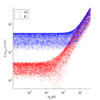
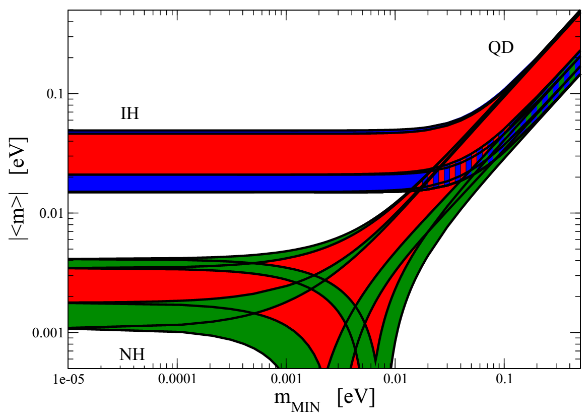
Figure 6: The ($0\nu\beta\beta$) effective mass $|\langle m_{ee}\rangle|$ as a function of the lightest neutrino mass. Left panel: Plot obtained by using (84) with neutrino mixing angles taken arbitrary in $3\sigma$ ranges, while the phases $\delta$, $\alpha_{21}$ and $\alpha_{31}$ varying in $[0,2\pi]$. Right panel: Plot taken from Olive:2016xmw .

To measure the Dirac CPV phase $\delta$ is a challenge but with the nonzero value of $\theta_{13}$ obtained by recent experiments, the measurement of $\delta$ becomes more realistic. The simplest and direct strategy, which has been arranged experimentally, is to determine the difference between the probabilities of a neutrino transition and an anti-neutrino transition Barger:1980jm ; Pakvasa:1980bz ,

$$A_{CP}^{(\alpha,\beta)}= P(\nu_{\alpha}\rightarrow\nu_{\beta})-P(\bar{\alpha}_{\alpha}\rightarrow\bar{\nu}_{\beta})$$

$$= -16J_{\alpha\beta}\sin\Delta_{12}\sin\Delta_{23}\sin\Delta_{31},$$ (87)

where $\Delta_{ij}\equiv\Delta m^{2}_{ij}L/4E$, and $J_{\alpha\beta}$ is the Jarlskog invariant quantity Jarlskog:1985ht ,

$$J_{\alpha\beta}=J_{CP}={\rm Im}\{U_{\alpha 1}^{*}U_{\beta 2}^{*}U_{\alpha 1}U_{\beta 2}\}=J_{CP}^{max}\sin\delta.$$ (88)

Using the canonical parametrization of the PMNS matrix expressed in Eq. (3), it is not difficult to obtain

$$J_{CP}^{max}=\cos\theta_{12}\sin\theta_{12}\cos\theta_{23}\sin\theta_{23}\cos^{2}\theta_{13}\sin\theta_{13}.$$ (89)

For the value of $\theta_{13}$ obtained by recent experiments, $J_{CP}^{max}$ takes value in the interval $[0.032-0.042]$ with neutrino oscillation angles varying in $3\sigma$ allowed ranges (learn more in Fig. 7). We see that the most possible values of $\delta$ are located around $\pi$/2 (=90^∘) and $3\pi$/2 (=270^∘), where $|J_{CP}|$ would take a value, which in fact is the maximal value $J_{CP}^{max}$, between $0.032-0.042$.

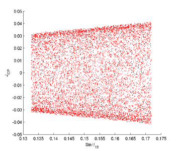
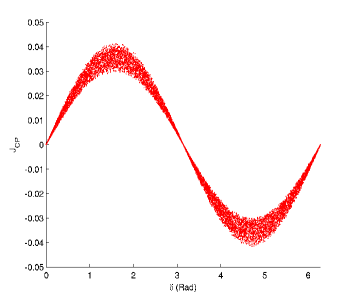
Figure 7: $J_{CP}$ as a function of $\theta_{13}$ (left panel) and $\delta_{CP}$ (right panel) with neutrino mixing angles taken in $3\sigma$ allowed ranges, and the CPV phase varying in $[0,2\pi]$.

When $x$ is real, it is easy to see from Eqs. (80)–(82), the value of the mixing angle $\theta_{12}$ depends only on $x$, while the other two mixing angles $\theta_{13}$ and $\theta_{23}$ as well as the Dirac CPV phase $\delta$ are determined by $y$ and $z$ via, for example, the equations

$$\sin\theta_{13}e^{-i\delta}= -\sqrt{\frac{2}{3}}y-\sqrt{\frac{1}{3}}z,$$ (90)

$$\tan^{2}\theta_{23}= \frac{1+2\sqrt{2}{\rm Re}\left(\sqrt{\frac{1}{6}}y-\sqrt{\frac{1}{3}}z\right)}{1-2\sqrt{2}{\rm Re}\left(\sqrt{\frac{1}{6}}y-\sqrt{\frac{1}{3}}z\right)}.$$ (91)

Since $y$ and $z$ are complex numbers, they contain four parameters. One of these parameters can be used to synchronize a Majorana phase (as mentioned above), two are used to fix the mixing angles $\theta_{13}$ and $\theta_{23}$, and the remaining one is used for the Dirac CPV phase $\delta$. Therefore, $\delta$ can theoretically take any value in the range of $[0,2\pi]$.

Let us consider some specific values of parameters $x$, $y$, for example $y=0$ or $z=0$. In case $y=0$ and $z$ arbitrary (or $z=0$ and $y$ arbitrary), we have only two free parameters to fix 3 measurements $\theta_{13}$, $\theta_{23}$ and $\delta$, thus $\delta$ can be expressed in term of $\theta_{13}$, $\theta_{23}$. For $y=0$, we have

$$-\sqrt{\frac{1}{3}}z= \sin\theta_{13}e^{-i\delta},$$ (92)

$$\tan^{2}\theta_{23}= \frac{1+2\sqrt{2}{\rm Re}\left(-\sqrt{\frac{1}{3}}z\right)}{1-2\sqrt{2}{\rm Re}\left(-\sqrt{\frac{1}{3}}z\right)}.$$ (93)

Eliminating $z$ in Eqs. (92), we obtain the constraint

$$\sin\theta_{13}\cos\delta=\frac{1}{2\sqrt{2}}\frac{\tan^{2}\theta_{23}-1}{\tan^{2}\theta_{23}+1}.$$ (94)

We can find $\delta$ from (94) for a given set of the mixing angles (see their experimental data in Tab. 1). If a value $\delta_{0}$ is a solution of (94) so is $2\pi-\delta_{0}$, therefore, it is enough to discuss one of them. This constraint gives, for example, at the best fit value (BFV) of the mixing angles $\theta_{13}$ and $\theta_{23}$ in an NO (and similarly for an IO), $\cos\delta=-0.291$, corresponding to the value $\delta\approx 4.414$ (and also $\delta\approx 1.866$). In general, this value of $\delta$ is not its mean value (BFV) but can give a rough estimation of the latter.

Based on the constraint (94), the distributions of $\delta$ for a normal ordering (NO) and an inverse ordering (IO), are depicted in Fig. 8, followed by Fig. 9, where $\delta$ as function of $\theta_{13}$ is plotted also for both cases. For each of these distributions generated by 10000 events, the Dirac CPV phase $\delta$, and, thus, the Jarlskog parameter $J_{CP}$ (plotted in Figs. 10 and 11), is numerically calculated event by event with an input ($s_{ij}$) taken randomly on the base of a Gaussian distribution characterized by an experimental mean value (best fit value) and sigmas given in Tab. 1. These distributions $\delta$ have a mean values $\bar{\delta}_{NO}=4.417\approx 1.41\pi$ (for an NO) and $\bar{\delta}_{IO}=4.616\approx 1.47\pi$ (for an IO) which are close to the global fits at $\delta=\delta_{NO}\equiv 1.39\pi$ and at $\delta=\delta_{IO}\equiv 1.31\pi$, respectively Olive:2016xmw ; Capozzi:2017ipn ; Esteban:2016qun .

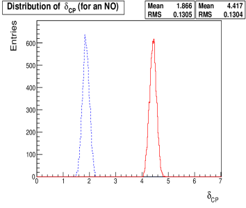
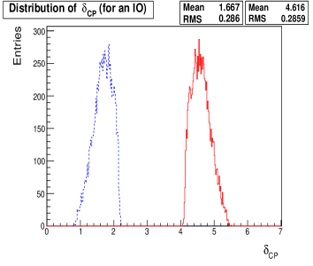
Figure 8: Distributions of $\delta_{CP}$ in an NO and an IO for two solutions distinguished by red and blue.

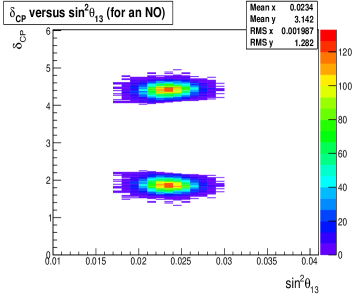
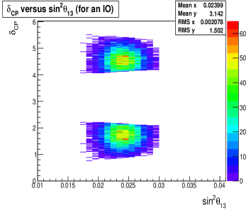
Figure 9: $\delta_{CP}$ as a function of $\theta_{13}$ in an NO and an IO, where the 1$\sigma$, 2$\sigma$ and 3$\sigma$ regions are colored in red, green and blue, respectively.

Using (88) and (89), the distributions of $J_{CP}$ corresponding to those of $\delta$ in two cases of hierarchy are depicted in Figs. 10 and 11. Because of the symmetry of $J_{CP}$ only its positive part is plotted in Fig. 10. The values of $J_{CP}$ obtained around 0.032 (for an NO) and 0.034 (for an IO) are quite consistent with the ones given in Olive:2016xmw .

Figure 10: Distribution of $J_{CP}$ in an NO and an IO

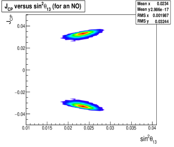
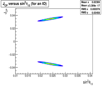
Figure 11: $J_{CP}$ as a function of $\theta_{13}$ in an NO and an IO.

To summarise, we note that the best fit values of $\delta$ and $J_{CP}$ obtained here are very close (in general, at the $1\sigma$ region) to the global fit given in Olive:2016xmw ; Capozzi:2017ipn ; Esteban:2016qun .

V Conclusions

We stress again that neutrino masses and mixing are an experimental fact. Neutrinos are massive but their masses are very tiny. Therefore, an actual problem is to find a way to explain the smallness of the neutrino masses and the see-saw mechanism is one of the most popular ways serving this purpose. So far many models of neutrino masses and mixing including those with the flavour symmetry have been proposed. In particular, the models based on the discrete group $A_{4}$ has attracted much interest and has been investigated quite intensively for the last several years. A natural question arising is whether and how the see-saw mechanism can be extended to the case of a flavour symmetric SM. The see-saw mechanism has been applied by other authors to separate sub-processes (classified by an $A_{4}$ symmetry), but, to our knowledge, no universal and systematic formulation of the see-saw mechanism has been made for an $A_{4}$-flavour symmetric SM yet. In the present paper such a formulation with an accent on a type-I see-saw model has been made. So, an ordinary see-saw process is treated as an effective process suming up all possible sub-processes corresponding to irreducible representations of the $A_{4}$ group.

The scalar sector of the latter model contains an $A_{4}$-triplet $\Phi_{h}$ of iso-doublet scalars and three $A_{4}$-singlet iso-singlet scalars $\Phi_{S}$, $\Phi_{S}^{{}^{\prime}}$ and $\Phi_{S}^{{}^{\prime\prime}}$. In our scheme, these $A_{4}$-singlets when acquiring a VEV, violate the extended symmetry down to the SM one, the $A_{4}$-triplet would play the role of the SM Higgs. The real parts of the three neutral components of $\Phi_{h}$ are super-positions of three mass-eigen states, one of which could be the SM Higgs. A detailed analysis on the scalar sector is a subject of a separate work.

The lepton sector of the above-mentioned model consists of the SM-like leptons transforming now under also the group $A_{4}$ as its three- or one-dimensional representations, and four new iso-singlet fields transforming as an $A_{4}$-triplet and three $A_{4}$-singlets $1$, $1^{\prime}$ and $1^{\prime\prime}$. These newly introduced iso-singlet fields, referred to as right-handed neutrinos, are necessary for the neutrino mass generation via the type-I see-saw mechanism. Applying a perturbation method to this model we obtain a neutrino mass and mixing structure from where several important quantities, such as neutrinoless double beta decay effective mass $|\langle m_{ee}\rangle|$, CP violation phase $\delta_{CP}$ and Jarlskog parameter $J_{CP}$ are predicted. The predicted values of these quantities within the present model fit quite well to the current experimental data Olive:2016xmw . After finishing this work we have learned that our results are consistent to the results announced recently by the T2K collaboration Iwamoto:2016yth , in particular, the values of $\delta_{CP}$ obtained by us, in both the NO and the IO, are very close to those announced by the T2K.

For conclusion, it is shown once again in this paper the usefulness of the see-saw mechanism applied to $A_{4}$ flavour symmetric standard models predicting new particles, interesting relations and values of some physics quantities which can be tested experimentally. Compared with our previous work Ky:2016rzl , the advantage of the present approach is that no introduction of an additional symmetry $Z_{3}\times Z_{4}$ is needed. An illustration has been done within a type-I (see-saw) model, but it can be also done with other-type models, or with all-type models.

Appendix A Representations of $A_{4}$ in brief

Being a group of all even permutations of four objects, $A_{4}$ has 12 elements, which can be divided into 4 conjugate classes, thus is also an order 4 group Ishimori:2010au ; Altarelli:2010gt ; Altarelli:2009kr . Geometrically, it is also called the tetrahedral group describing the orientation-preserving symmetry of a regular tetrahedron. The elements of $A_{4}$ can be generated by two basic generators $S$ and $T$ satisfying the relations

$$S^{2}=T^{3}=(ST)^{3}=1.$$ (95)

This group has four unitary representations, including three one-dimensional representations $1,~{}1^{\prime},~{}1^{\prime\prime}$ and one three-dimensional representation generated via $S$ and $T$ as follows:

$$1:\hskip 5.69046ptS=1,\hskip 8.5359ptT=1,$$ (96a)

$$1^{{}^{\prime}}:\hskip 5.69046ptS=1,\hskip 8.5359ptT=e^{i2\pi/3}\equiv\omega,$$ (96b)

$$1^{{}^{\prime\prime}}:\hskip 5.69046ptS=1,\hskip 8.5359ptT=e^{i4\pi/3}\equiv\omega^{2},$$ (96c)

$$3:\hskip 5.69046ptS=\left(\begin{array}[]{ccc}1&0&0\\ 0&-1&0\\ 0&0&-1\end{array}\right),\hskip 8.5359ptT=\left(\begin{array}[]{ccc}0&1&0\\ 0&0&1\\ 1&0&0\end{array}\right).$$ (96d)

Usually, applications of representations of a group require us to know the decomposition rule of a tensor product between irreducible representations into irreducible representations. This rule in the case of $A_{4}$ reads

$$1\times 1=1,$$ (97a)

$$1^{{}^{\prime}}\times 1^{{}^{\prime\prime}}=1,$$ (97b)

$$1^{{}^{\prime\prime}}\times 1^{{}^{\prime}}=1,$$ (97c)

$$1^{{}^{\prime}}\times 1^{{}^{\prime}}=1^{{}^{\prime\prime}},$$ (97d)

$$1^{{}^{\prime\prime}}\times 1^{{}^{\prime\prime}}=1^{{}^{\prime}},$$ (97e)

$$3\times 3=1+1^{{}^{\prime}}+1^{{}^{\prime\prime}}+3_{a}+3_{s}.$$ (97f)

The first five rules are trivial but the last one needs more explanation. For two triplets $3_{A}\sim(a_{1},a_{2},a_{3})$ and $3_{B}\sim(b_{1},b_{2},b_{3})$, the irreducible components of their tensor product $3_{A}\times 3_{B}$ according to (97f) are

$$1=a_{1}b_{1}+a_{2}b_{2}+a_{3}b_{3},$$ (98a)

$$1^{{}^{\prime}}=a_{1}b_{1}+\omega^{2}a_{2}b_{2}+\omega a_{3}b_{3},$$ (98b)

$$1^{{}^{\prime\prime}}=a_{1}b_{1}+\omega a_{2}b_{2}+\omega^{2}a_{3}b_{3},$$ (98c)

$$3_{a}\sim(a_{2}b_{3},a_{3}b_{1},a_{1}b_{2}),$$ (98d)

$$3_{s}\sim(a_{3}b_{2},a_{1}b_{3},a_{2}b_{1}).$$ (98e)

The information of the $A_{4}$ representations given above is important for construction of a Lagrangian of a model adopting an $A_{4}$ flavour symmetry. Basing on the structure of tensor products of representations of $A_{4}$ we can build different see-saw models corresponding to this flavour symmetry.

References

- (1) D. J. Griffiths, “Introduction to elementary particles”, John Wiley Sons, New York, 1987.
- (2) T. P. Cheng and L.F. Li, “Gauge theory of elementary particle physics”, Oxford university press, Oxford, 2006.
- (3) M. E. Peskin and D. V. Schroeder, “An introduction to quantum field theory”, Addison-Wesley publishing company, Reading, Massachusetts, 1995.
- (4) Ho Kim Quang and Pham Xuan Yem, “Elementary particles and their interactions: concepts and phenomena”, Springer-Verlag, Berlin, 1998.
- (5) G. Aad et al. (ATLAS collaboration), Phys. Lett. B716 (2012)
- (6) S. Chatrchyan et al. (CMS collaboration), Phys. Lett. B716 (2012)
- (7) Nguyen Anh Ky and Nguyen Thi Hong Van, Commun. Phys. 25, 1 (2015) [arXiv:1503.08630 [hep-ph]].
- (8) Y. Fukuda et al. [Super-Kamiokande Collaboration], Phys. Lett. B 433, 9 (1998).
- (9) Y. Fukuda et al. [Super-Kamiokande collaboration], Phys. Lett. B 436, 33 (1998).
- (10) Y. Fukuda et al. [Super-Kamiokande collaboration], Phys. Rev. Lett. 81, 1562 (1998).
- (11) Q. R. Ahmad et al. [SNO Collaboration], Phys. Rev. Lett. 87, 071301 (2001).
- (12) Q. R. Ahmad et al. [SNO Collaboration], Phys. Rev. Lett. 89, 011301 (2002).
- (13) Q. R. Ahmad et al. [SNO Collaboration], Phys. Rev. Lett. 89, 011302 (2002).
- (14) C. Patrignani et al. [Particle Data Group], “Review of Particle Physics”, Chin. Phys. C 40, 100001 (2016).
- (15) F. Capozzi, E. Di Valentino, E. Lisi, A. Marrone, A. Melchiorri and A. Palazzo, Phys. Rev. D 95, 096014 (2017).
- (16) I. Esteban, M. C. Gonzalez-Garcia, M. Maltoni, I. Martinez-Soler and T. Schwetz, JHEP 1701, 087 (2017).
- (17) P. F. Harrison, D. H. Perkins and W. G. Scott, Phys. Lett. B 530, 167 (2002).
- (18) P. Minkowski, Phys. Lett. B 67, 412 (1977).
- (19) M. Gell-Mann, P. Ramond and R. Slansky, “Complex spinors and unified theories in Supergravity”, (Workshop proceedings, Stony Brook, 27-29 September 1979, eds. P. Van Nieuwenhuizen and D. Z. Freedman), North-Holland, Amsterdam (1979), p. 341
- (20) R. N. Mohapatra and G. Senjanovic, Phys. Rev. Lett. 44, 912 (1980).
- (21) J. Schechter and J. W. F. Valle, Phys. Rev. D 22, 2227 (1980).
- (22) J. Schechter and J. W. F. Valle, Phys. Rev. D 25 774 (1982).
- (23) S. Bilenky, Introduction to the physics of massive and mixed neutrinos, Springer, Berlin, 2010.
- (24) R. N. Mohapatra and P. B. Pal, “Massive neutrinos in physics and astrophysics”, World Sci. Lect. Notes Phys. 60, 1(1998), [World Sci. Lect. Notes Phys. 72, 1 (2004)].
- (25) D. O. Caldwell and R. N. Mohapatra, Phys. Rev. D 48, 3259 (1993).
- (26) S. T. Petcov and A. Y. Smirnov, Phys. Lett. B 322, 109 (1994).
- (27) S. F. King, A. Merle, S. Morisi, Y. Shimizu and M. Tanimoto, New J. Phys. 16, 045018 (2014).
- (28) H. Ishimori, T. Kobayashi, H. Ohki, Y. Shimizu, H. Okada and M. Tanimoto, Prog. Theor. Phys. Suppl. 183, 1 (2010).
- (29) G. Altarelli and F. Feruglio, Rev. Mod. Phys. 82, 2701 (2010).
- (30) E. Ma and G. Rajasekaran, Phys. Rev. D 64, 113012 (2001).
- (31) E. Ma, Mod. Phys. Lett. A 17, 289 (2002).
- (32) K. S. Babu, E. Ma and J. W. F. Valle, Phys. Lett. B 552, 207 (2003).
- (33) E. Ma, Phys. Rev. D 70, 031901 (2004).
- (34) G. Altarelli and D. Meloni, J. Phys. G 36, 085005 (2009).
- (35) K. M. Parattu and A. Wingerter, Phys. Rev. D 84, 013011 (2011).
- (36) S. F. King and C. Luhn, JHEP 1203, 036 (2012).
- (37) G. Altarelli, F. Feruglio, L. Merlo and E. Stamou, JHEP 1208, 021 (2012).
- (38) G. Altarelli, F. Feruglio and L. Merlo, Fortsch. Phys. 61, 507 (2013).
- (39) P. M. Ferreira, L. Lavoura and P. O. Ludl, Phys. Lett. B 726, 767 (2013).
- (40) J. Barry and W. Rodejohann, Phys. Rev. D 81, 093002 (2010), [Phys. Rev. D 81, 119901 (2010)].
- (41) Y. H. Ahn and S. K. Kang, Phys. Rev. D 86, 093003 (2012).
- (42) R. Gonzalez Felipe, H. Serodio and J. P. Silva, Phys. Rev. D 88, 015015 (2013).
- (43) A. E. Carcamo Hernandez, I. de Medeiros Varzielas, S. G. Kovalenko, H. Päs and I. Schmidt, Phys. Rev. D 88 (2013) 076014 [arXiv:1307.6499 [hep-ph]].
- (44) I. de Medeiros Varzielas, O. Fischer and V. Maurer, JHEP 1508, 080 (2015).
- (45) P. Q. Hung and T. Le, JHEP 1509, 001 (2015), [JHEP 1509, 134 (2015)].
- (46) Nguyen Anh Ky, Phi Quang Van and Nguyen Thi Hong Van, Phys. Rev. D 94, 095009 (2016).
- (47) S. J. Gates, M. T. Grisaru, M. Rocek and W. Siegel, Front. Phys. 58, 1 (1983).
- (48) M. T. Grisaru and D. Zanon, Nucl. Phys. B 252, 578 (1985).
- (49) A. Galperin, Nguyen Anh Ky and E. Sokatchev, Mod. Phys. Lett. A 2, 33 (1987).
- (50) Nguyen Anh Ky, Bulg. J. Phys. 15, 311 (1988).
- (51) M. Drewes, Int. J. Mod. Phys. E 22, 1330019 (2013).
- (52) Dinh Nguyen Dinh, Nguyen Anh Ky, Nguyen Thi Hong Van and Phi Quang Van, Phys. Rev. D 74, 077701 (2006).
- (53) Nguyen Anh Ky and Nguyen Thi Hong Van, Phys. Rev. D 72, 115017 (2005).
- (54) A. Merle, Int. J. Mod. Phys. D 22, 1330020 (2013).
- (55) M. Drewes et al., JCAP 1701, 025 (2017) [arXiv:1602.04816 [hep-ph]].
- (56) S. P. Martin, Adv. Ser. Direct. High Energy Phys. 21, 1 (2010), [Adv. Ser. Direct. High Energy Phys. 18, 1 (1998)].
- (57) G. Aad et al. [ATLAS Collaboration], JHEP 1507, 162 (2015).
- (58) S. Chatrchyan et al. [CMS Collaboration], Phys. Lett. B 717, 109 (2012).
- (59) V. Khachatryan et al. [CMS Collaboration], Phys. Lett. B 748, 144 (2015).
- (60) E. Bulbul, M. Markevitch, A. Foster, R. K. Smith, M. Loewenstein and S. W. Randall, Astrophys. J. 789, 13 (2014).
- (61) A. Boyarsky, O. Ruchayskiy, D. Iakubovskyi and J. Franse, Phys. Rev. Lett. 113, 251301 (2014).
- (62) Dinh Nguyen Dinh, Nguyen Anh Ky, Phi Quang Vn and Nguyen Thi Hng Vn, “A prediction of for a normal neutrino mass hierarchy in an extended standard model with an A4 flavour symmetry” (in Proceedings of the 2nd International workshop on theoretical and computational physics (IWTCP-2), Buon-Ma-Thuot, 28-31 July 2014), J. Phys. Conf. Ser. 627, no. 1, 012003 (2015).
- (63) B. Brahmachari and P. Roy, JHEP 1502, 135 (2015).
- (64) S. R. Elliott and J. Engel, J. Phys. G 30, R183 (2004).
- (65) F. T. Avignone, III, S. R. Elliott and J. Engel, Rev. Mod. Phys. 80, 481 (2008).
- (66) W. Rodejohann, Int. J. Mod. Phys. E 20, 1833 (2011).
- (67) S. R. Elliott and P. Vogel, Ann. Rev. Nucl. Part. Sci. 52, 115 (2002).
- (68) S. M. Bilenky, C. Giunti, J. A. Grifols and E. Masso, Phys. Rept. 379, 69 (2003).
- (69) S. M. Bilenky and C. Giunti, Mod. Phys. Lett. A 27, 1230015 (2012).
- (70) J. J. Gomez-Cadenas, J. Martin-Albo, M. Mezzetto, F. Monrabal and M. Sorel, Riv. Nuovo Cim. 35, 29 (2012).
- (71) B. Schwingenheuer, J. Phys. Conf. Ser. 375, 042007 (2012).
- (72) M. Yoshimura, Phys. Lett. B 699, 123 (2011).
- (73) Dinh Nguyen Dinh, S. T. Petcov, N. Sasao, M. Tanaka and M. Yoshimura, Phys. Lett. B 719, 154 (2013).
- (74) A. Fukumi, S. Kuma, Y. Miyamoto, K. Nakajima, I. Nakano, H. Nanjo, C. Ohae and N. Sasao et al., PTEP 2012, 04D002 (2012).
- (75) H. V. Klapdor-Kleingrothaus et al., Eur. Phys. J. A 12, 147 (2001).
- (76) E. Andreotti et al., Astropart. Phys. 34, 822 (2011).
- (77) M. Auger et al. [EXO-200 Collaboration], Phys. Rev. Lett. 109, 032505 (2012).
- (78) F. Bellini et al., Astropart. Phys. 33, 169 (2010).
- (79) R. Gornea [EXO-200 Collaboration], J. Phys. Conf. Ser. 309, 012003 (2011).
- (80) S. M. Bilenky and S. T. Petcov, Rev. Mod. Phys. 59, 671 (1987), [Rev. Mod. Phys. 61, 169 (1989)], [Rev. Mod. Phys. 60, 575 (1988)].
- (81) V. D. Barger, K. Whisnant and R. J. N. Phillips, Phys. Rev. Lett. 45, 2084 (1980).
- (82) S. Pakvasa, AIP Conf. Proc. 68, 1164 (1980).
- (83) C. Jarlskog, Phys. Rev. Lett. 55, 1039 (1985).
- (84) K. Iwamoto [T2K Collaboration], “Recent results from T2K and future prospects”, PoS ICHEP 2016, 517 (2016). See also http://t2k-experiment.org/2017/08/t2k-2017-cpv/ .