Nonaxisymmetric MHD instabilities of Chandrasekhar states in Taylor-Couette geometry

Abstract

We consider axially periodic Taylor-Couette geometry with insulating boundary conditions. The imposed basic states are so-called Chandrasekhar states, where the azimuthal flow $U_{\phi}$ and magnetic field $B_{\phi}$ have the same radial profiles. Mainly three particular profiles are considered: the Rayleigh limit, quasi-Keplerian, and solid-body rotation. In each case we begin by computing linear instability curves and their dependence on the magnetic Prandtl number $\rm{Pm}$. For the azimuthal wavenumber $m=1$ modes, the instability curves always scale with the Reynolds number and the Hartmann number. For sufficiently small $\rm{Pm}$ these modes therefore only become unstable for magnetic Mach numbers less than unity, and are thus not relevant for most astrophysical applications. However, modes with $m>1$ can behave very differently. For sufficiently flat profiles, they scale with the magnetic Reynolds number and the Lundquist number, thereby allowing instability also for the large magnetic Mach numbers of astrophysical objects. We further compute fully nonlinear, three-dimensional equilibration of these instabilities, and investigate how the energy is distributed among the azimuthal ($m$) and axial ($k$) wavenumbers. In comparison spectra become steeper for large $m$, reflecting the smoothing action of shear. On the other hand kinetic and magnetic energy spectra exhibit similar behavior: if several azimuthal modes are already linearly unstable they are relatively flat, but for the rigidly rotating case where $m=1$ is the only unstable mode they are so steep that neither Kolmogorov nor Iroshnikov-Kraichnan spectra fit the results. The total magnetic energy exceeds the kinetic energy only for large magnetic Reynolds numbers $\rm{Rm}>100$.

1 Introduction

According to the Rayleigh criterion, an ideal non-magnetic flow is stable against axisymmetric perturbations whenever the specific angular momentum increases outward. In the presence of an azimuthal magnetic field $B_{\phi}$, this result is modified as

$$\frac{1}{R^{3}}\frac{{\rm{d}}}{{\rm{d}}R}(R^{2}{\it\Omega})^{2}-\frac{R}{\mu_{0}\rho}\frac{{\rm{d}}}{{\rm{d}}R}\left(\frac{B_{\phi}}{R}\right)^{2}>0,$$ (1)

where ${\it\Omega}$ is the angular velocity, $\mu_{0}$ the permeability, $\rho$ the density, and $(R,\phi,z)$ are standard cylindrical coordinates. This criterion is both necessary and sufficient for stability against axisymmetric perturbations (Michael, 1954). All ideal flows can thus be destabilized by adding azimuthal magnetic fields with suitable profiles and magnitudes.

For nonaxisymmetric modes one has ${{\rm{d}}}/{{\rm{d}}R}(RB_{\phi}^{2})<0$ as the necessary and sufficient condition for stability of an ideal fluid at rest (Vandakurov, 1972; Tayler, 1973). Outwardly increasing fields are therefore unstable, with azimuthal wavenumber $m=1$ being the most unstable (Acheson, 1978). If a differential rotation profile is now added, the variety of instabilities that are available grows considerably. Even the current-free (within the fluid) $B_{\phi}\propto 1/R$ profile can become unstable, and can as well be destabilized by a rotation profile that by itself would be stable according to the Rayleigh criterion. We have called this phenomenon the Azimuthal MagnetoRotational Instability (AMRI, see Rüdiger et al. (2014)); following theoretical suggestions by Hollerbach et al. (2010), this mode has by now been observed in a laboratory experiment (Seilmayer et al., 2014).

This combination of a magnetic field $B_{\phi}\propto 1/R$ and a rotation profile ${\it\Omega}\propto 1/R^{2}$ (potential flow) exactly at the Rayleigh limit is an example of a particular class of basic states defined by Chandrasekhar (1956) to consist of

$$\boldsymbol{U}=\boldsymbol{U}_{\rm A},$$ (2)

or more generally,

$$\boldsymbol{U}=\rm{Mm}\ \boldsymbol{U}_{\rm A}.$$ (3)

That is, the radial profiles of $\boldsymbol{U}$ and $\boldsymbol{U}_{\rm A}=\boldsymbol{B}/\sqrt{\mu_{0}\rho}$ are required to be the same, but there may be a constant of proportionality between the two, denoted as the magnetic Mach number $\rm{Mm}$, the ratio of the fluid velocity $\boldsymbol{U}$ to the Alfvén velocity $\boldsymbol{U}_{\rm A}$ (Tataronis & Mond, 1987). The magnetic Mach number of astrophysical objects often exceeds unity. Galaxies have $\rm{Mm}$ between 1 and 10 (Elstner et al., 2014), for the solar tachocline with a magnetic field of 1 kG one obtains $\rm{Mm}\simeq 30$, and for typical white dwarfs and neutron stars $\rm{Mm}\simeq 1000$. (On the other hand, for magnetars with fields of $\sim 10^{14}$ G and a rotation period of $\sim$1 s, the magnetic Mach number is $\sim 0.1-1$.)

Chandrasekhar (1956) showed that all basic states satisfying (2) are stable in the absence of diffusive effects. However, these states can be destabilized if at least one of the molecular diffusivities $\nu$ (kinematic viscosity) or $\eta$ (magnetic diffusivity) is non-zero. We argued that the class of states which fulfill the condition (3) yield a set of diffusive instabilities with several properties in common (Rüdiger et al., 2015). While Rüdiger et al. (2015) concentrated on linear results for the modes $m=\pm 1$, this study extends this work towards higher $m$ and concentrates especially on nonlinear effects in the saturated state.

As a reminder, for the azimuthal modes $m=1$ the marginal stability curves in the $\rm{Re}$-$\rm{Ha}$ plane converge for small magnetic Prandtl numbers

$$\rm{Pm}=\frac{\nu}{\eta}.$$ (4)

As a consequence, for sufficiently small $\rm{Pm}$ instability only exists for $\rm{Mm}<1$, that is, for slow rotation. Rapidly rotating flows with $\rm{Mm}>1$ require large $\rm{Pm}$ to become unstable. Cosmic objects indeed often possess small magnetic Prandtl numbers (see Brandenburg & Subramanian (2005)). For turbulent systems such as stellar convection zones or galaxies, the magnetic Prandtl number must be replaced by its effective turbulence-induced values, which are much larger. In the upper part of the solar radiative core the molecular value is about $\rm{Pm}\simeq 0.065$ (Gough, 2003). For low-mass red giants, however, the inclusion of the radiative viscosity leads to $O(1)$ magnetic Prandtl numbers (Rüdiger et al., 2015). As many of these magnetized cosmical objects combine large magnetic Mach numbers with small magnetic Prandtl numbers, the astrophysical relevance of these Chandrasekhar states, including AMRI, might seem to be limited. However, these results to date considered only azimuthal wavenumbers $m=1$. We will see in this work that $m>1$ modes may behave quite differently, with sufficiently flat profiles allowing instability for large $\rm{Mm}$ even for small $\rm{Pm}$, and hence yielding astrophysically relevant results after all.

Finally, for the sake of completeness, let us return briefly to axisymmetric modes, and demonstrate that any states satisfying (3) are always stable to such $m=0$ modes, provided only that the rotation rate does not increase outward. Taking ${\it\Omega}\propto R^{-q}$ with non-negative $q$, Michael’s relation (1) yields

$$(2-q){\rm{Mm}}^{2}+q>0$$ (5)

as a sufficient condition for stability. Hence, all flows and fields of the Chandrasekhar type with $0\leq q\leq 2$ are stable against axisymmetric perturbations. Note that the limits $q=0$ and $q=2$ define the two stringent solutions for the time-independent rotation laws following from the equation of angular momentum transport. Following Herron & Soliman (2006) all rotation laws between two insulating cylinders under the presence of toroidal fields due to an axial current inside the inner cylinder are stable against axisymmetric perturbations. Hence, AMRI in Taylor-Couette flows is strictly nonaxisymmetric.

2 Equations

We are interested in the stability of the background field $\boldsymbol{B}=(0,B_{\phi}(R),0)$ and the flow $\boldsymbol{U}=(0,R{\it\Omega}(R),0)$. The perturbed state of the system is described by the field $\boldsymbol{b}$ and the flow $\boldsymbol{u}$. We will be interested in both linearized and fully nonlinear solutions to the governing equations. For the linearized equations all quantities may be expanded in modal form as ${\boldsymbol{b}}={\boldsymbol{b}}(R){\rm exp}(\sigma t+{\rm i}(kz+m\phi)),$ etc., with the axial and azimuthal wavenumbers $k$ and $m$ as ‘input’ parameters, and $\sigma$ as the (complex) eigenvalue. The linearized equations are then

$$\frac{\partial\boldsymbol{u}}{\partial t}+(\boldsymbol{U}\cdot\nabla)\boldsymbol{u}+(\boldsymbol{u}\cdot\nabla)\boldsymbol{U}=-\frac{1}{\rho}\nabla p+\nu\Delta\boldsymbol{u}+$$

$$+\frac{1}{\mu_{0}\rho}{\rm curl}\ \boldsymbol{b}\times\boldsymbol{B}+\frac{1}{\mu_{0}\rho}{\rm curl}\ \boldsymbol{B}\times\boldsymbol{b},$$ (6)

$$\frac{\partial\boldsymbol{b}}{\partial t}={\rm curl}(\boldsymbol{u}\times\boldsymbol{B})+{\rm curl}(\boldsymbol{U}\times\boldsymbol{b})+\eta\Delta\boldsymbol{b},$$ (7)

and ${\rm div}\ \boldsymbol{u}={\rm div}\ \boldsymbol{b}=0$. For the full nonlinear problem (6) contains the additional terms $(\boldsymbol{u}\cdot\nabla)\boldsymbol{u}$ on the left and $({\rm curl}\ \boldsymbol{b}\times\boldsymbol{b})/(\mu_{0}\rho)$ on the right, and (7) contains the additional term ${\rm curl}(\boldsymbol{u}\times\boldsymbol{b})$ on the right. The modal expansion above also no longer holds; the spatial structure is instead allowed to be fully three-dimensional, and the evolution in time is via time-stepping rather than an eigenvalue problem.

The stationary background solutions which fulfill the condition (3) are

$${\it\Omega}=a+\frac{b}{R^{2}},\ \ \ \ \ \ \ \ \ \ \ \ \ \ \ \ \ B_{\phi}=\frac{\sqrt{\mu_{0}\rho}}{\rm{Mm}}\ (aR+\frac{b}{R}),$$ (8)

where $a$ and $b$ are constants defined by

$$a={\it\Omega}_{\rm{in}}\frac{\mu-r_{\rm in}^{2}}{1-{r_{\rm in}^{2}}},\qquad b={\it\Omega}_{\rm{in}}R_{\rm{in}}^{2}\frac{1-\mu}{1-{r_{\rm in}^{2}}},$$ (9)

with

$$r_{\rm in}=\frac{R_{\rm{in}}}{R_{\rm{out}}},\;\;\;\ \ \ \ \ \ \ \mu=\frac{{\it\Omega}_{\rm{out}}}{{\it\Omega}_{\rm{in}}}.$$ (10)

$R_{\rm{in}}$ and $R_{\rm{out}}$ are the radii of the inner and outer cylinders, and ${\it\Omega}_{\rm{in}}$ and ${\it\Omega}_{\rm{out}}$ are their rotation rates. A magnetic field of the form $b/R$ is generated by running an axial current only through the inner region $R<R_{\rm{in}}$, whereas a field of the form $aR$ is generated by running a uniform axial current through the entire region $R<R_{\rm{out}}$, including the fluid.

The toroidal field amplitude is usually measured by the Hartmann number

$$\rm{Ha}=\frac{B_{\rm in}R_{0}}{\sqrt{\mu_{0}\rho\nu\eta}}$$ (11)

of the azimuthal field $B_{\rm{in}}$ at the inner cylinder. $R_{0}=\sqrt{R_{\rm in}(R_{\rm out}-R_{\rm in})}$ is used as the unit of length, $\eta/R_{0}$ as the unit of velocity and $B_{\rm in}$ as the unit of the azimuthal fields. Frequencies, including the rotation ${\it\Omega}$, are normalized with the inner rotation rate ${\it\Omega}_{\rm in}$. The Reynolds numbers $\rm{Re}$ and $\rm{Rm}$ are defined by

$$\rm{Re}=\frac{{\it\Omega}_{\rm in}R_{0}^{2}}{\nu},\ \ \ \ \ \ \ \ \ \ \ \ \ \ {\rm{Rm}}=\frac{{\it\Omega}_{\rm in}R_{0}^{2}}{\eta},$$ (12)

and the magnetic Mach number is then related via

$$\rm{Mm}=\frac{\sqrt{\rm{Re}\rm{Rm}}}{\rm{Ha}}=\frac{\rm{Rm}}{\rm{S}}$$ (13)

with the Lundquist number $\rm{S}=\rm{Ha}\cdot\sqrt{\rm{Pm}}$ of the magnetic field.

The boundary conditions imposed at $R_{\rm{in}}$ and $R_{\rm{out}}$ are no-slip for $\boldsymbol{u}$ and insulating for $\boldsymbol{b}$. This translates to

$$u_{R}=u_{\phi}=u_{z}=0$$ (14)

at both boundaries,

$$b_{R}+{{\rm i}b_{z}\over I_{m}(kR)}\left({m\over kR}I_{m}(kR)+I_{m+1}(kR)\right)=0$$ (15)

at $R_{\rm in}$, and

$$b_{R}+{{\rm i}b_{z}\over K_{m}(kR)}\left({m\over kR}K_{m}(kR)-K_{m+1}(kR)\right)=0$$ (16)

at $R_{\rm out}$, where $I_{m}$ and $K_{m}$ are the modified Bessel functions. A more detailed derivation of the boundary conditions can be found in Rüdiger et al. (2013).

We fixed the radius ratio at $r_{\rm in}=0.5$. For the rotation ratio we then consider primarily the three values $\mu=0.25$, $1$ and $0.35$. The choice $\mu=0.25$ corresponds to a flow that is exactly at the Rayleigh limit ${\it\Omega}\propto 1/R^{2}$, and a field that is current-free within the fluid; any instabilities are therefore pure AMRI. The choice $\mu=1$ corresponds to a solid-body rotation, and a uniform electric current flowing throughout the entire region (what is known as a ‘pinch’ configuration in plasma physics). Any instabilities in this case are purely current-driven, what are also known as Tayler instabilities (TI). We will find that $m=1$ are the only instabilities in this case. The choice $\mu=0.35$ has aspects in common with both the AMRI and TI; that is, instabilities in this case can derive their energy from either the background flow $\boldsymbol{U}$ (AMRI) or the background field $\boldsymbol{B}$ (TI). The reason for the particular choice $\mu=0.35$ is that this represents the so-called quasi-Keplerian value where ${\it\Omega}\approx R^{-3/2}$, although according to (8) the profile is not exactly Keplerian, but merely has the values of $a$ and $b$ that fit a Keplerian ratio at the endpoints. Finally, a few calculations were also done at $\mu=0.5$, which corresponds to a so-called quasi-galactic profile, where $a$ and $b$ are fitted to ${\it\Omega}\approx R^{-1}$.

The linearized one-dimensional eigenvalue problem is solved using the numerical code described by Rüdiger et al. (2013), as well as further references therein. The nonlinear three-dimensional time-stepping problem is solved using the MPI-parallelized code described by Guseva et al. (2015), which itself is based on an earlier pipe flow solver by A.P. Willis (www.openpipeflow.org). The spatial structures in $z$ and $\phi$ are via Fourier modes $\exp(ikz+im\phi)$, allowing energy spectra in these two directions to be easily constructed. The periodic domain length in the axial direction is chosen as 10 times the gap width, to allow sufficient large structures to develop in $z$. Usually close to the linear onset of the instability the wavenumbers in axial direction conform to the gap width, thus they are well-captured. In axial direction between 64 and 256 Fourier modes have been used, in azimuthal between 32 and 128. For the radial direction the order of Chebyshev polynomials was varied between 127 and 511. In summary, the lowest resolution has been $127\times 64\times 32$, the highest $511\times 256\times 128$, depending mainly on the magnetic Reynolds number.

In the next section we use the linear code to investigate the onset of instabilities for our chosen values of $\mu$; in the section after that we use the nonlinear code to study their equilibration in the supercritical regime.

3 Linear Onset

We wish to compute the linear onset curves for the three azimuthal wavenumbers $m=1,\ 2,\ 3$, and the values $\mu=0.25$, 1, and 0.35 (plus a few results at 0.5). That is, for each choice of input parameters $\rm{Ha}$, $\rm{Re}$ and $\rm{Pm}$, we repeatedly solve the linear eigenvalue problem for a range of $k$, and find the value that yields the largest growth/decay rate, ${\rm Re}(\sigma)$. The curve where ${\rm Re}(\sigma)=0$ is then the linear onset curve, and we are particularly interested in how this curve scales as $\rm{Pm}\to 0$. Are the relevant parameters $\rm{Ha}$ and $\rm{Re}$, or $\rm{S}$ and $\rm{Rm}$, and does this perhaps differ for different values of $m$ and $\mu$?

3.1 The Rayleigh limit, $\boldsymbol{\mu=0.25}$

Figure 1: The stability maps for $\mu=0.25$ for $m=1,2,3$ and $\rm{Pm}=1$ (left), $\rm{Pm}=10^{-2}$ (middle) and $\rm{Pm}=10^{-4}$ (right). The dashed lines define $\rm{Mm}=1$. For $\rm{Pm}\to 0$ all curves satisfy the condition $\rm{Mm}<1$.

The value $\mu=0.25$ has a particular significance for both the flow and the field. For $\boldsymbol{U}$, it denotes the transition point from hydrodynamic instability for $\mu<0.25$ to stability for $\mu>0.25$, according to the Rayleigh criterion regarding the angular momentum $R^{2}{\it\Omega}$. For $\boldsymbol{B}$ we have that the associated electric currents flow only in the inner region $R<R_{\rm in}$. Any resulting instabilities are therefore purely magnetorotational in nature, not current-driven. As a result, no instabilities can occur for $\rm{Re}=0$; $\rm{Ha}=0$ is also excluded, as $\mu=0.25$ is already on the Rayleigh line where purely non-magnetic instabilities no longer exist.

Fig. 1 shows results for $\rm{Pm}=1$ to $\rm{Pm}=10^{-4}$. For all $m$, the curves have a characteristic shape consisting of lower and upper branches that each have positive slopes. That is, for a sufficiently large $\rm{Ha}$ to allow instability at all, it only exists within a finite range $\rm{Re}_{l}\leq\rm{Re}\leq\rm{Re}_{u}$, and vice versa when interchanging the roles of $\rm{Ha}$ and $\rm{Re}$. The global minimum values of $\rm{Re}$ and $\rm{Ha}$ are plotted in Fig. 2. Figs. 1 and 2 clearly reveal that: (i) The modes $m=2$ and 3 are also unstable, but $m=1$ is always the most unstable; (ii) Decreasing $\rm{Pm}$ pushes the onset to higher values of $\rm{Re}$ and $\rm{Ha}$, and more strongly for $m=2$ and 3 than for $m=1$; (iii) For sufficiently small $\rm{Pm}$ the critical parameters for all three azimuthal modes are $\rm{Re}$ and $\rm{Ha}$. This last result in particular means that as $\rm{Pm}\to 0$ all of the onset curves shift increasingly into the regime $\rm{Mm}<1$, making them astrophysically not relevant. On the other hand, it is precisely this feature that the scalings are $\rm{Re}$ and $\rm{Ha}$ rather than $\rm{Rm}$ and $\rm{S}$ that made these modes experimentally accessible (Hollerbach et al., 2010; Seilmayer et al., 2014).

Figure 2: The coordinates $\rm{Re}$ (top) and $\rm{Ha}$ (bottom) for the minima of the lines of marginal instability given in Fig. 1. For small $\rm{Pm}$ the lines for all $m$ scale with $\rm{Re}$ and $\rm{Ha}$.

3.2 Rigidly-rotating pinch, $\boldsymbol{\mu=1}$

The value $\mu=1$ also has special significance for both the flow and the field. For $\boldsymbol{B}$ it implies a uniform current throughout the entire region $R<R_{\rm out}$, what is known in plasma physics as a pinch configuration. For $\boldsymbol{U}$, it corresponds to solid-body rotation, with no differential rotation at all. Any resulting instabilities are therefore purely current-driven, with $\boldsymbol{U}$ not available as a source of energy. As a result, instabilities can occur for $\rm{Re}=0$ (corresponding to a stationary container), but not for $\rm{Ha}=0$.

Fig. 3 shows results for $\rm{Pm}=1$ to $\rm{Pm}=10^{-6}$. All curves start at $\rm{Ha}=28.1$ for $\rm{Re}=0$, then curve toward the right for $\rm{Re}>0$. That is, solid-body rotation has a stabilizing influence, which is strongest for $\rm{Pm}=1$ (Pitts & Tayler, 1985). Note also that only $m=1$ is unstable in this case. For $\rm{Re}=0$ this was previously known (Tayler, 1957); we here extend this result to $\rm{Re}>0$. The other key message from Fig. 3 is that once again, for sufficiently small $\rm{Pm}$ the critical parameters are $\rm{Re}$ and $\rm{Ha}$, so $\rm{Mm}<1$. And again, it is precisely this feature that is experimentally so convenient (Rüdiger et al., 2007; Rüdiger & Schultz, 2010; Seilmayer et al., 2012).

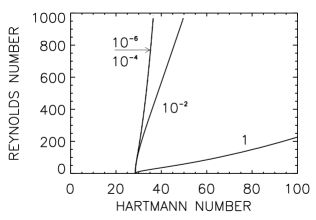
Figure 3: The stability maps for $\mu=1$, $m=1$ (the only unstable mode), and $\rm{Pm}$ as indicated next to each curve. Note how the curves become identical for $\rm{Pm}\leq 10^{-4}$.

3.3 Quasi-Keplerian rotation, $\boldsymbol{\mu=0.35}$

The previous results at $\mu=0.25$ and $1$ have been particularly simple, in the sense that any instabilities are necessarily either pure AMRI or pure TI, based simply on the energy source that is driving the instability. Any values in between, including the astrophysically relevant quasi-Keplerian profile $\mu=0.35$, or also the quasi-galactic $\mu=0.5$, are potentially far more complicated, as both $\boldsymbol{U}$ and $\boldsymbol{B}$ can act as energy sources. Not surprisingly then, the results are also more complicated than either of the ‘pure’ cases.

Figure 4: The stability maps for $\mu=0.35$ for $m=1,2,3$ and $\rm{Pm}=1$ (left), $\rm{Pm}=10^{-2}$ (middle) and $\rm{Pm}=10^{-4}$ (right). The dashed lines define $\rm{Mm}=1$. For $\rm{Pm}\to 0$ only the $m=1$ curve satisfies the condition $\rm{Mm}<1$.

Figs. 4 and 5 show the equivalents of Figs. 1 and 2. While there are some similarities, there are also many differences. Most importantly, as seen in Fig. 5, it is only for $m=1$ that the critical parameters are $\rm{Re}$ and $\rm{Ha}$. For $m=2,3$ the instabilities instead scale with $\rm{Rm}$ and $\rm{S}$. These new scalings as $\rm{Pm}\to 0$ suggest that these instabilities may have astrophysical applications, where $\rm{Pm}<1$ and $\rm{Mm}>1$ are often both satisfied. Because of their scaling with $\rm{Rm}$ and $\rm{S}$ these $m=2,3$ modes should also exist for vanishing viscosity, $\nu=0$. They cannot be reproduced, therefore, with codes based on the inductionless approximation ($\rm{Pm}=0$).

Figure 5: The coordinates $\rm{Rm}$ (left) and $\rm{S}$ (right) for the minima of the lines of marginal instability given in Fig. 4. For small $\rm{Pm}$ the lines for $m=1$ scale with $\rm{Re}$ and $\rm{Ha}$, but for $m=2,3$ they scale with $\rm{Rm}$ and $\rm{S}$. The dashed lines are for the quasi-galactic rotation profile $\mu=0.5$, and indicate that this behaves much the same as $\mu=0.35$.

4 Kinetic and magnetic energies

The kinetic and magnetic energies of magnetohydrodynamic turbulence are often assumed to be equipartitioned. To probe this idea the ratio

$$\varepsilon=\frac{\langle\boldsymbol{b}^{2}\rangle}{\mu_{0}\rho\langle\boldsymbol{u}^{2}\rangle}$$ (17)

of the two energies is calculated, averaged over the container. The stationary background solutions (8) are excluded.

In the top panels of Fig. 6 this ratio is plotted for various Reynolds numbers as a function of the magnetic Prandtl number. The Hartmann number is fixed, and $\mu$ takes the two values 0.25 and 0.35. The result is that for small magnetic Prandtl number ($\rm{Pm}\lesssim 10^{-2}$) the relation $\varepsilon\propto\rm{Pm}$ seems to hold, which implies that $\eta\langle\boldsymbol{b}^{2}\rangle/\mu_{0}\rho\simeq\nu\langle{\boldsymbol{u}}^{2}\rangle$, or equivalently $b_{\rm rms}=$O$(\sqrt{\rm{Pm}}u_{\rm rms})$. This dependence is weaker than that used by Roberts (1964), who suggested that for small $\rm{Pm}$ $b_{\rm rms}=$O$({\rm{Pm}}u_{\rm rms})$. For the given Reynolds numbers up to 50000, and magnetic Prandtl numbers smaller than a critical value of (say) 0.01, the instability pattern is always dominated by the kinetic fluctuations. However, the critical $\rm{Pm}$ depends on the applied Reynolds number; it becomes smaller for increasing $\rm{Re}$, and is evidently not the most appropriate measure to decide whether the state is magnetically or kinetically dominated.

The plot also shows that the influence of the global Reynolds number on this relation is only weak. For faster rotation the ratio (17) is somewhat larger than for slower rotation. For forced MHD turbulence models (Brandenburg, 2014) found a similar behavior for the viscous and ohmic dissipation, but for such models the magnetic energy reservoir is only filled by the work of the Lorentz force against the driven velocity field.

Figure 6: The ratio $\varepsilon=E_{\rm mag}/E_{\rm kin}$ between magnetic and kinetic energy as a function of $\rm{Pm}$ (top) and $\rm{Rm}$ (bottom) for $\mu=0.25$ (left, with $\rm{Ha}=600$) and $\mu=0.35$ (right, with $\rm{Ha}=1000$). $\varepsilon$ exceeds unity for $\rm{Rm}\simeq 200$. $\rm{Pm}$ is not an appropriate measure, but $\rm{Rm}$ is.

In the bottom panels of Fig. 6 the ratio $\varepsilon$ is plotted now as a function of the magnetic Reynolds number $\rm{Rm}$. One finds a clear scaling of the curves with $\rm{Rm}$ for both the potential rotation law $\mu=0.25$ as well as the quasi-Keplerian law $\mu=0.35$. The magnetic energy exceeds the kinetic energy for all $\rm{Rm}\gtrsim 200$. This behavior does not depend on the electric current associated with the basic state (8). For smaller magnetic Reynolds numbers the MHD instability is always dominated by the fluid motions. For larger $\rm{Rm}$ the energy ratio seems to become constant, in agreement with Rüdiger et al. (2014). Calculations with $\rm{Rm}<200$ are only weakly magnetized, while for larger $\rm{Rm}$ the pattern is magnetically dominated. If the curves do scale with $\rm{Rm}$ rather than $\rm{Pm}$, then fluids with $\rm{Pm}\ll 1$ will also become magnetically dominated once $\rm{Re}$ and $\rm{Rm}$ are sufficiently large, which is indeed the case for many astrophysical applications. This would not be possible if they scaled with $\rm{Pm}$. Experiments with liquid metals as the fluid between the cylinders will always lead to $\varepsilon<1$ unless the Reynolds number exceeds $10^{7}$.

The energy ratio for $\mu=1$ (TI) is shown in Fig. 7, and exhibits the same $\rm{Rm}$-dependent characteristics. It is thus the magnetic Reynolds number rather than the magnetic Prandtl number which determines the relationship of the two energies according to

$$\varepsilon\propto\rm{Rm}.$$ (18)

For $\mu=1$ magnetic fields dominate for critical magnetic Reynolds numbers of $\rm{Rm}\simeq 20$ and above, roughly a factor of 10 less than for AMRI. Fig. 8 shows that even $\mu$ as large as 0.5 still yields the previous result $\rm{Rm}\simeq 200$ as the critical value. Any differential rotation at all therefore seems to yield a much larger critical value than the no differential rotation case $\mu=1$. From an astrophysical point of view the distinction between $\rm{Rm}\simeq 20$ and 200 is of course hardly important; most magnetized objects are likely to have values far greater anyway. From the point of view of laboratory experiments though a reduction in $\rm{Rm}$ by a factor of 10 could be of considerable interest.

The results in Fig. 7 not only scan over $\rm{Pm}$, but do so for various choices of $\rm{Ha}$ and $\rm{Re}$. Converting to $\rm{Mm}$, the main result of this plot is that the ratio $\varepsilon$ grows for increasing $\rm{Mm}$. Hence, a pinch-type instability for fixed magnetic Prandtl number is the more magnetic the weaker the magnetic background field is compared with the basic rotation rate.

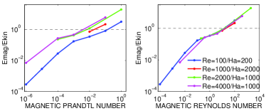
Figure 7: Energy ratio $\varepsilon=E_{\rm mag}/E_{\rm kin}$ for uniform current and rigid rotation, i.e. $\mu=1$. Left: for fixed $\rm{Pm}$ higher magnetic Mach numbers produce higher values of $\varepsilon$. Right: the scaling with $\rm{Rm}$ is rather clear.

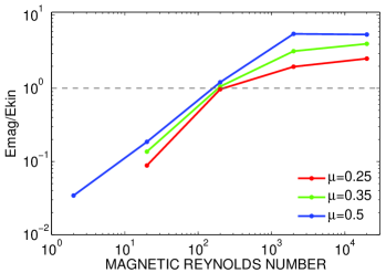
Figure 8: The ratio $\varepsilon$ between magnetic and kinetic energy as a function of $\rm{Rm}$ and $\mu$ for $\mu=0.25/0.35/0.5$. Reynolds number is $\rm{Re}=20000$ for all three configurations, Hartmann number $\rm{Ha}=600$ for $\mu=0.25$, otherwise $\rm{Ha}=1000$.

5 The spectra

5.1 Azimuthal direction

It is typical for the magnetic instability under consideration that i) only nonaxisymmetric modes and ii) only the modes with the lowest $m\neq 0$ become unstable for finite $\rm{Ha}$ and $\rm{Re}$. The rotating pinch gives an example where only a single linearly unstable mode ($m=1$) injects the energy into the system, where the nonlinear interactions transport it to the higher modes. In contrast, for the standard AMRI with $\mu=0.25$ modes with higher $m$ also become unstable if, for a given magnetic field, the system rotates fast enough but not too fast. Figure 1 shows that for given $\rm{Ha}$ and $\rm{Re}$ the number of unstable modes decreases for decreasing magnetic Prandtl number. This is a consequence of the fact that for AMRI all azimuthal modes scale with $\rm{Re}$ and $\rm{Ha}$ for $\rm{Pm}\to 0$. As a consequence, for fixed Reynolds and Hartmann numbers one would expect a spectrum that becomes steeper and steeper already on the large scales (low $m$) with decreasing $\rm{Pm}$. Figure 9 (top) shows the kinetic and magnetic energies for all modes $m$ for this situation of a fixed magnetic field with $\rm{Ha}=600$, and the very high Reynolds number of $\rm{Re}=50000$ and several $\rm{Pm}$. The magnetic and the kinetic spectra have a similar shape, but they are only close together for large $\rm{Pm}$. For small $\rm{Pm}$ the magnetic spectrum lies below the kinetic one, as already demonstrated by Fig. 6. For $\rm{Pm}$ of order unity the spectrum is rather flat (see the blue line corresponding to $\rm{Rm}=50000$) on the low $m$ side, and rather steep for small $\rm{Pm}$, where only one unstable mode exists.

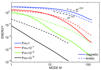
Figure 9: The spectra of the standard AMRI, for various $\rm{Pm}$. Top: The magnetic (solid lines) and the kinetic (dashed lines) energies in the azimuthal Fourier modes $m$ for $\rm{Re}=50000$. Bottom: The magnetic spectra for $\rm{Rm}=10000$. $\rm{Ha}=600$, $\mu=0.25$. The dashed-dotted lines represent the Kolmogorov spectrum and the magnetohydrodynamic IK spectrum.

Magnetic spectra of AMRI for a constant magnetic Reynolds number are shown in the bottom panel of Fig. 9. In this representation the results do not depend on the magnetic Prandtl number. That is, large Reynolds numbers and small $\rm{Pm}$ lead to the same spectra as small Reynolds numbers and large $\rm{Pm}$. The combination of both panels indicates that the spectra become increasingly flat for increasing $\rm{Rm}$. The same is true for $\mu=0.35$, as shown in Fig. 10 for fixed $\rm{Rm}=10000$. The comparison between the spectra of the potential flow $\mu=0.25$ and the quasi-Keplerian $\mu=0.35$ reveals not much difference at the same $\rm{Rm}$. The tails of the spectra become slightly less steep for flatter rotation profiles; the smoothing action of the differential rotation is reduced. The scaling in the intermediate range and large scales is the same; the total amount of magnetic energy in the quasi-Keplerian profile is reduced.

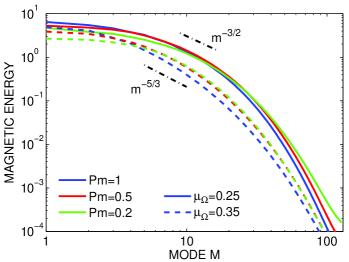
Figure 10: Magnetic energy spectrum for $\rm{Rm}=10000$, comparison of $\mu=0.25$ and $\mu=0.35$.

It is also obvious that the spectra for the kinetic and magnetic fluctuations have similar shapes, and only suggestively show a plateau in the intermediate $m$-range. If a power law is fitted, both would slightly favor the Iroshnikov-Kraichnan (IK) spectrum with $m^{-3/2}$ compared to the Kolmogorov spectrum $m^{-5/3}$, but the differences are small and not significant. Although the IK profile is favored for MHD turbulence (Zhou et al., 2004; Mason et al., 2008), Kolmogorov-like spectra are also known from the measurements of turbulence in the solar wind (Marsch, 2003) as well as the result of 3D MHD simulations (Müller & Biskamp, 2000). Often, however, the direct numerical simulations are done for equipartition ($\varepsilon=1$) and for $\rm{Pm}$ of order unity (see Brandenburg (2014)). One conclusion here could be that this assumption is reasonable if $\rm{Rm}$ is large enough. A clear preference between IK and Kolmogorov scaling cannot be made.

We next return to the question whether the spectra are modified by the number of linearly unstable modes or not. As demonstrated in section 3.2, for the rigidly rotating pinch only $m=1$ becomes unstable. Figure 11 shows the power spectra for this profile for fixed Reynolds and Hartmann number but various magnetic Prandtl numbers. The Mach number varies between $\rm{Mm}=0.2$ for $\rm{Pm}=0.01$ and $\rm{Mm}=2$ for $\rm{Pm}=1$. Only the mode $m=1$ provides the energy to initiate the nonlinear cascade; it is also always $m=1$ that contains the most energy. As expected, the TI spectrum is much steeper than the AMRI spectrum. It is even so steep that neither the IK nor the Kolmogorov spectrum fit the resulting curves. Much closer comes a scaling $m^{-2}$ that is found in forced turbulence (Dallas & Tobias, 2016) or in spectra of not yet truly turbulent flows (Walker et al., 2016). Because the AMRI power spectra for low $\rm{Rm}$ also have a tendency towards $m^{-2}$, this might be a sign of very weak turbulence.

On the other hand, as the energy source in this case is only from the underlying current rather than any differential rotation, one might question whether $\rm{Re}$ and/or $\rm{Rm}$ are the relevant measures at all, or whether $\rm{Ha}$ might not be the more appropriate measure in determining the shape of the spectrum for the rigidly rotating pinch. The largest numerically accessible Hartmann number is $\rm{Ha}\approx 2000$, and still showed no deviation from this $m^{-2}$ scaling.

Figure 11: The spectrum for the rigidly rotating pinch. The magnetic (solid lines) and the kinetic (dashed lines) energies in the azimuthal Fourier modes $m$ for $\rm{Re}=2000$ and $\rm{Ha}=1000$ for various $\rm{Pm}$.

5.2 Axial direction

The spectra in the axial direction have a somewhat different shape compared with the azimuthal direction. The basic wavenumber at the onset of instability is $k\approx 4-5$, corresponding to a round cross section of the patterns. A small increase in the Reynolds number extends this range to $2\lesssim k\lesssim 8$. For turbulence at even higher Reynolds numbers, these large scales remain as a plateau for $k\lesssim 8$, and the part of the spectra for intermediate $k$ shows a similar behavior as the $m$ spectra with no significant plateau (Fig. 12). The closest slope is again the IK profile with $k^{-3/2}$.

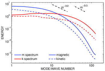
Figure 12: Energy spectra of $m$ and $k$ wavenumbers for $\rm{Rm}=20000,\rm{Ha}=600,\rm{Pm}=1,\mu=0.25$.

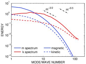
Figure 13: Energy spectra of $m$ and $k$ wavenumbers for $\rm{Rm}=10000,\rm{Ha}=1000,\rm{Pm}=1,\mu=0.35$.

One aspect where the $m$ and $k$ spectra clearly differ is for large values. As previously noted, for large $m$ the spectra drop off quite strongly, due to the smoothing and hence damping effect of the differential rotation. Such a mechanism does not exist in the axial direction, and larger $k$ are correspondingly more strongly excited than large $m$. The greater the shear, the greater the difference between $m$ and $k$ in this regard. For $Rm\approx 20000$ the largest $k$ are stronger by one order of magnitude for the quasi-Keplerian flow, and two orders of magnitude for the steeper potential flow (see Fig. 12 and 13). For the very large $\rm{Rm}$ of real astrophysical objects, this anisotropy between different directions might be even more strongly developed.

6 Summary

Magnetohydrodynamic Taylor-Couette flows have been investigated for many decades (Roberts, 1964). One possibility that is always stable for ideal flows is if the imposed field is purely azimuthal, and has the same radial profile as the imposed velocity profile (Chandrasekhar, 1956). However, as demonstrated by Rüdiger et al. (2015), such Chandrasekhar states can become unstable if at least one of the diffusivities is non-zero. If viscosity and magnetic resistivity are both non-zero, the $m=1$ marginal instability curves in the $\rm{Ha}$-$\rm{Re}$ plane become independent of magnetic Prandtl number in the limit $\rm{Pm}\to 0$. From the definition (13), there will then always exist some (small) value of $\rm{Pm}$ below which all eigenvalues of the linear perturbation equations yield $\rm{Mm}<1$. Given that many cosmical objects such as accretion disks, stars and compact objects often combine small $\rm{Pm}$ and large $\rm{Mm}$, the stability of these Chandrasekhar states might therefore seem to be a purely academic exercise. This is especially the case as for the standard AMRI at least, with ${\it\Omega}\propto 1/R^{2}$ and $B_{\phi}\propto 1/R$, the $m>1$ modes exhibit exactly the same scaling with $\rm{Ha}$ and $\rm{Re}$. Similarly, for the pure TI, with ${\it\Omega}=\rm const$ and $B_{\phi}\propto R$, only the $m=1$ mode is unstable, and it also scales with $\rm{Ha}$ and $\rm{Re}$ for small $\rm{Pm}$.

However, as we demonstrated in this work, for rotation laws between ${\it\Omega}\propto 1/R^{2}$ and ${\it\Omega}=\rm const$ (and corresponding $B_{\phi}\propto R{\it\Omega}$), the $m>1$ modes behave differently, for small $\rm{Pm}$ scaling instead with $\rm{S}$ and $\rm{Rm}$. From the basic relationship $\rm{Mm}=\rm{Rm}/\rm{S}$, together with the upward-sloping shape of the critical stability curve $\rm{Rm}=\rm{Rm}(\rm{S})$, it then follows that $\rm{Mm}>1$ can always be achieved, even in the limit $\rm{Pm}\to 0$. This finding is one of the main conclusions of this work, and suggests that only the $m>1$ modes are relevant for the majority of astrophysical applications.

The magnetic and kinetic energies of MHD instabilities are often considered as approximately the same order when $\rm{Pm}\simeq 1$. For smaller $\rm{Pm}$ the magnetic energy is assumed to be smaller than the kinetic energy (Roberts, 1964). This is indeed true for these Chandrasekhar states. The top panels of Figs. 6 (AMRI) and 7 (TI) show the ratio (17) for the two limiting examples for various $\rm{Pm}$. In both cases the magnetic and kinetic energies are indeed equipartitioned for $\rm{Pm}\simeq 1$, and $\varepsilon\ll 1$ for smaller $\rm{Pm}$. For the curves with fixed $\rm{Ha}$ and $\rm{Re}$ a clear trend exists of the critical $\rm{Pm}$ at the crossing points at the axis $\varepsilon=1$. For a single curve for the pair $[\rm{Ha},\rm{Re}]$ the ratio scales as $\varepsilon\propto\rm{Pm}$, but the curves with other parameter combinations are not identical but rather parallel.

As this conclusion holds for both an example with differential rotation (AMRI) and another one with rigid rotation (TI), the induction by the background flow is obviously not so important. Moreover it is not $\rm{Pm}$ that defines the value of $\varepsilon$. The relevant parameter is the magnetic Reynolds number. This is true not only for the limits $\mu=0.25$ and $\mu=1$, but also for all $\mu$ in between.

For non-magnetic Taylor-Couette flows Dong (2007) simulated turbulent solutions with $r_{\rm in}=0.5$ for flows with resting outer cylinder. The critical Reynolds number for $m=0$ is 68, for $m=1$ it is 75, and for $m=2$ it is 127 (Roberts, 1967). For $\rm{Re}=1000$ the flow is not yet turbulent as no high frequencies appear. For $\rm{Re}=3000$, 5000 and 8000 temporal power spectra of the Kolmogorov-type develop, which only differ slightly for high frequencies. The higher the Reynolds number the higher frequencies appear as more and more nonaxisymmetric modes become unstable. A similar behavior can be observed for the AMRI $m$ spectra of Fig. 9. The bottom panel displays spectra of the magnetic energy for Reynolds numbers from $\rm{Re}=10^{4}$ (blue line) to $\rm{Re}=10^{5}$ (black line). The latter line represents the occurrence of higher frequencies.

The top panel of Fig. 9 demonstrates the influence of the magnetic Prandtl number for given Hartmann and Reynolds numbers, in comparison to the results of Fig. 1. The majority of the modes are unstable for $\rm{Pm}=1$, while for smaller $\rm{Pm}$ (or more general $\rm{Rm}$) the higher modes become more and more stable so that the steepest curve in Fig. 9 (top) results for the smallest $\rm{Pm}$.

The opposite is true for the azimuthal power spectrum of the rigidly-rotating pinch. According to Fig. 11 the curve for $\rm{Pm}=1$ is the steepest. Here only the mode with $m=1$ is unstable, with the strongest rotational suppression for $\rm{Pm}=1$ (see Fig. 3). Even the power spectrum of the rigidly-rotating pinch gives an indication about the double-diffusive character of the nonaxisymmetric magnetic kink-type instability, as analyzed in detail by Rüdiger et al. (2016).

The scaling behavior of the intermediate range of both wavenumbers $m$ and $k$ remains unclear in the sense that no significant plateau develops. The closest scaling exponent will be $m^{-3/2}$ and $k^{-3/2}$ of a Iroshnikov-Kraichnan spectrum. Kolmogorov’s $-5/3$ scaling is not observed.

In comparison to the azimuthal spectra, the axial spectra show a different distribution. First of all there exists a large-scale plateau around the marginal unstable wavenumber $k=4$. The largest wavenumbers are also much more strongly excited. The reason is the smoothing action of differential rotation, which tends to destroy high wavenumbers and leads to a steeper slope in the tails of the $m$ spectra compared with the $k$ spectra. This anisotropy should be even more strongly pronounced for the very large $\rm{Rm}$ of real astrophysical objects.

References

- Acheson (1978) Acheson, D.J. 1978, Phil. Trans. R. Soc. A, 289, 459
- Biskamp (2003) Biskamp, D. 2003, Magnetohydrodynamic Turbulence, Cambridge University Press
- Brandenburg & Subramanian (2005) Brandenburg, A, & Subramanian, K. 2005, Phys. Rep., 417, 1
- Brandenburg (2014) Brandenburg, A. 2014, ApJ, 791, 12
- Chandrasekhar (1956) Chandrasekhar, S. 1956, Proc. Natl. Acad. Sci. USA, 42, 273
- Dallas & Tobias (2016) Dallas, V., & Tobias, S. M. 2016, arXiv:1601.04310
- Dong (2007) Dong, S. 2007, J. Fluid Mech., 587, 373
- Elstner et al. (2014) Elstner, D., Beck, R., & Gressel, O. 2014, A& A, 568, 104
- Fearn (1983) Fearn, D.R. 1983, GAFD, 27, 137
- Gough (2003) Gough, D.O. 2003, in The Solar Tachocline, Cambridge University Press
- Guseva et al. (2015) Guseva, A., Willis, A.P., Hollerbach, R. & Avila, M. 2015, New J. Phys., 17, 093018
- Herron & Soliman (2006) Herron, I., & Soliman, F. 2006, Appl. Math. Lett., 19, 1113
- Hollerbach et al. (2010) Hollerbach, R., Teeluck, V., & Rüdiger, G. 2010, Phys. Rev. Lett., 104, 044502
- Marsch (2003) Marsch, E. 2003, in Physics of the inner Heliosphere, eds. R. Schwenn & E. Marsch, Springer Berlin
- Mason et al. (2008) Mason, J., Cattaneo, F., & Boldyrev, F. 2008, Phys. Rev. E, 77, 6403
- Michael (1954) Michael, D. 1954, Mathematica, 1, 45
- Müller & Biskamp (2000) Müller, W.-C., Biskamp, D. 2000, Phys. Rev. Lett., 84, 475
- Pitts & Tayler (1985) Pitts, E., & Tayler, R.J. 1985, MNRAS, 216, 139
- Roberts (1964) Roberts, P.H. 1964, Proc. Camp. Phil. Soc., 60, 635
- Roberts (1967) Roberts, P.H. 1967, Proc. R. Soc. London A, 300, 94
- Rüdiger et al. (2007) Rüdiger, G., Schultz, M., Shalybkov, D., & Hollerbach, R. 2007, Phys. Rev. E, 76, 056309
- Rüdiger & Schultz (2010) Rüdiger, G., & Schultz, M. 2010, Astron. Nachr., 331, 121
- Rüdiger et al. (2013) Rüdiger, G., Kitchatinov, L.L., & Hollerbach, R. 2013, Magnetic Processes in Astrophysics, Wiley-VCH
- Rüdiger et al. (2014) Rüdiger, G., Gellert, M., Schultz, M., et al. 2014, MNRAS, 438, 271
- Rüdiger et al. (2015) Rüdiger, G., Gellert, M., Spada, F., et al. 2015 A& A, 573, 80
- Rüdiger et al. (2015) Rüdiger, G., Schultz, M., Stefani, F. , & Mond, M. 2015, ApJ, 573, 80
- Rüdiger et al. (2016) Rüdiger, G., Schultz, Gellert, M., & Stefani, F. 2016, Phys. Fluids, 28, 014105
- Seilmayer et al. (2012) Seilmayer, M., Stefani, F., Gundrum, Th., et al. 2012, Phys. Rev. Lett., 108, 244501
- Seilmayer et al. (2014) Seilmayer, M., Galindo, V., Gerbeth, G., et al. 2014, Phys. Rev. Lett., 113, 24505
- Tataronis & Mond (1987) Tataronis, J.A. & Mond, M. 1987, Phys. Fluids, 30, 84
- Tayler (1957) Tayler, R.J. 1957, Proc. Physical Soc., 70, 31
- Tayler (1973) Tayler, R.J. 1973, MNRAS, 161, 365
- Vandakurov (1972) Vandakurov, Y.V. 1972, Sov. Astron, 16, 265
- Walker et al. (2016) Walker, J., Lesur, G., & Boldyrev, S. 2016, MNRAS, 457, L39
- Zhou et al. (2004) Zhou, Ye., Matthaeus, W.H. & Dmitruk, P. 2004, Rev. Mod. Phys. 76, 1015