Lens Depth Function and $k$-Relative Neighborhood Graph: Versatile Tools for Ordinal Data Analysis

Abstract

In recent years it has become popular to study machine learning problems in a setting of ordinal distance information rather than numerical distance measurements. By ordinal distance information we refer to binary answers to distance comparisons such as $d(A,B)<d(C,D)$. For many problems in machine learning and statistics it is unclear how to solve them in such a scenario. Up to now, the main approach is to explicitly construct an ordinal embedding of the data points in the Euclidean space, an approach that has a number of drawbacks. In this paper, we propose algorithms for the problems of medoid estimation, outlier identification, classification, and clustering when given only ordinal data. They are based on estimating the lens depth function and the $k$-relative neighborhood graph on a data set. Our algorithms are simple, are much faster than an ordinal embedding approach and avoid some of its drawbacks, and can easily be parallelized.

Keywords: ordinal data, ordinal distance information, comparison-based algorithms, lens depth function, $k$-relative neighborhood graph, ordinal embedding, non-metric multidimensional scaling

1 Introduction

In a typical machine learning setting we are given a data set ${\cal D}$ of objects together with a dissimilarity function $d$ (or a similarity function $s$) quantifying how “close” objects are to each other. The machine learning rationale is that objects that are close to each other tend to have the same class label, belong to the same clusters, and so on. However, in recent years a whole new branch of the machine learning literature has emerged that relaxes this scenario (e.g., Agarwal et al., 2007, Jamieson and Nowak, 2011, van der Maaten and Weinberger, 2012, Heikinheimo and Ukkonen, 2013, Kleindessner and von Luxburg, 2014, Terada and von Luxburg, 2014, Jain et al., 2016; see Section 5.1 for a discussion of related work). Instead of being able to evaluate the dissimilarity function $d$ itself, we only get to see binary answers to some comparisons of dissimilarity values such as

$$d(A,B)\stackrel{{\scriptstyle?}}{{<}}d(C,D),$$ (1)

where $A,B,C,D\in{\cal D}$. We refer to any collection of answers to such comparisons, some of them possibly being incorrect, as ordinal distance information or ordinal data.

Besides theoretical interest, there are several real-life motivations for studying machine learning tasks in a setting of ordinal distance information:

• Human-based computation / crowdsourcing: In complex tasks, such as estimating the value of a car shown in an image or clustering biographies of celebrities, it can be hard to come up with a meaningful dissimilarity function that can be evaluated automatically, while humans often have a good sense of which objects should be considered (dis-)similar. It is then natural to incorporate the human expertise into the machine learning process. As it is a general phenomenon that humans are significantly better at comparing stimuli than at identifying a single one (Stewart et al., 2005), it is widely believed and accepted that humans are also better and more reliable in assessing dissimilarity on a relative scale (“Movie $A$ is more similar to movie $B$ than movie $C$ is to movie $D$”) than on an absolute one (“The dissimilarity between $A$ and $B$ is 0.3 and the dissimilarity between $C$ and $D$ is 0.8”). For this reason, ordinal questions are often used whenever humans are involved in gathering distance information. In addition to obtaining more robust results, this also has the advantage that one does not need to align people’s different assessment scales.

• There are situations where ordinal distance information is readily available, but the underlying dissimilarity function is completely in the dark. Schultz and Joachims (2003) provide the example of search-engine query logs: if a user clicks on two search results, say $A$ and $B$, but not on a third result $C$, then $A$ and $B$ can be assumed to be semantically more similar than $A$ and $C$, or $B$ and $C$, are.

• There are several applications where actual dissimilarity values between objects can be collected, but it is clear to the practitioner that these values only reflect a rough picture and should be considered informative only on an ordinal scale level. In this case, feeding the numerical scores to a machine learning algorithm can offer the problem that the algorithm interprets them stronger than they are meant to be. For example, discarding the actual values of signal strength measurements but only keeping their order can help to reduce the influence of measurement errors and thus bring some benefit in sensor localization (Liu et al., 2004; Xiao et al., 2006).

A big part of the literature on ordinal data deals with the problem of ordinal embedding. Given a data set ${\cal D}$ together with ordinal relationships, the goal is to map the objects in ${\cal D}$ to points in a Euclidean space $\mathbb{R}^{m}$ such that the ordinal relationships are preserved, with respect to the Euclidean interpoint distances, as well as possible. Clearly, ordinal embedding is a way of transforming ordinal data back to a standard setting: once ${\cal D}$ is represented by points in $\mathbb{R}^{m}$, we can apply any machine learning algorithm for vector-valued data. However, such a two-step approach comes with a number of problems, among them the high running time of ordinal embedding algorithms and the necessity to choose a dimension $m$ for the space of the embedding (to name just two—see Section 5.1.2 for a complete discussion). Our aim is to solve machine learning problems in a setting of ordinal distance information directly, without constructing an ordinal embedding as an intermediate step.

There exist several different approaches in which ordinal relationships can be evaluated (see Section 5.1.1 for more discussion and references). While comparisons of the form $d(A,B)\stackrel{{\scriptstyle\mbox{\tiny?}}}{{<}}d(C,D)$ as in (1) are the most general form, there are other forms that, depending on the application, are of higher relevance. In particular in scenarios of human-based computation and crowdsourcing it is popular to show three objects $A$, $B$, and $C$ at a time and to ask for information on $d(A,B)\stackrel{{\scriptstyle\mbox{\tiny?}}}{{<}}d(A,C)$, that is, compared to (1), object $D$ equals object $A$ (“Which of the bottom two images is more similar to the top one?”). Recently, Heikinheimo and Ukkonen (2013) proposed an algorithm for estimating a medoid of a data set ${\cal D}$ based on statements of the form

$$\text{\emph{Object $A$ is the outlier within the triple of objects $(A,B,C)$}}, \boxplus$$ ()

where $A,B,C$ are pairwise distinct objects in ${\cal D}$ and such a statement formally means that

$$\big{(}d(A,B)>d(B,C)\big{)}\;\;\wedge\;\;\big{(}d(A,C)>d(B,C)\big{)}.$$

Statements of the kind ($\boxplus$ ‣ 1) can easily be collected via crowdsourcing too (“Which among the following three images is the odd one out?”). In this paper, we suggest and study a similar but subtly different kind of question. Given three objects, we ask which of the objects is “the most central” object in the sense that it is the best representative for the three objects. The answers then have the form

Object $$A (A,B,C) \star$$ is the most central object within the triple of objects ()

with the formal interpretation that

$$\big{(}d(A,B)<d(B,C)\big{)}\;\;\wedge\;\;\big{(}d(A,C)<d(B,C)\big{)}.$$

An illustration of the meaning of a statement of the kind ($\star$ ‣ 1) is provided in Figure 1 (left) by an example of a triple of cars consisting of a sports car, a fire truck, and an off-road vehicle: the sports car and the fire truck are rather different, but the off-road vehicle is not so different from either of them and can most likely be taken for a representative of the three cars—the off-road vehicle is the most central object within the triple.

Considering machine learning problems when given only ordinal data, in many cases it is pretty unclear how to solve them other than by constructing an ordinal embedding. For example, how can we construct a classifier based solely on a collection of answers to distance comparisons of the form (1)? The most important insight of this paper is that ordinal distance information in the form ($\star$ ‣ 1) (but not in other forms—in particular, not in the form ($\boxplus$ ‣ 1)) can immediately be related to two very helpful tools: depth functions and relative neighborhood graphs.

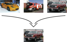
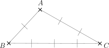
Figure 1: Illustration of the meaning of statement of the kind ($\star$ ‣ 1). Left: Within the three cars shown at the top, the off-road vehicle shown at the bottom a second time is the most central/best representative one. Right: A more formal approach: we have $d(A,B)<d(A,C)<d(B,C)$, and hence $A$ is the most central data point within $(A,B,C)$.

In a nutshell, depth functions (see, e.g., Mosler, 2013) come from multivariate statistics and are a means to generalize the concept of a univariate median to multivariate distributions and to quantify “centrality” of points with respect to such a distribution. The relative neigborhood graph (RNG; Toussaint, 1980) and its generalization, the $k$-RNG, are examples of proximity graphs, which play a prominent role in computer vision. In a proximity graph two vertices are connected by an edge if and only if the two vertices are in some sense close to each other. It is known from the literature that both depth functions and relative neigborhood graphs can be used to solve various machine learning problems. Our contribution is to establish that one particular depth function, the lens depth function (Liu and Modarres, 2011), as well as the $k$-RNG can be computed given the correct statements of the kind ($\star$ ‣ 1) for every triple of objects of ${\cal D}$, but nothing else. More importantly, the lens depth function and the $k$-RNG can be estimated when given not all but only some of possibly incorrect statements of the kind ($\star$ ‣ 1). This leads to algorithms solely based on ordinal data for four common machine learning problems, namely the problems of medoid estimation, outlier identification, classification, and clustering. Our algorithms are simple and can easily and highly efficiently be parallelized. We ran several experiments to compare our algorithms to competitors, in particular to the approach of first solving the ordinal embedding problem and then applying vector-based algorithms. We find that in situations with small sample size and small dimensions, the embedding approach tends to be superior to our algorithms in terms of error rates, while our algorithms are highly superior in terms of computing time (even without parallelization). The strength of our algorithms lies in the regime where the ordinal embedding algorithms break down due to computational complexity, but our algorithms still yield useful results. In any situation, our methods avoid some of the drawbacks inherent in an embedding approach.

The paper is organized as follows: We start with the setup including assumptions on the dissimilarity function $d$ in Section 2. In Section 3 we formally define the lens depth function and the $k$-RNG and establish their relationships to ordinal data of the form ($\star$ ‣ 1). Furthermore, we motivate how we can make use of these relationships in order to solve the machine learning problems of medoid estimation, outlier identification, classification, and clustering when the only available information about a data set ${\cal D}$ is an arbitrary collection of statements of the kind ($\star$ ‣ 1). We formally state our proposed algorithms and discuss their running times, space requirements, and some implementation aspects in Section 4. Related work and further background are presented in Section 5. In Section 6 we present experiments on both artificial and real data. The paper concludes with a discussion and several directions to future work in Section 7.

2 Setup

Let $\mathcal{X}$ be an arbitrary set and $d:\mathcal{X}\times\mathcal{X}\rightarrow\mathbb{R}$ be a dissimilarity function on $\mathcal{X}$: a higher value of $d$ means that two elements of $\mathcal{X}$ are more dissimilar to each other. The terms dissimilarity and distance are used synonymously. We assume $d$ to satisfy the following properties for all $x,y\in\mathcal{X}$:

• $d(x,y)\geq 0$

• $d(x,y)=0$ if and only if $x=y$

• $d(x,y)=d(y,x)$, that is $d$ is symmetric.

With these properties, $(\mathcal{X},d)$ is a semimetric space. Note that we do not require $d$ to satisfy the triangle inequality, and hence $(\mathcal{X},d)$ is not necessarily a metric space. In the following, we consider a finite subset ${\cal D}\subseteq\mathcal{X}$ and refer to ${\cal D}$ as a data set and to the elements of ${\cal D}$ as objects or data points.

We do not have access to $d$ for evaluating dissimilarities between objects directly. Instead, we are only given an arbitrary collection $\mathcal{S}$ of statements

$$\text{\emph{Object $A$ is the most central object within the triple of objects $(A,B,C)$}}, \star$$ ()

where $(A,B,C)$ could be any triple of pairwise distinct objects in ${\cal D}$. At this point we do not make any assumptions on how $\mathcal{S}$ is related to the set of all statements, that is the set of statements of the kind ($\star$ ‣ 1) for all triples of objects (e.g., sampled uniformly at random). However, we need to make some assumptions if we want to provide a theoretical justification for our proposed algorithms (compare with Section 3.1 and Section 3.2.1). Statement ($\star$ ‣ 1) is equivalent to

$$\big{(}d(A,B)<d(B,C)\big{)}\;\;\wedge\;\;\big{(}d(A,C)<d(B,C)\big{)}.$$ (2)

Hence, the most central data point within a triple of data points is the data point opposite to the longest side in the triangle spanned by the three data points. An illustration of this can be seen in Figure 1 (right). Note that if we assume that there are no ties in the total order of all dissimilarities between objects, there is a unique most central object within every triple of objects. Also note that (2) is equivalent to

$$\big{(}d(A,B)+d(A,C)\big{)}<\big{(}d(B,A)+d(B,C)\big{)}\;\wedge\;\big{(}d(A,B)+d(A,C)\big{)}<\big{(}d(C,A)+d(C,B)\big{)},$$

and thus $A$ is the medoid of $\{A,B,C\}$ (see Section 3.1 if you want to recall the definition of a medoid).

Statements might be repeatedly present in $\mathcal{S}$. More importantly, we allow $\mathcal{S}$ to be noisy due to errors in the measurement process and even inconsistent. Noisy means that $\mathcal{S}$ might comprise incorrect statements claiming that, for example, object $A$ is the most central object within $(A,B,C)$ although in fact object $B$ is the most central one. Inconsistent means that we might have contradicting statements: one statement claims that object $A$ is the most central object within $(A,B,C)$, but another one claims that object $B$ is. Noisy and inconsistent ordinal data is likely to be encountered in any real-world problem—think of a crowdsourcing setting, where different users will have different opinions from time to time.

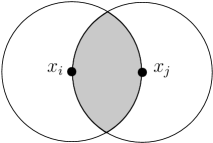
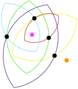
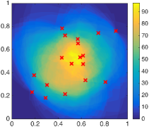
Figure 2: Left: Illustration of $Lens(x_{i},x_{j})$ in case of the Euclidean plane. The lens is shown in grey. Middle: The pink point at the center is contained in almost every lens spanned by any of two data points, while the orange one located at the bottom right edge of the point set is not contained in a single lens. Right: Heat map of the lens depth function for a data set of 18 points (in red) in the unit square of the Euclidean plane.

3 Lens Depth Function and $k$-Relative Neighborhood Graph and Motivation for our Algorithms

The most important geometric object in the following is the lens spanned by two points $x_{i},x_{j}\in\mathcal{X}$. Consider a ball of radius $d(x_{i},x_{j})$ centered at $x_{i}$, and similarly a ball of the same radius centered at $x_{j}$. The lens spanned by $x_{i}$ and $x_{j}$ consists of all those points of $\mathcal{X}$ that are located in the intersection of these two balls. Formally,

$$Lens(x_{i},x_{j}) =\{x\in\mathcal{X}:d(x,x_{i})<d(x_{i},x_{j})\}\cap\{x\in\mathcal{X}:d(x,x_{j})<d(x_{i},x_{j})\}$$

$$=\big{\{}x\in\mathcal{X}:\max\{d(x,x_{i}),d(x,x_{j})\}<d(x_{i},x_{j})\big{\}}.$$

An illustration of $Lens(x_{i},x_{j})$ in case of the Euclidean plane can be seen on the left side of Figure 2. The key insight for us are the following equivalences:

$$\begin{split}x\in Lens(x_{i},x_{j})\Leftrightarrow\\ d(x,x_{i})<d(x_{i},x_{j})~{}\text{and}~{}d(x,x_{j})<d(x_{i},x_{j})\Leftrightarrow\\ \text{$x$ is the most central point within $(x,x_{i},x_{j})$.}\end{split}$$ (3)

In particular, if we had knowledge of all ordinal relationships of type ($\star$ ‣ 1) for a data set ${\cal D}\subseteq\mathcal{X}$, we could check for any data point $x_{k}$ and any two data points $x_{i},x_{j}$ whether $x_{k}$ is contained in $Lens(x_{i},x_{j})$ or not.

3.1 Lens Depth Function

The lens depth function (Liu and Modarres, 2011) is an instance of a statistical depth function. These functions are a widely known tool in multivariate statistics. They have been designed to measure centrality with respect to point clouds or probability distributions. We will provide more information about statistical depth functions in general, including references, in Section 5.2. What makes the lens depth function special for us is that it does not rely on Euclidean structures or numeric distance values. This is in contrast to all other depth functions from the literature. Given a data set ${\cal D}=\{x_{1},\ldots,x_{n}\}\subseteq\mathcal{X}$, the lens depth function $LD({}\cdot{};{\cal D}):\mathcal{X}\rightarrow\mathbb{N}_{0}$ is defined as

$$LD(x;{\cal D})=\big{|}\left\{(x_{i},x_{j}):x_{i},x_{j}\in{\cal D},i<j,x\in Lens(x_{i},x_{j})\right\}\big{|},\quad x\in\mathcal{X}.$$

To understand its meaning, consider a set of data points in the Euclidean plane. A point located at the “heart of the set” will lie in the lenses of many pairs of data points. Thus the lens depth function will attain a high value at this point, indicating its high centrality. In contrast, points at the boundary of the point cloud will lie in only a few lenses and will have a low lens depth value, indicating their low centrality. See the middle sketch of Figure 2 for an illustration. The right side of Figure 2 shows a heat map of the lens depth function for a data set consisting of 18 points in the Euclidean plane as an example.

Exploiting (3) we can see immediately how easily the lens depth function can be evaluated based on statements of the kind ($\star$ ‣ 1). Given all statements of the kind ($\star$ ‣ 1) for a data set $\mathcal{D}=\{x_{1},\ldots,x_{n}\}$, that is one statement for every unordered triple $(x_{i},x_{j},x_{k})$ of pairwise distinct objects in $\mathcal{D}$, we can immediately evaluate $LD(x_{t};{\cal D})$ for any $t\in\{1,\ldots,n\}$. It simply holds that

$$LD(x_{t};{\cal D})=\text{number of statements comprising $x_{t}$ as most central data point.}$$ (4)

We note that $LD(x_{t};{\cal D})$ as given in (4) can be considered, up to a normalizing constant of $1/\binom{n-1}{2}$, as probability of the fixed data point $x_{t}$ being the most central data point in a triple comprising $x_{t}$ and two data points drawn uniformly at random without replacement from ${\cal D}\setminus\{{x_{t}}\}$. This insight gives us a handle for the realistic situation that we are not given all statements of the kind ($\star$ ‣ 1), but only an arbitrary collection $\mathcal{S}$ of statements, some of them possibly being incorrect. Namely, we can still estimate $LD(x_{t};{\cal D})$ by estimating the probability of the described event by its relative frequency:

$$LD(x_{t};{\cal D})\stackrel{{\scriptstyle\cdot}}{{\approx}}\frac{\text{number of statements in $\mathcal{S}$ that comprise $x_{t}$ as most central data point}}{\text{number of statements in $\mathcal{S}$ that comprise $x_{t}$}}.$$ (5)

This estimate will be reasonable whenever statements in $\mathcal{S}$ comprising $x_{t}$ appear to be sampled approximately uniformly at random from the set of all statements that comprise $x_{t}$, the number of statements in $\mathcal{S}$ comprising $x_{t}$ is large enough, and the proportion of incorrect statements is sufficiently small. Note that if we assume $\mathcal{S}$ to be sampled uniformly at random from the set of all statements, this will imply that for every $x_{t}\in{\cal D}$ statements in $\mathcal{S}$ comprising $x_{t}$ are a uniform sample from the set of all statements that comprise $x_{t}$.

We now explain how we can use our insights to devise algorithms for the machine learning problems of medoid estimation, outlier identification, and classification when only given a collection of statements of the kind ($\star$ ‣ 1) for a data set (the algorithms are formally stated in Section 4). The basic principle is that we replace the true lens depth function with its estimate according to (5) in the following existing approaches to these problems (see Section 5.2 for further information and references):

• Medoid estimation (cf. Algorithm 1 in Section 4): A medoid $O_{\text{MED}}$ of a data set ${\cal D}$ is a most central object in the sense that it has minimal total distance to all other objects, that is it minimizes

  $$D(O)=\sum_{O_{i}\in\mathcal{D}}d(O,O_{i}),\quad O\in\mathcal{D}.$$ (6)

  Since the lens depth function provides a measure of centrality too, even though in a different sense, a maximizer of the lens depth function (restricted to ${\cal D}$) is a natural candidate for an estimate of a medoid.

• Outlier identification (cf. Algorithm 2 in Section 4): An outlier in a data set ${\cal D}$ is “an observation . . . which appears to be inconsistent with the remainder of that set of data” (Barnett and Lewis, 1978, Chapter 1). Points with a low lens depth value are non-central points according to the lens depth function and thus are natural candidates for outliers. We will see in the experiments in Section 6.1.2 that this approach works well for data sets with a uni-modal structure, but can fail in multi-modal cases.

  

  

  

  

  

  

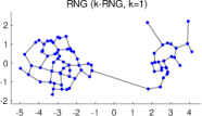
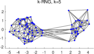
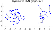
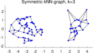
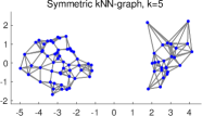
  Figure 3: $k$-relative neighborhood graphs (1st row) and symmetric $k$-nearest neighbor graphs (2nd row) on 80 points from a mixture of two Gaussians. Note that as opposed to the $k$-NN graphs, the $k$-relative neighborhood graphs tend to have more connections between points from the different mixture components. In fact, a $k$-RNG is always connected (see Section 5.3). This might be desirable in some situations, but undesirable in others.

• Classification (cf. Algorithm 3 in Section 4): The simplest approach to classification based on the lens depth function is to assign a test point to that class in which it is a more central point: For each of the classes we could compute a separate lens depth function and evaluate a test point’s corresponding depth value. The test point is then classified as belonging to the class that gives rise to the highest lens depth value. However, it has been found that such a max-depth approach has some severe limitations (compare with Section 5.2).

  To overcome these limitations, we use a feature-based approach. When dealing with a $K$-class classification problem, we consider the data-dependent feature map

  $$x\mapsto(LD(x;Class_{1}),LD(x;Class_{2}),\ldots,LD(x;Class_{K}))\in\mathbb{R}^{K},\quad x\in\mathcal{X},$$ (7)

  and then apply an out-of-the-box classification algorithm to the $K$-dimensional representation of the data set.

3.2 $k$-Relative Neighborhood Graph

We now use the lenses spanned by two data points in order to define the $k$-relative neighborhood graph ($k$-RNG). In our language, for a data set $\mathcal{D}=\{x_{1},\ldots,x_{n}\}\subseteq\mathcal{X}$ and a parameter $k\in\mathbb{N}$ the $k$-RNG on ${\cal D}$ is the graph with vertex set ${\cal D}$ in which two distinct vertices $x_{i}$ and $x_{j}$ are connected by an undirected edge if and only if the lens spanned by these points contains fewer than $k$ data points from ${\cal D}$:

$$x_{i}\sim x_{j}~{}\Leftrightarrow~{}\left|Lens(x_{i},x_{j})\cap{\cal D}\right|<k.$$ (8)

The rationale behind this definition is that two data points may be considered close to each other whenever the lens spanned by them contains only a few data points. The $k$-relative neighborhood graph is best known when $k=1$. In this form it is simply called relative neighborhood graph (RNG) and has already been introduced in Toussaint (1980). The general $k$-RNG has been defined by Chang et al. (1992). Examples for a data set in the Euclidean plane can be seen in Figure 3. For comparison, we also also show symmetric $k$-nearest neighbor graphs on the data set. The symmetric $k$-nearest neighbor graph or $k$-NN graph for short, also with parameter $k\in\mathbb{N}$, is more popular in machine learning. In that graph two vertices are connected by an undirected edge whenever one of them is among the $k$ closest data points to the other one (with respect to the distance function $d$).

Given all statements of the kind ($\star$ ‣ 1) for a data set ${\cal D}$, it is straightforward to build the true $k$-RNG on ${\cal D}$ similarly to the exact evaluation of the lens depth function (4). Below, we will discuss how to build an estimate of the $k$-RNG on ${\cal D}$ when given only an arbitrary collection of statements, some of them possibly being incorrect, and a problem involved in Section 3.2.1. Before, let us explain how $k$-relative neighborhood graphs can be used for classification and clustering.

• Classification (cf. Algorithm 4 in Section 4): Given a set of labeled points and an additional test point that we would like to classify, we can construct the $k$-RNG on the union of the set of labeled points and the singleton of the test point and take a majority vote of the test point’s neighbors in the graph. There is no need to construct the whole graph. We just have to find the test point’s neighbors in the graph. Note that the basic principle is the same as for the well-known $k$-NN classifier (e.g., Shalev-Shwartz and Ben-David, 2014, Chapter 19), replacing the directed $k$-NN graph by the $k$-RNG.

• Clustering (cf. Algorithm 5 in Section 4): As we can do with the symmetric $k$-NN graph, it is straightforward to apply spectral clustering to the $k$-RNG on a data set ${\cal D}$ (see von Luxburg, 2007, for a comprehensive introduction to spectral clustering—that work suggests the symmetric $k$-NN graph as one of a few graphs that can be used). We propose two versions: one is to simply work with an estimate of the ordinary unweighted $k$-RNG, the other one is to use an estimate of a $k$-RNG in which an edge between connected vertices $x_{i}$ and $x_{j}$ is weighted by

  $$\exp\left(-\frac{1}{\sigma^{2}}\cdot\frac{|Lens(x_{i},x_{j})\cap{\cal D}|^{2}}{(|{\cal D}|-2)^{2}}\right)$$ (9)

  for a scaling parameter $\sigma>0$.

3.2.1 The Problem of Estimating the $k$-RNG from Noisy Ordinal Data

The key insight for estimating the $k$-RNG on a data set ${\cal D}$ from ordinal distance information of type ($\star$ ‣ 1) is similar to the one for estimating the lens depth function: the characterization (8) is equivalent to two distinct, fixed data points $x_{i}$ and $x_{j}$ being connected in the $k$-RNG if and only if the probability of a data point drawn uniformly at random from ${\cal D}\setminus\{x_{i},x_{j}\}$ lying in $Lens(x_{i},x_{j})$ is smaller than $k/(|{\cal D}|-2)$. Given a collection $\mathcal{S}$ of statements of the kind ($\star$ ‣ 1), this probability can be estimated by

$$V(x_{i},x_{j})=\frac{N(x_{i},x_{j})}{D(x_{i},x_{j})},$$ (10)

where

$$\begin{split}N(x_{i},x_{j})&=\text{number of statements in $\mathcal{S}$ comprising both $x_{i}$ and $x_{j}$ and}\\ &\text{~{}~{}~{}~{}another data point as most central data point},\\ D(x_{i},x_{j})&=\text{number of statements in $\mathcal{S}$ comprising both $x_{i}$ and $x_{j}$}.\end{split}$$ (11)

Thus our strategy to estimate the $k$-RNG on ${\cal D}$ is the following: we connect two data points $x_{i}$ and $x_{j}$ with $i\neq j$ by an undirected edge if and only if

$$V(x_{i},x_{j})<\frac{k}{|{\cal D}|-2}.$$ (12)

If all statements in $\mathcal{S}$ are correct and, for every $x_{i}$ and $x_{j}$ with $i\neq j$, there are sufficiently many statements in $\mathcal{S}$ that comprise both $x_{i}$ and $x_{j}$ and these statements appear to be sampled approximately uniformly at random from the set of all statements that comprise $x_{i}$ and $x_{j}$, we can expect our estimate of the $k$-RNG to be reasonable.

However, incorrect statements in $\mathcal{S}$ create a problem for our strategy. Usually, we are interested in a $k$-RNG for a small value of the parameter $k$, aiming at connecting only data points that are close to each other. Consequently, according to (12), in order that the data points $x_{i}$ and $x_{j}$ are connected in our estimate of the $k$-RNG, the estimated probability $V(x_{i},x_{j})$ has to be small. However, in case of erroneous ordinal data comprising sufficiently many incorrect statements, there will always be statements wrongly indicating that there are some data points in $Lens(x_{i},x_{j})$ that in fact are not, and thus $V(x_{i},x_{j})$ will always be somewhat large. Hence, many of the edges of the true $k$-RNG on ${\cal D}$ will not be present in our estimate.

To make this formal, consider the following simple noise model: Statements of the kind ($\star$ ‣ 1) are incorrect, independently of each other, with some fixed probability $errorprob$. In an incorrect statement the two data points that are not most central appear to be most central with probability $1/2$ each. In our experiments in Section 6.1, this noise model is referred to as Noise model I. Assume $\mathcal{S}$ to be sampled uniformly at random from all statements. Denote by $p=p(x_{i},x_{j})$ the probability that a data point drawn uniformly at random from ${\cal D}\setminus\{x_{i},x_{j}\}$ lies in $Lens(x_{i},x_{j})$, that is $p=|Lens(x_{i},x_{j})\cap{\cal D}|/(|{\cal D}|-2)$. Denote by $\tilde{p}=\tilde{p}(x_{i},x_{j})$ the probability that the following experiment yields a positive result: A data point is drawn uniformly at random from ${\cal D}\setminus\{x_{i},x_{j}\}$. Independently, a Bernoulli trial with a probability of success equaling $errorprob$ is performed. If the Bernoulli trial fails, the experiment yields a positive result if and only if the drawn data point falls into $Lens(x_{i},x_{j})$. If the Bernoulli trial succeeds, the experiment yields a positive result if and only if the data point does not fall into $Lens(x_{i},x_{j})$ and another Bernoulli trial, with a probability of success of one half and performed independently, succeeds. It is clear that under the considered model, $V(x_{i},x_{j})$ as given in (10) and (11) is an estimate of $\tilde{p}$ rather than of $p$. Assuming that $errorprob$ is less than $2/3$, we can relate $\tilde{p}$ and $p$ via

$$\tilde{p}=p\cdot(1-errorprob)+(1-p)\cdot errorprob\cdot\frac{1}{2},$$ (13)

or equivalently

$$p=\frac{\tilde{p}-\frac{1}{2}\cdot errorprob}{1-\frac{3}{2}\cdot errorprob}.$$ (14)

The probability $\tilde{p}$ is obtained from $p$ by applying an affine transformation and vice versa.

It follows from (13) that our strategy yields an estimate of the $k^{\prime}$-RNG with

$$k^{\prime}=\frac{k-\frac{1}{2}\cdot errorprob\cdot(|\mathcal{D}|-2)}{1-\frac{3}{2}\cdot errorprob}$$ (15)

rather than of the intended $k$-RNG. In particular, we have $k^{\prime}<k$ for $k<\frac{1}{3}(|{\cal D}|-2)$ and $k^{\prime}\leq 0$ for $k\leq\frac{1}{2}\cdot errorprob\cdot(|\mathcal{D}|-2)$. This means that whenever $k<\frac{1}{3}(|{\cal D}|-2)$, our strategy produces an estimate containing fewer edges than we would like to have, and whenever $k\leq\frac{1}{2}\cdot errorprob\cdot(|\mathcal{D}|-2)$, it even produces an estimate of an empty graph, that is a graph without any edges at all.

These findings might seem worse than they actually are: using our estimated graph for classification or clustering, we do not care whether we work with the estimate of a $k^{\prime}$-RNG instead of a $k$-RNG, but only whether our classification or clustering result is useful. However, we have to bear them in mind when choosing the parameter $k$ in our algorithms: Using cross-validation for choosing $k$ for Algorithm 4 (classification by means of a majority vote of neighbors in the graph), we may only use Leave-one-out cross-validation variants since we have to ensure roughly the same size of the training set during cross-validation and the training set in the ultimate classification task. Otherwise, a value of $k$ that is optimal during cross-validation will not be optimal in the ultimate classification problem since $k^{\prime}$ depends on $|{\cal D}|$ as stated in (15). Applying Algorithm 5 (spectral clustering on the estimated $k$-RNG), we have to choose $k$ so large that the constructed graph is connected. This is not only required by some versions of spectral clustering, but also indicates that the graph is indeed an estimate of a true $k^{\prime}$-RNG with $k^{\prime}\geq 1$ rather than of an empty graph. If we know the value of $errorprob$, or have at least an estimate of it, we can correct for the bias of our strategy. In order to estimate the $k$-RNG on a data set ${\cal D}$ for the intended value of $k$, according to (14), two data points $x_{i}$ and $x_{j}$ with $i\neq j$ should be connected if and only if

$$\frac{V(x_{i},x_{j})-\frac{1}{2}\cdot errorprob}{1-\frac{3}{2}\cdot errorprob}<\frac{k}{|{\cal D}|-2},$$ (16)

which equals (12) if $errorprob=0$. Note that although the left-hand side of equation (16) is an unbiased estimator of $p(x_{i},x_{j})$ for every $x_{i}$ and $x_{j}$ with $i\neq j$ (assuming $\mathcal{S}$ to be sampled uniformly at random from all statements), due to the thresholding step in (16) our estimation strategy is still not an unbiased estimator of the intended $k$-RNG.

4 Algorithms for Medoid Estimation, Outlier Identification, Classification, and Clustering

In this section we formally state our algorithms for the problems of medoid estimation, outlier identification, classification, and clustering when the only available information about a data set ${\cal D}$ is a collection $\mathcal{S}$ of statements of the kind ($\star$ ‣ 1). Furthermore, we discuss running times, space requirements, and some implementation aspects.

4.1 Medoid Estimation

The following Algorithm 1 returns as output an estimate of a medoid of ${\cal D}$ as motivated in Section 3.1. The estimate is given by an object that maximizes the estimated lens depth function on ${\cal D}$. By setting the estimated lens depth value $LD(O)$ to zero for objects $O$ that do not appear in any statement in $\mathcal{S}$, which means that we do not have any information about $O$, we ensure that such an object is never returned as output (unless there is no available information about ${\cal D}$ at all, i.e. $\mathcal{S}=\emptyset$).

Algorithm 1 Estimating a medoid

1:a collection $\mathcal{S}$ of statements of the kind ($\star$ ‣ 1) for some data set ${\cal D}$

2:an estimate of a medoid of ${\cal D}$

3:for every object $O$ in ${\cal D}$ compute

$$LD(O):=\frac{\text{number of statements comprising $O$ as most central object}}{\text{number of statements comprising $O$}}$$

4:$\rhd$ if the denominator equals zero, set $LD(O)=0$

5:return an object $O$ for which $LD(O)$ is maximal

If we assume that every object in ${\cal D}$ can be identified by a unique index from $\{1,\ldots,|{\cal D}|\}$ and, given a statement in $\mathcal{S}$, the indices of the three objects involved can be accessed in constant time, then Algorithm 1 can be implemented with $\mathcal{O}(|{\cal D}|+|\mathcal{S}|)$ time and $\mathcal{O}(|{\cal D}|)$ space in addition to storing $\mathcal{S}$. This can be done by going through $\mathcal{S}$ only once and updating counters for the three objects found in a statement. If the objects in ${\cal D}$ are not indexed by $1,\ldots,|{\cal D}|$, we can use minimal perfect hashing in order to first create such an indexing. This requires about $\mathcal{O}(|{\cal D}|)$ time and space (Hagerup and Tholey, 2001; Botelho et al., 2007), so the overall requirements remain unaffected by this additional step. An important feature of Algorithm 1 is that it can easily be parallelized by partitioning $\mathcal{S}$ into several subsets that may be processed independently. Since one usually may expect that $|\mathcal{S}|\gg|{\cal D}|$, such a parallelization has almost ideal speedup, that is doubling the number of processing elements leads to almost only half of the running time.

4.2 Outlier Identification

By means of the following Algorithm 2 we can identify outliers in ${\cal D}$ given as input only a collection $\mathcal{S}$ of statements of the kind ($\star$ ‣ 1). Outlier candidates are data points with low estimated lens depth values $LD(O)$. By setting $LD(O)$ to zero for objects $O$ that do not appear in any statement we guarantee that such objects are identified as outliers.

Algorithm 2 Identifying outlier candididates

1:a collection $\mathcal{S}$ of statements of the kind ($\star$ ‣ 1) for some data set ${\cal D}$

2:a subset of ${\cal D}$ containing objects that are outlier candidates

3:for every object $O$ in ${\cal D}$ compute

$$LD(O):=\frac{\text{number of statements comprising $O$ as most central object}}{\text{number of statements comprising $O$}}$$

4:$\rhd$ if the denominator equals zero, set $LD(O)=0$

5:identify objects with exceptionally small values of $LD(O)$

6:return the set of identified objects

The only difference between Algorithm 2 and Algorithm 1 is that instead of returning the object with the highest value of $LD(O)$ as estimate of a medoid we return objects with exceptionally small values as outlier candidates. The running time of Algorithm 2 depends on the identification strategy in Step 2, but if one simply identifies $c$ objects with smallest values ($1\leq c\leq|{\cal D}|$), then Algorithm 2 can be implemented with $\mathcal{O}(|{\cal D}|+|\mathcal{S}|)$ time and $\mathcal{O}(|{\cal D}|)$ space in addition to storing $\mathcal{S}$ analogously to Algorithm 1. Here we make use of the fact that the selection of the $c$-th smallest value in an array of length $|{\cal D}|$ can be done in $\mathcal{O}(|{\cal D}|)$ time and space (Blum et al., 1973). Just as for Algorithm 1, the first step of Algorithm 2 can easily be parallelized.

4.3 Classification

We propose two different algorithms for dealing with $K$-class classification in a data set ${\cal D}$ consisting of a subset $\mathcal{L}$ of labeled objects and a subset $\mathcal{U}$ of unlabeled objects when given no more information than the class labels for the objects in $\mathcal{L}$ and a collection $\mathcal{S}$ of statements of the kind ($\star$ ‣ 1) for ${\cal D}$. Our goal is to predict a class label for every object in $\mathcal{U}$.

Our first proposed algorithm, Algorithm 3, is based on the lens depth function and has been motivated in Section 3.1. It consists of computing a feature embedding of ${\cal D}$ into $[0,1]^{K}\subseteq\mathbb{R}^{K}$, in which each feature corresponds to the estimated lens depth value with respect to one class, and subsequently applying a classification algorithm that is suitable for $K$-class classification on $\mathbb{R}^{K}$ to this embedding.

Algorithm 3 $K$-class classification I

1:a collection $\mathcal{S}$ of statements of the kind ($\star$ ‣ 1) for some data set ${\cal D}$ comprising a set $\mathcal{L}$ of labeled objects and a set $\mathcal{U}$ of unlabeled objects; a class label for every labeled object in $\mathcal{L}$ according to its membership in one of $K$ classes (referred to as $Class_{1},\ldots,Class_{K}$) $\rhd$ note that we have ${\cal D}=\mathcal{L}~{}\dot{\cup}~{}\mathcal{U}$ and $\mathcal{L}=Class_{1}~{}\dot{\cup}~{}Class_{2}~{}\dot{\cup}~{}\ldots~{}\dot{\cup}~{}Class_{K}$

2:an inferred class label for every unlabeled object in $\mathcal{U}$

3:for every object $O$ in ${\cal D}$ and $i\in\{1,\ldots,K\}$ compute

$$N_{C_{i}}(O):=\text{number of statements comprising $O$ and two labeled objects from $Class_{i}$}$$

               with $$O$$ as most central object

$$D_{C_{i}}(O):=\text{number of statements comprising $O$ and two labeled objects from $Class_{i}$}$$

$$LD_{C_{i}}(O):=\frac{N_{C_{i}}(O)}{D_{C_{i}}(O)}$$

4:$\rhd$ if $D_{C_{i}}(O)$ equals zero, set $LD_{C_{i}}(O)=0$

5:train an arbitrary classifier (suitable for $K$-class classification on $\mathbb{R}^{K}$) with training data

$$\{(LD_{C_{1}}(O_{l}),LD_{C_{2}}(O_{l}),\ldots,LD_{C_{K}}(O_{l})):O_{l}\in\mathcal{L}\}\subseteq\mathbb{R}^{K}$$

where the label of $(LD_{C_{1}}(O_{l}),LD_{C_{2}}(O_{l}),\ldots,LD_{C_{K}}(O_{l}))$ equals the label of $O_{l}$

6:return as inferred class label of every unlabeled object $O_{u}\in\mathcal{U}$ the label predicted by the classifier applied to $(LD_{C_{1}}(O_{u}),LD_{C_{2}}(O_{u}),\ldots,LD_{C_{K}}(O_{u}))\in\mathbb{R}^{K}$

Assuming that the number of classes $K$ is bounded by a constant, the first step of Algorithm 3 requires $\mathcal{O}(|{\cal D}|+|\mathcal{S}|)$ operations and $\mathcal{O}(|{\cal D}|)$ space in addition to storing $\mathcal{S}$. This is the same as for Algorithm 1 and Algorithm 2. As before, this step can easily and highly efficiently be parallelized (assuming that $|\mathcal{S}|\gg|{\cal D}|$). The time and space complexities of the remaining steps depend on the generic classifier that is used.

Our second proposed algorithm, Algorithm 4, is based on the $k$-RNG and has been motivated in Section 3.2. It is an instance-based learning method like the well-known $k$-NN classifier: There is no explicit training phase involved. An unlabeled object is readily classified by assigning the label that is most frequently encountered among the neighbors of the unlabeled object in the estimated $k$-RNG.

Algorithm 4 $K$-class classification II

1:a collection $\mathcal{S}$ of statements of the kind ($\star$ ‣ 1) for some data set ${\cal D}$ comprising a set $\mathcal{L}$ of labeled objects and a set $\mathcal{U}$ of unlabeled objects; a class label for every labeled object in $\mathcal{L}$ according to its membership in one of $K$ classes (referred to as $Class_{1},\ldots,Class_{K}$); an integer parameter $k$ $\rhd$ note that we have ${\cal D}=\mathcal{L}~{}\dot{\cup}~{}\mathcal{U}$ and $\mathcal{L}=Class_{1}~{}\dot{\cup}~{}Class_{2}~{}\dot{\cup}~{}\ldots~{}\dot{\cup}~{}Class_{K}$

2:an inferred class label for every unlabeled object in $\mathcal{U}$

3:for every unlabeled object $O_{u}\in\mathcal{U}$ and every labeled object $O_{l}\in\mathcal{L}$ compute

$$N(O_{u},O_{l}) :=\text{number of statements comprising both $O_{u}$ and $O_{l}$ and another}$$

     labeled object as most central object

$$D(O_{u},O_{l}) :=\text{number of statements comprising both $O_{u}$ and $O_{l}$ and another}$$

     labeled object

$$V(O_{u},O_{l}) :=\frac{N(O_{u},O_{l})}{D(O_{u},O_{l})}$$

4:  $\rhd$ if $D(O_{u},O_{l})$ equals zero, set $V(O_{u},O_{l})=\infty$

5:return as inferred class label of every unlabeled object $O_{u}\in\mathcal{U}$ the majority vote (ties broken randomly) of the labels of those objects $O_{l}\in\mathcal{L}$ that satisfy

$$V(O_{u},O_{l})<\frac{k}{|\mathcal{L}|-1}$$

Assuming that the number of classes $K$ is bounded by a constant, Algorithm 4 can be implemented with $\mathcal{O}(|{\cal D}|+|\mathcal{U}|\cdot|\mathcal{L}|+|\mathcal{S}|)=\mathcal{O}(|\mathcal{U}|\cdot|\mathcal{L}|+|\mathcal{S}|)$ time and $\mathcal{O}(|{\cal D}|+|\mathcal{U}|\cdot|\mathcal{L}|)=\mathcal{O}(|\mathcal{U}|\cdot|\mathcal{L}|)$ space in addition to storing $\mathcal{S}$. Here we have to assign to each labeled object a unique identifier in $\{1,\ldots,|\mathcal{L}|\}$ and to each unlabeled object a unique identifier in $\{1,\ldots,|\mathcal{U}|\}$ that can be looked up in constant time. This allows us to increment a value of $N(O_{u},O_{l})$ or $D(O_{u},O_{l})$ for $(O_{u},O_{l})\in\mathcal{U}\times\mathcal{L}$ stored in an array of size $|\mathcal{U}|\times|\mathcal{L}|$ within constant time. Once the objects are indexed by $1,\ldots,|{\cal D}|$ (compare with Section 4.1), we can easily assign such identifiers in $\mathcal{O}(|{\cal D}|)$ time and space. Again, it is straightforward to parallelize Algorithm 4 by partitioning $\mathcal{S}$.

4.4 Clustering

Our proposed Algorithm 5 for clustering a data set ${\cal D}$ when only given a collection $\mathcal{S}$ of statements of the kind ($\star$ ‣ 1) as input consists of estimating the $k$-RNG on ${\cal D}$ and applying spectral clustering to the estimate. Note that some versions of spectral clustering require the underlying similarity graph not to contain isolated vertices. A true $k$-RNG never contains isolated vertices since a $k$-RNG is always connected (compare with Section 5.3), but if $k$ is chosen too small, an estimated $k$-RNG might contain isolated vertices (compare with Section 3.2.1).

Algorithm 5 Clustering

1:a collection $\mathcal{S}$ of statements of the kind ($\star$ ‣ 1) for some data set ${\cal D}=\{O_{1},\ldots,O_{n}\}$; an integer parameter $k$; number $l$ of clusters to construct; a parameter $\sigma>0$ in case of weighted version

2:a hard clustering $C_{1},\ldots,C_{l}\subseteq{\cal D}$ with $C_{1}~{}\dot{\cup}~{}C_{2}~{}\dot{\cup}~{}\ldots~{}\dot{\cup}~{}C_{l}={\cal D}$

3:for every pair $(O_{i},O_{j})$ of objects in ${\cal D}$ compute

$$N(O_{i},O_{j}) :=\text{number of statements comprising both $O_{i}$ and $O_{j}$}$$

     and another object as most central object

$$D(O_{i},O_{j}) :=\text{number of statements comprising both $O_{i}$ and $O_{j}$}$$

$$V(O_{i},O_{j}) :=\frac{N(O_{i},O_{j})}{D(O_{i},O_{j})}$$

4:$\rhd$ if $D(O_{i},O_{j})=0$, set $V(O_{i},O_{j})=\infty$  (in particular, $V(O_{i},O_{i})=\infty$ for $i=1,\ldots,n$)

5:let $W=(w_{ij})_{i,j=1,\ldots,n}$ be a $(n,n)$-matrix and either set

$$W_{ij}=\begin{cases}1&\text{if }V(O_{i},O_{j})<{k}/{(|{\cal D}|-2)}\\ 0&\text{else}\end{cases}\qquad~{}~{}~{}~{}~{}~{}~{}\text{$\rhd$ unweighted version}$$

or

$$W_{ij}=\begin{cases}e^{-\frac{V(O_{i},O_{j})^{2}}{\sigma^{2}}}&\text{if }V(O_{i},O_{j})<{k}/{(|{\cal D}|-2)}\\ 0&\text{else}\end{cases}\qquad~{}\text{$\rhd$ weighted version}$$

6:apply spectral clustering to $W$ with $l$ as input parameter for the number of clusters

7:return clusters $C_{1},\ldots,C_{l}$ according to the clusters produced in Step 3

The first step of Algorithm 5 can be implemented with $\mathcal{O}(|{\cal D}|^{2}+|\mathcal{S}|)$ time and $\mathcal{O}(|{\cal D}|^{2})$ space in addition to storing $\mathcal{S}$. It can be parallelized in the same way as the corresponding parts of the previous algorithms. However, here we achieve almost ideal speedup only in case $|\mathcal{S}|\gg|{\cal D}|^{2}$. The second step can be implemented with $\mathcal{O}(|{\cal D}|^{2})$ time and $\mathcal{O}(|{\cal D}|^{2})$ space. The complexity of Step 3 is the one of spectral clustering after the construction of a similarity graph. Its costs are dominated by the complexity of eigenvector computations and are commonly stated to be in general in $\mathcal{O}(n^{3})=\mathcal{O}(|{\cal D}|^{3})$ regarding time and $\mathcal{O}(n^{2})=\mathcal{O}(|{\cal D}|^{2})$ regarding space for an arbitrary number of clusters $l$, unless approximations are applied (Yan et al., 2009; Li et al., 2011). In many cases the estimate of the $k$-RNG constructed by Algorithm 5 might be sparse (compare with Section 5.3), and then the eigenvector computations can be done much more efficiently (Bai et al., 2000). However, in the worst case the overall running time of Algorithm 5 can be up to $\mathcal{O}(|{\cal D}|^{3}+|\mathcal{S}|)$. The overall space requirements are $\mathcal{O}(|{\cal D}|^{2})$ in addition to storing $\mathcal{S}$.

5 Related Work and Further Background

In this section we present related work and further background on ordinal data analysis, statistical depth functions, and the $k$-relative neighborhood graph. In a first reading, the reader may skip this part and go to the experimental Section 6 immediately.

5.1 Machine Learning in a Setting of Ordinal Distance Information

We have mentioned in Section 1 that ordinal data can be distinguished with respect to the kind of ordinal relationships that it consists of and that ordinal embedding is a general approach to machine learning in a setting of ordinal distance information. Here we discuss these two topics in more detail.

5.1.1 Different Types of Ordinal Data

The most general form of ordinal distance information consists of binary answers to some dissimilarity comparisons

$$d(A,B)\stackrel{{\scriptstyle?}}{{<}}d(C,D),$$ (17)

where $A,B,C,D$ could be any objects of some data set. In the machine learning literature, this very general type of ordinal data has been studied in Agarwal et al. (2007), Kleindessner and von Luxburg (2014), Terada and von Luxburg (2014), and Arias-Castro (2015).

The type most often studied in the literature is the one of similarity triplets (Jamieson and Nowak, 2011; Tamuz et al., 2011; van der Maaten and Weinberger, 2012; Wilber et al., 2014; Amid and Ukkonen, 2015; Heim et al., 2015; Amid et al., 2016; Jain et al., 2016; Haghiri et al., 2017). Similarity triplets are answers to dissimilarity comparisons of the restricted form

$$d(A,B)\stackrel{{\scriptstyle?}}{{<}}d(A,C).$$ (18)

Compared to (17), $A$ equals $D$ and serves as an anchor point.

Another well-known type of ordinal data is the directed, but unweighted $k$-nearest neighbor graph on a data set (Shaw and Jebara, 2009; von Luxburg and Alamgir, 2013; Terada and von Luxburg, 2014; Hashimoto et al., 2015; Kleindessner and von Luxburg, 2015). This graph provides the ordinal dissimilarity relationships

$$d(V,N)<d(V,O)$$

for objects $V$, $N$, and $O$ such that $N$ is adjacent to $V$ in the graph, but $O$ is not.

Ordinal distance information in the form ($\star$ ‣ 1), which we consider in this work, is similar to statements of the form (compare with Section 1)

$$\text{\emph{Object $A$ is the outlier within the triple of objects $(A,B,C)$}}. \boxplus$$ ()

This type of ordinal data has been studied by Heikinheimo and Ukkonen (2013) and also by Ukkonen et al. (2015). Heikinheimo and Ukkonen (2013) proposed an algorithm for estimating a medoid of a data set based on statements of the kind ($\boxplus$ ‣ 1). Their approach is closely related to ours (compare with Algorithm 1): For every fixed data point, they estimate the probability that the data point is the outlier within a triple of three data points containing the fixed data point and two data points chosen uniformly at random from the remaining ones. Then they take the data point with minimal estimated probability as an estimate of a medoid. However, the conceptual problem with their approach is that the function that it is based on,

$$F(x;P)=1-Probability(\text{$x$ is the outlier within the triple of points $(x,X,Y)$}),$$ (19)

is not a valid statistical depth function. It does not satisfy one of the most crucial properties of statistical depth functions, namely maximality at the center for symmetric distributions (see Section 5.2). As a consequence, their approach always fails to return a true medoid for certain data sets, even though given access to the correct statements of the kind ($\boxplus$ ‣ 1) for all triples of data points. As we will see in the experiments in Section 6.1.1, Algorithm 1 consistently achieves better results in recovering a true medoid of a data set compared to the method by Heikinheimo and Ukkonen when both methods are given the same number of statements, either of the kind ($\star$ ‣ 1) or of the kind ($\boxplus$ ‣ 1), as input.

As Heikinheimo and Ukkonen remark, one can adapt their method to the problem of outlier identification by considering data points with high estimated probabilities as outlier candidates—in the same way as Algorithm 2 is related to Algorithm 1. In the experiments in Section 6.1.2 we will compare Algorithm 2 to such an approach.

Dealing with ordinal distance information comes with a critical drawback compared to a standard setting of cardinal distance information. While for a data set comprising $n$ objects there are in total “only” $\Theta(n^{2})$ distances between objects, there are $\Theta(n^{4})$ different distance comparisons of the form (17). If one only allows for comparisons of the form (18), that is one considers similarity triplets, there are still $\Theta(n^{3})$ different comparisons. This is also the order of magnitude for the number of all statements of the kind ($\star$ ‣ 1) or ($\boxplus$ ‣ 1). Unless $n$ is rather small, in practice it is prohibitive to collect all statements or answers to all different distance comparisons. The hope is that much fewer statements or answers already contain the bulk of usable information due to high redundancy in the ordinal data. This gives rise to distinguishing between a batch setting and an active setting in the study of algorithms for ordinal distance information: while in a batch setting we are given the ordinal data a priori, in an active setting we are allowed to query ordinal relationships, trying to do it in such a way as to exploit redundancy (Jamieson and Nowak, 2011; Tamuz et al., 2011). Our Algorithms 1 to 5 are designed for the general batch setting. We leave it for future work to devise algorithms for the considered problems in an active setting (see Section 7).

5.1.2 Ordinal Embedding

One important and general approach to machine learning in a setting of ordinal distance information is to construct an ordinal embedding of the data set, that is to map data points to points in a Euclidean space $\mathbb{R}^{m}$ such that the embedding (with respect to the Euclidean interpoint distances) preserves the given ordinal data as well as possible. After doing so, one can simply apply any algorithm designed for vector-valued data to the embedding for solving the task at hand. This approach is justified by theoretical results showing that for a sufficiently large number of given ordinal relationships and data sets that can be perfectly embedded (this means that all available ordinal relationships are preserved) the embedding is uniquely determined up to similarity transformations as the size of the data set goes to infinity (Kleindessner and von Luxburg, 2014; Arias-Castro, 2015).

The problem of ordinal embedding dates back to the development of ordinal multidimensional scaling in the 1960s (also known as non-metric multidimensional scaling; Shepard, 1962a, b, and Kruskal, 1964a, b, also see the monograph Borg and Groenen, 2005). More recently, it has been studied in the machine learning community resulting in a number of algorithms (Agarwal et al., 2007; Shaw and Jebara, 2009; Tamuz et al., 2011; van der Maaten and Weinberger, 2012; Terada and von Luxburg, 2014; Amid and Ukkonen, 2015; Heim et al., 2015; Amid et al., 2016; Jain et al., 2016). For none of these algorithms theoretical bounds for their complexity are available in the literature, but it is widely known that they are utterly slow and not appropriate when dealing with large data sets and/or many ordinal relationships (this is confirmed by our experiments in Section 6.1.1). Furthermore, these algorithms either solve a non-convex optimization problem or a relaxed version of such one, in both cases involving the risk of finding only a suboptimal solution. Often, their outcome depends on a random initialization of the ordinal embedding. Moreover, the choice of the dimension of the space of the embedding can be crucial and highly influences the running time of the algorithms, as does the amount of noise in the available ordinal data. All these are strong arguments for aiming to solve machine learning problems in a setting of ordinal distance information directly, that is without constructing an ordinal embedding as an intermediate step, and thus for our proposed Algorithms 1 to 5.

5.2 Statistical Depth Functions and Lens Depth Function

Statistical depth functions (see, e.g., Serfling, 2006, Cascos, 2009, Mosler, 2013, or the introduction of the dissertation of Van Bever, 2013, for basic reviews) have been developed to generalize the concept of the univariate median to multivariate distributions. To this end, a depth function is supposed to measure the centrality of all points $x\in\mathbb{R}^{m}$ with respect to a probability distribution, in the sense that the depth value at $x$ is high if $x$ resides in the “middle” of the distribution and that it is lower the more distant from the mass of the distribution $x$ is located.

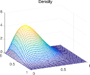
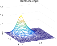
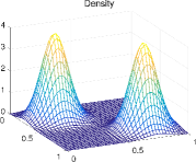
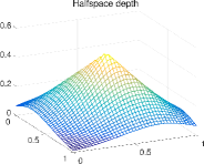
Figure 4: Illustration of the halfspace depth function. Mesh plot of the density and the halfspace depth function of a product of two $Beta(2,4)$-distributions (1st & 2nd plot) and a mixture of two Gaussians (3rd & 4th plot), respectively.

The first statistical depth function has been proposed by Tukey (1974). Given a probability distribution $P$ on $\mathbb{R}^{m}$, the seminal halfspace depth function $HD$ maps every point $x\in\mathbb{R}^{m}$ to the smallest probability of a closed halfspace containing $x$, that is

$$HD(x;P)=\inf_{u\in S^{m-1}}P(\{y\in\mathbb{R}^{m}:u^{T}(y-x)\geq 0\}),$$

where $S^{m-1}=\{u\in\mathbb{R}^{m}:u^{T}u=1\}$ denotes the unit sphere in $\mathbb{R}^{m}$. The intuition behind this definition is simplest to understand in case of an absolutely continuous distribution $P$: in this case $HD(x;P)\leq 1/2$, $x\in\mathbb{R}^{m}$, and in order for a point $x$ to be considered central with respect to $P$ it should hold that any hyperplane passing through $x$ splits $\mathbb{R}^{m}$ into two halfspaces of almost equal probability $1/2$. Hence, points $x$ are considered more central the higher their halfspace depth value $HD(x;P)$ is, and any point maximizing $HD({}\cdot{};P)$ is called a Tukey median. Figure 4 shows examples of the halfspace depth function for two absolutely continuous distributions on $\mathbb{R}^{2}$. Note that a depth function can resemble the density function of the underlying distribution only in case of a unimodal distribution—as a measure of global centrality depth functions are intended to be unimodal. We will take this up again in Section 6.1.2 and Section 7.

For a univariate and continuous distribution any ordinary median is also a Tukey median. In addition, the halfspace depth function $HD$ satisfies a number of desirable properties:

1. Affine invariance: $HD$ considered as a function in both $x$ and $P$ is invariant under affine transformations.

2. Maximality at the center: for a (halfspace) symmetric distribution the center of symmetry is a Tukey median.

3. Monotonicity with respect to the deepest point: if there is a unique Tukey median $\mu$, $HD(x;P)$ decreases as $x$ moves away along a ray from $\mu$.

4. Vanishing at infinity: $HD(x;P)\rightarrow 0$ as $\|x\|\rightarrow\infty$.

Even though there is not a unique definition of a statistical depth function, these or closely related properties are typically requested for a function to qualify as depth function. Beside Tukey’s halfspace depth, prominent examples of depth functions are simplicial depth (Liu, 1988, 1990), majority depth, projection depth, or Mahalanobis depth (Liu, 1992; Zuo and Serfling, 2000). To the best of our knowledge, the lens depth function (Liu and Modarres, 2011) is the only statistical depth function from the literature that can be evaluated given only ordinal distance information about a data set in an arbitrary semimetric space. Note that the function $F$ defined in (19), which the approach by Heikinheimo and Ukkonen (2013) is based on, is provably not a statistical depth function. It does not satisfy the property of maximality at the center for symmetric distributions. Indeed, as Heikinheimo and Ukkonen observe, in case of a symmetric bimodal distribution in one dimension with the two modes sufficiently far apart, the center of symmetry is in fact a minimizer of $F$.

We provide some references related to our Algorithms 2 and 3: The idea of considering data points with a small depth value as outliers has been thoroughly studied in the setting of a contamination model in Chen et al. (2009) and Dang and Serfling (2010). In particular, they deal with the question of determining what a small depth value is.

The simple max-depth approach to binary classification outlined in Section 3.1 has already been proposed by Liu (1990), using simplicial depth instead of the lens depth function. It has been theoretically studied in Ghosh and Chaudhuri (2005). Ghosh and Chaudhuri were able to prove that the max-depth approach is consistent, that is it asymptotically achieves Bayes risk, for equally probable and elliptically symmetric classes that only differ in location when using one of several depth functions and dealing with general $K$-class problems. Working not too well when these assumptions are not satisfied, the max-depth approach has been refined by Li et al. (2012) by allowing for more general classifiers on the DD-plot, thus overcoming some of its original limitations. The DD-plot (depth vs. depth plot; introduced by Liu et al., 1999) is the image of the data under the feature map $x\mapsto(DF(x;Class_{1}),DF(x;Class_{2}))\in\mathbb{R}^{2}$, where $DF$ denotes the depth function under consideration. Interestingly, Li et al. again only consider the 2-class case and propose a one-vs-one approach for the general case, which is different from our strategy of simply considering

$$x\mapsto(DF(x;Class_{1}),DF(x;Class_{2}),\ldots,DF(x;Class_{K}))\in\mathbb{R}^{K}$$

as feature map and subsequently performing classification on $\mathbb{R}^{K}$.

We conclude this section with some comments about the lens depth function. An early version of the lens depth function has already been mentioned, but not seriously studied, by Lawrence (1996, Section 2.3) and by Bartoszynski et al. (1997). The main reference for the lens depth function is Liu and Modarres (2011), where the lens depth function has been defined and systematically investigated. However, after reading the proofs in detail, we found that there is still an important gap. Liu and Modarres (2011) claim that the lens depth function satisfies the property of maximality at the center for centrally symmetric distributions on $\mathbb{R}^{m}$ (Theorem 6 in their paper). However, there is an error in their proof. It is not true that, conditioning on $X_{1}$, the probability of $X_{2}$ falling into a region such that $t\in Lens(X_{1},X_{2})$ holds decreases as $t\in\mathbb{R}^{m}$ moves away from the center for all values of $X_{1}$, and hence the monotonicity of the integral is not guaranteed. The same mistake appears in Elmore et al. (2006) and in Section 2.5 of Yang (2014) when showing the property for the spherical depth function and the $\beta$-skeleton depth function, respectively. So it has not yet been established that the lens depth function satisfies this essential property of statistical depth functions. We were not able to fix the proof, but we still believe that the statement is correct. At least, unlike for the function $F$ defined in (19), we have not been able to construct any example of a symmetric distribution for which the lens depth function does not attain its maximum at the center.

5.3 $k$-Relative Neighborhood Graph

The $k$-RNG belongs to the class of proximity graphs: two vertices are connected if they are in some sense close to each other (see Jaromczyk and Toussaint, 1992, for a basic survey or Bose et al., 2012, for a more recent paper). Beside the $k$-RNG, Gabriel graphs (Gabriel and Sokal, 1969) and $k$-NN graphs are prominent examples of proximity graphs.

The $1$-RNG, which is simply known as RNG, has been used in a wide range of applications (see Toussaint, 2014, for a review and detailed references). Most interesting for us are its use in classification and clustering as related to our Algorithms 4 and 5, respectively: Instance-based classification based on the RNG neighborhood, that is inferring a point’s label by taking a majority vote of the point’s neighbors in the RNG, has been empirically shown to be competitive with the $k$-NN classifier in Sánchez et al. (1997a) and Toussaint and Berzan (2012). Instance-based classification based on the RNG neighborhood has also been used for prototype selection for the $1$-NN classifier (Toussaint et al., 1984; Sánchez et al., 1997b). The RNG has been used for spectral clustering in Correa and Lindstrom (2012) with a strategy of assigning locally adapted edge weights. Our experiments in Section 6.1.4 show that such a strategy is dispensable and that using the $k$-RNG weighted as in (9), or also unweighted, yields reasonable results as well.

We have mentioned in Section 3.2 and Section 4.4 that a true $k$-RNG (not an estimated one) is always connected. This follows from the fact that the RNG on a data set ${\cal D}$ contains the minimal spanning tree on ${\cal D}$ as a subgraph. By minimal spanning tree we mean the minimal spanning tree of the complete graph on ${\cal D}$ in which an edge is weighted with the distance between two points. A proof of this property for data points in the Euclidean plane, which readily generalizes to data sets in arbitrary semimetric spaces, can be found in Toussaint (1980). The RNG is guaranteed to be sparse for data sets in the 2-dimensional or 3-dimensional Euclidean space, but it can be dense in higher-dimensional spaces or if $d$ is induced by the $1$-norm or the maximum norm (Jaromczyk and Toussaint, 1992). There is a large literature on the question how to efficiently compute a $k$-RNG on a data set, mainly for data sets in $\mathbb{R}^{2}$ or $\mathbb{R}^{3}$ (see the references in Toussaint, 2014), and how to approximate the RNG by a graph that is easier to compute (Andrade and de Figueiredo, 2001). We are not aware of any work that deals with estimating the $k$-RNG as we do in this paper.

6 Experiments

We performed several experiments for examining the performance of our proposed Algorithms 1 to 5 and compared them to ordinal embedding approaches. In case of Algorithm 1 and Algorithm 2 we also made a comparison with the methods proposed by Heikinheimo and Ukkonen (2013) explained in Section 5.1.1. Recall that an ordinal embedding approach consists of first constructing an ordinal embedding of a data set ${\cal D}$ based on the given ordinal distance information and then solving the problem on the embedding by applying a standard algorithm. For example, in the case of medoid estimation a medoid of an ordinal embedding is computed and the corresponding object is returned as an estimate of a medoid of ${\cal D}$. For constructing an ordinal embedding we tried several algorithms: the GNMDS (generalized non-metric multidimensional scaling) algorithm by Agarwal et al. (2007), the SOE (soft ordinal embedding) algorithm by Terada and von Luxburg (2014), and the STE (stochastic triplet embedding) and t-STE (t-distributed stochastic triplet embedding) algorithms by van der Maaten and Weinberger (2012). The GNMDS algorithm and the SOE algorithm can take answers to arbitrary dissimilarity comparisons of the form (17) as input, while the STE and t-STE algorithms are designed only for similarity triplets, that is answers to comparisons (18). The ordinal data that we gave to the embedding algorithms were all the similarity triplets obtained via (2) from a collection of statements of the kind ($\star$ ‣ 1) that we provided as input to one of our algorithms. We used the Matlab implementations of GNMDS, STE, and t-STE provided by van der Maaten and Weinberger (2012) and the R implementation of SOE provided by Terada and von Luxburg (2014). We set all parameters except the dimension $m$ of the space of the embedding to the provided default parameters (for all algorithms the default dimension is two). Note that all algorithms try to iteratively minimize an objective function that measures the amount of violated ordinal relationships, and in doing so their results depend on a random initialization of the ordinal embedding.

We start with presenting experiments on artificial data in Section 6.1. In Section 6.2 we deal with real data consisting of 60 images of cars and ordinal distance information of the kind ($\star$ ‣ 1) that we have collected via crowdsourcing in an online survey.

6.1 Artificial Data

In the following, except the plots in Figures 8 and 9, where outliers have to be identified by visual inspection, and one plot in Figure 5, which provides a visualization of available statements per data point, all plots of this section show results averaged over running the experiments for 100 times.

We primarily study the performance of the considered methods with respect to the number of provided input statements, but also with respect to the amount of noise in the provided ordinal data. We consider two different noise models: Noise model I (with parameter $0\leq errorprob\leq 1$) equals the one described in Section 3.2.1, that is a statement of the kind ($\star$ ‣ 1) is incorrect, independently of other statements, with some fixed error probability $errorprob$. In an incorrect statement the two data points that are not most central appear to be most central with probability $1/2$ each. In Noise model II (with parameter $noiseparam\geq 0$) we distort the dissimilarity values $d(A,B)$, which then induces a distortion of statements. Concretely, we add Gaussian noise with mean zero and standard deviation $noiseparam\cdot SD$, where $SD$ denotes the standard deviation of all true dissimilarity values $d(A,B)$, $A\neq B\in{\cal D}$, independently to each dissimilarity value $d(A,B)$. For choosing input statements we essentially consider two sampling strategies: The first one, referred to as uniform sampling, is to choose input statements uniformly at random without replacement from the set of all statements, that is the set of statements for all triples of data points, which were generated according to the noise model under consideration. When applying this sampling strategy and studying performance as a function of the number of input statements, the rightmost measurement in a plot corresponds to the case that all statements are provided as input. In the experiment presented in Figure 7 the provided statements are chosen uniformly at random with replacement from the set of all statements, but there the set of all statements is so large that in fact this does not make any difference. In these plots the rightmost measurement corresponds to a number of input statements of less than one permil of the number of all statements. In order to illustrate our claim that our algorithms require statements to be sampled only approximately uniformly with respect to a fixed data point (Algorithms 1 to 3), or a fixed pair of data points (Algorithms 4 and 5), we also consider a second sampling strategy, referred to as Sampling II. When sampling according to this strategy, we partition the data set into ten groups. For each group we form a set consisting of all statements, generated according to the noise model under consideration, that comprise at least one data point from the corresponding group. We then sample with replacement by selecting one of the ten sets according to probabilities $i^{2}/\sum_{j=1}^{10}j^{2}$, $i=1,\ldots,10$, and choosing a statement from the selected set uniformly at random.

When comparing Algorithm 1 or Algorithm 2 to the corresponding methods by Heikinheimo and Ukkonen (2013) in Sections 6.1.1 and 6.1.2, their methods are given a collection of statements of the kind ($\boxplus$ ‣ 1) as input that contains as many statements as the input to our algorithm and is created in a completely analogous way.

Uniform sampling	Noise model I	Relative error
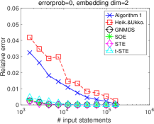
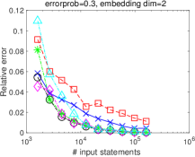
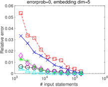
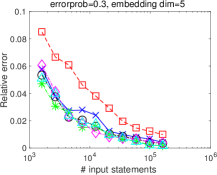
				\begin{overpic}[height=91.04872pt]{Pictures/Median_experiments/withTIME_AVERAGE100_2dimGauss_100points_EucMetric/includingSTE/Func_of_error/Median_FofErProb_01gauss2dim_100points_NrTri25_embeddim2_CUT} \put(6.0,16.0){\includegraphics[height=31.86694pt]{Pictures/Median_experiments/withTIME_AVERAGE100_2dimGauss_100points_EucMetric/includingSTE/Func_of_error/INLAY_Median_FofErProb_01gauss2dim_100points_NrTri25_embeddim2_CUT}} \end{overpic}	\begin{overpic}[height=91.04872pt]{Pictures/Median_experiments/withTIME_AVERAGE100_2dimGauss_100points_EucMetric/includingSTE/Func_of_error/Median_FofErProb_01gauss2dim_100points_NrTriALL_embeddim2_CUT} \put(6.0,16.0){\includegraphics[height=31.86694pt]{Pictures/Median_experiments/withTIME_AVERAGE100_2dimGauss_100points_EucMetric/includingSTE/Func_of_error/INLAY_Median_FofErProb_01gauss2dim_100points_NrTriALL_embeddim2_CUT}} \end{overpic}
		Running time
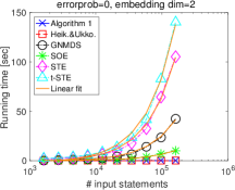
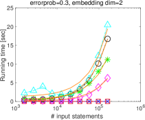
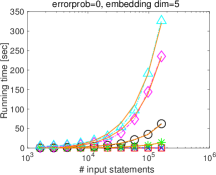
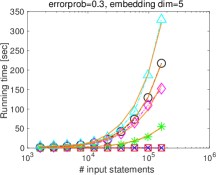
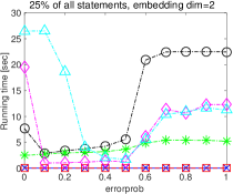
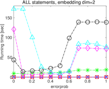
Sampling II		Rel. error / sampling

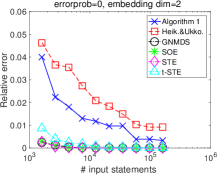
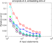
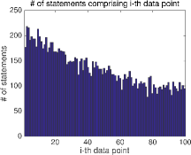
Figure 5: Medoid estimation — $100$ points from a $2$-dim Gaussian $N_{2}(0,I_{2})$ with Euclidean metric. Relative error (20) and running time as a function of the number of provided statements of the kind ($\star$ ‣ 1) or of the kind ($\boxplus$ ‣ 1) and as a function of $errorprob$ for Algorithm 1, for the method by Heikinheimo and Ukkonen, and for the embedding approach using the various embedding methods.

6.1.1 Medoid Estimation

We measure performance of a method for medoid estimation by the relative error in the objective $D$ (given in (6)), which is given by

$$\text{relative error}=\frac{D(\text{estimated medoid})-D(\text{true medoid})}{D(\text{true medoid})}.$$ (20)

Figure 5 shows in the first two rows the relative error of Algorithm 1, the method by Heikinheimo and Ukkonen (2013), and the embedding approach, using the various embedding algorithms, as a function of the number of provided input statements and as a function of $errorprob$ (Noise model I) for $100$ points from a $2$-dimensional Gaussian $N_{2}(0,I_{2})$ and $d$ being the Euclidean metric. Obviously, the embedding approach outperforms Algorithm 1 and the method by Heikinheimo and Ukkonen when dealing only with correct statements, that is $errorprob=0$, and embedding into the true dimension (1st row, 1st plot). However, it is not superior over Algorithm 1 anymore when $errorprob=0.3$ and the dimension of the embedding is chosen as five (2nd row, 1st plot). Algorithm 1 consistently outperforms the method by Heikinheimo and Ukkonen. All methods show a similar behavior with respect to $errorprob$ (2nd row, 2nd & 3rd plot). Interestingly, the strongest incline in the error does not occur until the transition from $errorprob=0.6$ to $errorprob=0.7$. The bottom row of Figure 5 also shows the relative error of the various methods as a function of the number of provided input statements, but here input statements were sampled according to the strategy Sampling II. Compared to the strategy of sampling statements uniformly at random without replacement from the set of all statements, Algorithm 1 performs slightly worse, but we consider the difference to be negligible. The last plot of the bottom row shows the difference in the two sampling strategies: while in the uniform case, for all data points there is almost the same number of input statements comprising the data point, when sampling according to Sampling II there are data points for which this number is twice as large as for others (the plot is based on a total of 4500 input statements corresponding to the third measurement in the first and second plot of the bottom row).

Uniform sampling

Noise model I

Relative error

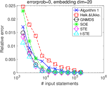
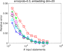
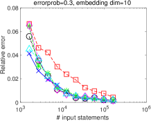
Figure 6: Medoid estimation — $100$ points from a $20$-dim Gaussian $N_{20}(0,I_{20})$ with Euclidean metric. Relative error (20) as a function of the number of provided statements of the kind ($\star$ ‣ 1) or of the kind ($\boxplus$ ‣ 1) for Algorithm 1, for the method by Heikinheimo and Ukkonen, and for the embedding approach using the various embedding methods.

The biggest advantage of Algorithm 1 (in fact of all our proposed algorithms) compared to an ordinal embedding approach becomes obvious from the plots in the third and fourth row of Figure 5, which show the running times of the experiments shown in the plots in the two top rows: For a fixed size $|{\cal D}|$ of the data set, like the running times of our proposed algorithms and the method by Heikinheimo and Ukkonen, the running time of the embedding approach with any of the considered embedding algorithms also grows linearly with the number $|\mathcal{S}|$ of input statements (indicated by the orange curves). However, in practice Algorithm 1 and the method by Heikinheimo and Ukkonen are vastly superior in terms of running time compared to the embedding approach, even without making use of their potential of simple and highly efficient parallelization. For example, when all statements are provided as input, $errorprob=0$, and the embedding dimension is chosen as two, the running time of the embedding approach is between 10 seconds (when using the SOE algorithm) and 141 seconds (when using the t-STE algorithm), while Algorithm 1 or the method by Heikinheimo and Ukkonen only run for 0.01 seconds (3rd row, 1st plot). Note that the running times of Algorithm 1 and the method by Heikinheimo and Ukkonen are independent of $errorprob$ and, of course, of the choice of a dimension of the space of the embedding. The running times of the embedding algorithms tend to increase with the embedding dimension (e.g., differences between the first and the third plot in the third row). The running time of the SOE algorithm also increases with $errorprob$ (4th row, 2nd & 3rd plot). For the GNMDS algorithm this holds for $errorprob\geq 0.1$. The running times of the STE and t-STE algorithms vary non-monotonically with $errorprob$. All experiments shown in Figure 5 were performed in Matlab R2015a on a MacBook Pro with 2.6 GHz Intel Core i7 and 8 GB 1600 MHz DDR3. Within Matlab we invoked R 3.2.2 for computing the SOE embedding. In order to make a fair comparison we did not use MEX files in the implementation of Algorithm 1 or the method by Heikinheimo and Ukkonen.

Unif. sampling WR

Noise model I

Relative error / running time

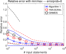
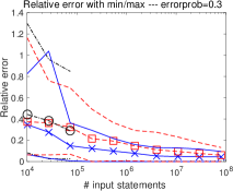
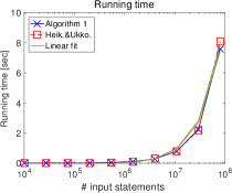
Figure 7: Medoid estimation — $8638$ vertices in a collaboration network with shortest-path-distance. 1st & 2nd plot: Relative error (20) as a function of the number of provided statements of the kind ($\star$ ‣ 1) or of the kind ($\boxplus$ ‣ 1) for Algorithm 1, for the method by Heikinheimo and Ukkonen, and for the embedding approach using GNMDS (for the first three measurements). Average over 100 runs together with the minimum and the maximum of the 100 runs. 3rd plot: The corresponding running times with fitted linear functions.

Figure 6 shows almost the same experiments as Figure 5, but this time dealing with $100$ points from a $20$-dimensional Gaussian $N_{20}(0,I_{20})$. The distance function $d$ again equals the Euclidean metric. In this high-dimensional case the embedding approach cannot be considered superior anymore. In fact, when $errorprob=0.3$ and the number of input statements is small, Algorithm 1 performs best (2nd plot). We omit to show plots of the relative error as a function of $errorprob$ since they look very similar to the ones in Figure 5. Time measurements show that the differences in running times between the embedding approach and Algorithm 1 or the method by Heikinheimo and Ukkonen are even more severe compared to Figure 5, as to be expected because of the high embedding dimensions (plots omitted).

Finally, we applied Algorithm 1 and the method by Heikinheimo and Ukkonen to a large network with the dissimilarity function $d$ equaling the shortest-path-distance. In this context, a medoid is usually referred to as a “most central point with respect to the closeness centrality measure” (Freeman, 1978). Our data set consists of 8638 vertices, which form the largest connected component of a collaboration network with 9877 vertices that represent authors of papers submitted to arXiv in the High Energy Physics - Theory category and with two vertices being connected if the authors co-authored at least one paper (Leskovec et al., 2007). Comparing against the embedding methods as in the previous experiments on this large data set would have taken months (considering various numbers of input statements and averaging over 100 runs), so we only compared against GNMDS (embedding dimension chosen to equal two) for a small number of input statements. The first and the second plot of Figure 7 show the relative error of Algorithm 1 and the method by Heikinheimo and Ukkonen as a function of the number of provided statements of the kind ($\star$ ‣ 1) or of the kind ($\boxplus$ ‣ 1). The number of provided statements varies between $10^{4}$ and $8\cdot 10^{7}$. The latter is less than one permil of the number of all statements, which is $\tbinom{8638}{3}\approx 10^{11}$. This number is so large that the set of all statements does by no means fit into the main memory of a single machine. The plots also show the relative error of the embedding approach using the GNMDS algorithm for 10000, 27144, and 73680 input statements. As in the previous experiments, the shown error is the average over 100 runs of the experiment, but here the data set is fixed and the only sort of randomness comes from the input statements (and the random initialization of the ordinal embedding in case of GNMDS). In addition to the average error the plots show the minimum and maximum error of the 100 runs for illustrating the variance in the methods. In both the cases of $errorprob=0$ (1st plot) and $errorprob=0.3$ (2nd plot), when the number of input statements is small, Algorithm 1 outperforms the method by Heikinheimo and Ukkonen. Both methods outperform the embedding approach, which might have difficulties due to the data set being non-Euclidean or might struggle with a too small embedding dimension. For comparison, a strategy of choosing a data point uniformly at random as medoid estimate incurs a relative error of $0.47$ in expectation. Even when given only $10000$ input statements, when $errorprob=0$, the error of Algorithm 1 is only about one half of this. The variance seems to be similar for both Algorithm 1 and the method by Heikinheimo and Ukkonen and seems to be significantly larger for the embedding approach. As expected, it decreases as the number of input statements increases. In case of $errorprob=0$, we also applied GNMDS to the data set providing 10857670 statements as input (corresponding to the eighth measurement in the plots): averaging over 10 runs we obtained an average relative error of 0.28 (which is more than six times larger than the error of Algorithm 1 or the method by Heikinheimo and Ukkonen), where computation took 2.84 hours on average. The third plot of Figure 7 shows the running times of Algorithm 1 and the method by Heikinheimo and Ukkonen as a function of the number of input statements. Both methods have the same running time, which is linear in the number of input statements. The plot does not show the running times of GNMDS at the first three measurements. These were 110, 860, and 879 seconds in case of $errorprob=0$ and 92, 848, and 898 seconds in case of $errorprob=0.3$.

6.1.2 Outlier Identification

Uniform sampling	Noise model I	Point cloud / sorted values

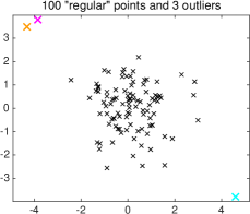
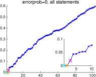
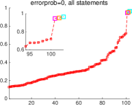
Figure 8: Outlier identification — $100$ points from a $2$-dim Gaussian $N_{2}(0,I_{2})$ and three outliers added by hand with Euclidean metric. Data set and sorted values of $LD(O)$ as needed for Algorithm 2 (left; in blue) and of estimated probabilities as needed for the method by Heikinheimo and Ukkonen (right; in red).

Uniform sampling	Noise model I	Point cloud / sorted values

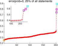
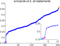
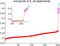
Figure 9: Outlier identification — $200$ points from a Two-moons data set and four outliers added by hand with Euclidean metric. Data set and sorted values of $LD(O)$ as needed for Algorithm 2 (left; in blue) and of estimated probabilities as needed for the method by Heikinheimo and Ukkonen (right; in red).

We started with testing Algorithm 2 and the corresponding method by Heikinheimo and Ukkonen (2013) by applying them to two visualizable data sets containing some obvious outliers. Both of the Figures 8 and 9 show a scatterplot of the points of a data set ${\cal D}$ in the Euclidean plane with the “regular” points in black and the outliers in color. For assessing the performance of the two considered methods we plotted the sorted values of $LD(O)$, $O\in{\cal D}$, as needed for Algorithm 2 as well as the sorted values of estimated probabilities of being an outlier within a triple of objects as needed for the method by Heikinheimo and Ukkonen (compare with Section 5.1.1). Both methods were provided with the same number of statements as input, either of the kind ($\star$ ‣ 1) or of the kind ($\boxplus$ ‣ 1). Both Figure 8 and Figure 9 provide several such plots, varying with this number of input statements as well as with the error probability $errorprob$ (we generated statements according to Noise model I). In all the plots, values belonging to outliers have the same color as the corresponding outlier in the scatterplot. The methods are successful if these colored values appear at the very end of the sorted values, either at the lower end for Algorithm 2 or at the upper end for the method by Heikinheimo and Ukkonen, and there is a (preferably large) gap between the colored values and the remaining ones since then it is easy to correctly identify the outliers. There are inlay plots showing the bottom or top ten values for more precise inspection. Note that there is no averaging involved in creating these plots and they may change with every run of the experiment since they depend on the random data set, the random choice of statements that are provided as input, and the random occurrence of incorrect statements.

In Figure 8 the data set consists of 100 points that were drawn from a 2-dimensional Gaussian $N_{2}(0,I_{2})$ and three outliers added by hand. The dissimilarity function $d$ equals the Euclidean metric. We can see that for both methods the values corresponding to the outliers appear at the right place when given all correct statements as input (top row). However, when given only 25 percent of all statements and $errorprob=0.3$, for Algorithm 2 the estimated lens depth value of the pink outlier ranks only sixth smallest, and thus this outlier might not be identified (bottom left). Furthermore, even in the previous situation it might not be possible to correctly infer the number of outliers based on the plot corresponding to Algorithm 2 due to the lack of a clear gap, whereas in both situations this can easily be done for the method by Heikinheimo and Ukkonen. We made similar observations for smaller numbers of provided input statements and other values of $errorprob$ too (plots omitted).

Uniform sampling	Noise model I	# correctly identified
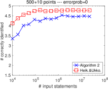
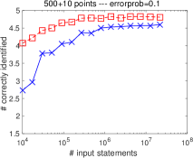
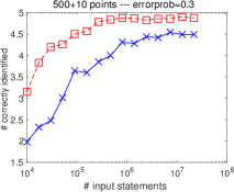
Sampling II	Noise model II

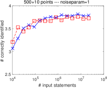
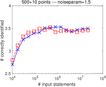
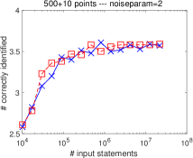
Figure 10: Outlier identification — $500$ points from the subset of USPS digits $6$ and ten outlier digits with Euclidean metric. Number of correctly ranked outliers as a function of the number of provided statements of the kind ($\star$ ‣ 1) or of the kind ($\boxplus$ ‣ 1) for Algorithm 2 and for the method by Heikinheimo and Ukkonen.

In Figure 9 the data set consists of 200 points from a Two-moons data set and four outliers added by hand. Again, $d$ equals the Euclidean metric. Both methods correctly identify the three outliers located quite far apart from the bulk of the data points, and the gap between their values and values belonging to the “regular” data points is large enough to be easily spotted. However, both methods fail to identify the outlier located in-between the two moons (yellow point). The estimated lens depth values or probabilities indicate that this outlier might be the unique medoid—which is indeed the case. For Algorithm 2 this has to be expected and stresses the inherent property of the lens depth function, and statistical depth functions in general, of globally measuring centrality. In doing so, it ignores multimodal aspects of the data (compare with Section 5.2 and Section 7) and cannot be used for identifying outliers that are globally seen at the heart of a data set. At least for the data set of Figure 9 this also holds for the function $F$ defined in (19), which the method by Heikinheimo and Ukkonen is based on. However, for the function $F$ this behavior is not systematic as the example of a symmetric bimodal distribution in one dimension as mentioned in Section 5.2 shows.

In the last experiment of this section we study Algorithm 2 and the method by Heikinheimo and Ukkonen by using them for outlier identification in a data set consisting of USPS digits. The data set consists of $500$ digits chosen uniformly at random from digits $6$ and ten outlier digits chosen uniformly at random from the remaining digits. The dissimilarity function $d$ equals the Euclidean metric. We assess the performance of Algorithm 2 and the method by Heikinheimo and Ukkonen by counting how many of the ten outliers are among the ten digits ranked lowest or highest according to the values of $LD(O)$ and estimated probabilities, respectively. Figure 10 shows these numbers as a function of the number of provided input statements in case of uniform sampling and statements generated according to Noise model I (1st row) and in case of Sampling II and statements generated according to Noise model II (2nd row), for $errorprob=0$ / $noiseparam=1$ (1st plot), $errorprob=0.1$ / $noiseparam=1.5$ (2nd plot), and $errorprob=0.3$ / $noiseparam=2$ (3rd plot). We can see that the method by Heikinheimo and Ukkonen performs slightly better in the setting of the first row and that the performance of both methods is essentially the same in the setting of the second row. Most often, the methods can identify three to five outliers, which we consider to be not bad, but not good either. Choosing another digit than $6$ for defining the bulk of “regular” points leads to similar results (plots omitted).

To sum up the insights from the experiments shown in Figures 8 to 10, we may conclude that both methods are capable of identifying outliers located lonely and far apart from the bulk of a data set, but should be used with some care in general. The method by Heikinheimo and Ukkonen seems to be superior—which is not very surprising since statements of the kind ($\boxplus$ ‣ 1) readily inform about outliers within triples of data points. It produces larger and thus easier to spot gaps than Algorithm 2, but is less understood theoretically.

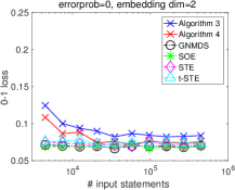
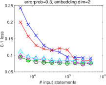
Uniform sampling	Noise model I	0-1 loss			\begin{overpic}[height=91.04872pt]{Pictures/Classification_experiments/Two_Gaussians_100l+40ulPoints/including_STE/FINAL_AVER100FuncOfError_01loss_2dimMixGauss_Lp100_ULp40_Ntri25_embeddim2_kfold10_nloo20_withSTE_CUT} \put(6.0,16.0){\includegraphics[height=31.86694pt]{Pictures/Classification_experiments/Two_Gaussians_100l+40ulPoints/including_STE/inlay_func_of_error_25percent_CUT}} \end{overpic}
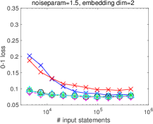
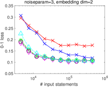
	Noise model II				\begin{overpic}[height=91.04872pt]{Pictures/Classification_experiments/NEW_NOISE_Two_Gaussians_100l+40ulPoints/NEWERROR2_AVER100_FuncOfError_Ntri25_embeddim2_CUT} \put(7.0,16.0){\includegraphics[height=31.86694pt]{Pictures/Classification_experiments/NEW_NOISE_Two_Gaussians_100l+40ulPoints/NEWERROR2_AVER100_FuncOfError_Ntri25_embeddim2_ausschnitt_CUT}} \end{overpic}
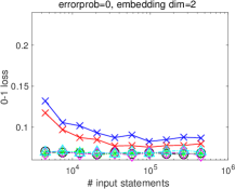
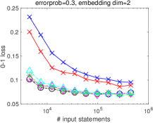
Sampling II	Noise model I				\begin{overpic}[height=91.04872pt]{Pictures/Classification_experiments/NEW_SAMPLING_Two_Gaussians_100l+40ulPoints/newsampl_aver100_FuncOfError_CUT.pdf} \put(4.0,16.0){\includegraphics[height=31.86694pt]{Pictures/Classification_experiments/NEW_SAMPLING_Two_Gaussians_100l+40ulPoints/newsampl_aver100_FuncOfError_Inlay_CUT}} \end{overpic}

Figure 11: Classification — 100 labeled and 40 unlabeled points from a mixture of two equally probable 2-dim Gaussians $N_{2}(0,I_{2})$ and $N_{2}((3,0)^{T},I_{2})$ with Euclidean metric. SVM algorithm with linear kernel on top of Algorithm 3 as well as on the embedding approach. 0-1 loss (21) as a function of the number of provided statements of the kind ($\star$ ‣ 1) and as a function of $errorprob$ / $noiseparam$ for Algorithm 3, for Algorithm 4, and for the embedding approach using the various embedding methods.

6.1.3 Classification

We compared Algorithms 3 and 4 to an ordinal embedding approach that consists of embedding a data set ${\cal D}$ comprising a set $\mathcal{L}$ of labeled data points and a set $\mathcal{U}$ of unlabeled data points into $\mathbb{R}^{m}$ using the given ordinal distance information and applying a classification algorithm to the embedding. Note that this approach is semi-supervised since it makes use of answers to dissimilarity comparisons involving data points of $\mathcal{U}$ for constructing the embedding of ${\cal D}$. Algorithm 3, in contrast, only uses ordinal distance information involving data points of $\mathcal{L}$ for approximately evaluating the feature map (7) on $\mathcal{L}$ and hence is a supervised technique as long as the classifier on top is. Algorithm 4 is a supervised instance-based learning method. Algorithm 3 as well as the embedding approach require an ordinary classifier on top, that is a classifier appropriate for real-valued feature vectors. For simplicity, in the experiments presented here we either used the $k$-NN classifier or the SVM (support vector machine) algorithm with the standard linear kernel (e.g., Cristianini and Shawe-Taylor, 2000). Both these classification algorithms require to set parameters, which we did by means of 10-fold cross-validation: the parameter $k$ for the $k$-NN classifier was chosen from the range $1,3,5,7,11,15,23$ and the regularization parameter for the SVM algorithm was chosen from $0.01,0.05,0.1,0.5,1,5,10,50,100,500,1000$. The ordinal embedding algorithms produce embeddings on an arbitrary scale. Before applying the classification algorithms, we rescaled an ordinal embedding to have diameter 2. The feature embedding constructed by Algorithm 3 always resides in $[0,1]^{K}$ for a $K$-class classification problem and no rescaling was done here. Algorithm 4 requires to set the parameter $k$ describing which $k$-RNG it is based on, but this is more subtle: As we have seen in Section 3.2.1, when input statements are incorrect with some error probability $errorprob>0$ (Noise model I), then our estimation strategy does not estimate the $k$-RNG anymore, but rather a $k^{\prime}$-RNG with $k^{\prime}=k^{\prime}(k,errorprob,|{\cal D}|)$ depending on the size of the data set as given in (15). We thus have to choose the range of possible values for the parameter $k$ in Algorithm 4 depending on $|{\cal D}|$. Furthermore, we cannot use 10-fold cross-validation for choosing the best value within this range since, roughly speaking, this would lead to choosing the best parameter for a data set of size of only 90 percent of $|{\cal D}|$. Instead, we used a non-exhaustive variant of leave-one-out cross-validation: we randomly selected a single training point as validation set and repeated this procedure for 20 times, and finally chose the parameter that showed the best performance on average.

Uniform sampling	Noise model I	0-1 loss
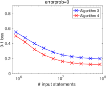
	Noise model II

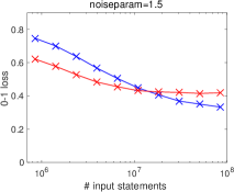
Figure 12: Classification — 300 labeled and 500 unlabeled USPS digits with Euclidean metric. $k$-NN classifier on top of Algorithm 3. 0-1 loss (21) as a function of the number of provided statements of the kind ($\star$ ‣ 1) for Algorithm 3 and for Algorithm 4.

We measure performance of Algorithms 3 and 4 and the embedding approach by considering their incurred 0-1 loss given by

$$\text{0-1 loss}=\frac{1}{|\mathcal{U}|}\cdot\sum_{O\in\mathcal{U}}\mathbb{1}\{\text{predicted label}(O)\neq\text{true label}(O)\}.$$ (21)

Figure 11 shows the results for a data set consisting of 100 labeled and 40 unlabeled points from a mixture of two equally probable 2-dimensional Gaussians $N_{2}(0,I_{2})$ and $N_{2}((3,0)^{T},I_{2})$ and $d$ being the Euclidean metric. True class labels of the points correspond to which Gaussian they come from. On top of Algorithm 3 as well as on the embedding methods we used the SVM algorithm with the linear kernel. The parameter $k$ for Algorithm 4 was chosen from the range $1,2,3,5,7,15,25,45,70$. The dimension of the space of the ordinal embedding was chosen to equal the true dimension two, but we observed similar results when we chose it as five instead (plots omitted). The embedding approach outperforms both Algorithm 3 and Algorithm 4, but their results appear to be acceptable too. Interestingly, other than for Algorithm 4 and the embedding approach, the 0-1 loss incurred by Algorithm 3 studied as a function of $errorprob$ (1st & 3rd row, 3rd plot) increases only up to $errorprob=0.7$ and then drops again, finally yielding almost the same result for $errorprob=1$ as for $errorprob=0$. In hindsight, this is not surprising: If $errorprob=1$, and thus every statement is incorrect, and the two possibilities of an incorrect statement are equally likely, as it is the case under Noise model I, then Algorithm 3 approximately evaluates the feature map

$$x\mapsto\left(\frac{1}{2}-\frac{1}{2}LD(x;Class_{1}),\frac{1}{2}-\frac{1}{2}LD(x;Class_{2}),\ldots,\frac{1}{2}-\frac{1}{2}LD(x;Class_{K})\right)\in\mathbb{R}^{K}.$$

This feature map coincides with the original one given in (7) up to a similarity transformation and hence gives rise to the same classification results.

In Figure 12 we study the performance of Algorithms 3 and 4 when used for classifying USPS digits. We deal with 800 digits chosen uniformly at random from the set of all USPS digits and randomly split into 300 labeled and 500 unlabeled data points. The dissimilarity function $d$ equals the Euclidean metric. We chose input statements uniformly at random without replacement from the set of all statements, which we generated according to Noise model I (1st row) or Noise model II (2nd row). On top of Algorithm 3 we used the $k$-NN classifier. The parameter $k$ for Algorithm 4 was chosen from $1,2,3,5,7,15,25,45,70,100,150,230,350$. For small values of $errorprob$ or $noiseparam$ we consider the results of our proposed algorithms to be satisfactory and useful. Note that in this 10-class classification problem a strategy of random guessing would yield a 0-1 loss of about $0.9$. Not surprisingly, we obtained slightly better results when the ratio between labeled and unlabeled data points was chosen as $400/400$ instead of $300/500$ and slightly worse results when it was chosen as $200/600$ (plots omitted).

6.1.4 Clustering

We compared Algorithm 5, both in its weighted and in its unweighted version, to an embedding approach in which we applied spectral clustering to a symmetric $k$-NN graph on an ordinal embedding of a data set ${\cal D}$. We put Gaussian weights $\exp(-\|u_{i}-u_{j}\|^{2}/\sigma^{2})$, where $u_{i}$ and $u_{j}$ are connected points of the embedding and $\sigma>0$ is a scaling parameter, on the edges of this $k$-NN graph. Again, we rescaled an ordinal embedding to have diameter 2. Both in Algorithm 5 and in the ordinal embedding approach we used the normalized version of spectral clustering as stated in von Luxburg (2007) and invented by Shi and Malik (2000). For assessing the quality of a clustering we measure its purity with respect to a ground truth partitioning of the data set ${\cal D}$ (e.g., Manning et al., 2008, Chapter 16): if ${\cal D}$ consists of $L$ different classes $C_{1},\ldots,C_{L}$ that we would like to recover and the clustering $\mathcal{C}$ comprises $K$ different clusters $U_{1},\ldots,U_{K}$, then the purity of $\mathcal{C}$ is given by

$$\text{purity}(\mathcal{C})=\text{purity}(\mathcal{C};{\cal D})=\frac{1}{|{\cal D}|}\sum_{k=1}^{K}\max_{l=1,\ldots,L}|U_{k}\cap C_{l}|.$$ (22)

We always have $K/|{\cal D}|\leq\text{purity}(\mathcal{C})\leq 1$, and a high value indicates a good clustering. In the experiments presented in this section, we always provided Algorithm 5 and the embedding approach with the correct number $L$ of clusters as input.

Uniform sampling

Noise model I

Purity

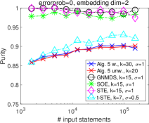
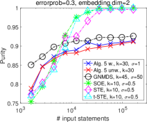
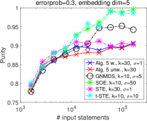
Figure 13: Clustering — 100 points from a uniform distribution on two equally sized moons in $\mathbb{R}^{2}$ with Euclidean metric. Purity (22) as a function of the number of provided statements of the kind ($\star$ ‣ 1) for Algorithm 5 in its weighted and unweighted version and for the embedding approach using the various embedding methods.

Figure 13 shows the purity of the clusterings produced by Algorithm 5 and the embedding approach when applied to a data set consisting of 100 points from a uniform distribution on two equally sized moons in $\mathbb{R}^{2}$. The two moons correspond to a ground truth partitioning into two classes. The dissimilarity function $d$ equals the Euclidean metric. The curves shown here are the results obtained by a particular choice of input parameters $k$ and $\sigma$: within a reasonably large range of parameter configurations this choice of parameters yielded the best performance on average with respect to the number of input statements. We study the sensitivity of Algorithm 5 with respect to the parameters in another experiment (shown in Figure 14). The embedding approach clearly outperforms Algorithm 5 if $errorprob=0$ (1st plot), where three of the considered embedding algorithms achieve significantly higher purity values over the whole range of the number of input statements. However, given the numerous advantages common to all our proposed algorithms compared to an ordinal embedding approach, we consider the performance of Algorithm 5 to be acceptable. For comparison, a random clustering in which data points are randomly assigned to one of two clusters independently of each other with probability one half has an average purity of $0.54$. If $errorprob=0.3$, the embedding approach is superior to Algorithm 5 only if the number of input statements is large. Interestingly, there is almost no difference in the performance of the weighted and the unweighted version of Algorithm 5.

Uniform sampling	Noise model I	Purity

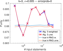
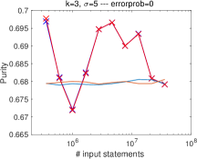
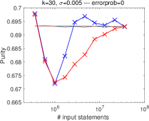
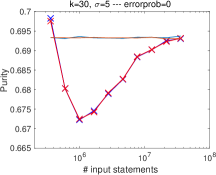
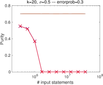
Figure 14: Clustering — 600 USPS digits with Euclidean metric. Purity (22) as a function of the number of provided statements of the kind ($\star$ ‣ 1) for Algorithm 5 in its weighted and unweighted version. The light blue curve and the bronze curve show the purity of the clusterings obtained by applying spectral clustering to the true weighted and unweighted $k$-RNG on the data set.

The experiment shown in Figure 14 deals with a data set ${\cal D}$ consisting of 600 digits chosen uniformly at random from the set of all USPS digits and $d$ being the Euclidean metric. We assume a ground truth partitioning of ${\cal D}$ into ten classes according to the digits’ values. For various parameter configurations the plots show the purity of the clusterings produced by the weighted (in blue) and unweighted (in red) version of Algorithm 5 as a function of the number of input statements. The plots also show the purity of the clusterings obtained when applying spectral clustering to the true weighted (in light blue) and unweighted (in bronze) $k$-RNG on ${\cal D}$. Note that these two curves only vary with the number of input statements because of random effects in the $K$-means step of spectral clustering. Although it might look odd at a first glance that the purity achieved by Algorithm 5 is not monotonic with respect to the number of input statements, we can see that the purity is always between $0.67$ and $0.7$ for a wide range of values of $k$ and $\sigma$ when $errorprob=0$ (1st row; 2nd row, 1st plot). For comparison, a random clustering in which data points are randomly assigned to one of ten clusters independently of each other with probability one-tenth has an average purity of $0.19$. A clustering obtained by applying spectral clustering to a symmetric $k$-NN graph with Gaussian edge weights $\exp(-d(x_{i},x_{j})^{2}/\sigma^{2})$ on ${\cal D}$ (the true data set—not an ordinal embedding) has an average purity of not higher than $0.75$, even for a good choice of $k$ and $\sigma$. When $errorprob=0.3$, Algorithm 5 completely fails for small values of $k$ (2nd row, 2nd plot) as has to be expected because of our findings in Section 3.2.1. For $k$ sufficiently large it finally yields the same purity values as when $errorprob=0$ (2nd row, 3rd plot). In fact, this is true already for $k=100$ and a wide range of values of $\sigma$ (plots omitted). Again, both in the case of $errorprob=0$ and in the case of $errorprob=0.3$, there is almost no difference in the performance of the weighted and the unweighted version of Algorithm 5.

\begin{overpic}[scale={1}]{Pictures/Cars/car_pictures_collectionCUT_compressed.pdf} \put(-0.35,54.5){\framebox{\begin{minipage}[c][0.8cm][c]{938.94093pt} \phantom{dddddddddddddddwwww} \end{minipage}}} \end{overpic}

Figure 15: Car data set. We collected ordinal distance information of the kind ($\star$ ‣ 1) for this data set via an online survey. The framed triple in the first row was used as a test case: T_All and T_All_reduced comprise only statements provided by participants that chose the off-road vehicle as the most central car in this triple. The pictures were found on Wikimedia Commons and have been explicitly released into the public domain by their authors.

6.2 Real Data

We set up an online survey for collecting ordinal distance information of the kind ($\star$ ‣ 1) for $60$ images of cars, shown in Figure 15. All images were found on Wikimedia Commons (https://commons.wikimedia.org) and have been explicitly released into the public domain by their authors. We refer to the set of these images as the car data set. We instructed participants of the survey to determine the most central object within a triple of three shown images according to how they perceive dissimilarity between cars. We explicitly stated that they should not judge differences between the pictures, like perspective, lighting conditions, or background. Every participant was shown triples of cars in random order (more precisely, triples shown to a participant were drawn uniformly at random without replacement from the set of all possible triples). Also the order of cars within a triple, that is whether a car’s image appeared to the left, in the middle, or to the right, was random. One complete round of the survey consisted of 50 shown triples, but we encouraged participants to contribute more than one round, possibly at a later time. There was no possibility of skipping triples, that is even if a participant had no idea which car might be the most central one in a triple, he/she had to make a choice—or quit the current round of the survey. Within the first ten triples every participant was shown a test case triple (shown within a frame in Figure 15), consisting of an off-road vehicle, a sports car, and a fire truck. We believe the off-road vehicle to be the obvious most central car in this triple and used this test case for checking whether a participant might have got the task of choosing a most central object correctly.

	All	All_reduced	T_All	T_All_reduced
Number of statements	7097	6338	6757	6056
Number of statements in percent of number of triples [$\tbinom{60}{3}=34220]$	20.74	18.52	19.75	17.70
Average number of statements in which a car appears	354.85	316.90	337.85	302.80
Minimum number of statements in which a car appears	307	286	292	269
Maximum number of statements in which a car appears	503	347	478	333
Median response time per shown triple (in seconds)	4.02	reNTE-1tNTE-1lNTE-1r	4.15	reNTE-2tNTE-2lNTE-2r

Table 1: Characteristic values of All, All_reduced, T_All, and T_All_reduced. Note that All and T_All contain repeatedly present and contradicting statements.

The survey was online for about two months and the link to the survey was distributed among colleagues and friends. We took no account of rounds of the survey that were quitted before 30 triples (of the fifty per round) were shown. In doing so, we ended up with 146 rounds (some of them not fully completed) and a total of 7097 statements. It is hard to guess how many different people contributed to these 146 rounds, but assuming an average of three to four rounds per person, which seems to be reasonable according to personal feedback, their number should be around 40. In only 7 out of the 146 rounds the off-road vehicle was not chosen as most central car in the test case triple. We refer to the collection of the total of 7097 statements as the collection All and to its subcollection comprising 6757 statements gathered in the 139 rounds in which the off-road vehicle was chosen as most central car in the test case triple as the collection T_All. From All and T_All we derived two more collections of statements of the kind ($\star$ ‣ 1) for the car data set as follows: All_reduced is obtained from All by replacing all statements dealing with the same triple of cars by just one statement about this triple, with the most central car being that car that is most often the most central car in the statements to be replaced. T_All_reduced is derived from T_All analogously. The characteristic values of the collections All, All_reduced, T_All, and T_All_reduced are summarized in Table 1. All survey data and these four collections can be downloaded along with the car data set from http://www.tml.cs.uni-tuebingen.de/team/luxburg/code_and_data.

pNTE-2bpNTE-2b

We applied Algorithms 1 to 5 to the car data set and the statements in All, All_reduced, T_All, or T_All_reduced. In doing so, we assumed a partitioning of the car data set into four subclasses: ordinary cars, sports cars, off-road/sport utility vehicles, and outliers. We considered the fire truck, the motortruck, the tractor, and the antique car as outliers. Looking at Figure 15, there should be no doubts about the other classes.

6.2.1 Medoid Estimation

Car data set:	Ordinary cars:	Sports cars:	Off-road/SUV:

Figure 16: The estimated medoids for the car data set and the subclasses of ordinary cars, sports cars, and off-road/sport utility vehicles when working with the statements in All or T_All.

Figure 17: The sorted values $LD(O)$ ($O$ in car data set) as well as the eight cars with smallest values (increasingly ordered) when working with the statements in T_All.

We applied Algorithm 1 to the car data set as well as to the three classes of ordinary cars, sports cars, and off-road/sport utility vehicles in order to estimate a medoid within these subclasses with the statements in All, All_reduced, T_All, or T_All_reduced. The estimated medoids obtained when working with All or T_All coincide and are shown in Figure 16. The estimated medoids obtained when working with All_reduced or T_All_reduced differ from these only for the whole car data set and the subclass of off-road/sport utility vehicles. Note that for estimating a medoid of a subset of a data set we consider only statements dealing with three objects of the subset. For example, when estimating a medoid of the subclass of sports cars based on the statements in All, we effectively work with 89 out of the 7097 statements in All.

Figure 18: An ordinal embedding of the car data set based on the statements in T_All. A larger version is available on %\texttt{http://www.tml.cs.uni-tuebingen.de/team/}␣\texttt{luxburg/code{\_}and{\_}data}.http://www.tml.cs.uni-tuebingen.de/team/luxburg/code_and_data.

It is interesting to study an ordinal embedding of the car data set. Figure 18 shows an ordinal embedding in the two-dimensional plane that we computed with the SOE algorithm based on the statements in T_All. We cannot only see a grouping of the cars according to the subclasses (compare with Section 6.2.4) and the outer positioning of the outliers (compare with in Section 6.2.2), but also that our medoid estimates are located quite at the center of the corresponding subclasses (with the exception of the subclass of off-road/sport utility vehicles). This confirms the plausibility of our estimates. Note that we observe slightly different embeddings depending on the random initialization in the SOE algorithm. Also, it is not useful to compare the medoid estimates of Algorithm 1 with estimates based on an ordinal embedding since the latter change with every run of the embedding algorithm.

6.2.2 Outlier Identification

We applied Algorithm 2 to the car data set and the statements in All, All_reduced, T_All, and T_All_reduced, respectively. For all of the four collections of statements we obtained very similar results. Figure 17 shows a plot of the sorted values $LD(O)$ (for $O$ being an element of the car data set) as well as the eight cars with smallest values when working with T_All.

	All	All_reduced	T_All	T_All_reduced
Number of statements	5624	5121	5349	4886
Number of statements in percent of number of triples [$\tbinom{56}{3}=27720]$	20.29	18.47	19.30	17.63

Table 2: Number of statements after removing the fire truck, the motortruck, the tractor, and the antique car from the car data set. Note that All and T_All contain repeatedly present and contradicting statements.

Looking at the plot it might be reasonable to assume that there are at least four outliers. Indeed, the Formula One car, the fire truck, the motortruck, and the tractor, which appear rather odd in the car data set, are ranked lowest. Also the other cars shown in Figure 17 are quite out of character for the car data set. In the ordinal embedding shown in Figure 18 all these cars are located far outside. These findings support our claim that Algorithm 2 can be used for outlier identification when given only ordinal distance information of the kind ($\star$ ‣ 1).

6.2.3 Classification

For setting up a classification problem on the car data set we removed the four outliers (the fire truck, the motortruck, the tractor, and the antique car) and assigned a label to the remaining cars according to which of the three classes of ordinary cars, sports cars, or off-road/sport utility vehicles they belong to. By removing from the collections All, All_reduced, T_All, and T_All_reduced all statements that comprise one or more outliers, we obtained collections of statements of the kind ($\star$ ‣ 1) for these 56 labeled cars. A bit sloppy, from now on till the end of Section 6.2, by All, All_reduced, T_All, and T_All_reduced we mean these newly created, reduced collections. Their sizes are given in Table 2.

	All	All_reduced	T_All	T_All_reduced
Alg. 3 with $k$-NN	0.19 ($\pm$ 0.11)	0.23 ($\pm$ 0.12)	0.16 ($\pm$ 0.10)	0.17 ($\pm$0.10)
Alg. 3 with SVM linear	0.17 ($\pm$ 0.09)	0.16 ($\pm$ 0.09)	0.13 ($\pm$ 0.07)	0.16 ($\pm$ 0.08)
Alg. 3 with SVM Gauss	0.17 ($\pm$ 0.10)	0.18 ($\pm$ 0.10)	0.14 ($\pm$ 0.10)	0.16 ($\pm$ 0.09)
Algorithm 4	0.15($\pm$ 0.09)	0.18 ($\pm$ 0.10)	0.13 ($\pm$ 0.09)	0.13 ($\pm$0.09)
GNMDS with $k$-NN	0.05 ($\pm$ 0.05)	0.05 ($\pm$ 0.05)	0.04 ($\pm$ 0.04)	0.04 ($\pm$0.04)
GNMDS with SVM linear	0.07 ($\pm$ 0.07)	0.06 ($\pm$ 0.06)	0.07 ($\pm$ 0.07)	0.04 ($\pm$ 0.05)
GNMDS with SVM Gauss	0.05 ($\pm$ 0.06)	0.04 ($\pm$ 0.05)	0.04 ($\pm$ 0.05)	0.04 ($\pm$ 0.05)
SOE with $k$-NN	0.06 ($\pm$ 0.05)	0.07 ($\pm$ 0.05)	0.06 ($\pm$ 0.06)	0.07 ($\pm$0.06)
SOE with SVM linear	0.10 ($\pm$ 0.08)	0.12 ($\pm$ 0.09)	0.11 ($\pm$ 0.08)	0.10 ($\pm$ 0.09)
SOE with SVM Gauss	0.05 ($\pm$ 0.07)	0.07 ($\pm$ 0.08)	0.05 ($\pm$ 0.05)	0.07 ($\pm$ 0.06)
STE with $k$-NN	0.05 ($\pm$ 0.04)	0.03 ($\pm$ 0.04)	0.05 ($\pm$ 0.04)	0.04 ($\pm$ 0.04)
STE with SVM linear	0.07 ($\pm$ 0.08)	0.06 ($\pm$ 0.06)	0.08 ($\pm$ 0.07)	0.06 ($\pm$ 0.06)
STE with SVM Gauss	0.05 ($\pm$ 0.05)	0.03 ($\pm$ 0.05)	0.04 ($\pm$ 0.05)	0.04 ($\pm$ 0.05)
t-STE with $k$-NN	0.09 ($\pm$ 0.07)	0.10 ($\pm$ 0.07)	0.06 ($\pm$ 0.06)	0.08 ($\pm$ 0.07)
t-STE with SVM linear	0.12 ($\pm$ 0.09)	0.15 ($\pm$ 0.11)	0.11 ($\pm$ 0.09)	0.13 ($\pm$ 0.09)
t-STE with SVM Gauss	0.09 ($\pm$ 0.08)	0.08 ($\pm$ 0.08)	0.07 ($\pm$ 0.06)	0.08 ($\pm$ 0.08)

Table 3: Average 0-1 loss ($\pm$ standard deviation) when predicting labels for a randomly chosen subset of 16 cars (average over 100 choices).

We randomly selected 16 cars that we used as test points, that is we ignored their labels and predicted them by applying Algorithms 3 and 4 and an embedding approach based on the label information of the remaining 40 labeled cars and the ordinal distance information in All, All_reduced, T_All, or T_All_reduced. In Table 3 we report the average 0-1 loss (see equation (21) for its definition) and its standard deviation, where the average is over hundred random selections of test points, for the considered methods and various classification algorithms on top of Algorithm 3 or the embedding approach. We chose the dimension of the space of the embedding as two. As classifiers on top we used both the $k$-NN classifier and the SVM algorithm, the latter with the linear as well as with the Gaussian kernel. Since we are dealing with a 3-class classification problem, we combined the SVM algorithm with a one-vs-all strategy. We chose the parameter $k$ for the $k$-NN classifier and the regularization parameter for the SVM algorithm by means of 10-fold cross-validation from $1,3,5,7,11,15$ and $0.01,0.05,0.1,0.5,1,5,10,50,100,500,1000$, respectively. When using the SVM algorithm with the Gaussian kernel, we chose the kernel bandwidth $\sigma$ by means of 10-fold cross-validation from $0.01,0.05,0.1,0.5,1,5$. The parameter $k$ for Algorithm 4 was chosen from $1,2,3,5,7,10,15$ by means of a non-exhaustive variant of leave-one-out cross-validation as explained in Section 6.1.3. Clearly, the ordinal embedding approach outperforms Algorithms 3 and 4. However, one should judge the performance of our algorithms with regards to their great simplicity compared to the embedding approach. In doing so, we consider the 0-1 loss incurred by Algorithms 3 or 4 to be acceptable. As one might expect, working with T_All or T_All_reduced leads to a slightly lower misclassification rate than working with All or All_reduced.

6.2.4 Clustering

	All	All_reduced	T_All	T_All_reduced
Alg. 5 w., $k=5$, $\sigma=0.5$	0.82	0.82	0.86	0.88
Alg. 5 w., $k=5$, $\sigma=3$	0.84	0.82	0.86	0.86
Alg. 5 w., $k=10$, $\sigma=0.5$	0.91	0.84	0.95	0.93
Alg. 5 w., $k=10$, $\sigma=3$	0.84	0.91	0.86	0.89
Alg. 5 unw., $k=5$	0.84	0.82	0.84	0.88
Alg. 5 unw., $k=10$	0.84	0.84	0.86	0.89
GNMDS, $k=5$, $\sigma=0.5$	0.79 ($\pm$ 0.12)	0.83 ($\pm$ 0.12)	0.78 ($\pm$ 0.15)	0.80 ($\pm$ 0.15)
GNMDS, $k=5$, $\sigma=3$	0.78 ($\pm$ 0.12)	0.84 ($\pm$ 0.11)	0.76 ($\pm$ 0.14)	0.83 ($\pm$ 0.15)
GNMDS, $k=10$, $\sigma=0.5$	0.83 ($\pm$ 0.11)	0.92 ($\pm$ 0.03)	0.93 ($\pm$ 0.04)	0.89 ($\pm$ 0.13)
GNMDS, $k=10$, $\sigma=3$	0.78 ($\pm$ 0.12)	0.88 ($\pm$ 0.09)	0.92 ($\pm$ 0.06)	0.95 ($\pm$ 0.03)
SOE, $k=5$, $\sigma=0.5$	0.87 ($\pm$ 0.01)	0.87 ($\pm$ 0.04)	0.82 ($\pm$ 0.08)	0.79 ($\pm$ 0.10)
SOE, $k=5$, $\sigma=3$	0.82 ($\pm$ 0.09)	0.83 ($\pm$ 0.11)	0.75 ($\pm$ 0.10)	0.73 ($\pm$ 0.10)
SOE, $k=10$, $\sigma=0.5$	0.90 ($\pm$ 0.04)	0.90 ($\pm$ 0.03)	0.91 ($\pm$ 0.04)	0.90 ($\pm$ 0.03)
SOE, $k=10$, $\sigma=3$	0.93 ($\pm$ 0.03)	0.93 ($\pm$ 0.03)	0.91 ($\pm$ 0.05)	0.89 ($\pm$ 0.08)
STE, $k=5$, $\sigma=0.5$	0.75 ($\pm$ 0.11)	0.73 ($\pm$ 0.11)	0.74 ($\pm$ 0.10)	0.73 ($\pm$ 0.11)
STE, $k=5$, $\sigma=3$	0.75 ($\pm$ 0.12)	0.76 ($\pm$ 0.11)	0.74 ($\pm$ 0.10)	0.76 ($\pm$ 0.11)
STE, $k=10$, $\sigma=0.5$	0.90 ($\pm$ 0.04)	0.87 ($\pm$ 0.01)	0.90 ($\pm$ 0.03)	0.88 ($\pm$ 0.01)
STE, $k=10$, $\sigma=3$	0.90 ($\pm$ 0.04)	0.87 ($\pm$ 0.01)	0.77 ($\pm$ 0.14)	0.88 ($\pm$ 0.01)
t-STE, $k=5$, $\sigma=0.5$	0.87 ($\pm$ 0.02)	0.87 ($\pm$ 0.02)	0.86 ($\pm$ 0.04)	0.88 ($\pm$ 0.05)
t-STE, $k=5$, $\sigma=3$	0.85 ($\pm$ 0.08)	0.89 ($\pm$ 0.03)	0.76 ($\pm$ 0.12)	0.79 ($\pm$ 0.12)
t-STE, $k=10$, $\sigma=0.5$	0.92 ($\pm$ 0.03)	0.92 ($\pm$ 0.03)	0.92 ($\pm$ 0.04)	0.91 ($\pm$ 0.04)
t-STE, $k=10$, $\sigma=3$	0.94 ($\pm$ 0.03)	0.94 ($\pm$ 0.02)	0.92 ($\pm$ 0.04)	0.91 ($\pm$ 0.06)

Table 4: Average purity ($\pm$ standard deviation) of clusterings produced by the various methods when clustering the 56 cars from the classes of ordinary cars, sports cars, and off-road/sport utility vehicles into three clusters (average over 100 runs).

Like in the previous Section 6.2.3 we removed the four outliers from the car data set. We then used Algorithm 5 and an ordinal embedding approach for clustering the remaining $56$ cars into three clusters, aiming to recover the cars’ grouping into classes of ordinary cars, sports cars, and off-road/sport utility vehicles. In the embedding approach we applied spectral clustering to a symmetric $k$-NN graph with Gaussian edge weights on an ordinal embedding of the data set as we did in Section 6.1.4. Table 4 shows the average purity (see equation (22) for its definition) of the clusterings produced by the considered methods with respect to our assumed ground truth partitioning. The average is over 100 runs of the experiment. Note that clusterings produced by Algorithm 5 and obtained in different runs only differ due to random effects in the $K$-means step of spectral clustering, while the clusterings produced by the ordinal embedding approach also differ because of the random initialization in the embedding methods. For this reason, standard deviations of the purity values achieved by the embedding approach are much larger than those of the purity values achieved by Algorithm 5 (which are on the order machine epsilon) and are shown in Table 4 too. All methods perform nearly equally well, with the unweighted version of Algorithm 5 slightly inferior compared to the other methods when their parameters are chosen optimally. At least for Algorithm 5 working with the statements in T_All or T_All_reduced yields better results than working with the statements in All or All_reduced, but this does not seem to be the case for the ordinal embedding approach.

7 Discussion, Future Work, and Open Problems

In this paper, we have proposed algorithms for the problems of medoid estimation, outlier identification, classification, and clustering when given only ordinal distance information. We argue that information of the form ($\star$ ‣ 1) is particularly useful as it can be related to the lens depth function, which is an instance of a statistical depth function, and $k$-relative neighborhood graphs. Our algorithms solve the problems by direct approaches instead of constructing an ordinal embedding of a data set as an intermediate step. Thus they avoid some of the problems inherent in such an embedding approach (discussed in Section 5.1.2). In particular, the running time of our algorithms is lower by several orders of magnitude. In a number of experiments on small data sets we have demonstrated that our algorithms are competitive with or at least not much worse than an embedding approach in terms of the quality of the produced solution. We also performed some experiments on medium-sized data sets, for which there was already no hope to compute an ordinal embedding in somewhat reasonable time, but still our algorithms yielded useful results. Our algorithms are appealingly simple and can easily and highly efficiently be parallelized. Hence, we believe that they are a useful alternative to the generic ordinal embedding approach and applicable in situations in which embedding algorithms are not.

Our work inspires several follow-up questions, we focus on two of them:

• A more local point of view: The problems studied in this paper are global problems in the sense that they look at a data set as a whole. In contrast, local problems like density estimation or nearest neighbor search look at single data points and their neighborhoods with respect to the dissimilarity function $d$, thus spotting only fragments of the data set. The tools used in this paper, the lens depth function and the $k$-RNG, are global in their nature too. Indeed, as we have seen in Section 6.1.2, the lens depth function cannot detect outliers sitting in-between several modes of a data set since such outliers are globally seen at the heart of the data.

  It is interesting to consider local problems in a setting of ordinal distance information. A concept that becomes attractive then is that of local depth functions: Agostinelli and Romanazzi (2008, 2011) introduced a notion of localized simplicial depth, which can easily be transferred to the lens depth function and is then given by

  $$LD_{\text{local}}(x;\tau,P)=Probability(x\in Lens(X,Y)\wedge d(X,Y)\leq\tau),$$ (23)

  where $X$ and $Y$ are independent random variables distributed according to a probability distribution $P$ and $\tau>0$ is a parameter. Agostinelli and Romanazzi have shown (theoretically for one-dimensional and empirically for multidimensional Euclidean data) that for $\tau$ tending to zero their local version of simplicial depth is closely related to the density function of the underlying distribution and that maximizing the local simplicial depth function provides reasonable estimates of the distribution’s modes. We believe that such a connection also holds for the local lens depth function (23)—note that in one dimension the lens depth function coincides with the simplicial depth function. Unfortunately, unlike for the ordinary lens depth function, the local lens depth function cannot be evaluated with respect to an empirical distribution of a data set ${\cal D}$ given only ordinal distance information of the kind ($\star$ ‣ 1) about ${\cal D}$. Even if we replace the event “$d(X,Y)\leq\tau$” by the event “$d(X,Y)$ is among the smallest $\tau$ distances between data points in ${\cal D}$”, it is not clear at all how to evaluate or estimate (23). One solution would be to allow for additional ordinal distance information of the general kind (17), that is answers to comparisons $d(X,Y)<d(\widetilde{X},\widetilde{Y})$, like Ukkonen et al. (2015) do in their paper, but this seems to be a rather unattractive way out. We have tried several heuristics for approximately evaluating the general comparison (17) given only statements of the kind ($\star$ ‣ 1), like

  $$Probability(x\in Lens(X,Y)~{}|~{}y\in Lens(X,Y))\approx f(d(x,y))$$

  for a monotonically decreasing function $f:\mathbb{R}^{+}_{0}\rightarrow[0,1]$, which would be useful since we can easily estimate the probability on the left side. However, none of them was promising. They all suffer from the same problem, namely that the number of data points in $Lens(X,Y)$ can be small for two completely different reasons: either $d(X,Y)$ is small, or $d(X,Y)$ is large, but $Lens(X,Y)$ is located in an area of low probability. Unfortunately, there is no obvious way for distinguishing between these two reasons.

  

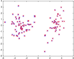
  Figure 19: An example illustrating the conjecture of this section. Given all statements of the kind ($\star$ ‣ 1) for the set of blue points, an algorithm for ordinal embedding is able to almost perfectly recover the point configuration up to a similarity transformation (red points—after a Procrustes analysis).

  This raises the question whether density estimation or solving any other local problem is possible at all given only ordinal distance information of the kind ($\star$ ‣ 1), and indeed the answer is negative for intrinsically one-dimensional data sets: Consider data points $x_{1},\ldots,x_{n}$ on the real line and assume $d$ to be the Euclidean metric. Then the ordinal distance information given by all statements of the kind ($\star$ ‣ 1) only depends on the order of the data points: given any three data points, the center is always given by the data point sitting in the middle, and any order-preserving transformation of the data points will give rise to exactly the same ordinal distance information. For this reason it is impossible to estimate any local property of an underlying distribution, and ordinal distance information of the kind ($\star$ ‣ 1) comes along with a substantial loss in effective information compared to similarity triplets, that is answers to (18): while, under some assumptions on the data points, all similarity triplets asymptotically uniquely determine the actual positions of the points on the real line up to a similarity transformation (Proposition 10 in Kleindessner and von Luxburg, 2014), all statements of the kind ($\star$ ‣ 1) only determine the ranking of the data points up to inversion. However, such a loss in information does not seem to occur when dealing with data sets of higher intrinsic dimensionality: If we start with data points from $\mathbb{R}^{m}$ for $m\geq 2$ (again equipped with the Euclidean metric) that are reasonably scattered, collect all statements of the kind ($\star$ ‣ 1), and provide them as input to an ordinal embedding algorithm, then the algorithm is able to almost perfectly recover the configuration of the data points up to a similarity transformation. An example of this happening can be seen in Figure 19 for a set of 100 points in $\mathbb{R}^{2}$: the blue points are the data points that we start with and the red ones are the recovered data points after a Procrustes analysis, that is aligning the points of the ordinal embedding with the original ones via a similarity transformation. We have observed this phenomenon for a broad variety of point configurations in Euclidean spaces $\mathbb{R}^{m}$ of arbitrary dimensions $m\geq 2$ and want to state it as a conjecture. We formulate the conjecture similarly to the theorems in Kleindessner and von Luxburg (2014) and Arias-Castro (2015), which state the asymptotic uniqueness property for ordinal data consisting of answers to general dissimilarity comparisons (17) and for similarity triplets, that is answers to comparisons (18).

  Conjecture: Let $B_{1}$ and $B_{2}$ be two closed and bounded balls in $\mathbb{R}^{m}$, $m\geq 2$, with arbitrary centers and radii. Let $(x_{n})_{n\in\mathbb{N}}$ be a sequence of points $x_{n}\in B_{1}$ such that $\{x_{n}:n\in\mathbb{N}\}$ is dense in $B_{1}$. For $n\in\mathbb{N}$, let $X_{n}=\{x_{1},\ldots,x_{n}\}$ and let $Y_{n}=\{y_{1}^{n},\ldots,y_{n}^{n}\}\subseteq B_{2}$ be an ordinal embedding of $X_{n}$ that preserves all statements of the kind ($\star$ ‣ 1) (but not necessarily any other ordinal relationships). Then there exists a sequence $(S_{n})_{n\in\mathbb{N}}$ of similarity transformations $S_{n}:\mathbb{R}^{m}\rightarrow\mathbb{R}^{m}$ such that

  $$\max_{i=1,\ldots,n}\left\|S_{n}(y_{i}^{n})-x_{i}\right\|\rightarrow 0~{}~{}~{}\text{as}~{}~{}n\rightarrow 0.$$

  Hence, there is hope: if our conjecture holds, when dealing with a Euclidean data set of known intrinsic dimension, which is greater than one, then all statements of the kind ($\star$ ‣ 1) asymptotically contain all cardinal distance information up to rescaling. At least for such a data set we may hope that, in principle, we are able to solve any local problem that we can solve in a standard machine learning setting of cardinal distance information also in a setting of ordinal distance information of the type ($\star$ ‣ 1). However, it remains an open problem how to solve a local problem in practice except for an embedding approach.
  

• Active learning: Algorithms 1 to 5 can deal with arbitrary collections of statements of the kind ($\star$ ‣ 1) that are gathered before the application of the algorithm and are provided as input all at once. However, in many scenarios one might have the chance to actively query statements for intentionally chosen triples of objects. In such a scenario an algorithm for a machine learning task should interact with the process of querying statements and adaptively choose triples of objects for which statements are to be queried in such a way that the task at hand is solved as fast, accurately, cheaply, … as possible. For the problems of medoid estimation or outlier identification it is easy to adapt Algorithm 1 and Algorithm 2 in order to derive adaptive versions: starting with rough estimates of values $LD(O)$ for every object $O$ in the data set, one could immediately rule out some objects with very small (or high) estimated values and continue improving only estimates of the values of the remaining objects by querying further statements only for them. This strategy has been suggested by Heikinheimo and Ukkonen (2013) for their method for medoid estimation. Studying the questions whether such a strategy comes with any guarantees, whether there might be better alternatives (of course, this depends on what one wants to achieve), or whether similar approaches apply to Algorithms 3 to 5 is left for future work.

Two further follow-up questions are: I. If one is free to choose the particular type of ordinal data that one is working with, for example in a crowdsourcing scenario, then which type is most appropriate for which problems (in terms that it is both informative for the problem at hand and can easily be provided by the crowd)? II. How can we fix the error in the proof of Theorem 6 in Liu and Modarres (2011) (see Section 5.2)?

Acknowledgments

This work was supported by the Institutional Strategy of the University of Tübingen (Deutsche Forschungsgemeinschaft, ZUK 63).

References

- Agarwal et al. (2007) S. Agarwal, J. Wills, L. Cayton, G. Lanckriet, D. Kriegman, and S. Belongie. Generalized non-metric multidimensional scaling. In International Conference on Artificial Intelligence and Statistics (AISTATS), 2007.
- Agostinelli and Romanazzi (2008) C. Agostinelli and M. Romanazzi. Local depth of multivariate data. Technical report, Ca’ Foscari University of Venice, 2008.
- Agostinelli and Romanazzi (2011) C. Agostinelli and M. Romanazzi. Local depth. Journal of Statistical Planning and Inference, 141(2):817–830, 2011.
- Amid and Ukkonen (2015) E. Amid and A. Ukkonen. Multiview triplet embedding: Learning attributes in multiple maps. In International Conference on Machine Learning (ICML), 2015.
- Amid et al. (2016) E. Amid, N. Vlassis, and M. Warmuth. -exponential triplet embedding. arXiv:1611.09957 [cs.AI], 2016.
- Andrade and de Figueiredo (2001) D. V. Andrade and L. H. de Figueiredo. Good approximations for the relative neighbourhood graph. In Canadian Conference on Computational Geometry (CCCG), 2001.
- Arias-Castro (2015) E. Arias-Castro. Some theory for ordinal embedding. arXiv:1501.02861 [math.ST], 2015.
- Bai et al. (2000) Z. Bai, J. Demmel, J. Dongarra, A. Ruhe, and H. van der Vorst, editors. Templates for the Solution of Algebraic Eigenvalue Problems: A Practical Guide. Society for Industrial and Applied Mathematics, 2000.
- Barnett and Lewis (1978) V. Barnett and T. Lewis. Outliers in Statistical Data. Wiley, 1978.
- Bartoszynski et al. (1997) R. Bartoszynski, D. K. Pearl, and J. Lawrence. A multidimensional goodness-of-fit test based on interpoint distances. Journal of the American Statistical Association, 92(438):577–586, 1997.
- Blum et al. (1973) M. Blum, R. W. Floyd, V. Pratt, R. L. Rivest, and R. E. Tarjan. Time bounds for selection. Journal of Computer and System Sciences, 7:448–461, 1973.
- Borg and Groenen (2005) I. Borg and P. Groenen. Modern Multidimensional Scaling: Theory and Applications. Springer, 2005.
- Bose et al. (2012) P. Bose, V. Dujmović, F. Hurtado, J. Iacono, S. Langerman, H. Meijer, V. Sacristán, M. Saumell, and D. R. Wood. Proximity graphs: , , , and . International Journal of Computational Geometry and Applications, 22(5):439–469, 2012.
- Botelho et al. (2007) F. C. Botelho, R. Pagh, and N. Ziviani. Simple and space-efficient minimal perfect hash functions. In Workshop on Algorithms and Data Structures (WADS), 2007.
- Cascos (2009) I. Cascos. Data depth: Multivariate statistics and geometry. In W. S. Kendall and I. Molchanov, editors, New Perspectives in Stochastic Geometry. Oxford University Press, 2009.
- Chang et al. (1992) M. S. Chang, C. Y. Tang, and R. C. T. Lee. Solving the euclidean bottleneck matching problem by -relative neighborhood graphs. Algorithmica, 8(1–6):177–194, 1992.
- Chen et al. (2009) Y. Chen, X. Dang, H. Peng, and H. L. Bart, Jr. Outlier detection with the kernelized spatial depth function. IEEE Transactions on Pattern Analysis and Machine Intelligence, 31(2):288–305, 2009.
- Correa and Lindstrom (2012) C. D. Correa and P. Lindstrom. Locally-scaled spectral clustering using empty region graphs. In ACM International Conference on Knowledge Discovery and Data Mining (SIGKDD), 2012.
- Cristianini and Shawe-Taylor (2000) N. Cristianini and J. Shawe-Taylor. An Introduction to Support Vector Machines and other Kernel-Based Learning Methods. Cambridge University Press, 2000.
- Dang and Serfling (2010) X. Dang and R. Serfling. Nonparametric depth-based multivariate outlier identifiers, and masking robustness properties. Journal of Statistical Planning and Inference, 140(1):198–213, 2010.
- Elmore et al. (2006) R. T. Elmore, T. P. Hettmansperger, and F. Xuan. Spherical data depth and a multivariate median. In R. Y. Liu, R. Serfling, and D. L. Souvaine, editors, Data Depth: Robust Multivariate Analysis, Computational Geometry and Applications. American Mathematical Society, 2006.
- Freeman (1978) L. C. Freeman. Centrality in social networks: Conceptual clarification. Social Networks, 1(3):215–239, 1978.
- Gabriel and Sokal (1969) K. R. Gabriel and R. R. Sokal. A new statistical approach to geographic variation analysis. Systematic Zoology, 18(3):259–278, 1969.
- Ghosh and Chaudhuri (2005) A. K. Ghosh and P. Chaudhuri. On maximum depth and related classifiers. Scandinavian Journal of Statistics, 32(2):327–350, 2005.
- Hagerup and Tholey (2001) T. Hagerup and T. Tholey. Efficient minimal perfect hashing in nearly minimal space. In Symposium on Theoretical Aspects of Computer Science (STACS), 2001.
- Haghiri et al. (2017) S. Haghiri, D. Ghoshdastidar, and U. von Luxburg. Comparison based nearest neighbor search. In International Conference on Artificial Intelligence and Statistics (AISTATS), 2017.
- Hashimoto et al. (2015) T. B. Hashimoto, Y. Sun, and T. S. Jaakkola. Metric recovery from directed unweighted graphs. In International Conference on Artificial Intelligence and Statistics (AISTATS), 2015.
- Heikinheimo and Ukkonen (2013) H. Heikinheimo and A. Ukkonen. The crowd-median algorithm. In Conference on Human Computation and Crowdsourcing (HCOMP), 2013.
- Heim et al. (2015) E. Heim, M. Berger, L. M. Seversky, and M. Hauskrecht. Efficient online relative comparison kernel learning. In SIAM International Conference on Data Mining (SDM), 2015.
- Jain et al. (2016) L. Jain, K. G. Jamieson, and R. Nowak. Finite sample prediction and recovery bounds for ordinal embedding. In Neural Information Processing Systems (NIPS), 2016.
- Jamieson and Nowak (2011) K. G. Jamieson and R. Nowak. Low-dimensional embedding using adaptively selected ordinal data. In Conference on Communication, Control, and Computing, 2011.
- Jaromczyk and Toussaint (1992) J. W. Jaromczyk and G. T. Toussaint. Relative neighborhood graphs and their relatives. Proceedings of the IEEE, 80(9):1502–1517, 1992.
- Kleindessner and von Luxburg (2014) M. Kleindessner and U. von Luxburg. Uniqueness of ordinal embedding. In Conference on Learning Theory (COLT), 2014.
- Kleindessner and von Luxburg (2015) M. Kleindessner and U. von Luxburg. Dimensionality estimation without distances. In International Conference on Artificial Intelligence and Statistics (AISTATS), 2015.
- Kruskal (1964a) J. B. Kruskal. Multidimensional scaling by optimizing goodness of fit to a nonmetric hypothesis. Psychometrika, 29(1):1–27, 1964a.
- Kruskal (1964b) J. B. Kruskal. Nonmetric multidimensional scaling: A numerical method. Psychometrika, 29(2):115–129, 1964b.
- Lawrence (1996) J. Lawrence. Interpoint Distance Methods for the Analysis of High Dimensional Data. PhD thesis, The Ohio State University, 1996.
- Leskovec et al. (2007) J. Leskovec, J. Kleinberg, and C. Faloutsos. Graph evolution: Densification and shrinking diameters. ACM Transactions on Knowledge Discovery from Data, 1(1), 2007. Data available on https://snap.stanford.edu/data/.
- Li et al. (2012) J. Li, J. A. Cuesta-Albertos, and R. Y. Liu. DD-classifier: Nonparametric classification procedure based on DD-plot. Journal of the American Statistical Association, 107(498):737–753, 2012.
- Li et al. (2011) M. Li, X.-C. Lian, J. T.-Y. Kwok, and B.-L. Lu. Time and space efficient spectral clustering via column sampling. In IEEE Conference on Computer Vision and Pattern Recognition (CVPR), 2011.
- Liu et al. (2004) C. Liu, K. Wu, and T. He. Sensor localization with ring overlapping based on comparison of received signal strength indicator. In IEEE International Conference on Mobile Ad-hoc and Sensor Systems (MASS), 2004.
- Liu (1988) R. Y. Liu. On a notion of simplicial depth. Proceedings of the National Academy of Sciences of the United States of America, 85(6):1732–1734, 1988.
- Liu (1990) R. Y. Liu. On a notion of data depth based on random simplices. The Annals of Statistics, 18(1):405–414, 1990.
- Liu (1992) R. Y. Liu. Data depth and multivariate rank tests. In Y. Dodge, editor, L1-Statistical Analysis and Related Methods. North Holland, 1992.
- Liu et al. (1999) R. Y. Liu, J. M. Parelius, and K. Singh. Multivariate analysis by data depth: descriptive statistics, graphics and inference. The Annals of Statistics, 27(3):783–840, 1999.
- Liu and Modarres (2011) Z. Liu and R. Modarres. Lens data depth and median. Journal of Nonparametric Statistics, 23(4):1063–1074, 2011.
- Manning et al. (2008) C. D. Manning, P. Raghavan, and H. Schütze. Introduction to Information Retrieval. Cambridge University Press, 2008.
- Mosler (2013) K. Mosler. Depth statistics. In C. Becker, R. Fried, and S. Kuhnt, editors, Robustness and Complex Data Structures: Festschrift in Honour of Ursula Gather. Springer, 2013.
- Sánchez et al. (1997a) J. S. Sánchez, F. Pla, and F. J. Ferri. On the use of neighbourhood-based non-parametric classifiers. Pattern Recognition Letters, 18(11–13):1179–1186, 1997a.
- Sánchez et al. (1997b) J. S. Sánchez, F. Pla, and F. J. Ferri. Prototype selection for the nearest neighbour rule through proximity graphs. Pattern Recognition Letters, 18(6):507–513, 1997b.
- Schultz and Joachims (2003) M. Schultz and T. Joachims. Learning a distance metric from relative comparisons. In Neural Information Processing Systems (NIPS), 2003.
- Serfling (2006) R. Serfling. Depth functions in nonparametric multivariate inference. In R. Y. Liu, R. Serfling, and D. L. Souvaine, editors, Data Depth: Robust Multivariate Analysis, Computational Geometry and Applications. American Mathematical Society, 2006.
- Shalev-Shwartz and Ben-David (2014) S. Shalev-Shwartz and S. Ben-David. Understanding Machine Learning: From Theory to Algorithms. Cambridge University Press, 2014.
- Shaw and Jebara (2009) B. Shaw and T. Jebara. Structure preserving embedding. In International Conference on Machine Learning (ICML), 2009.
- Shepard (1962a) R. N. Shepard. The analysis of proximities: Multidimensional scaling with an unknown distance function. I. Psychometrika, 27(2):125–140, 1962a.
- Shepard (1962b) R. N. Shepard. The analysis of proximities: Multidimensional scaling with an unknown distance function. II. Psychometrika, 27(3):219–246, 1962b.
- Shi and Malik (2000) J. Shi and J. Malik. Normalized cuts and image segmentation. IEEE Transactions on Pattern Analysis and Machine Intelligence, 22(8):888–905, 2000.
- Stewart et al. (2005) N. Stewart, G. D. A. Brown, and N. Chater. Absolute identification by relative judgment. Psychological Review, 112(4):881–911, 2005.
- Tamuz et al. (2011) O. Tamuz, C. Liu, S. Belongie, O. Shamir, and A. T. Kalai. Adaptively learning the crowd kernel. In International Conference on Machine Learning (ICML), 2011.
- Terada and von Luxburg (2014) Y. Terada and U. von Luxburg. Local ordinal embedding. In International Conference on Machine Learning (ICML), 2014. Code available on https://cran.r-project.org/web/packages/loe.
- Toussaint (1980) G. T. Toussaint. The relative neighbourhood graph of a finite planar set. Pattern Recognition, 12(4):261–268, 1980.
- Toussaint (2014) G. T. Toussaint. Applications of the relative neighbourhood graph. In International Conference on Advances in Computing, Communication and Information Technology (CCIT), 2014.
- Toussaint and Berzan (2012) G. T. Toussaint and C. Berzan. Proximity-graph instance-based learning, support vector machines, and high dimensionality: An empirical comparison. In International Conference on Machine Learning and Data Mining (MLDM), 2012.
- Toussaint et al. (1984) G. T. Toussaint, B. K. Bhattacharya, and R. S. Poulsen. The application of voronoi diagrams to non-parametric decision rules. In Symposium on the Interface of Computing Science and Statistics, 1984.
- Tukey (1974) J. W. Tukey. Mathematics and the picturing of data. In International Congress of Mathematicians (ICM), 1974.
- Ukkonen et al. (2015) A. Ukkonen, B. Derakhshan, and H. Heikinheimo. Crowdsourced nonparametric density estimation using relative distances. In Conference on Human Computation and Crowdsourcing (HCOMP), 2015.
- Van Bever (2013) G. Van Bever. Contributions to Nonparametric and Semiparametric Inference based on Statistical Depth. PhD thesis, Université libre de Bruxelles, 2013.
- van der Maaten and Weinberger (2012) L. J. P. van der Maaten and K. Q. Weinberger. Stochastic triplet embedding. In IEEE International Workshop on Machine Learning for Signal Processing (MLSP), 2012. Code available on http://homepage.tudelft.nl/19j49/ste.
- von Luxburg (2007) U. von Luxburg. A tutorial on spectral clustering. Statistics and Computing, 17(4):395–416, 2007.
- von Luxburg and Alamgir (2013) U. von Luxburg and M. Alamgir. Density estimation from unweighted k-nearest neighbor graphs: a roadmap. In Neural Information Processing Systems (NIPS), 2013.
- Wilber et al. (2014) M. J. Wilber, I. S. Kwak, and S. J. Belongie. Cost-effective hits for relative similarity comparisons. In Conference on Human Computation and Crowdsourcing (HCOMP), 2014.
- Xiao et al. (2006) L. Xiao, R. Li, and J. Luo. Sensor localization based on nonmetric multidimensional scaling. In International Conference on Sensing, Computing and Automation (ICSCA), 2006.
- Yan et al. (2009) D. Yan, L. Huang, and M. I. Jordan. Fast approximate spectral clustering. In ACM International Conference on Knowledge Discovery and Data Mining (SIGKDD), 2009.
- Yang (2014) M. Yang. Depth Functions, Multidimensional Medians and Tests of Uniformity on Proximity Graphs. PhD thesis, The George Washington University, 2014.
- Zuo and Serfling (2000) Y. Zuo and R. Serfling. General notions of statistical depth function. The Annals of Statistics, 28(2):461–482, 2000.